SC-CAN: Spectral Convolution and Channel Attention Network for Wheat Stress Classification

Abstract

Biotic and abiotic plant stress (e.g., frost, fungi, diseases) can significantly impact crop production. It is thus essential to detect such stress at an early stage before visual symptoms and damage become apparent. To this end, this paper proposes a novel deep learning method, called Spectral Convolution and Channel Attention Network (SC-CAN), which exploits the difference in spectral responses of healthy and stressed crops. The proposed SC-CAN method comprises two main modules: (i) a spectral convolution module, which consists of dilated causal convolutional layers stacked in a residual manner to capture the spectral features; (ii) a channel attention module, which consists of a global pooling layer and fully connected layers that compute inter-relationship between feature map channels before scaling them based on their importance level (attention score). Unlike standard convolution, which focuses on learning local features, the dilated convolution layers can learn both local and global features. These layers also have long receptive fields, making them suitable for capturing long dependency patterns in hyperspectral data. However, because not all feature maps produced by the dilated convolutional layers are important, we propose a channel attention module that weights the feature maps according to their importance level. We used SC-CAN to classify salt stress (i.e., abiotic stress) on four datasets (Chinese Spring (CS), Aegilops columnaris (co(CS)), Ae. speltoides auchery (sp(CS)), and Kharchia datasets) and Fusarium head blight disease (i.e., biotic stress) on Fusarium dataset. Reported experimental results show that the proposed method outperforms existing state-of-the-art techniques with an overall accuracy of 83.08%, 88.90%, 82.44%, 82.10%, and 82.78% on CS, co(CS), sp(CS), Kharchia, and Fusarium datasets, respectively.

1. Introduction

Stress in wheat crops can be caused by abiotic factors (e.g., salt, drought, or extreme temperatures) or biotic factors (e.g., pathogens and insects) [1]. Such stress affects wheat growth and productivity [2] and can be identified by observing visual symptoms [3]. A study in [4] successfully detected stress by analyzing the visual symptoms using an image processing technique. However, by the time visual symptoms appear, it is often too late to put in place appropriate crop management solutions to mitigate crop losses. Early manifestation of plant stress responses include changes in chlorophyll content, as well as cellular metabolism and tissue degradation [5]. These changes affect in turn the plant’s spectral reflectance, which can be captured by hyperspectral sensors. Hence, spectral information (reflection intensity per waveband in hyperspectral data) can be leveraged for the early detection of crop stress.

Spectral information is typically captured at hundreds of narrow bands, where adjacent bands tend to be highly correlated, resulting in considerable redundancy [6,7]. Analyzing spectral information is challenging because of its high dimensionality and redundancy [8]. A number of methods have been proposed to analyze spectral data for wheat-stress classification, e.g., Bayesian [9], random forest, and Support Vector Machine (SVM) [10]. However, these methods rely heavily on handcrafted features, which are usually designed for a specific task. They also cannot be generalized, limiting their applicability [11]. In contrast, recent deep learning techniques can learn features automatically from the data [11,12], making them a promising alternative for spectral data analysis.

A number of these deep learning studies treat spectral data as a sequence. A deep learning method commonly used for sequential data are Recurrent Neural Networks (RNNs) [13,14]. Mou et al. [15] used RNNs to extract features from the spectral data. However, RNNs are prone to gradient vanishing or exploding problems if the sequence is long [16,17]. As a result, RNNs are less suitable for long data sequences. To address this issue, Lipton et al. [18] proposed Long Short-Term Memory (LSTM), which replaced the recurrent hidden nodes with memory cells, so that the gradient can go across several time steps without vanishing or exploding. LSTM network was used to extract features from the spectral data [16,19]. However, LSTM has a limited attention span, and cannot capture long dependency patterns [20], which may exist in the hyperspectral data. Moreover, since LSTM and RNNs have recurrent connections, their training process is time-consuming for a very long sequence.

Other studies proposed convolutional neural network (CNN) to extract features from spectral data. The convolutional networks do not have recurrent connections, so they are faster to train than LSTM or RNNs. Since the spectral data structure is a one-dimensional (1D) array, Hu et al. [21] proposed to use CNN with 1D kernels to extract these spectral features. If the 1D-CNN network is shallow, it will only be able to extract local features as its kernels only have a short receptive field [22]. Stacking more layers is thus required to increase the receptive field. This process will increase the number of parameters and lead to over-fitting problems. In order to overcome this problem, Jin et al. [23] proposed to convert spectral data into 2D array and use 2D convolution kernels to help extract global spectral features. The proposed network achieved a better performance than its 1D-CNN counterpart. However, the 2D kernels may lose certain local features when implemented on the reshaped spectral data.

In order to overcome the aforementioned shortcomings, we propose spectral convolution modules that consist of dilated convolutional layers with 1D filters to extract spectral features. The use of dilated convolutional layers is inspired by WaveNet [24], which was originally developed for speech generation, but with two important differences. First, our dilated convolutional layers use acausal dilated convolution to learn the relationship between adjacent bands in contrast to causal dilated convolution in WaveNet, which only learns from previous states. Second, our dilated convolutional layers use recurrent connections to minimize the exploding or vanishing gradient problem, and to minimize information continuity loss [25,26]. Our proposed spectral convolution module is able to extract both local and global features from the long spectral data for the following reasons. The first dilated convolution layer has a dilation rate of 1, which corresponds to a standard convolution, allowing it to extract the local features. By increasing the dilation rate, the receptive field for the dilated convolutional layer gradually becomes larger. Consequently, the dilated convolution layers are able to extract various levels of global features.

Every dilated convolutional layer employs C filters to produce C channel-wise feature maps. Each filter works as a detector; thus, a channel-wise feature map is actually the detector response map of the corresponding filter [27]. However, certain feature maps may contain very insignificant information, which will have little effect on the overall network performance. As a result, if all feature maps are treated equally without taking importance into account, the network performance may be adversely affected. The work of [28] handles this issue by removing the uninformative feature maps and their corresponding filters in the current layer and in kernels of the next layer.

Despite containing little information, the less important feature maps may still be useful. Discarding them completely like in [28] may deteriorate the network performance. Hence, in this paper, we proposed to add a channel attention module after every dilated convolutional layer to learn the importance level of each feature map channel and to scale each feature map channel based on its importance level (attention score). Here, the informative feature maps will be multiplied with a large attention score, and the uninformative feature maps will be multiplied with a small attention score. Hence, each feature map is treated differently based on its importance level.

We then apply our proposed network to the problem of stress classification in wheat crops, and we analyse two types of wheat stress. The first is wheat crop stress caused by Fusarium infection (i.e., biotic stress) using the Fusarium head blight (FHB) disease dataset, used in [23]. Fusarium infection can harm the physiological functions of wheat, resulting in wheat yield reduction and grain quality deterioration [29]. Additionally, several fungal toxins, including the poisonous one Deoxynivalenol (DON), will be produced after the wheat is infected, making the FHB infected grain unsafe for food [30]. Detecting the disease earlier can reduce the loss caused by the FHB disease.

The second type of stress that we analysed is caused by excess salt (i.e., abiotic stress). Salt stress causes hyperosmotic stress and ion imbalance that affect the growth and yields of crop plants [31]. A study in soybean plants [31] showed that a high concentration of NaCl affects the plant reflectance in the range of 600–730 nm. Although a study in melon plants [32] found that NDVI_750-705 (Normalized Different Vegetation Index based on 705 and 750 nm) and Water Index based on 900 and 970 nm have a significant relationship with salt stress. Those studies showed that different plants might have different spectral regions that significantly relate to salt stress. Finding the spectral regions manually when working with a new plant type is ineffective. Hence, instead of manually selecting the important spectral regions, the study in [10] presented an ensemble feature selection method to select several most important bands from 215 bands acquired by a spectral sensor. Further study in sugarcane plant by [33] that compares all bands, five principal components from PCA, and nine vegetation indexes as the feature input of SVM showed that SVM that used all of the band as input is superior. Using all of the bands and processing them with a robust machine learning technique is a promising approach for salt stress classification. Hence, in this study, we proposed a deep learning technique, to classify salt stress in wheat. We used four salt stress datasets: Chinese Spring (CS), Aegilops columnaris (co(CS)), Ae.speltoides auchery (sp(CS)), and Kharchia datasets. Only CS dataset was reported in the study by [10]. Reported experimental results show that our proposed network, dubbed SC-CAN (Spectral Convolution and Channel Attention Network), performs better than the state-of-the-art methods.

In summary, our contributions in this paper are three-fold: (1) We leverage causal dilated convolutional layers in the spectral convolution modules to capture both local and global spectral features. In contrast, a shallow network with standard convolution can only extract local features. (2) By introducing a channel attention module, we make our network pay more attention to informative feature maps. Our experiments show that the channel attention module improves the network’s performance and stability. (3) We achieve state-of-the-art performance for the classification of salt and Fusarium stress. Our proposed method achieves an F1-mean of 83.03% on the CS dataset compared to SFS_Forward with F1-mean of 77.71%. For the Fusarium dataset, we obtain an overall accuracy (OA) of 82.78% compared to 74.30% for the 2D-CNN-BidGRU. These findings demonstrate that the proposed SC-CAN network can detect the stress in wheat even before the visual symptoms arise. Section 2 provides an overview of the related works, including dilated convolution and attention modules. Section 3 explains the proposed SC-CAN method. Experimental results and performance evaluation are discussed in Section 4. The research findings are concluded in Section 5.

2. Related Works

2.1. Dilated Convolution

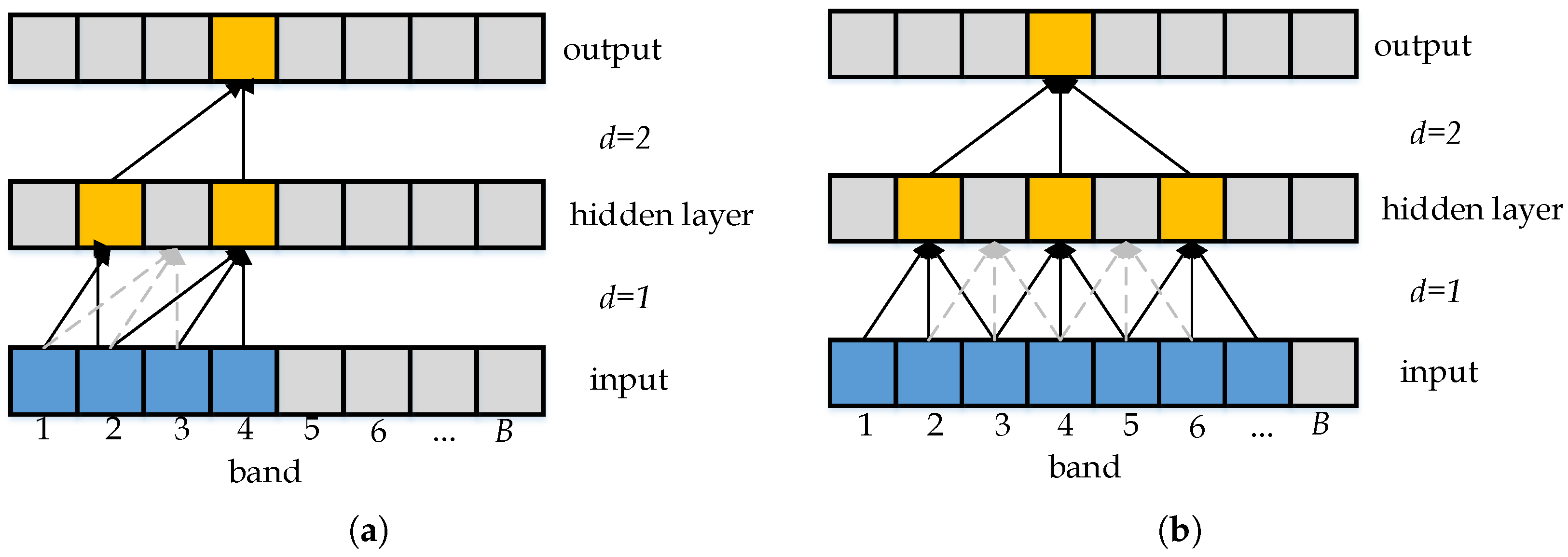
In dilated convolutions, the kernel is applied to an area longer than its length by inserting $d-1$ zeros between kernel elements, where d is the dilation rate whose value is a positive integer [24]. The value of d varies. The larger the d, the larger the receptive field. When d is 1, the dilated convolution will be the same as the standard convolution (see Figure 1a). Another example of a frequently used dilation rate is $2^{i-1}$ (see Figure 1b), where i is the layer number. A network with a dilated convolution has a wider receptive field than a network with a standard convolution, as shown in Figure 1b.

Figure 1a,b show that the deepest feature map is in the output layer. Since the receptive field size of each pixel in the output feature map is much smaller than the size of the input signal (Figure 1a), each pixel contains local features. As an example, the value of a feature in the middle of the map, represented in orange, depends only on the input in bands 5–11. Changes in the input value in band one will not affect the feature value in the orange pixel. There is empirical evidence that pixels located “far away” from their corresponding feature do not affect the value of that feature. Since these features only depend on pixels whose position is local to them, they are called “local” features. Unlike standard convolutions, dilated convolutions (Figure 1b) can extract global features even when the network is shallow. From the figure, the feature value of the orange pixel in the output feature map is based on the input values from band one through band B; therefore, these features are called “global”. In the event that one of the values in the input bands changes, the value in the orange pixel will also change. Therefore, dilated convolution can capture long-range dependencies.

Dilated convolutions can be used with 1D, 2D, or 3D kernels. Studies have used dilated convolutions with 2D kernels to extract spatial features from hyperspectral images [34,35,36,37]. These studies differ in terms of network structure and dilation rate. The study in [34] used a constant dilation rate of 3, while [35,36] used gradually increasing dilation rates, and the study in [37] used gradually increased dilation rates followed by convolutional layers with gradually decreased dilation rates. Overall, these studies showed that dilated convolution: (1) can reduce spatial information loss [35], (2) can learn discriminative spatial features and expand the receptive field of the convolution kernel without increasing computational complexity [34,37], and, thus, (3) efficient for classification [36].

The benefit of dilated convolution for the extraction of spatial features encourages us to use it for the extraction of spectral features as well. It is important to extract spectral features from data in several situations, e.g., when the data contain only spectral information (data acquired from non-imaging sensors) or when we wish to explore vegetation interaction with spectral reflectance [38]. Due to the fact that spectral signal data are one-dimensional, dilated convolution with 2D kernels cannot be applied.

The hyperspectral data that only contains spectral information are structurally adapted to convolution with 1D kernel. A dilated convolution with 1D kernel was first proposed in WaveNet for speech generation [24]. Given a sequence of input text, WaveNet can predict a sequence of T output speech, where T is the length of the output data. The convolution process in WaveNet is causal to ensure that the prediction generated at time t is independent of any future steps, where $t\in T$. Unlike the speech generation problem, our problem is a classification problem, which means that the predictions generated by our model can be affected by all the spectral data. For that reason, the convolution process used in this paper is acausal, as detailed in Section 3.1.

2.2. Attention Module

An attention module can help a network focus on informative features [39,40]. An attention module can also describe the global dependencies between input and output [41]. One of the attention mechanisms is self-attention, which allows an input in the input sequence to interact with other inputs in the sequence and learn which inputs the module should pay more attention to. This technique is popular in many fields, such as abstractive summarization, textual entitlement, and reading comprehension [41,42,43,44].

In image processing, a spatial attention module was used in [40] to encode the spatial area where the network attends most to make output decisions. In HSI, attention mechanisms have been used in several studies. Mou et al. [45] designed a spectral attention module at the beginning of their network using a gating mechanism. In contrast to [45], Liu et al. [46] applied the attention process to a group of spectral data. In both [45,46], the spectral attention modules improved the network performance. At the same time, Lorenzo et al. [47] coupled attention-based convolution with an anomaly detection technique for hyperspectral band selection. Their experiments showed that the combination between the attention module and the anomaly detection could be used for band selection, although it did not improve the classification performance. The aforementioned works are similar in that an attention module is used to help the networks focus on important spectral information.

In convolution-based feature extraction, each filter works as a detector, whose output is saved onto a channel-wise feature map. Each feature map may contain a different amount of information. Certain feature maps may contain rich knowledge that is important to the network, while others do not. Hence, in contrast to [45,46,47] which use spectral attention, our self-attention mechanism focuses on channel attention to make the model pay more attention to informative feature maps.

To implement a self-attention mechanism, several studies used convolutional layers to compute attention between an input and its neighbours (local attention). This self-attention type is suitable for inputs that have neighbourhood relationships, such as spatial relationships between pixels in an image. Hence, convolutional-based self-attention is widely used for computing spatial attention [25,48,49], and spectral attention [47]. However, this type of self-attention may not suit channel attention because feature map channels do not have neighbourhood relationships. Feature map channels may have global relationships. Scaled dot product attention can be used to compute the global attention of inputs. This attention computes the relationship between a query and a set of key-values [41], where for self-attention, the query and key-values are from the same inputs that have been projected by different projections layers. This kind of attention has been widely used for encoder–decoder attention in machine-translation problems. However, its impact on self-attention is not significant [50]. Another technique that can be used to compute global relationships between inputs is a fully connected layer. This technique has successfully been used to compute spectral self-attention [46]. In this paper, we exploit fully connected layers to compute the global relationship between feature map channels. In contrast to the spectral self-attention [46] which squeezes a group of bands, in this paper, we squeeze each feature map channel, as detailed in Section 3.2.

3. Proposed Methodology

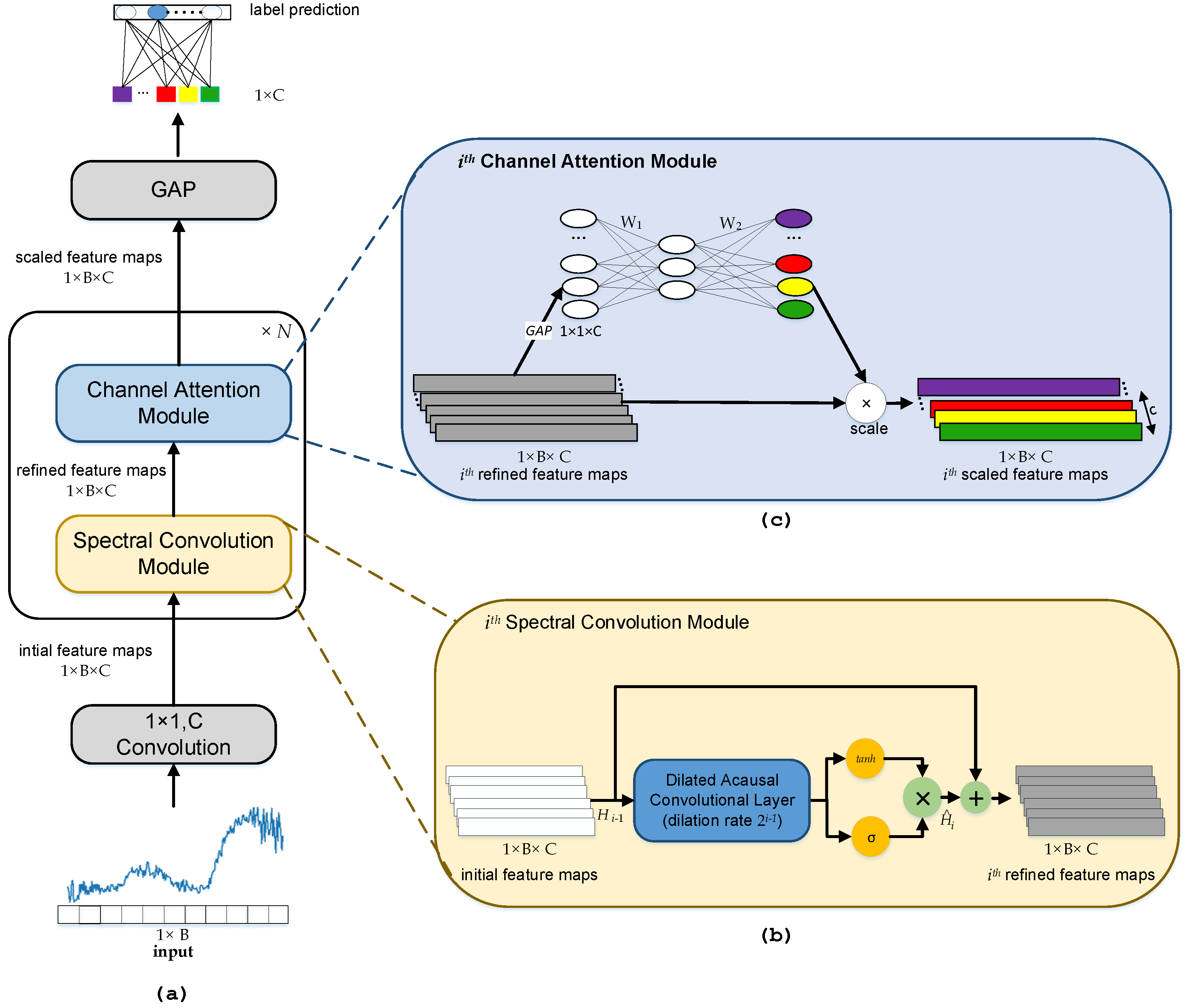
The SC-CAN network basic diagram is shown in Figure 2a, with details of the spectral convolution and channel attention modules provided in Figure 2b,c. The network’s input is a spectral signal, which can be considered as a vector of size $1\times B$, where B is the number of bands. We consider the input as a sequence of spectral bands.

In the training phase, each input is first convolved by a 1D convolution layer with C output channels and kernels of size $1\times 1$ to project the input into C channel-wise feature maps (initial feature maps). So, the initial feature maps size is $1\times B\times C$, where C is the number of output channels, i.e., 196. We need projection because we used residual connections in every dilated convolutional layer, and the output channel of these convolution layers is C, so to make a residual connection, we have to make sure the dimension of feature maps before convolution and after convolution is the same. The intermediate feature maps are then processed by N dilated convolutional layers and channel attention module consecutively. Their deepest output is Nth scaled feature maps.

The Nth scaled feature maps with the highest level features that have been scaled by the channel attention module have a size of $1\times B\times C$. In addition, to obtain the global information about each feature map’s channel for classification, the scaled feature maps are processed by global average pooling (GAP). With this process, the scaled feature maps will be resized from $1\times B\times C$ to $1\times C$. Then, a Dropout layer with a 0.1 rate is used as a regularizer to minimize the over-fitting problem, and a fully-connected layer with a softmax activation function is used to predict labels. To calculate the training loss, the label prediction is compared with the true label. In addition, the training loss is used to update the SC-CAN training parameters. In order to build a trained SC-CAN model, these processes must be repeated several times (epochs).

Test data prediction labels are generated based on the classification of the test inputs by the trained SC-CAN model during testing. A comparison is made between the predictions and the true labels in order to calculate the performance masures.

3.1. Spectral Convolution Module

A dilated convolutional layer is incorporated into each of our N spectral convolution modules. Hence, we can consider the dilated convolutional layer at the ith spectral convolution module as the ith dilated convolutional layer. The dilation factor of the dilated convolutional layer is $2^{i-1}$, where i is the index of the spectral convolution module, $i=\{1,2,...,N\}$. The dilation factor that increases exponentially with depth results in the exponential growth of the receptive field, and thus each dilated convolutional layer can extract a different level of features.

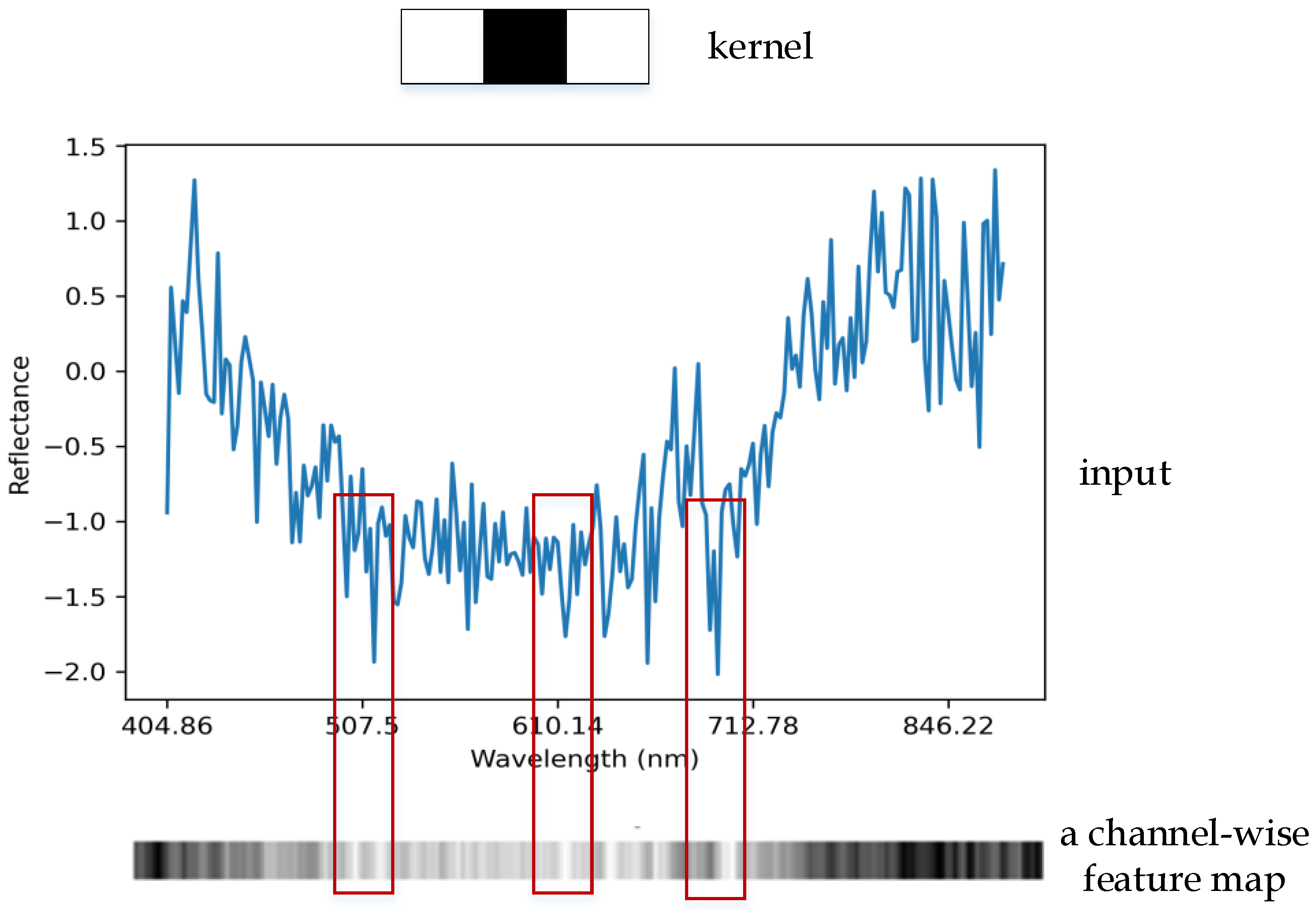
The first dilated convolutional layer ($i=1$) has a dilation factor of 1, $d=2^{i-1}=2^{1-1}=2^0=1$. As a special case, dilated convolution with dilation factor of 1 is the same with standard convolution that can extract local features. The actual example and result of the standard convolution process for spectral information in producing local features are shown in Figure 3. Given a kernel (Figure 3 (top)) and spectral input (Figure 3 (middle)), the result of the convolution process (feature map) is shown in Figure 3 (bottom). From the figure, we can see that every local area that has a valley is lighter. The corresponding valley of the curve and feature value is marked with red rectangles. The deeper the valley, the lighter the feature map (the feature value is larger).

The next ith spectral convolution module has a dilated convolutional layer with $d=2^{i-1}$, resulting in a larger receptive field. For example, if the kernel size is 3, the ith dilated convolutional layer receptive field is determined by Equation (1) [51]. Consequently, it can capture a longer dependency between bands and more global features, making it suitable for a long spectral vector.

Based on the WaveNet model, we used a dilation factor of $2^{i-1}$. Unlike WaveNet, which uses causal dilated convolution (see Figure 4a), we use acausal dilated convolution. WaveNet uses causal dilated convolution since it assumes that an input at a time-step t is only conditioned by the inputs at all previous time-steps. As we take hyperspectral measurements, we consider that the information at one band is correlated with information at adjacent bands (the previous and the next bands). Acausal dilated convolution is used since [19] demonstrated that networks utilizing both previous and latter information bands extract spectral information more effectively than networks utilizing only previous information bands (see Figure 4b). Each dilated convolutional layer is followed by $tanh$ and $\sigma$ activation. This process is shown in Equation (2). The work by [52] has shown that $tanh$ and $\sigma$ improve the network’s performance.

However, when the dilation rate > 1, not all pixels are used for calculation. If this happens many times, it may cause information continuity loss [25]. Hence, in this paper, we connected the dilated convolutional layers residually to minimize the information continuity loss, as well as, to reduce exploding or vanishing gradients problem. The process is shown in Equation (3).

$$ReceptiveFiel{d}_i=2^{i+1}-1$$

(1)

$${\widehat{H}}_i=tanh(W_i\ast H_{i-1}+b_i)\odot \sigma (W_i\ast H_{i-1}+b_i)$$

(2)

$$i^{th}refinedfeaturemaps\left(RF{M}_i\right)=H_{i-1}+{\widehat{H}}_i$$

(3)

The complete scheme of the spectral convolution module is shown in Figure 2b. The first dilated convolutional layer ($i=1$) input is the initial feature maps ($H_0$) with size $1\times B\times C$. After dilated convolution, the output is the 1st refined feature maps that has the same size as the input. The operation of the ith dilated convolutional layer is formulated in Equations (2) and (3). The symbol * represents the convolution operator, $W_i\in R^{3\times C\times C}$ denotes the weights of the dilated convolution with kernel size 3, C input channels and C output channels, $b_i$ is bias vector of the ith dilated convolutional layer, ⊙ is the element-wise multiplication operator and $\sigma$ is the sigmoid activation function.

The 1st refined feature maps are then processed by a channel attention module, which is detailed in Section 3.2, producing the 1st weighted feature maps ($H_1$). $H_1$ will become an input of the second dilated convolutional layer ($i=2$). These steps are repeated N times, with the dilated convolutional layer and channel attention module operating sequentially. In the end, the output of the deepest dilated convolutional layer is the Nth refined feature maps, and the deepest channel attention module output is the Nth weighted feature maps.

3.2. Channel Attention Module

In order for the network to learn about inter-channel relationships, we propose a channel attention module, which produces channel attention scores indicating the importance of each feature map channel. The scores, which range from 0 to 1, are multiplied by their respective feature map channel. Here, when a feature map channel is very important, it will be multiplied with a high score, but when the feature map channel is not essential, it will be multiplied with a very low score, e.g., 0.2. Due to this process, the network will pay more attention to important feature map channels since their values will be scaled with a higher attention score.

The detailed architecture of the channel attention module is presented in Figure 2c. The module input is the refined feature maps from the dilated convolutional layer. Since every dilated convolutional layer extracts different levels of features, we introduced the attention module after every dilated convolutional layer. Thus, the attention module can scale each feature map channel at every feature level.

Given $RF{M}_i$ is the ith refined feature maps, $RF{M}_i^c\in R^{1\times B}$ is a feature map of its cth channel, where $c\in \{1,2,...,C\}$. $RF{M}_i^c\left(j\right)$ represents the data at position j in $RF{M}_i^c$. GAP can be considered as feature compression along the spectral dimension. It squeezes each feature map channel, $RF{M}_i^c$, into a real number $z_i^c$, as shown in Equation (4).

$$z_i^c=GAP\left(RF{M}_i^c\right)=\frac{1}{B}\sum _{j=1}^{B}RF{M}_i^c\left(j\right)$$

(4)

Given $z_i^c$ is part of $Z_i$, where $Z_i=\{z_i^1,z_i^2,...,z_i^C\}$ with dimension of $Z_i\in R^{1\times C}$, we further implement two fully-connected (FC) layers to compute the inter-relationships between channels. The first FC layer (FC₁) has neuron of size $C/2$ with weight $W_1\in R^{C\times C/2}$, and FC₂ has C neurons with weight $W_2\in R^{C/2\times C}$. To generate attention score ($As$) with values [0,1], we apply the sigmoid activation function. Finally, the attention score is multiplied with the refined feature maps to generate the ith scaled feature maps ($H_i$), which constitutes the input of the $(i+1)$th dilated convolutional layer. The attention module process is shown in Equations (5) and (6), where ⊙ is the element-wise multiplication operator or scaling operator.

$$\begin{array}{cc}As\left(RF{M}_i\right)\hfill & =\sigma \left(F{C}_2\left(F{C}_1\left(GAP\left(RF{M}_i\right)\right)\right)\right)\hfill \\ \hfill & =\sigma \left(W_2\left(W_1\left(GAP\left(RF{M}_i\right)\right)\right)\right)\hfill \\ \hfill & =\sigma \left(W_2\left(W_1\left(Z_i\right)\right)\right)\hfill \end{array}$$

(5)

$$H_i=RF{M}_i\odot As\left(RF{M}_i\right)$$

(6)

4. Experiments and Analysis

4.1. Experimental Settings

Datasets: We evaluated the proposed method on datasets for wheat salt stress classification (abiotic stress): Chinese Spring (CS), Aegilops columnaris (co(CS)), Ae. speltoides auchery (sp(CS)), and Kharchia datasets [9]. The datasets names originate from the names of the wheat species and cultivars. There are 12,896 samples, 5228 samples, 11,665 samples, and 14,652 samples in the CS, co(CS), sp(CS), and Kharchia datasets, respectively. The dataset can be accessed freely (https://conservancy.umn.edu/handle/11299/195720, accessed on 21 March 2021). We also evaluated the method on a wheat fusarium head blight disease (Fusarium) dataset (biotic stress) [23].

The CS, co(CS), sp(CS), and Kharchia datasets contain spectral information from wheat that was examined in a hydroponic system. The spectral information was taken when leaf 4 of the wheat emerged. All screenings were performed in a Canviron growth chamber to guarantee uniform conditions for other growth factors. In day light, the temperature was 22 ${}^{\circ }$C, while in the dark, it was 18 ${}^{\circ }$C. The relative humidity was 50%. The photoperiod was 16h. Light intensity was 375 molm⁻²s⁻¹. pH was adjusted to 6.5, three times per week. The samples labelled as normal were from controlled plants (no NaCl). The samples labelled as stressed were from tanks, where NaCl was gradually added over two days until it reached the final concentration of 200 mM. A hyperspectral sensor was used to capture hyperspectral information from both samples 24 h after salt application before visible symptoms appeared (Hyperspectral sensor: PIKA II, Resonon, Inc., Bozeman, MT 59715, USA). The hyperspectral wavelength ranges from 400 nm to 900 nm, with a total of 215 bands.

The second dataset for Fusarium head blight disease in wheat crops (Fusarium dataset) was acquired in real field conditions at Guo He town, Hefei City, Anhui Province, China [23]. The disease occurrence was entirely natural because the cultivation did not use pesticides. The experiment was conducted from 29 April to 15 May 2017. This period is ideal for disease detection as wheat was in the medium milk stage to the fully ripe stage. The hyperspectral sensor is known as a push broom-type hyperspectral apparatus (OKSI, Torrance, CA, USA). The dataset has three classes, namely background (labelled as 0), healthy (labelled as 1), and disease (labelled as 2). The spectral data consist of 338 bands whose wavelengths range from 400 nm to 1000 nm. As in [23], we removed bands 1–69 and 327–338 and used the remaining 256 bands for a fair comparison.

Evaluation Protocols and Performance Measures:

• For the experiments with CS, co(CS), sp(CS), and Kharchia datasets, alike [10], we used 70% data as training samples and 30% data as testing samples. In each experiment, we applied 5-fold cross-validation and reported mean and standard deviation. As preprocessing, we utilized a standardization technique to rescale data to have a mean of 0 and a standard deviation of 1. For training, we used Adam optimizer with a learning rate of 0.0003, the batch size was 256. The number of output channel (C) was 196, and the number of iterations was 200. For evaluation, we computed the F1 measure of control (F1_C0) and stressed salt (F1_C1) classes, Overall Accuracy (OA) and Average Accuracy (AA), to evaluate the proposed method’s performance.
• For the Fusarium dataset experiments, the total number of samples is 809,200. We randomly selected 227,484 samples and used the remaining samples for testing. However, since around 200,000 samples have zero value in all their bands, we discarded these samples. Then, we used the Synthetic Minority Oversampling technique (SMOTE) to oversample the minority class to overcome the class imbalance problem. In each experiment, we applied 5-fold cross-validation. The training settings were the same as those of the CS dataset, except for a batch size of 128 and a learning rate of 0.0002. For evaluation, we computed the F1 measure of background (F1_background), healthy (F1_healthy), and disease (F1_disease) classes, OA and AA, to evaluate the proposed method’s performance with the Fusarium dataset.

Supposed c is the class/label in the dataset, where $c\in \{C0,C1\}$ for salt stress datasets and $c\in \{background,healthy,anddisease\}$ for the Fusarium dataset, $T{P}_c$ (True Positive of label c) denotes the scenario where the actual class is c and the predicted class is c (i.e., correctly predicted label). $F{P}_c$ (False Positive of label c) denotes the falsely predicted as c, $F{P}_c$ is falsely predicted as not c. $N_c$ is the number of samples with actual class is c. $F{1}_c$ is F-score of label c and F1-mean is average of the $F{1}_c$. Equations (7)–(11) show an example formula to calculate salt stress datasets’ quantity performances.

$$OA=\frac{{\sum }_{c\in \{C0,C1\}}T{P}_c}{{\sum }_{c\in \{C0,C1\}}{N}_c}$$

(7)

$$AA=\sum _{c\in \{C0,C1\}}\frac{T{P}_c}{N_c}$$

(8)

$$Precisio{n}_c=\frac{T{P}_c}{T{P}_c+F{P}_c}$$

(9)

$$Recal{l}_c=\frac{T{P}_c}{T{P}_c+F{N}_c}$$

(10)

$$F{1}_c=2\times \frac{Precisio{n}_c\times Recal{l}_c}{Precisio{n}_c+Recal{l}_c}$$

(11)

4.2. Impact of the Number of Dilated Convolution Layers (Number of N)

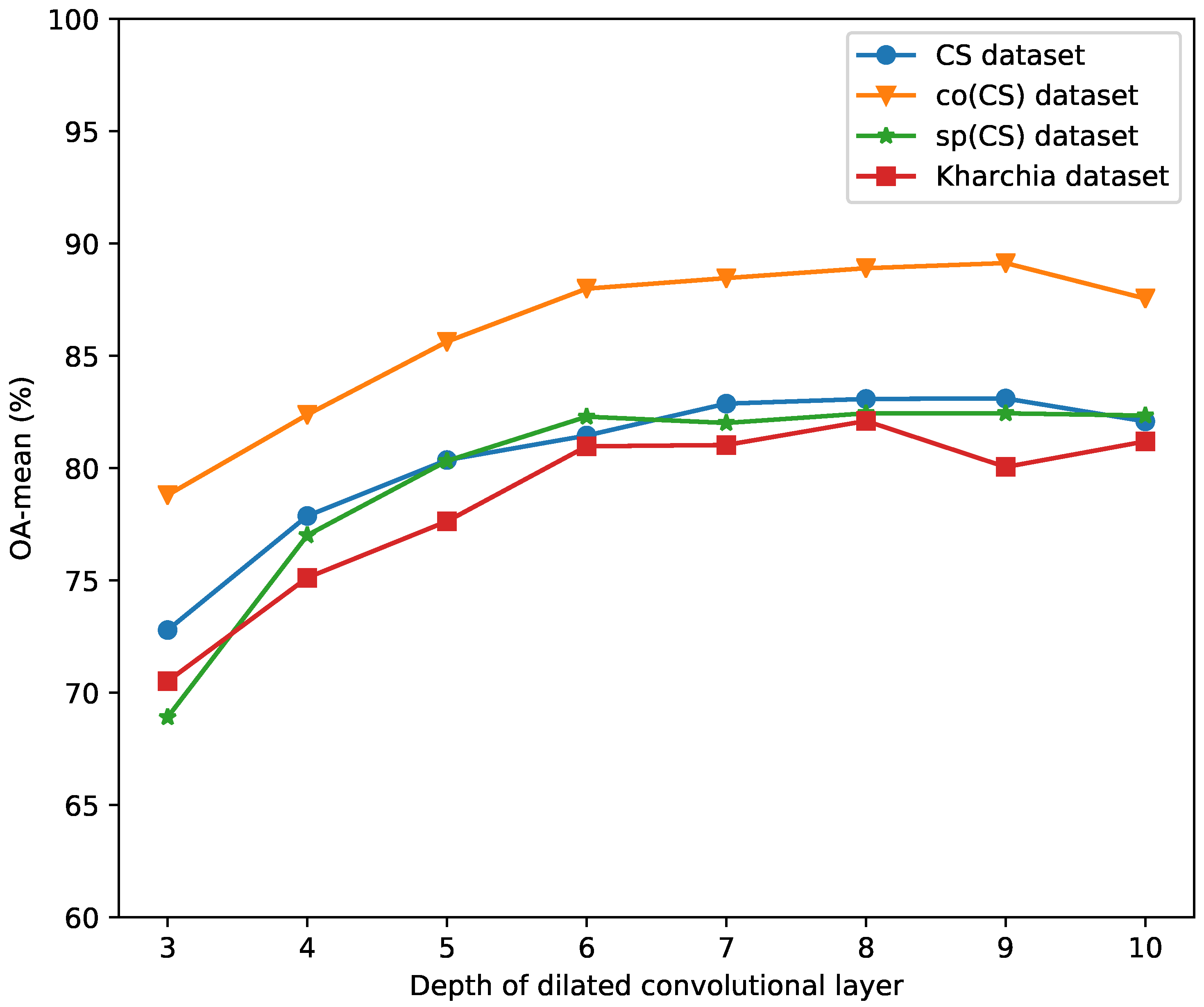
A quantitative analysis was performed to explore the dilated convolutional layers’ behaviour and obtain the optimum depth. Figure 5 shows the impact of the depth of the dilated convolutional layer on the performance (mean-OA). We assessed different numbers of N, from 3 to 10.

The figure shows that the impact of the depth on the performance behaviour is relatively similar for CS, co(CS), sp(CS), and Kharchia datasets. For a depth ranging from 3 to 6, the OA-mean increases sharply. The improvement drops from 6 to 7 and then relatively steady from the depth of 7. One possible reason is that those datasets have 215 bands. When N is 3, the global receptive field size, based on Equation (1), is $2^{3+1}-1=15$. The maximum dependency pattern the network can capture is only 15, while the data may have longer dependency patterns that have not been captured. Hence, the performance with $N=3$ is relatively low. Starting from a depth of 7 ($N=7$), the global receptive field size is $2^{7+1}-1=255$. The size is more than enough to capture the longest pattern in the data. When the depth is 8, most datasets reach the maximum performance. Increasing the depth beyond 8 does not significantly impact the performance. Sometimes, it can decrease the performance, e.g., the performance of the Kharchia dataset with a depth of 9 and CS and co(CS) with a depth of 10.

4.3. Ablation Analysis

4.3.1. Impact of Dilation on Performance

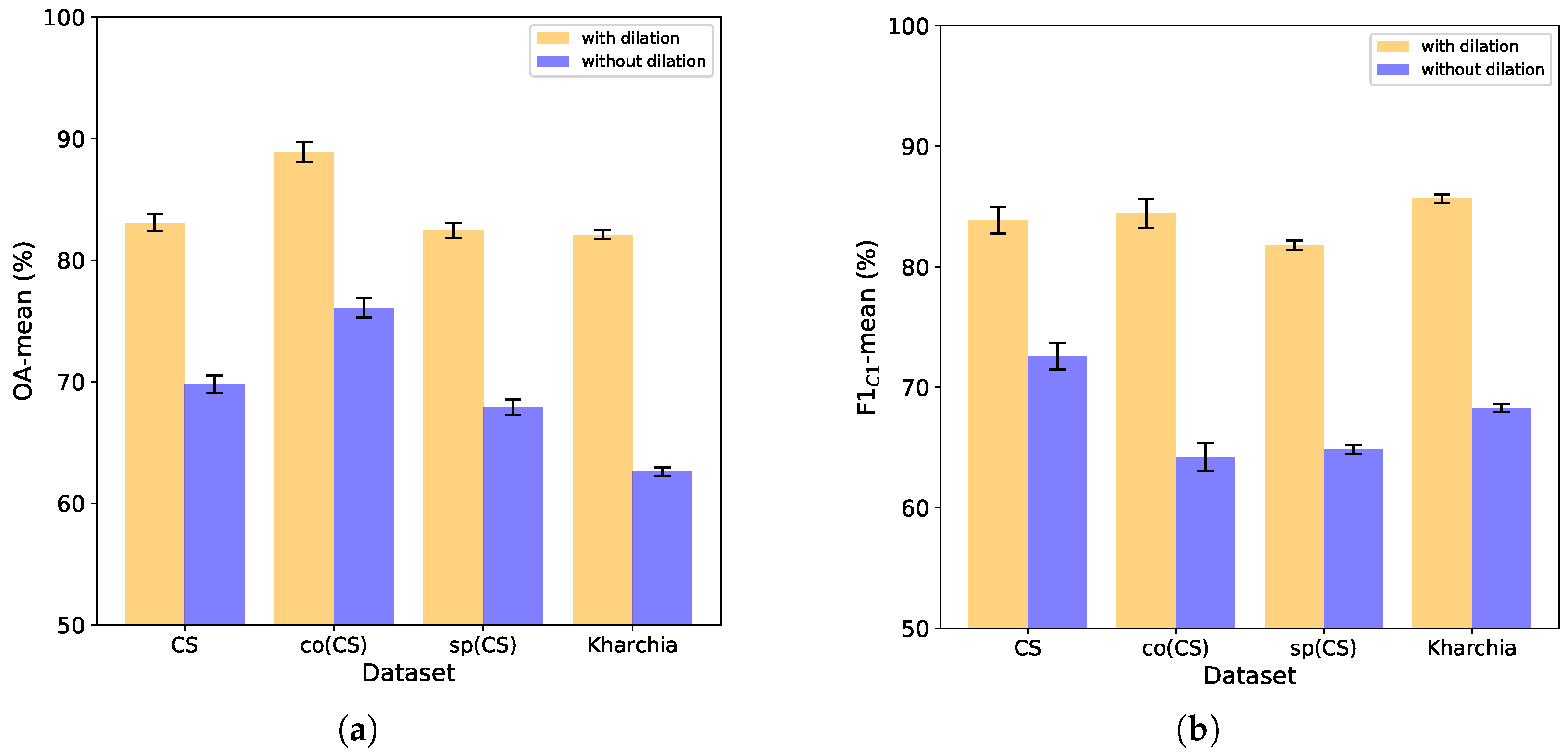
Using the optimal depth from the experiment in Section 4.2, i.e., 8, we evaluated the model performance for CS, co(CS), sp(CS), and Kharchia datasets for two scenarios: (i) model with dilation and (ii) model without dilation. In both scenarios, the architectures were the same, but for the model without dilation, a constant dilation rate of 1 was used instead of $2^{i-1}$ where i is the depth of the layer. Then, we reported OA-mean and F1_C1-mean produced by these two scenarios in Figure 6a,b. We presented OA results because OA has been widely used to interpret a model’s performance. However, OA does not take into account how the distribution of the predicted data. Hence, we also reported F1_C1 (F1 score of stressed salt) to interpret the precision and recall of the stressed salt (C1).

The dilated convolution enables the network to have a larger receptive field than the standard convolution, thereby enabling the capture of global features and longer dependencies between bands. As a result, dilated convolution is more suitable for hyperspectral data than the standard convolution when the network is shallow. It is clear that for all datasets, the OA-mean of the network with dilated convolutions is better by more than 10% (see Figure 6a). The F1_C1 of the network with dilated convolution is also superior by more than 10% to the respective model without dilation (see Figure 6b). The gap is higher, especially in the co(CS) dataset.

4.3.2. Impact of Channel Attention Module on Performance

Our ablation analysis (see

Table 1. Performance comparison between with and without channel attention module. The numbers in bold show the best performance.

Dataset	Performance	With Attention	Without Attention
CS	OA	83.08 ± 0.70	81.02 ± 2.79
	AA	83.15 ± 0.43	82.32 ± 1.61
	F1C0	82.21 ± 0.30	78.24 ± 5.96
	F1C1	83.86 ± 1.09	82.78 ± 1.94
co(CS)	OA	88.90 ± 0.81	85.24 ± 0.91
	AA	88.07 ± 0.88	84.01 ± 1.01
	F1C0	91.38 ± 0.62	88.11 ± 1.05
	F1C1	84.41 ± 1.17	80.46 ± 0.97
sp(CS)	OA	82.44 ± 0.62	79.73 ± 1.04
	AA	82.52 ± 0.52	80.20 ± 1.07
	F1C0	83.03 ± 1.09	80.93 ± 1.35
	F1C1	83.03 ± 1.09	78.22 ± 2.10
Kharchia	OA	82.10 ± 0.36	78.80 ± 2.09
	AA	81.25 ± 0.43	78.60 ± 2.00
	F1C0	76.23 ± 0.34	73.58 ± 1.22
	F1C1	85.65 ± 0.35	82.07 ± 3.15

) shows that channel attention enhances performance. The number of output channels for every dilated convolution layer in our network is C. Every convolutional layer will have C filters that work as feature descriptors to produce C channel-wise feature maps (C feature maps). Certain feature maps may not be essential or may contain little information that would not contribute much to the network. Intuitively, handling all the feature maps equally may hurt performance. Reported results show that weighting the feature maps based on their importance level improves the performance. The largest improvement is on AA of co(CS) dataset, which increases from 84.01% to 88.07% (4.06%), and the smallest improvement occurs in the AA of CS dataset with only 0.83%.

Table 1 shows that most measurements for the network without attention have larger standard deviations. For 5-fold experiments, one can conclude that the attention module improves the stability of the network.

4.4. Comparison with Existing Methods

This experiment compared our proposed architecture with several deep learning architectures and existing state-of-the-art methods for CS and Fusarium datasets. For CS, co(CS), sp(CS), and Kharchia datasets, we compared our model with a model that treated spectral information as a vector and used the standard 1D convolution to extract the features (1D CNN). We also compared the proposed method with the spectral-residual network (sRN), which uses 1D convolution and residual connections [53]. Furthermore, we compared our proposed method with methods that considered the spectral information as a sequence, e.g., RNN, LSTM [54] and spectralFormer [55]. We also compared our architecture with SFS Forward [10], the state-of-the-art method on the CS dataset.

For the Fusarium dataset, besides comparing our method with 1D CNN, LSTM [54], spectralFormer [55] and sRN [53], we also compared it with 2D-CNN-bidGRU [23] because it is the state-of-the-art method on the Fusarium dataset. Since the testing protocols, i.e., the training and testing sets, are different, we discarded samples that have zero values in all their bands while [23] did not; we report the results of 2D-CNN-bidGRU as reported in the paper [23] and 2D-CNN-bidGRU with our testing protocol to reflect the results with two testing protocols.

Table 2. Performance comparison between our proposed method and existing methods with CS, co(CS), sp(CS), and Kharchia datasets. The numbers in bold show the best performance.

Method	F1C0	F1C1	F1-mean	OA	AA
CS
1DCNN	71.40 ± 1.64	77.21 ± 0.46	74.31 ± 0.93	74.65 ± 0.79	74.50 ± 0.74
RNN	76.82 ± 2.68	80.02 ± 1.49	78.42 ± 1.96	78.57 ± 1.86	78.52 ± 1.89
LSTM	77.16 ± 0.88	81.27 ± 0.37	79.21 ± 0.60	79.42 ± 0.56	79.25 ± 0.54
sRN	79.78 ± 0.57	82.14 ± 0.95	80.97 ± 0.66	81.05 ± 0.69	80.98 ± 0.57
spectralFormer	77.55 ± 1.78	80.60 ± 0.96	79.08 ± 1.31	79.20 ± 1.26	79.09 ± 1.32
SFS_Forward	78.87	76.55	77.71	-	-
SC-CAN	82.21 ± 0.30	83.86 ± 1.09	83.03 ± 0.66	83.08 ± 0.70	83.15 ± 0.43
co(CS)
1DCNN	79.40 ± 0.51	61.84 ± 1.03	70.62 ± 0.73	73.25 ± 0.65	70.89 ± 0.72
RNN	82.20 ± 1.20	66.70 ± 2.75	74.45 ± 1.76	76.82 ± 1.47	74.98 ± 1.58
LSTM	84.36 ± 0.42	70.88 ± 0.98	77.62 ± 0.64	79.65 ± 0.54	78.05 ± 0.60
sRN	85.03 ± 0.65	70.74 ± 1.75	77.89 ± 1.05	80.20 ± 0.81	79.00 ± 0.97
spectralFormer	86.09 ± 1.03	73.88 ± 3.45	79.99 ± 2.21	81.86 ± 1.67	80.57 ± 1.52
SC-CAN	91.38 ± 0.62	84.41 ± 1.17	87.89 ± 0.89	88.90 ± 0.81	88.07 ± 0.88
sp(CS)
1DCNN	68.42 ± 0.63	65.32 ± 0.66	66.87 ± 0.57	66.95 ± 0.58	66.89 ± 0.58
RNN	79.31 ± 0.57	74.36 ± 1.38	76.83 ± 0.97	77.10 ± 0.89	77.57 ± 0.73
LSTM	76.07 ± 0.96	73.07 ± 1.26	74.57 ± 0.95	74.67 ± 0.94	74.70 ± 0.97
sRN	77.88 ± 0.53	74.70 ± 0.76	76.29 ± 0.47	76.41 ± 0.45	76.47 ± 0.44
spectralFormer	77.84 ± 1.45	75.21 ± 1.53	76.52 ± 1.22	76.62 ± 1.24	76.73 ± 1.33
SC-CAN	83.03 ± 1.09	81.78 ± 0.39	82.40 ± 0.60	82.44 ± 0.62	82.52 ± 0.52
Kharchia
1DCNN	53.46 ± 0.66	71.49 ± 0.59	62.47 ± 0.51	64.64 ± 0.54	62.55 ± 0.53
RNN	61.71 ± 4.56	80.44 ± 1.06	71.07 ± 2.38	74.18 ± 1.45	73.72 ± 1.66
LSTM	66.97 ± 0.98	79.91 ± 0.62	73.44 ± 0.74	75.02 ± 0.71	73.63 ± 0.75
sRN	69.71 ± 1.54	82.50 ± 0.73	76.11 ± 0.97	77.83 ± 0.85	76.87 ± 0.98
spectralFormer	67.57 ± 1.06	81.04 ± 1.22	74.30 ± 0.99	76.08 ± 1.13	74.93 ± 1.30
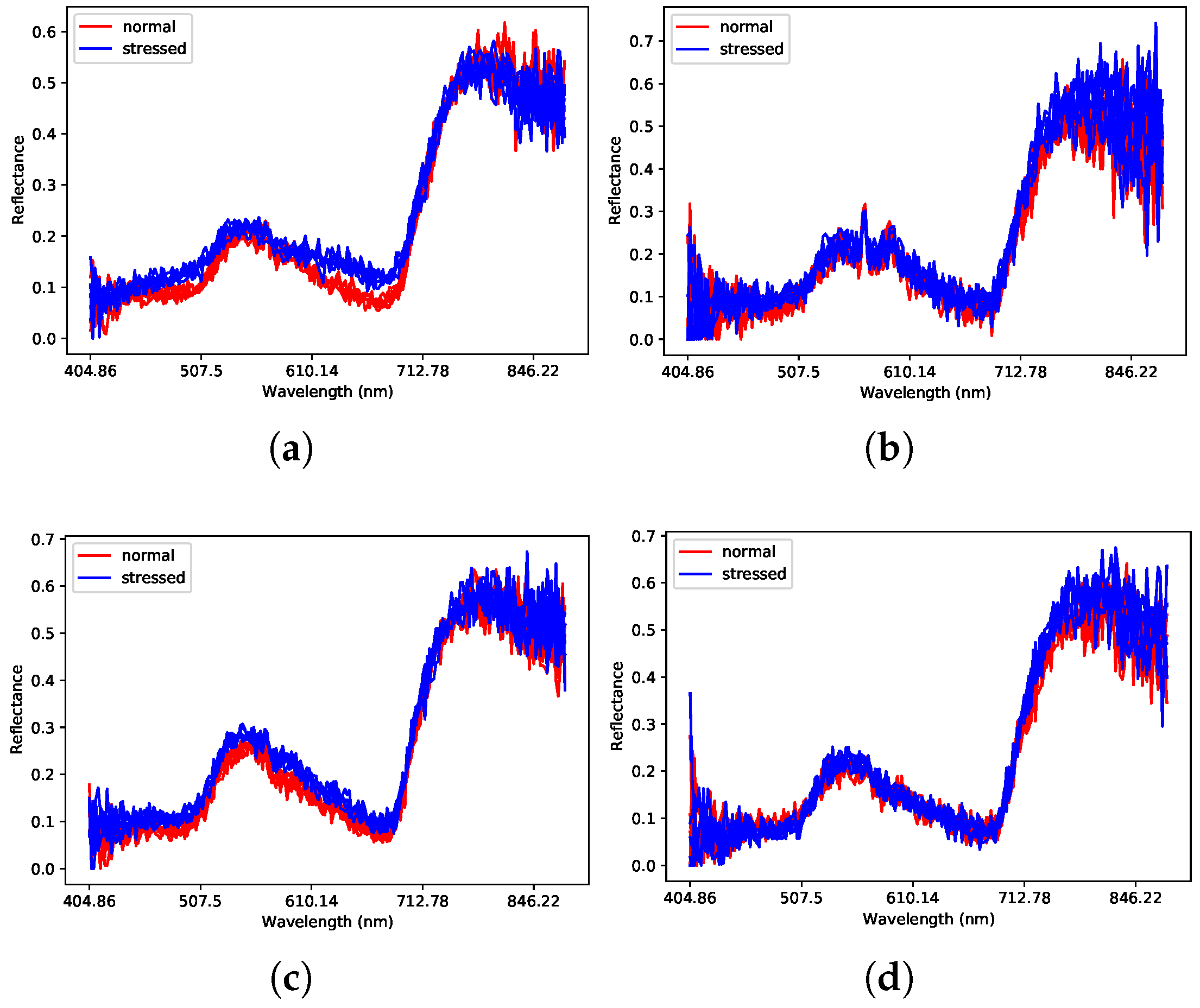
SC-CAN	76.23 ± 0.34	85.65 ± 0.35	80.94 ± 0.33	82.10 ± 0.36	81.25 ± 0.43

shows the performance comparison between our proposed method and existing methods with CS, co(CS), sp(CS), and Kharchia datasets. The table shows that the proposed method consistently produces the highest performance on all measurements and all datasets. Moreover, our proposed method outperforms SFS_Forward by a large margin of 7.31% in terms of F1_C1 on the CS dataset. We also find that compared to the baseline method, 1DCNN, adding spectral convolution and channel attention modules (in SC-CAN) improved the F1-score of class C1 (stressed salt) by 6.65%, 22.57%, 16.46%, and 14.16% for CS, co(CS), sp(CS), and Kharchia datasets, respectively. In comparing the performance of our proposed method across datasets, co(CS) dataset shows the best performance. Based on the visualization of normal and stress crop spectral reflectance from several samples in each dataset (as shown in Figure 7a–d), it is possible that the high performance of the co(CS) dataset is due to the lower inter-class similarity of the co(CS) dataset compared to the other datasets. The co(CS) dataset is therefore easier to classify.

Table 3. Performance comparison between our proposed method and existing methods with Fusarium dataset. The numbers in bold show the best performance.

Method	F1disease	F1healthy	F1background	OA	AA
1D CNN	52.71 ± 1.38	76.50 ± 0.29	79.21 ± 0.69	61.37 ± 33.89	62.58 ± 34.55
RNN	51.59 ± 8.29	83.27 ± 4.14	80.51 ± 1.77	79.79 ± 1.13	72.33 ± 3.46
LSTM	51.15 ± 4.57	77.35 ± 0.71	83.03 ± 1.54	78.36 ± 1.24	82.86 ± 0.65
sRN	39.78 ± 18.70	73.97 ± 14.35	77.56 ± 6.78	72.31 ± 11.68	76.09 ± 9.85
spectralFormer	62.99 ± 4.45	81.91 ± 0.61	84.18 ± 0.63	82.00 ± 0.89	72.59 ± 1.88
2D-CNN-BidGRU 1	52	71	88	74.30	-
2D-CNN-BidGRU 2	30.19 ± 0.85	62.30 ± 0.42	77.01 ± 0.26	66.70 ± 0.48	70.47 ± 0.19
SC-CAN	70.38 ± 3.10	83.25 ± 0.62	83.42 ± 1.68	82.78 ± 0.97	83.83 ± 1.65

¹ as reported in paper [23]; ² using our testing protocols.

presents the performance comparison between our proposed network and existing networks for the Fusarium head blight disease detection. The table shows that our proposed method produces the best results for F1_disease, OA, and AA. RNN produces a slightly better result for F1_healthy. The 2D-CNN-bidGRU produces a better result for F1_background than ours. However, we outperform 2D-CNN-bidGRU and RNN by a large margin for F1_disease. F1_disease and F1_healthy of SC-CAN outperform 2D-CNN-bidGRU by $\pm 18\%$ and $\pm 12\%$, respectively. Given that the Fusarium dataset is very imbalanced (the size of diseased-class samples is half of the size of background-class samples and a third of the size of healthy-class samples), and the upsampling process may produce noisy data, our proposed network still produces an acceptable result on F1_disease, i.e., 70.38%, compared to 52% from the result of 2D-CNN-bidGRU. This result shows that our proposed method is suitable for the case of an imbalanced dataset.

Three main reasons make the proposed SC-CAN method superior to other existing methods. First, our method is able to learn both local and global features, whereas 1D CNN and sRN, which are based on the standard convolution, are only capable of learning local features (see Section 3.1). Second, our method has a high model capacity because it exploits a large receptive field. As a consequence, unlike LSTM, our method can capture the long pattern dependencies of spectral information. Third our method pays more attention important feature maps.

5. Conclusions

We propose a novel architecture where spectral dilated convolutional layers extract spectral features for salt stress detection and Fusarium head blight disease classification from datasets that only have spectral information. By leveraging the spectral response of plants, our work can detect stress before visible symptoms appear. The key idea behind our method is the use of acausal dilated 1D convolution on the spectral vectors to capture the long dependencies between bands, local features, and global features. A channel attention module is also proposed to scale the channel-wise feature maps produced by spectral convolutional layers according to their importance. Experimental results demonstrate that the spectral dilated convolution and channel attention modules can improve the performance significantly. In addition, the channel attention network is also more stable than the respective network without channel attention modules. Based on the results of our experiments, our proposed network achieves state-of-the-art performance on CS, co(CS), sp(CS), Kharchia, and Fusarium datasets.

References

1. Sarwat, M.; Ahmad, A.; Abdin, M.Z.; Ibrahim, M.M. Stress Signaling in Plants: Genomics and Proteomics Perspective; Springer International Publishing: Cham, Switzerland, 2016; pp. 1–350. [Google Scholar] [CrossRef]
2. Suzuki, N.; Rivero, R.M.; Shulaev, V.; Blumwald, E.; Mittler, R. Abiotic and biotic stress combinations. New Phytol. 2014, 203, 32–43. [Google Scholar] [CrossRef] [PubMed]
3. Wang, Y.; Wang, H.; Peng, Z. Rice diseases detection and classification using attention based neural network and bayesian optimization. Expert Syst. Appl. 2021, 178, 114770. [Google Scholar] [CrossRef]
4. Chandel, N.S.; Chakraborty, S.K.; Rajwade, Y.A.; Dubey, K.; Tiwari, M.K.; Jat, D. Identifying crop water stress using deep learning models. Neural Comput. Appl. 2020, 33, 5353–5367. [Google Scholar] [CrossRef]
5. Mahlein, A.K. Plant Disease Detection by Imaging Sensors–Parallels and Specific Demands for Precision Agriculture and Plant Phenotyping. Plant Dis. 2016, 100, 241–251. [Google Scholar] [CrossRef]
6. Li, S.; Wu, H.; Wan, D.; Zhu, J. An effective feature selection method for hyperspectral image classification based on genetic algorithm and support vector machine. Knowl.-Based Syst. 2011, 24, 40–48. [Google Scholar] [CrossRef]
7. Audebert, N.; Le Saux, B.; Lefevre, S. Deep Learning for Classification of Hyperspectral Data: A Comparative Review. IEEE Geosci. Remote Sens. Mag. 2019, 7, 159–173. [Google Scholar] [CrossRef]
8. Huerta, E.B.; Duval, B.; Hao, J.K. Fuzzy Logic for Elimination of Redundant Information of Microarray Data. Genom. Proteom. Bioinform. 2008, 6, 61–73. [Google Scholar] [CrossRef]
9. Moghimi, A.; Yang, C.; Miller, M.E.; Kianian, S.F.; Marchetto, P.M. A Novel Approach to Assess Salt Stress Tolerance in Wheat Using Hyperspectral Imaging. Front. Plant Sci. 2018, 9, 1182. [Google Scholar] [CrossRef]
10. Moghimi, A.; Yang, C.; Marchetto, P.M. Ensemble Feature Selection for Plant Phenotyping: A Journey from Hyperspectral to Multispectral Imaging. IEEE Access 2018, 6, 56870–56884. [Google Scholar] [CrossRef]
11. Li, S.; Song, W.; Fang, L.; Chen, Y.; Ghamisi, P.; Benediktsson, J.A. Deep Learning for Hyperspectral Image Classification: An Overview. IEEE Trans. Geosci. Remote Sens. 2019, 57, 6690–6709. [Google Scholar] [CrossRef]
12. Shah, S.A.A.; Bennamoun, M.; Boussaïd, F. Iterative deep learning for image set based face and object recognition. Neurocomputing 2016, 174, 866–874. [Google Scholar] [CrossRef]
13. Graves, A.; Mohamed, A.R.; Hinton, G. Speech recognition with deep recurrent neural networks. In Proceedings of the ICASSP, IEEE International Conference on Acoustics, Speech and Signal Processing, Vancouver, BC, Canada, 26–31 May 2013; pp. 6645–6649. [Google Scholar]
14. Chow, V. Predicting auction price of vehicle license plate with deep recurrent neural network. Expert Syst. Appl. 2020, 142, 113008. [Google Scholar] [CrossRef]
15. Mou, L.; Ghamisi, P.; Zhu, X.X. Deep recurrent neural networks for hyperspectral image classification. IEEE Trans. Geosci. Remote Sens. 2017, 55, 3639–3655. [Google Scholar] [CrossRef]
16. Zhou, F.; Hang, R.; Liu, Q.; Yuan, X. Hyperspectral image classification using spectral-spatial LSTMs. Neurocomputing 2019, 328, 39–47. [Google Scholar] [CrossRef]
17. Hochreiter, S.; Bengio, Y.; Frasconi, P.; Schmidhuber, J. A field guide to dynamical recurrent neural networks. In Gradient Flow in Recurrent Nets: The Difficulty of Learning Long-Term Dependencies; Wiley-IEEE Press: Hoboken, NJ, USA, 2001; pp. 237–243. [Google Scholar]
18. Lipton, Z.C.; Berkowitz, J.; Elkan, C. A Critical Review of Recurrent Neural Networks for Sequence Learning. arXiv 2015, arXiv:1506.00019. [Google Scholar] [CrossRef]
19. Liu, Q.; Zhou, F.; Hang, R.; Yuan, X. Bidirectional-Convolutional LSTM Based Spectral-Spatial Feature Learning for Hyperspectral Image Classification. Remote Sens. 2017, 9, 1330. [Google Scholar] [CrossRef]
20. Lea, C.; Flynn, M.D.; Vidal, R.; Reiter, A.; Hager, G.D. Temporal Convolutional Networks for Action Segmentation and Detection. In Proceedings of the IEEE Conference on Computer Vision and Pattern Recognition (CVPR), Honolulu, HI, USA, 21–26 July 2017; pp. 156–165. [Google Scholar]
21. Hu, W.; Huang, Y.; Wei, L.; Zhang, F.; Li, H. Deep Convolutional Neural Networks for Hyperspectral Image Classification. J. Sens. 2015, 2015, 1–12. [Google Scholar] [CrossRef]
22. Peng, Z.; Huang, W.; Gu, S.; Xie, L.; Wang, Y.; Jiao, J.; Ye, Q. Conformer: Local Features Coupling Global Representations for Visual Recognition. In Proceedings of the IEEE/CVF International Conference on Computer Vision (ICCV), Montreal, BC, Canada, 11–17 October 2021; pp. 367–376. [Google Scholar]
23. Jin, X.; Jie, L.; Wang, S.; Qi, H.; Li, S. Classifying Wheat Hyperspectral Pixels of Healthy Heads and Fusarium Head Blight Disease Using a Deep Neural Network in the Wild Field. Remote Sens. 2018, 10, 395. [Google Scholar] [CrossRef]
24. Van Den Oord, A.; Dieleman, S.; Zen, H.; Simonyan, K.; Vinyals, O.; Graves, A.; Kalchbrenner, N.; Senior, A.W.; Kavukcuoglu, K. WaveNet: A generative model for raw audio. SSW 2016, 125, 2. [Google Scholar]
25. Zhu, L.; Li, C.; Wang, B.; Yuan, K.; Yang, Z. DCGSA: A global self-attention network with dilated convolution for crowd density map generating. Neurocomputing 2020, 378, 455–466. [Google Scholar] [CrossRef]
26. He, K.; Zhang, X.; Ren, S.; Sun, J. Deep residual learning for image recognition. In Proceedings of the IEEE Conference on Computer Vision and Pattern Recognition, Las Vegas, NV, USA, 27–30 June 2016; pp. 770–778. [Google Scholar]
27. Chen, L.; Zhang, H.; Xiao, J.; Nie, L.; Shao, J.; Liu, W.; Chua, T.S. SCA-CNN: Spatial and Channel-Wise Attention in Convolutional Networks for Image Captioning. In Proceedings of the IEEE Conference on Computer Vision and Pattern Recognition (CVPR), Honolulu, HI, USA, 21–26 July 2017. [Google Scholar]
28. Wang, J.; Jiang, T.; Cui, Z.; Cao, Z. Filter pruning with a feature map entropy importance criterion for convolution neural networks compressing. Neurocomputing 2021, 461, 41–54. [Google Scholar] [CrossRef]
29. Karlsson, I.; Friberg, H.; Kolseth, A.K.; Steinberg, C.; Persson, P. Agricultural factors affecting Fusarium communities in wheat kernels. Int. J. Food Microbiol. 2017, 252, 53–60. [Google Scholar] [CrossRef] [PubMed]
30. Peiris, K.H.S.; Dong, Y.; Davis, M.A.; Bockus, W.W.; Dowell, F.E. Estimation of the Deoxynivalenol and Moisture Contents of Bulk Wheat Grain Samples by FT-NIR Spectroscopy. Cereal Chem. J. 2017, 94, 677–682. [Google Scholar] [CrossRef]
31. Iliev, I.; Krezhova, D.; Yanev, T.; Kirova, E.; Alexieva, V. Response of chlorophyll fluorescence to salinity stress on the early growth stage of the soybean plants (Glycine max L.). In Proceedings of the RAST 2009—Proceedings of 4th International Conference on Recent Advances Space Technologies, Istanbul, Turkey, 11–13 June 2009; pp. 403–407. [Google Scholar] [CrossRef]
32. Hernández, E.I.; Melendez-Pastor, I.; Navarro-Pedreño, J.; Gómez, I. Spectral indices for the detection of salinity effects in melon plants. Sci. Agric. 2014, 71, 324–330. [Google Scholar] [CrossRef]
33. Hamzeh, S.; Naseri, A.A.; AlaviPanah, S.K.; Bartholomeus, H.; Herold, M. Assessing the accuracy of hyperspectral and multispectral satellite imagery for categorical and Quantitative mapping of salinity stress in sugarcane fields. Int. J. Appl. Earth Obs. Geoinf. 2016, 52, 412–421. [Google Scholar] [CrossRef]
34. Cao, F.; Guo, W. Deep hybrid dilated residual networks for hyperspectral image classification. Neurocomputing 2020, 384, 170–181. [Google Scholar] [CrossRef]
35. Pan, B.; Xu, X.; Shi, Z.; Zhang, N.; Luo, H.; Lan, X. DSSNet: A Simple Dilated Semantic Segmentation Network for Hyperspectral Imagery Classification. IEEE Geosci. Remote Sens. Lett. 2020, 17, 1968–1972. [Google Scholar] [CrossRef]
36. Pooja, K.; Nidamanuri, R.R.; Mishra, D. Multi-Scale Dilated Residual Convolutional Neural Network for Hyperspectral Image Classification. In Proceedings of the Workshop on Hyperspectral Image and Signal Processing, Evolution in Remote Sensing, Amsterdam, The Netherlands, 14–16 January 2019; Volume 2019, pp. 1–5. [Google Scholar]
37. Hamaguchi, R.; Fujita, A.; Nemoto, K.; Imaizumi, T.; Hikosaka, S. Effective Use of Dilated Convolutions for Segmenting Small Object Instances in Remote Sensing Imagery. In Proceedings of the 2018 IEEE Winter Conference on Applications of Computer Vision WACV, Lake Tahoe, NV, USA, 12–15 March 2018; Volume 2018, pp. 1442–1450. [Google Scholar]
38. Cotrozzi, L. Spectroscopic detection of forest diseases: A review (1970–2020). J. For. Res. 2022, 33, 21–38. [Google Scholar] [CrossRef]
39. Hou, J.; Wang, G.; Chen, X.; Xue, J.H.; Zhu, R.; Yang, H. Spatial-Temporal Attention Res-TCN for Skeleton-based Dynamic Hand Gesture Recognition. In Proceedings of the European Conference on Computer Vision (ECCV) Workshops, Munich, Germany, 8–14 September 2018. [Google Scholar]
40. Zagoruyko, S.; Komodakis, N. Paying more attention to attention: Improving the performance of convolutional neural networks via attention transfer. In Proceedings of the 5th International Conference on Learning Representations, ICLR 2017—Conference Track Proceedings, Toulon, France, 24–26 April 2017. [Google Scholar]
41. Vaswani, A.; Shazeer, N.; Parmar, N.; Uszkoreit, J.; Jones, L.; Gomez, A.N.; Kaiser, Ł.; Polosukhin, I. Attention is all you need. Adv. Neural Inf. Process. Syst. 2017, 30, 5999–6009. [Google Scholar]
42. Cheng, J.; Dong, L.; Lapata, M. Long Short-Term Memory-Networks for Machine Reading. In Proceedings of the EMNLP 2016—Conference on Empirical Methods in Natural Language Processing, Austin, TX, USA, 1–5 November 2016; pp. 551–561. [Google Scholar]
43. Lin, Z.; Feng, M.; dos Santos, C.N.; Yu, M.; Xiang, B.; Zhou, B.; Bengio, Y. A Structured Self-attentive Sentence Embedding. arXiv 2017, arXiv:1703.03130. [Google Scholar]
44. Parikh, A.P.; Täckström, O.; Das, D.; Uszkoreit, J. A Decomposable Attention Model for Natural Language Inference. In Proceedings of the EMNLP 2016—Conference on Empirical Methods in Natural Language Processing, Austin, TX, USA, 1–5 November 2016; pp. 2249–2255. [Google Scholar]
45. Mou, L.; Zhu, X.X. Learning to Pay Attention on Spectral Domain: A Spectral Attention Module-Based Convolutional Network for Hyperspectral Image Classification. IEEE Trans. Geosci. Remote Sens. 2020, 58, 110–122. [Google Scholar] [CrossRef]
46. Liu, Q.; Li, Z.; Shuai, S.; Sun, Q. Spectral group attention networks for hyperspectral image classification with spectral separability analysis. Infrared Phys. Technol. 2020, 108, 103340. [Google Scholar] [CrossRef]
47. Ribalta Lorenzo, P.; Tulczyjew, L.; Marcinkiewicz, M.; Nalepa, J. Hyperspectral Band Selection Using Attention-Based Convolutional Neural Networks. IEEE Access 2020, 8, 42384–42403. [Google Scholar] [CrossRef]
48. Woo, S.; Park, J.; Lee, J.Y.; Kweon, I.S. CBAM: Convolutional Block Attention Module. In Proceedings of the European Conference on Computer Vision (ECCV), Munich, Germany, 8–14 September 2018; pp. 3–19. [Google Scholar]
49. Guo, W.; Ye, H.; Cao, F. Feature-Grouped Network with Spectral-Spatial Connected Attention for Hyperspectral Image Classification. IEEE Trans. Geosci. Remote Sens. 2022, 60, 5500413. [Google Scholar] [CrossRef]
50. Zhu, X.; Cheng, D.; Zhang, Z.; Lin, S.; Dai, J. An Empirical Study of Spatial Attention Mechanisms in Deep Networks. In Proceedings of the IEEE/CVF International Conference on Computer Vision (ICCV), Seoul, Korea, 27 October–2 November 2019. [Google Scholar]
51. Farha, Y.A.; Gall, J. MS-TCN: Multi-stage temporal convolutional network for action segmentation. In Proceedings of the IEEE/CVF Conference on Computer Vision and Pattern Recognition (CVPR), Long Beach, CA, USA, 15–20 June 2019. [Google Scholar]
52. van den Oord, A.; Kalchbrenner, N.; Vinyals, O.; Espeholt, L.; Graves, A.; Kavukcuoglu, K. Conditional Image Generation with PixelCNN Decoders. Adv. Neural Inf. Process. Syst. 2016, 29, 4797–4805. [Google Scholar]
53. Khotimah, W.N.; Bennamoun, M.; Boussaid, F.; Sohel, F.; Edwards, D. A high-performance spectral-spatial residual network for hyperspectral image classification with small training data. Remote Sens. 2020, 12, 3137. [Google Scholar] [CrossRef]
54. Xu, Y.; Zhang, L.; Du, B.; Zhang, F. Spectral-Spatial Unified Networks for Hyperspectral Image Classification. IEEE Trans. Geosci. Remote Sens. 2018, 56, 5893–5909. [Google Scholar] [CrossRef]
55. Hong, D.; Han, Z.; Yao, J.; Gao, L.; Zhang, B.; Plaza, A.; Chanussot, J. SpectralFormer: Rethinking Hyperspectral Image Classification with Transformers. IEEE Trans. Geosci. Remote Sens. 2021, 60, 5518615. [Google Scholar] [CrossRef]
Figure 1. (a) An example of standard spectral convolution, and (b) An example of dilated spectral convolution, where the receptive field is much larger with just few layers.
Remotesensing 14 04288 g001
Figure 2. (a) Overview of the proposed network, (b) the detail of a spectral convolution module, which consists of a dilated convolutional layer that residually connected and has two activation functions, “ t a n h ” and “ σ ” (sigmoid), and (c) the architecture of a channel attention module, which utilizes global average pooling along the spectral axis and fully connected layers to compute inter-relationship between channel-wise feature maps.
Remotesensing 14 04288 g002
Figure 3. Convolution process with input spectral signal and a kernel size of 3 to produce local features.
Remotesensing 14 04288 g003
Figure 4. (a) An example of causal dilated convolutions, where the convolution output of a certain band does not depend on the information of the next bands and (b) an example of acausal dilated convolution, where the convolution output of a certain band depends on the information of the adjacent bands.
Remotesensing 14 04288 g004
Figure 5. Performance comparison of our proposed method for different numbers of dilated convolutional layers. OA-mean is the average of OA from 5-fold experiments.
Remotesensing 14 04288 g005
Figure 6. Performance comparison (a) OA-mean and (b) F1C1 between dilated convolution and standard convolution in our proposed architecture. Note: the values are averaged from 5-fold experiments.
Remotesensing 14 04288 g006
Figure 7. The spectral signal visualization from several samples (a) Example signal of healthy and salt stressed crops from co(CS) (b) CS, (c) sp(CS), and (d) Kharchia datasets.
Remotesensing 14 04288 g007