Article

A Batch Pixel-Based Algorithm to Composite Landsat Time Series Images

1
School of Geography and Tourism, Anhui Normal University, Wuhu 241003, China
2
Engineering Technology Research Center of Resources Environment and GIS, Anhui Province, Wuhu 241003, China
3
Collection and Editing Department of Library, Wannan Medical College, Wuhu 241003, China
*
Author to whom correspondence should be addressed.
Remote Sens. 2022, 14(17), 4252; https://doi.org/10.3390/rs14174252
Submission received: 24 June 2022 / Revised: 9 August 2022 / Accepted: 25 August 2022 / Published: 29 August 2022
(This article belongs to the Section Remote Sensing Image Processing)

Abstract

:
Compositing is a fundamental pre-processing for remote sensing images. Landsat series optical satellite images are influenced by cloud coverage, acquisition time, sensor types, and seasons, which make it difficult to obtain continuous cloud-free observations. It limits the potential use and analysis of time series images. Therefore, global change researchers urgently need to ‘composite’ multi-sensor and multi-temporal images. Many previous studies have used isolated pixel-based algorithms to composite Landsat images; however, this study is different and develops a batch pixel-based algorithm for composing continuous cloud-free Landsat images. The algorithm chooses the best scene as the reference image using the user-specified image ID or related parameters. Further, it accepts all valid pixels in the reference image as the main part of the result and develops a priority coefficient model. Development of this model is based on the criteria of five factors including cloud coverage, acquisition time, acquisition year, observation seasons, and sensor types to select substitutions for the missing pixels in batches and to merge them into the final composition. This proposed batch pixel-based algorithm may provide reasonable compositing results on the basis of the experimental test results of all Landsat 8 images in 2019 and the visualization results of 12 locations in 2020. In comparison with the isolated pixel-based algorithms, our algorithm eliminates band dispersion, requires fewer images, and enhances the composition’s pixel concentration considerably. The algorithm provides a complete and practical framework for time series image processing for Landsat series satellites, and has the potential to be applied to other optical satellite images as well.

Graphical Abstract

1. Introduction

More than 8 million scenes have been gathered in Landsat series satellite data; this number is increasing at a rate of more than 400,000 scenes each year [1]. These bring considerable differences in many scientific communities [2], such as climate change, fire outbreaks, and landscape monitoring [3,4,5]. However, because of the massive amount of data, it is difficult to easily gather, handle, and evaluate. Therefore, automatic processing techniques are necessary [6].
Landsat offers almost 50 years of continuous observations with a free data access policy [7] for long-term remote sensing applications and global change studies. Therefore, multi-sensor and multi-temporal images should be composited to provide continuous sky-clear time series images [8,9]. Pixel-based image compositing is replacing traditional scene-based compositing [10] because of the creation of cloud-free, radiometric, and phenology-consistent image composites that are continuous over large areas depending on the set of user-defined criteria [11]. The average number of Landsat images included in the analysis increased from 10 in 2008 to 100,000 in 2020 [9], and the successful launch and application of Landsat 9 doubled the temporal resolution of the Landsat series satellites [1,12]. Based on such developments, dozens of new studies are conducted, which are providing humankind with a better understanding of the planet and human activities. Forests [13], agricultural mapping [14], water management [15], land cover/land change [16], disasters [17], climate monitoring [4], and environmental conservation [18] are among the research fields in which Landsat data and data processing algorithms play important roles. Furthermore, frequently, there are specific restrictions on the lengths of the observation times in practical analyses. For example, the observation period for the study of the reaction of ecological vegetation to natural floods is limited to 1–3 months [19]. In the study of a forest fire assessment, there is a need to determine the narrow period before and after the fire event [20]. However, due to Landsat’s poor temporal resolution and uncertain high cloud coverage, it is challenging to obtain the desired images within the required time frame.
Not only do enormous amounts of data and multiple sensors need image compositions, a wide range of requirements also need better compositing algorithms.
For the study of image compositing algorithms, earlier compositing methods were only developed for coarse resolution sensors, such as AVHRR [21] and MODIS [22]. However, these algorithms are not suitable for Landsat data since the sensor has a small field of view of 15 and the repeat cycle is 16 days. Therefore, Landsat data do not provide sufficient numbers or angles of surface samplings to invert the bidirectional reflection models [23]. Fortunately, few studies were conducted about Landsat in recent years. Roy et al. [24] were the first to propose an image composite approach for Landsat ETM+ data, primarily based on a combination of maximum NDVI and the greatest brightness temperature criteria. This benchmark work has been applied in the United States and the final composites are available for free download. Potapov et al. [25] used median values of the near-infrared (NIR) band as the criteria to choose the best data; this method outperformed the standard maximum NDVI compositing method. Griffiths et al. [26] created a mechanism for calculating scores for each Landsat observation, with image compositing criteria set by weighted scores that were generated based on acquisition year, acquisition day of the year, and distance of a specific pixel to the cloud. Furthermore, White et al. [11] developed a pixel-based image compositing approach based on the sensor type, day of year, distance to the cloud, or cloud shadow and opacity. Zhu et al. [27] proposed estimating time series models for each pixel and spectral band using all available clear Landsat observations to forecast daily compositing Landsat images. Google Earth Engine (GEE) is a cloud computing platform that provides massive satellite data processing interfaces and algorithms, including Landsat. It implements a general algorithm known as median [28], based on Potapov’s [25] ideas, as well as a composition algorithm for Landsat called ‘SimpleComposite’ [28] (referred to as simple), which integrates the ideas by White [11] and Roy [24].
However, there are two huge difficulties with the algorithms mentioned above. First, it is uncertain whether to evaluate the different compositing results quantitatively. Most evaluations rely on visual inspections of natural color composites due to the lack of a standard set of reference images for comparison [8]. Second, isolated pixel-based algorithms are unconcerned about the association of pixels on the same image, which may lead to a temporal or band dispersion of pixels in the compositing results.
In this study, a batch pixel-based composition algorithm is proposed for a temporal or band dispersion of compositing results by taking five factors into account, including cloud coverage, observation time, acquisition year, observation season, and sensor types. Furthermore, rather than the traditional visual inspection, temporal dispersion is provided, which is used as an indicator to quantitatively evaluate the compositing results. This research may help to understand the cloud removal processing in a better way and create a more reasonable composition algorithm for Landsat time series images.
The structure of this paper is organized as follows. Following the introduction, Section 2 describes research materials and main details of the new batch pixel-based composite algorithm (referred to as batch). Section 3 describes the research results and compares the differences between the algorithm in this study and the median and simple algorithms provided by GEE using all Landsat 8 satellite observations in 2019 as sample data. Section 4 describes the advantages and shortcomings of this algorithm and Section 5 provides a summary of the study.

2. Materials and Methods

2.1. Data

The remote sensing data used in this study were all collected from GEE. They include Landsat 4, 5, 7, 8 in the Landsat series. Observations of Landsat 1, 2, 3 are also available but these were not considered due to the low quality and small amounts of observations, which could limit the feasibility of the application [29].
Three online sensors, ETM+ of Landsat 7, OLI of Landsat 8, and OLI2 of Landsat 9 continually contribute fresh observations, as shown in Figure 1. These summarize and illustrate the sources and timeliness of the data, which are now accessible on the GEE platform. For Landsat 7 and Landsat 8, there are around 1200 new images added per day [2], and Landsat 9 provides 740 new scenes per day [12]. It is expected that the GEE platform will soon provide these images as well as the accessibility to the general public.
In this study, all high-quality observations (the image attribute I M A G E _ Q U A L I T Y equals 9) of Landsat 8 worldwide between 1 January 2019 and 31 December 2019 were collected as test sample data. These are fairly distributed over global land areas with different latitudes and longitudes, seasons, and ecological zones for which batch, median, and simple compositing algorithms are performed at each location to obtain more reliable statistical data for comparisons.
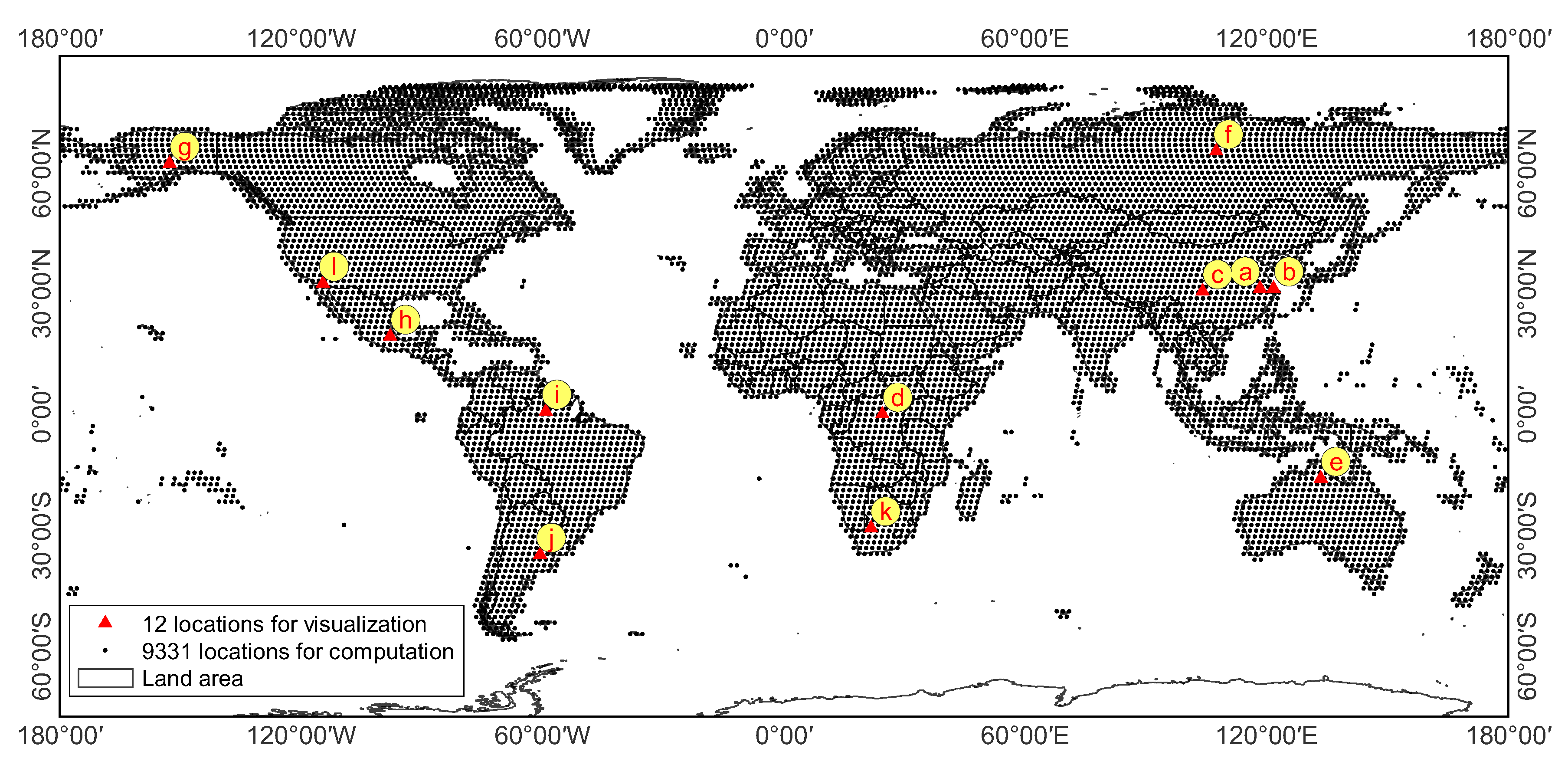
At the same time, twelve visualization locations of interest were selected at various latitudes and cloud coverage zones (Table A1 and Figure 2). The data acquisition time range of the visualization points was restricted between 1 May and 30 September 2020. Visual data have different date ranges than test data. The first involves limiting the scenes of available images to overcome the cloud coverage disturbance and the second to check the performances in various years. A square buffer as a mask within 5 km was used, centered on the corresponding location for image cropping. For better image details, a small buffer distance is used to reduce the field of vision (such as moving ships).

2.2. Method

2.2.1. Automated Algorithm for the Batch Composition

The batch pixel-based composition algorithm proposed in this study consists of three steps (Figure 3): (1) Calculation of the reference image to obtain the main part of the compositing result; (2) Calculation of the priority index based on the combined five factors to obtain the missing part in order of priority; (3) Composition of the main and missing parts into one image.

2.2.2. Reference Image

The reference image is the image that the user believes to be the best, which constitutes the majority of the final compositing result. It can be selected automatically from a set of images that fit the user input parameters or it can be uniquely defined by specifying an image ID. The following represents its computational logic: the user-specified image ID is preferred as the reference image; however, if it is not specified, then images are first matched according to the user-specified year, season and sensor types. Likewise, the set of matched images is sorted according to the amount of cloud coverage and finally the one with the least amount of clouds is specified as the reference image. After removing the cloud, cloud shadow, and invalid pixels [30] from the reference image, the part that remains is the main part of the compositing result. The rest of the part, other than the main part, is considered the missing part. All available observations except the reference image, including the available sensor types, years, and seasons, might be used to fill the missing part.

2.2.3. Priority Index

The purpose of the priority index is to find the optimal substitute for the missing pixels. To calculate the priority of the substitute, a criterion based on five priorities is defined.
(1)
The smaller the observation date difference between the substitute and the reference image, the higher the priority;
(2)
The smaller the acquisition year difference between the substitute and the reference image, the higher the priority;
(3)
Less cloud coverage;
(4)
Images from the same season;
(5)
Images from the same sensor type.
Based on the aforementioned criteria, the priority index is defined as follows.
v = β × i = 1 5 α i v i 2 / i = 1 5 α i ( v , v i [ 0 , 1 ] ; α i , β { 0 , 1 } )
where v is the priority index with the value range of [0,1] and β is the overall quality control coefficient of the remote sensing image, which is used to filter the observations with the poor overall image quality. When the observation parameter I M A G E _ Q U A L I T Y is 9, β = 1 , otherwise it is considered as β = 0 . v i is the ith priority factor of the above-mentioned five priority factors, and α i is the weight of the corresponding ith priority factor, which is used to control whether the factor participates in the calculation of the priority index or not. α i takes the value of 0 or 1. The value of 1 means that the corresponding factor participates in the priority index calculation; otherwise, it does not.
The detailed calculation method of each priority factor is as follows.
v 1 = 1 d x d 0 365 ( v 1 [ 0 , 1 ] ; d 0 , d x [ 1 , 365 ] )
where, d x and d 0 are the DOY attribute of the computed image and the reference image, respectively.
v 2 = 1 c x c 0 100 ( v 2 [ 0 , 1 ] ; c 0 , c x [ 0 , 100 ] )
where c x and c 0 are the C L O U D _ C O V E R attribute of the computed image and the reference image, respectively.
v 3 = 1 5 y x y 0 ( v 3 [ 0 , 1 ] )
where y x and y 0 are the acquisition years of the computed image and the reference image, respectively. The larger the distance between the two, the lower the priority level. Since the Food and Agriculture Organization of the United Nations uses a five-year criteria for land use management [31], the power function with a base of 0.2 can better describe the priority of various years.In the function, the current year’s maximum priority value is 1. The priority value declines dramatically with the distance deviation, tending to 0 after more than 4 years.
v 4 = 1 , s e a s o n x = s e a s o n 0 0 , s e a s o n x s e a s o n 0 ( v 4 { 0 , 1 } )
where s e a s o n x and s e a s o n 0 are the acquisition seasons of the computed images and the reference images, respectively.
v 5 = 1 , s e n s o r x = s e n s o r 0 0 , s e n s o r x s e n s o r 0 ( v 5 { 0 , 1 } )
where s e n s o r x and s e n s o r 0 are the satellite sensor types of the computed images and reference images, respectively.

2.2.4. Composition Properties

To describe the status of the original image data, some attributes are attached to the compositing results, which include the following:
(a)
The compositing integrity;
(b)
The number of scenes used in the composition, which corresponds to the temporal dispersion;
(c)
The time and contribution ratio of each scene used in the composition;
(d)
Whether the compositing integrity is achieved or not.
The definition of integrity is:
I n t e g r i t y = 1 n l o s s / n a l l
where I n t e g r i t y is the compositing integrity. n l o s s and n a l l are the number of missing pixels and total pixels of the image respectively, whereas the former is divided by the latter to obtain the missing percentage. The compositing success rate can be described as:
S u c c e s s = c o u n t s u c c e s s / C o u n t a l l
where S u c c e s s is the compositing success rate. Successful composition depends on the integrity objective (The integrity objective is a user-defined threshold. A total of six thresholds are used in this study, which are 90 % , 95 % , 99 % , 99.9 % , 99.99 % , and 99.999 % , respectively.). If the compositing result meets the integrity objective it is considered a successful composition; otherwise, it is considered a failed composition. c o u n t s u c c e s s and c o u n t a l l represent the number of successful and total observations for a given PATH/ROW. For all of the positions with successful compositions, the required scene count is aggregated. According to the data characteristics, the required scenes count is divided into six groups: 1–1, 2–3, 4–6, 7–11, and >=12. The average cloud coverage of each group is calculated.

2.2.5. Methods of Sampling and Comparison

To visually quantify the differences between different methods, several commonly used indices, such as NDVI [32], NDBI [33], and NDWI [34] are generated by band computations, which are widely used to express vegetation, built-up areas, and water separately. The following are the definitions for the indices mentioned above:
N D V I = ( N I R R e d ) ( N I R + R e d )
N D B I = ( S W I R N I R ) ( S W I R + N I R )
N D W I = ( G r e e n N I R ) ( G r e e n + N I R )
where N I R , R e d , S W I R , and G r e e n are the reflectance of digital values of the Landsat images’ near-infrared band, red band, mid-infrared band, and green band, respectively.
After generating the three remote sensing indices as mentioned earlier, 5000 pixels are chosen randomly for comparison from the compositing results of the 12 visualization locations listed in Table A1 and Figure 2.

2.2.6. Implementation and Source Code of the Algorithm

The automated batch pixel-based Landsat image compositing algorithm has been implemented and released as a GEE application. It provides compositions for Landsat images from the previous 40 years throughout the world and nine kinds of vegetation index (VI) products such as NDVI, NDWI, NDBI, and so on. Furthermore, all outputs can be easily compared to isolated pixel-based algorithms, such as the median and simple, and differences can be seen in algorithm outputs. The source code and documentation for the GEE implementation are available at https://leejianzhou2080.users.earthengine.app/view/referencecomposite (accessed on 20 December 2021). In addition, we made all intermediate data used in the application available to the public. Users are encouraged to adopt our techniques to produce compositing products using remote sensing data.

3. Results

3.1. Spatial Distribution of Observation Frequencies and Cloud Coverage

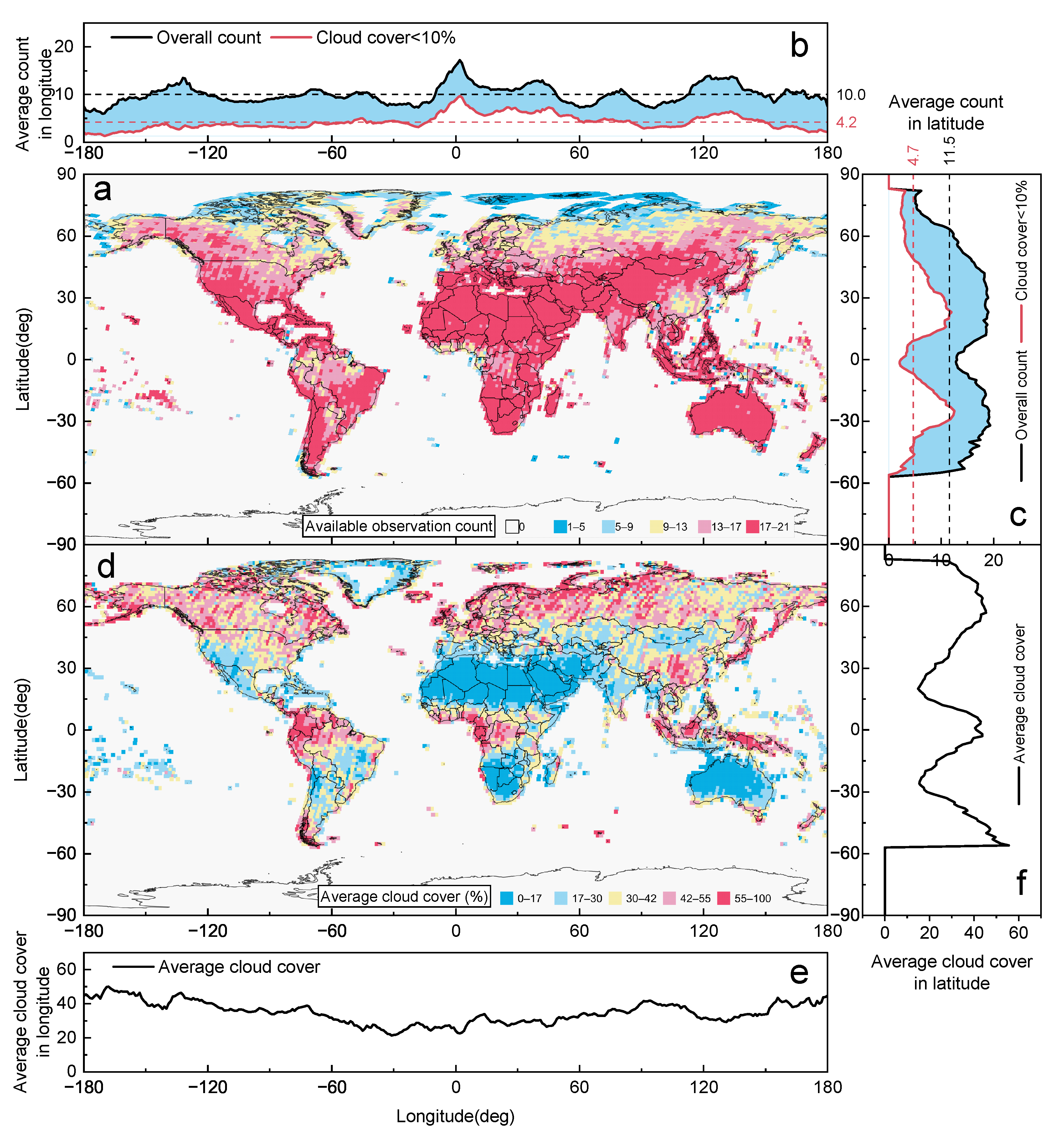
Landsat 8 had a total of 137,594 high-quality scenes in 2019, distributed over 9331 sites (Figure 4a–c), with an average of 14.7 high-quality images per site. However, the spatial distribution varied widely, with high latitudes and polar regions being significantly lower than low and middle latitudes. The average number of observations at different latitudes was 11.5; in the Arctic, this number dropped below 5. In Antarctica, there are no available observations. This implies that different strategies are needed in different regions: polar regions need to lower both compositing integrity and success rate expectations and high latitudes need to lower integrity appropriately.
The management of cloud coverage is pivotal in remote sensing image composition. It is one of the biggest obstacles in image processing [35]. With an average cloud coverage of 31.5% ± 30.9% during 2019, Figure 4d–f show generally large cloud coverage and a wide range of variability. The frequency of observations with less than 10% cloud coverage is much lower than the total frequency of observations (the magenta lines in Figure 4e,f), and the average values in longitude and latitude directions are 4.2 and 4.7, respectively, accounting for less than 30% of the total average observations.

3.2. Global Comparison of the Three Composition Algorithms

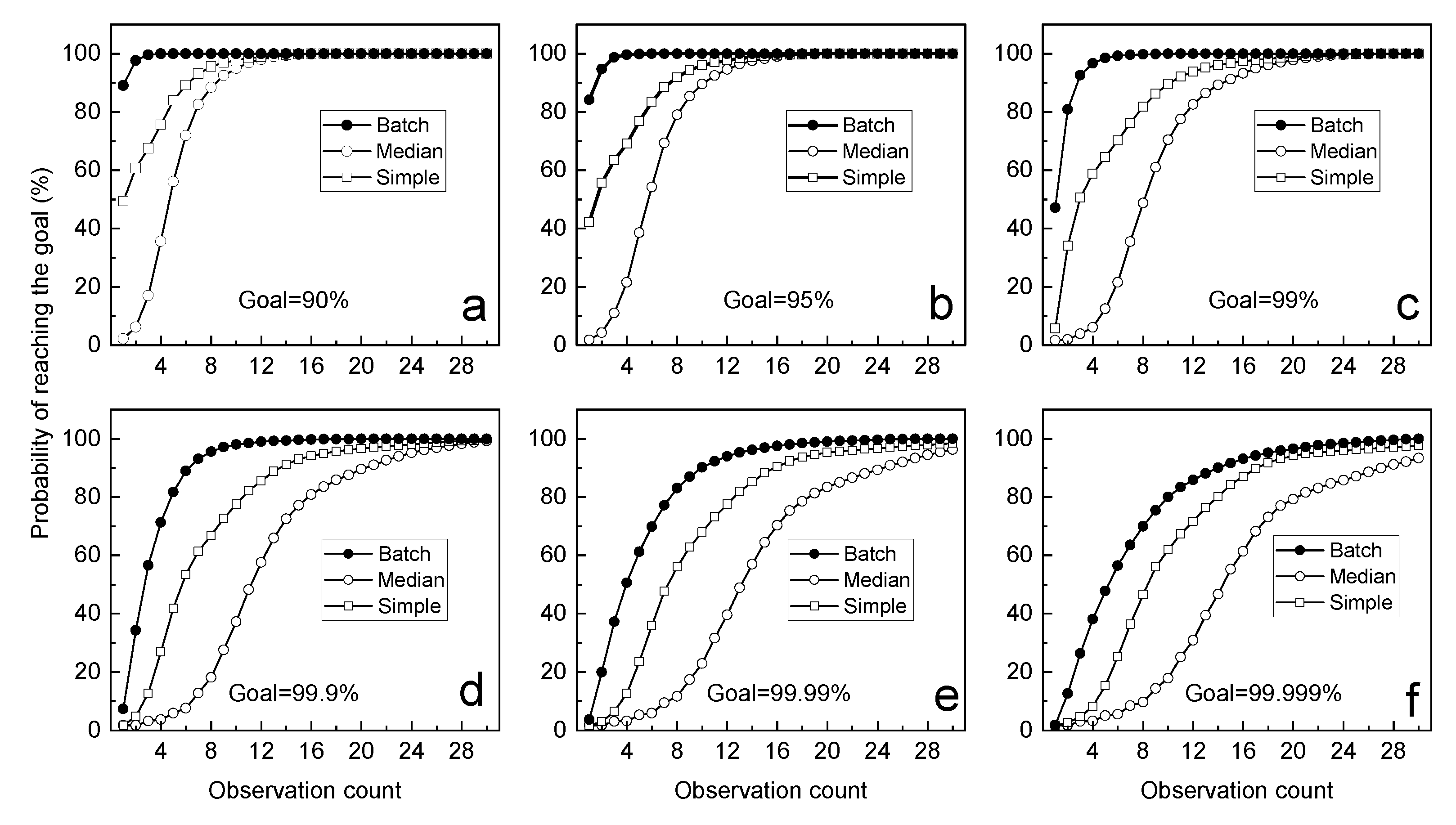
To investigate the differences in integrity and success rates of the three compositing algorithms, six different compositing integrity goals are set ranging from 0.9 to 0.99999. To achieve the targeted integrity, compositing calculations are performed for 9331 observed locations with a limit of a maximum of 30 images of each location through the batch, median, and simple algorithms. Figure 5 and Table A2 show the relationship between compositing integrity and success rate.
From the results, the performance of the batch algorithm is far better than the median and simple algorithms. Taking the first integrity goal as an example (90%, Figure 5a), the compositing results of the top three images are significantly different: (1) If the three methods only use one image, the success rates of the batch, median, and simple algorithms are 89.1%, 49.3%, and 2.2 % , respectively; (2) With the use of two images, the success rate of the batch algorithm increases to 97.7% while the median and simple increase to 60.7% and 6.2%, respectively; (3) With the use of three images, the success rate of the batch algorithm reaches 99.997% while the median and simple are far lower than this value. The results are similar for other integrity goals as well (Figure 5b–f).
The use of fewer observations gives larger concentrations of data as a result. The use of one scene with 100% integrity can give the ideal result to the user. However, in practice, it is frequently not possible, and the greater the integrity requirement, the more observations are used, and vice versa. Our experimental results show less than 2% possibility to achieve 99.999% integrity with one scene (Table A2). After looking at the difficulties in obtaining 100% integrity in realistic data processing, 99% integrity seems to be a better compromising option. As a result, Figure 6 shows the geographical distribution of the number of observations needed by the various algorithms to achieve 99% integrity. The batch algorithm requires just three observations to achieve the 99% integrity goal for the majority of sites (blue region in Figure 6a); however, the median and simple algorithms require much greater frequency. On the other hand, larger frequencies are primarily found in coastal and inland basin areas (the red areas in Figure 6a), indicating that more observations are needed in places where cloud cover is more. According to the relationship between the required count and cloud cover in Figure 7, the batch method’s average cloud coverage grows as the required image count rises. It demonstrates that it can discriminate between various observations and the processing of cloud coverage is more logical.
We may have more strict observation period requirements in practical analyses, such as in studies of forest fires [36,37] and floods [3], where the research duration is generally limited to 1–2 months. Table 1 shows the compositing success rate using the three algorithms when the observation duration is restricted to about 2 months. If the user requires 90% integrity, the batch method has a success rate of 99.9%, whereas if the user requires 99% integrity, the batch has a success rate of 96.6%.
The batch pixel-based algorithm in this study has a substantially better compositing success rate than the isolated pixel-based algorithm, and significantly reduces the number of necessary satellite observations.

3.3. Visualization Results of Different Algorithms

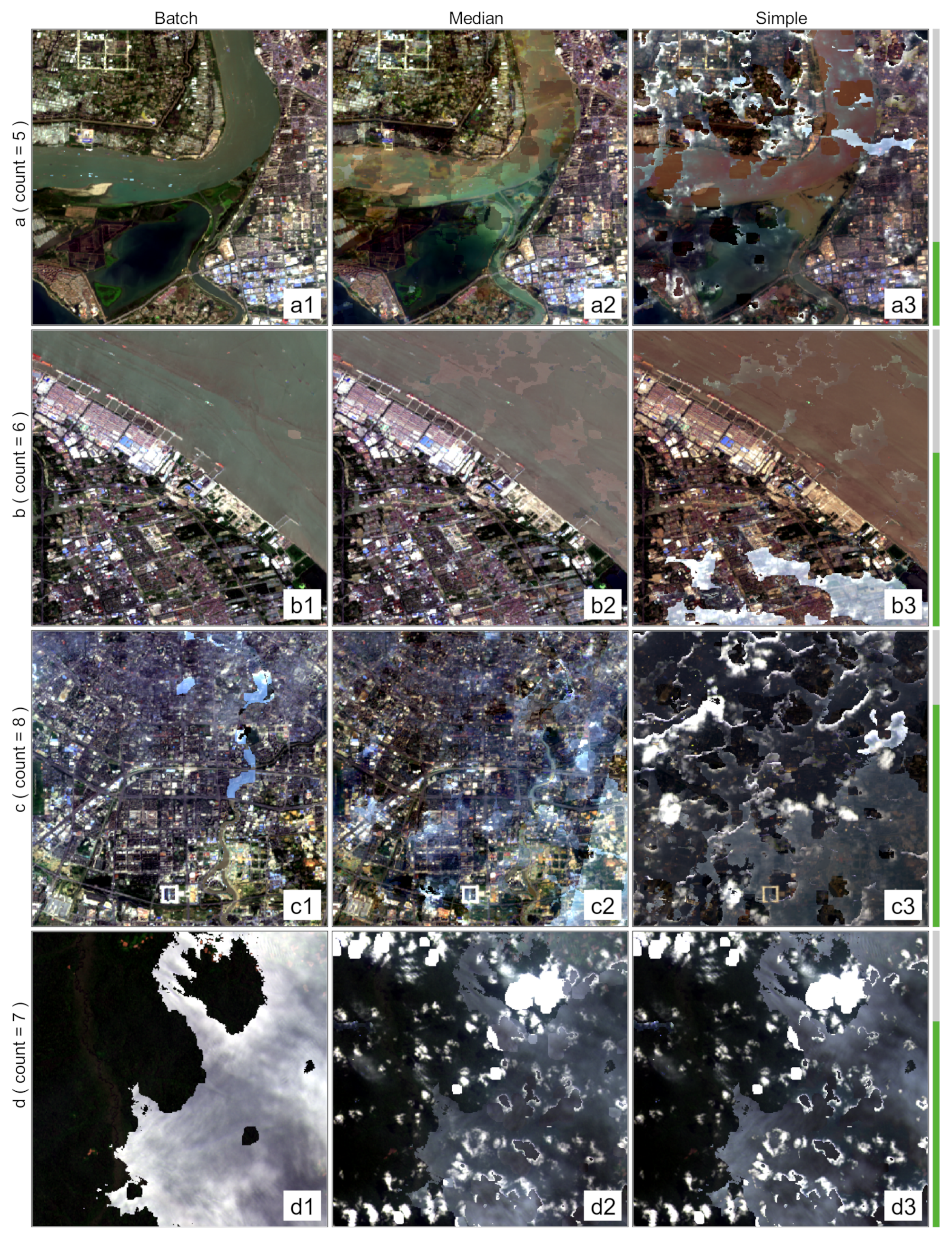
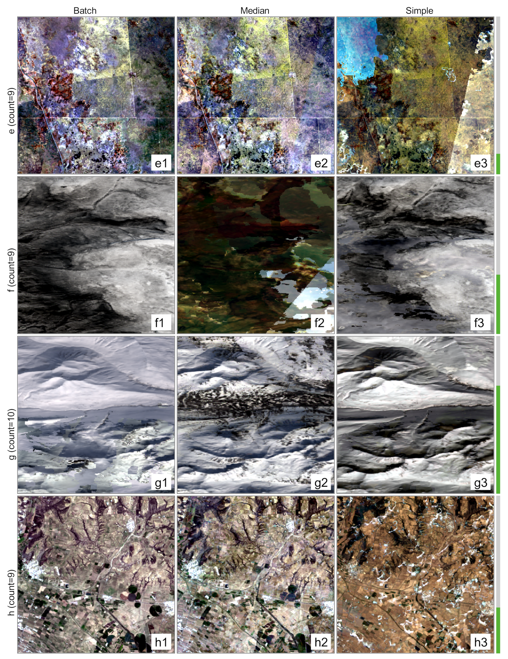
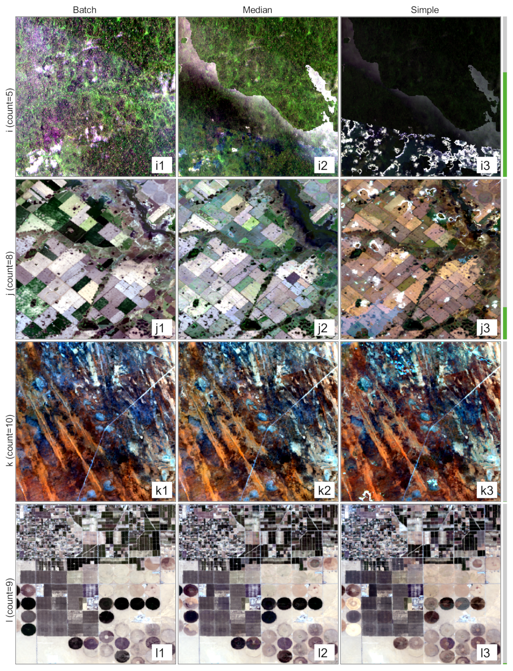
Figure 8, Figure 9 and Figure 10 show the band 4/3/2 compositing results of twelve locations obtained from the three algorithms, as well as the available image count and average cloud coverage at that location. The following comparison focuses on three different aspects.
First of all, in terms of cloud coverage, the difference between the three algorithms is relatively small for locations with extremely low cloud coverage, such as locations e, j, k, and l. The difference between algorithms is also small for locations with exceptionally heavy cloud coverage, which may be due to a lack of data sources, such as locations d and g. The batch algorithm performs noticeably better than other algorithms with a middling cloud cover, such as locations a, b, c, f, h, and i.
Secondly, from the perspective of geographical location, locations f and g are near the Arctic area, whereas locations d and i are close to the equatorial zone. It can be seen that the batch sometimes performs well (location f and i) and sometimes as bad as other algorithms (location d and g). It indicates that the influence of latitude on the compositing results is far less as compared to the influence of cloud coverage.
Thirdly, in terms of seasonal factors, j and k are in the southern hemisphere’s winter, whereas a, b, c, and l are in the northern hemisphere’s summer. It can be seen that the compositions in winter are clearer than in the summer. This requirement is encountered by all three methods. The most probable explanation for it might be that in the winter cloud cover is much higher than in the summer. Despite considerable cloud coverage in the summer, the batch method obtains better results than other algorithms for locations a, b, and c.
From the context of visual comparison, the compositing results of the batch method are the clearest and unclouded. The batch algorithm minimizes the impact of cloud coverage and cloud shadow. In contrast, the results of the median method are randomly contaminated by a small amount of cloud cover. Similarly, the results of the simple method are affected by a large amount of cloud cover.
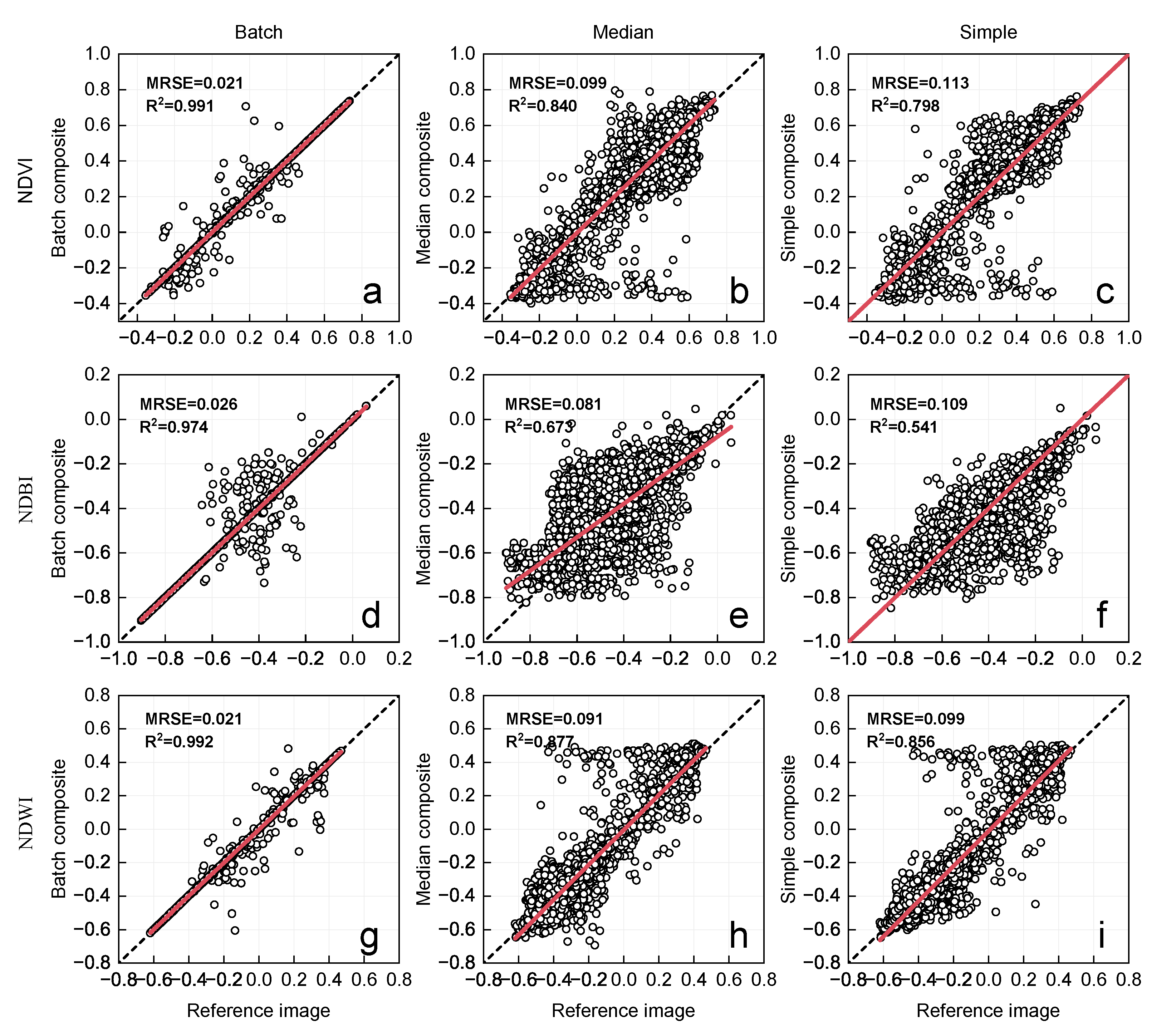
Band computations, such as NDVI, NDBI, and NDWI, were calculated from 5000 pixels, which were randomly selected from the visualization images as shown in Figure 11. The majority of the post-banding data of the batch algorithm were derived from the one-view image and a small amount of missing data were derived from the observations where the substitutes were located (Figure 11a,d,g). In contrast, the median (Figure 11b,e,h) and simple (Figure 11c,f,i) algorithms have scattered data sources and different bands from different observations, which brings uncertainty to the results of the band computation.
In comparison to the isolated pixel-based algorithm, two advances were obtained in this work based on the novel batch pixel-based algorithm. (1) The composite result shows a considerable reduction in pixel dispersion. (2) Band dispersion is no longer an issue.

4. Discussion

4.1. Principles of the Compositing Algorithms

In principle, isolated pixel-based algorithms are a group of algorithms that use a single pixel as the unit of computation to determine the best value for each pixel in each band using a statistical aggregation approach. For example, when the median algorithm calculates the B1 band, it first generates a set of B1 bands from all alternative images, and then generates a subset of all pixels at each position. Onward, the median or mean value of each subset is picked as the best value for that position. Furthermore, the simple algorithm appears similar to the median. The only difference between the two is that the median is replaced with the minimal value of the cloud possibility fraction. As a result, the isolated pixel-based algorithm’s primary criterion for pixel selection is numerical statistics. It does not distinguish the overall observation quality of the image and does not examine the relationship between pixels on the same image. This might lead to issues such as the unpredictability of pixel dispersion and band dispersion. The unpredictability of pixel dispersion in this context shows that distinct pixels are derived from separate observations in which dispersion seems unpredictable and increases quickly as the alternative set increases. The unpredictability of band dispersion exhibits that pixels in different bands are derived from different observations. For example, the red band may be derived from a bright April observation but the NIR band may be produced from a foggy June observation and the changing time and weather conditions may have unpredictable effects on the band computations.
The algorithm used in this study is different from the pixel-by-pixel selection described earlier, in which the best options are picked in batches rather than individually. In detail, it chooses the reference image that best meets the aim of the user’s research as the main portion of the result. Further, it selects the best substitute from the list of alternatives if the main portion is insufficient. Furthermore, a well-designed model (see Section 2.2.1) determines the priority of the alternatives automatically, taking into account of the observation quality, cloud cover, observation time, and sensor types of alternative images. As a result, the pixel dispersion is minimized because the reference image accounts for the majority of the final output, and the algorithm does not suffer from band dispersion because all bands of the alternative are processed as a whole.

4.2. Effects of Cloud Coverage, Latitude, and Season

The two primary factors affecting image compositing are “available observations count” and “cloud coverage”. The available count is determined by satellite parameters and observation conditions, which are directly affected by cloud coverage.
Latitude and season are two sub-factors that also make a difference. Seasonal variations frequently affect the available clouds and cloud coverage. For instance, in the northern hemisphere, the available count is substantially lower in the summer than in the winter due to the frequent surface atmospheric activity. The cloud coverage is significantly higher than it is in the summer. Furthermore, many remote sensing applications have specific limits for the season or observation period, which greatly affect the availability of remote sensing data.
From our statistics of all the scenes of Landsat 8 in 2019, the available counts in polar regions are significantly less than the lower altitude regions. The cloud coverage in equatorial regions and coastal regions is higher while in desert regions and inland regions it is relatively low.
On the other hand, in areas with extremely insufficient or excessive cloud coverage, there is basically little difference in the composite results; in other areas, the difference between the three algorithms is noticeably prominent. It should be emphasized that cloud cover continues to affect the compositing algorithms even after the cloud removal. It is possible that this is due to the cloud detection algorithm’s limitations for thin clouds, cloud shadows, etc. [38,39].

4.3. Significance of This Study

The algorithm in this study gives more reasonable results for the composite processing of multispectral optical satellite images and is especially valuable for the composite processing of long time-series images, which applies to Landsat series satellites, but can also be used with Sentinel-2, MODIS, and other sensors. It is especially suitable for remote sensing applications that require high compositing integrity, such as phenology [5], land use classification [13], and climate change [40] studies.
Moreover, the present algorithm is customizable and the parameter settings make it possible to meet the needs of various remote sensing applications. If the user is sensitive to the acquisition time, a relatively small number of observations can be used. If the user is sensitive to the integrity of the composition, a large enough observation frequency can be used to obtain higher compositing integrity.
The major contributions of this study are:
(1)
The paper proposes a new automated compositing algorithm for Landsat multi-temporal series images, which is implemented on the GEE cloud platform and is characterized by wide adaptability and high data concentration.
(2)
It suggests a method for quantifying composition assessment using temporal dispersion instead of human visual inspection and it solves several shortcomings and limitations of isolated pixel-based compositing algorithms.

4.4. Limitations and Potential Improvements

The compositing algorithm proposed in this study works well in most cases, but if the probability of local cloud coverage is too high in some extreme cases, it will lead to a small percentage of valid pixels in the reference image, resulting in a large percentage of missing pixels and a high degree of pixel dispersion in the compositing results. As a result, such compositing results may cast doubt on some specific analyses. The fundamental cause of this problem is the inadequate quality of the observations. In order to overcome it, the user may need to reduce the integrity of the composition to improve data concentration. In addition, to address this problem, extra observations might be combined from other similar satellites, such as Sentinel-2 and MODIS [41,42,43].
On the other hand, the algorithm in this study majorly depends on cloud and cloud shadow detections. It uses the Fmask [27,30] for cloud masking in the demonstration application mentioned in Section 2.2.6. In other words, it is the post-processing of the cloud-removal process. It follows that the compositing results of this algorithm, similar to other compositing algorithms, are limited by the influence of cloud and cloud shadow identification [35].

5. Conclusions

This study focuses on the compositing algorithm for optical satellite time-series images and proposes a batch pixel-based compositing algorithm for Landsat with the implementation and source code on the GEE platform. The algorithm uses all valid pixels from the reference image as the main part of the results, then selects substitutes in batch for the missing portions using a priority coefficient model. In the end, the main part and the missing parts are merged into the compositing result. Using all Landsat 8 observations from 2019, this study compares our algorithm and the isolated pixel-based algorithm provided by the GEE platform, highlighting solutions to the following problems: (1) Unpredictable pixel dispersion; (2) Unpredictable band dispersion; and (3) Reducing cloud and cloud shadow interference. Therefore, this algorithm has less bias, requires fewer observations, lowers pixel dispersion, and improves the future analysis of Landsat images. The approach provides a full and useful framework for the composition of long time-series images from Landsat series satellites with the potential to composite other optical satellite images.

Author Contributions

Conceptualization, J.M.; data curation, X.Y.; funding acquisition, J.M.; investigation, X.Y.; methodology, J.L.; project administration, J.M.; software, J.L.; validation, X.Y.; writing—original draft, J.L.; writing—review and editing, J.L. All authors have read and agreed to the published version of the manuscript.

Funding

This work was supported by a project by the Anhui Provincial Department of Education via grant KJ2018A0326.

Data Availability Statement

Data is contained within the article.

Acknowledgments

We thank the Google Earth Engine cloud platform for providing remote sensing data storage and analysis services, which played an important role in the smooth progress of our research.

Conflicts of Interest

The authors declare no conflict of interest.

Abbreviations

The following abbreviations are used in this manuscript:
GEEGoogle Earth Engine
DOYday of year
VIvegetation index
NIRnear-infrared
NDWInormal difference water index
NDBInormal difference built-up index

Appendix A

Table A1. List of sampling locations for visualization.
LocationLon.Lat.Path/RowMean Cloud
Cover (%)
Available
Image Count
a118.336713631.2981391120/3828.355
b121.688970931.3093027118/3858.536
c104.071256530.6049022129/3974.938
d24.47167350.0630941176/6069.557
e133.4560485−15.9006582104/7113.019
f107.440423565.3931218138/1437.659
g−152.715826562.297268472/1668.5910
h−97.872076519.370676825/4729.229
i−59.20020150.7661963231/5965.275
j−60.6064515−34.8341590226/8420.208
k21.6591735−28.2488155174/800.3010
l−114.607033032.551749238/370.809
Table A2. Compositing results of six integrity goals using three different algorithms.
Goals (%)MethodsObservation Number to Achieve the Integrity GoalTotal
1234567891011121314≥15
90.000Batch831180317731900000000009331
Median20537510041740191414759965433762261831039044579331
Simple460310656307517814913702211338066374223389331
95.000Batch7852983373803382000000009331
Median1742216319811589147014019065983882721891711032379331
Simple394312637195257206194763042401401026063371209331
99.000Batch439731481098371177712621114411019331
Median1582518420659284913061228114887866447035926110039331
Simple53926421542759546521562522410321230166120853669331
99.900Batch6812518208213709766683942251468250402617569331
Median158313643211163477506873900103186878461025689331
Simple1592857461308140810727485205314624303143012208279331
99.990Batch342152016161241996802683554364293193163123853569331
Median1580129141916032520453752480574487175040199331
Simple15511833756910151157109777863248349340341030013849331
99.999Batch1691009128410929078136605895194233222292021849299331
Median158012771823927311843832967253880367549729331
Simple15594190332663915104394688055451539445234318559331

References

  1. USGS. Landsat Missions. Available online: https://www.usgs.gov/landsat-missions/landsat-9 (accessed on 6 April 2022).
  2. Wulder, M.A.; Loveland, T.R.; Roy, D.P.; Crawford, C.J.; Masek, J.G.; Woodcock, C.E.; Allen, R.G.; Anderson, M.C.; Belward, A.S.; Cohen, W.B.; et al. Current status of Landsat program, science, and applications. Remote Sens. Environ. 2019, 225, 127–147. [Google Scholar] [CrossRef]
  3. Pontes-Lopes, A.; Dalagnol, R.; Dutra, A.C.; de Jesus Silva, C.V.; de Alencastro Graça, P.M.L.; de Oliveira e Cruz de Aragão, L.E. Quantifying post-fire changes in the aboveground biomass of an Amazonian forest based on field and remote sensing data. Remote Sens. 2022, 14, 1545. [Google Scholar] [CrossRef]
  4. Workie, T.G.; Debella, H.J. Climate change and its effects on vegetation phenology across ecoregions of Ethiopia. Glob. Ecol. Conserv. 2018, 13, e00366. [Google Scholar] [CrossRef]
  5. Younes, N.; Joyce, K.E.; Maier, S.W. All models of satellite-derived phenology are wrong, but some are useful: A case study from northern Australia. Int. J. Appl. Earth Obs. Geoinf. 2021, 97, 102285. [Google Scholar] [CrossRef]
  6. Grace, K.; Anderson, S.; Gonzales-chang, M.; Costanza, R.; Courville, S.; Dalgaard, T.; Dominati, E.; Kubiszewski, I.; Ogilvy, S.; Porfirio, L.; et al. A review of methods, data, and models to assess changes in the value of ecosystem services from land degradation and restoration. Ecol. Model. 2016, 319, 190–207. [Google Scholar] [CrossRef]
  7. Woodcock, C.E.; Allen, R.; Anderson, M.; Belward, A.; Bindschadler, R.; Cohen, W.; Gao, F.; Goward, S.N.; Helder, D.; Helmer, E.; et al. Free access to Landsat imagery. Science 2008, 320, 1011. [Google Scholar] [CrossRef]
  8. Zhu, Z. Change detection using landsat time series: A review of frequencies, preprocessing, algorithms, and applications. ISPRS J. Photogramm. Remote Sens. 2017, 130, 370–384. [Google Scholar] [CrossRef]
  9. Hemati, M.; Hasanlou, M.; Mahdianpari, M.; Mohammadimanesh, F. A systematic review of Landsat data for change detection applications: 50 years of monitoring the earth. Remote Sens. 2021, 13, 2869. [Google Scholar] [CrossRef]
  10. Hansen, M.C.; Loveland, T.R. A review of large area monitoring of land cover change using Landsat data. Remote Sens. Environ. 2012, 122, 66–74. [Google Scholar] [CrossRef]
  11. White, J.C.; Wulder, M.A.; Hobart, G.W.; Luther, J.E.; Hermosilla, T.; Griffiths, P.; Coops, N.C.; Hall, R.J.; Hostert, P.; Dyk, A.; et al. Pixel-based image compositing for large-area dense time series applications and science. Can. J. Remote Sens. 2014, 40, 192–212. [Google Scholar] [CrossRef] [Green Version]
  12. Masek, J.G.; Wulder, M.A.; Markham, B.; McCorkel, J.; Crawford, C.J.; Storey, J.; Jenstrom, D.T. Landsat 9: Empowering open science and applications through continuity. Remote Sens. Environ. 2020, 248, 111968. [Google Scholar] [CrossRef]
  13. Hansen, M.C.; Potapov, P.V.; Moore, R.; Hancher, M.; Turubanova, S.A.; Tyukavina, A.; Thau, D.; Stehman, S.V.; Goetz, S.J.; Loveland, T.R.; et al. High-resolution global maps of 21st-Century forest cover change. Science 2013, 342, 850–853. [Google Scholar] [CrossRef] [PubMed]
  14. Danylo, O.; Pirker, J.; Lemoine, G.; Ceccherini, G.; See, L.; McCallum, I.; Hadi; Kraxner, F.; Achard, F.; Fritz, S. A map of the extent and year of detection of oil palm plantations in Indonesia, Malaysia and Thailand. Sci. Data 2021, 8, 96. [Google Scholar] [CrossRef] [PubMed]
  15. Pekel, J.F.F.; Cottam, A.; Gorelick, N.; Belward, A.S. High-resolution mapping of global surface water and its long-term changes. Nature 2016, 540, 418–422. [Google Scholar] [CrossRef] [PubMed]
  16. Gong, P.; Liu, H.; Zhang, M.; Li, C.; Wang, J.; Huang, H.; Clinton, N.; Ji, L.; Li, W.; Bai, Y.; et al. Stable classification with limited sample: Transferring a 30-m resolution sample set collected in 2015 to mapping 10-m resolution global land cover in 2017. Sci. Bull. 2019, 64, 370–373. [Google Scholar] [CrossRef]
  17. Scheip, C.M.; Wegmann, K.W. HazMapper: A global open-source natural hazard mapping application in Google Earth Engine. Nat. Hazards Earth Syst. Sci. 2021, 21, 1495–1511. [Google Scholar] [CrossRef]
  18. Banerjee, A.; Chakrabarty, M.; Bandyopadhyay, G.; Roy, P.K.; Ray, S. Forecasting environmental factors and zooplankton of Bakreswar reservoir in India using time series model. Ecol. Inform. 2020, 60, 101157. [Google Scholar] [CrossRef]
  19. Wu, C.; Webb, J.A.; Stewardson, M.J. Modelling Impacts of Environmental Water on Vegetation of a Semi-Arid Floodplain–Lakes System Using 30-Year Landsat Data. Remote Sens. 2022, 14, 708. [Google Scholar] [CrossRef]
  20. Guindon, L.; Gauthier, S.; Manka, F.; Parisien, M.A.; Whitman, E.; Bernier, P.; Beaudoin, A.; Villemaire, P.; Skakun, R. Trends in wildfire burn severity across Canada, 1985 to 2015. Can. J. For. Res. 2021, 51, 1230–1244. [Google Scholar] [CrossRef]
  21. Holben, B.N. Characteristics of maximum-value composite images from temporal AVHRR data. Int. J. Remote Sens. 1986, 7, 1417–1434. [Google Scholar] [CrossRef]
  22. Luo, Y.; Trishchenko, A.; Khlopenkov, K. Developing clear-sky, cloud and cloud shadow mask for producing clear-sky composites at 250-meter spatial resolution for the seven MODIS land bands over Canada and North America. Remote Sens. Environ. 2008, 112, 4167–4185. [Google Scholar] [CrossRef]
  23. Roy, D.P.; Ju, J.; Lewis, P.; Schaaf, C.; Gao, F.; Hansen, M.; Lindquist, E. Multi-temporal MODIS–Landsat data fusion for relative radiometric normalization, gap filling, and prediction of Landsat data. Remote Sens. Environ. 2008, 112, 3112–3130. [Google Scholar] [CrossRef]
  24. Roy, D.P.; Ju, J.; Kline, K.; Scaramuzza, P.L.; Kovalskyy, V.; Hansen, M.; Loveland, T.R.; Vermote, E.; Zhang, C. Web-enabled Landsat Data (WELD): Landsat ETM+ composited mosaics of the conterminous United States. Remote Sens. Environ. 2010, 114, 35–49. [Google Scholar] [CrossRef]
  25. Potapov, P.; Turubanova, S.; Hansen, M.C. Regional-scale boreal forest cover and change mapping using Landsat data composites for European Russia. Remote Sens. Environ. 2011, 115, 548–561. [Google Scholar] [CrossRef]
  26. Griffiths, P.; van der Linden, S.; Kuemmerle, T.; Hostert, P. A pixel-based landsat compositing algorithm for large area land cover mapping. IEEE J. Sel. Top. Appl. Earth Obs. Remote Sens. 2013, 6, 2088–2101. [Google Scholar] [CrossRef]
  27. Zhu, Z.; Wang, S.; Woodcock, C.E. Improvement and expansion of the Fmask algorithm: Cloud, cloud shadow, and snow detection for Landsats 4–7, 8, and Sentinel 2 images. Remote Sens. Environ. 2015, 159, 269–277. [Google Scholar] [CrossRef]
  28. Google Earth Engine. API Reference. Available online: https://developers.google.com/earth-engine/apidocs (accessed on 2 June 2022).
  29. Zhao, C.; Wu, Z.; Qin, Q.; Ye, X. A framework of generating land surface reflectance of China early Landsat MSS images by visibility data and its evaluation. Remote Sens. 2022, 14, 1802. [Google Scholar] [CrossRef]
  30. Qiu, S.; Zhu, Z.; He, B. Fmask 4.0: Improved cloud and cloud shadow detection in Landsats 4–8 and Sentinel-2 imagery. Remote Sens. Environ. 2019, 231, 111205. [Google Scholar] [CrossRef]
  31. FAO. Methods & Standards. Available online: http://www.fao.org/ag/agn/nutrition/Indicatorsfiles/Agriculture.pdf (accessed on 20 December 2021).
  32. Van De Griend, A.A.; Owe, M. On the relationship between thermal emissivity and the normalized difference vegetation index for natural surfaces. Int. J. Remote Sens. 1993, 14, 1119–1131. [Google Scholar] [CrossRef]
  33. Zha, Y.; Gao, J.; Ni, S. Use of normalized difference built-up index in automatically mapping urban areas from TM imagery. Int. J. Remote Sens. 2003, 24, 583–594. [Google Scholar] [CrossRef]
  34. Goksel, C. Monitoring of a water basin area in Istanbul using remote sensing data. Water Sci. Technol. 1998, 38, 209–216. [Google Scholar] [CrossRef]
  35. Scaramuzza, P.L.; Bouchard, M.A.; Dwyer, J.L. Development of the landsat data continuity mission cloud-cover assessment algorithms. IEEE Trans. Geosci. Remote Sens. 2012, 50, 1140–1154. [Google Scholar] [CrossRef]
  36. Perin, V.; Tulbure, M.G.; Gaines, M.D.; Reba, M.L.; Yaeger, M.A. On-farm reservoir monitoring using Landsat inundation datasets. Agric. Water Manag. 2021, 246, 106694. [Google Scholar] [CrossRef]
  37. Sirin, A.; Medvedeva, M. Remote sensing mapping of peat-fire-burnt areas: Identification among other wildfires. Remote Sens. 2022, 14, 194. [Google Scholar] [CrossRef]
  38. Zhang, Q.; Yuan, Q.; Li, J.; Li, Z.; Shen, H.; Zhang, L. Thick cloud and cloud shadow removal in multitemporal imagery using progressively spatio-temporal patch group deep learning. ISPRS J. Photogramm. Remote Sens. 2020, 162, 148–160. [Google Scholar] [CrossRef]
  39. Candra, D.S.; Phinn, S.; Scarth, P. Cloud and cloud shadow masking for Sentinel-2 using multitemporal images in global area. Int. J. Remote Sens. 2020, 41, 2877–2904. [Google Scholar] [CrossRef]
  40. Hantson, S.; Huxman, T.E.; Kimball, S.; Randerson, J.T.; Goulden, M.L. Warming as a Driver of Vegetation Loss in the Sonoran Desert of California. J. Geophys. Res. Biogeosci. 2021, 126, e2020JG005942. [Google Scholar] [CrossRef]
  41. Chen, N.; Tsendbazar, N.E.; Hamunyela, E.; Verbesselt, J.; Herold, M. Sub-annual tropical forest disturbance monitoring using harmonized Landsat and Sentinel-2 data. Int. J. Appl. Earth Obs. Geoinf. 2021, 102, 102386. [Google Scholar] [CrossRef]
  42. Guan, X.; Huang, C.; Zhang, R. Integrating MODIS and Landsat data for land cover classification by multilevel decision rule. Land 2021, 10, 208. [Google Scholar] [CrossRef]
  43. Li, S.; Wang, J.; Li, D.; Ran, Z.; Yang, B. Evaluation of Landsat 8-like land surface temperature by fusing Landsat 8 and MODIS land surface temperature product. Processes 2021, 9, 2262. [Google Scholar] [CrossRef]
Figure 1. Availability of observation data from different Landsat satellites. The satellites marked in blue are still operational, and the ones marked in yellow are no longer available. An SLC-off failure occurred on Landsat 7 since 31 May 2003, which had a significant impact on data quality; with the launch of Landsat 9, its use in combination with Landsat 8 will increase the time resolution to a true 8-day period.
Remotesensing 14 04252 g001
Figure 2. Map of the test sample and visualization sample distribution. The test sample locations were uniformly spread throughout 9331 sites based on the available Landsat 8 observations in 2019. From May to September 2020, the 12 visual points (see Table A1) were restricted to the Landsat 8 observation site. They were chosen on the basis of cloud cover and geographical location.
Remotesensing 14 04252 g002
Figure 3. Flow chart of the algorithm. The blue section shows the calculation of the main part of the compositing result, the red section shows the method to compute the missing pixels except for the main part, and the yellow section describes the priority index model.
Remotesensing 14 04252 g003
Figure 4. Global spatial distributions of all available Landsat 8 scenes counts and the mean cloud cover in 2019. Among these, (a) represents the distribution of the number of available observations count, and (b,c) represent the mean available count of the longitude and latitude directions, respectively; (d) shows the distribution of cloud coverage, and (e,f) represent the average cloud cover of the longitude and latitude directions, respectively.
Remotesensing 14 04252 g004
Figure 5. Comparison of the success rates of the three compositing algorithms for the 9331 tiles with different PATHs/ROWs in 2019. There are separate integrity goals ranging from 90 % to 99.999 % for each of the six subplots (af).
Remotesensing 14 04252 g005
Figure 6. Spatial distribution of the required observation count for 99% integrity of the global composition in 2019; (a) shows the algorithm used in this study; (b,c) show the median and simple algorithms.
Remotesensing 14 04252 g006
Figure 7. (ac) Trend graph of the relationship between the required scenes count and cloud coverage in 2019. In the first 1–1 group, the cloud coverage of the images used by the batch method is the lowest. Comparatively, only the batch trend shows a considerable increase in the trend.
Remotesensing 14 04252 g007
Figure 8. Visual comparison part 1: Band 4/3/2 composition produced by different algorithms at locations from (ad). Each location discloses the number of available image scenes (count variable from the left edge) and the average cloud coverage. The latter is represented by the vertical progress bar (max is 100%) on the right edge; (a1,b1,c1,d1) are produced with the batch algorithm, (a2,b2,c2,d2) are produced with the median algorithm, and (a3,b3,c3,d3) are produced with the simple algorithm.
Remotesensing 14 04252 g008
Figure 9. Visual comparison part 2: band 4/3/2 composition produced using different algorithms at locations from (eh). Each location discloses the number of available image scenes (count variable from the left edge) and the average cloud coverage. The latter is represented by the vertical progress bar (max is 100%) on the right edge; (e1,f1,g1,h1) are produced with the batch algorithm, (e2,f2,g2,h2) are produced with the median algorithm, and (e3,f3,g3,h3) are produced with the simple algorithm.
Remotesensing 14 04252 g009
Figure 10. Visual comparison part 3: band 4/3/2 composition produced using different algorithms at locations from (il). Each location discloses the number of available image scenes (count variable from the left edge) and the average cloud coverage. The latter is represented by the vertical progress bar (max is 100%) on the right edge; (i1,j1,k1,l1) are produced with the batch algorithm, (i2,j2,k2,l2) are produced with the median algorithm, and (i3,j3,k3,l3) are produced with the simple algorithm.
Remotesensing 14 04252 g010
Figure 11. Scatterplot of the differences between NDVI (ac), NDBI (df), and NDWI (gi) for different algorithms.
Remotesensing 14 04252 g011
Table 1. Comparison of the compositing success rate with an observation time limit of 2 months.
MethodsIntegrity (%)
90.00095.00099.00099.90099.99099.999
Batch99.9%99.5%96.6%71.3%50.6%38.1%
Median35.6%21.5%6.1%3.6%3.2%3.1%
Simple75.5%69.1%58.8%26.8%12.6%8.3%
Publisher’s Note: MDPI stays neutral with regard to jurisdictional claims in published maps and institutional affiliations.