Article

H2A2Net: A Hybrid Convolution and Hybrid Resolution Network with Double Attention for Hyperspectral Image Classification

1
School of Computer Science and Engineering, Nanjing University of Science and Technology, Nanjing 210094, China
2
School of the Internet of Things, Nanjing University of Posts and Telecommunications, Nanjing 210003, China
*
Author to whom correspondence should be addressed.
Remote Sens. 2022, 14(17), 4235; https://doi.org/10.3390/rs14174235
Submission received: 11 July 2022 / Revised: 16 August 2022 / Accepted: 24 August 2022 / Published: 27 August 2022
(This article belongs to the Section Remote Sensing Image Processing)

Abstract

:
Deep learning (DL) has recently been a core ingredient in modern computer vision tasks, triggering a wave of revolutions in various fields. The hyperspectral image (HSI) classification task is no exception. A wide range of DL-based methods have shone brilliantly in HSI classification. However, understanding how to better exploit spectral and spatial information regarding HSI is still an open area of enquiry. In this article, we propose a hybrid convolution and hybrid resolution network with double attention for HSI classification. First, densely connected 3D convolutional layers are employed to extract preliminary spatial–spectral features. Second, these coarse features are fed to the hybrid resolution module, which mines the features at multiple scales to obtain high-level semantic information and low-level local information. Finally, we introduce a novel attention mechanism for further feature adjustment and refinement. Extensive experiments are conducted to evaluate our model in a holistic manner. Compared to several popular methods, our approach yields promising results for four datasets.

Graphical Abstract

1. Introduction

Hyperspectral images (HSIs), as a branch of remote sensing images, are enjoying considerable interest from researchers owing to the abundant spatial and spectral information embedded within them. Compared with panchromatic images and multispectral remote sensing images, HSIs make it possible to discriminate different targets within a scene more accurately on account of their hundreds of continuous and narrow spectral bands. As a result, HSIs are widely used in many fields, including food [1], agriculture [2], and geology [3].
To implement these applications, a number of tasks have been developed on the basis of HSIs, such as classification [4], anomaly detection [5], and image decomposition [6]. Among these tasks, HSI classification is a fundamental yet challenging problem. To yield superior performance, there are two characteristics of HSIs which need be fully considered by researchers: (1) the rich spectral information and (2) the strong spatial correlation between pixels. Both can be investigated separately and independently or can be considered for joint information extraction, leading to different lines of work, such as spectral classification and spectral–spatial classification [7].
In the early days, statistical learning and machine learning were dominant. A number of algorithms from these fields were introduced into HSI classification and generated decent performances. Typical examples include principal component analysis (PCA) [8], linear discriminant analysis (LDA) [9], and independent component analysis (ICA) [10]. Due to insufficient training samples, copious spectral information can be a mixed blessing when being imposed upon high-dimensional HSI data suffering from a curve of dimensionality (i.e., the Hughes phenomenon) [11,12]. The essence of these techniques in statistical learning is to transform the HSI spectral vector from high-dimensional feature space to a low-dimensional feature space, eliminating redundant information and mitigating interference with subsequent feature extractions. In addition to the above, algorithms in machine learning, such as multinomial logistic regression (MLR) [13], support vector machine (SVM) [14], decision trees [15], and random forests [16], also played an important role in HSI classification, serving feature extraction or directly as classifiers. However, only exploiting spectral information is of no concern for HSI classification. Extensive experiments have validated that it is beneficial to introduce prior information, such as adjacent pixels located in homogeneous regions, which may be of the same class. There is a consensus that combined spectral–spatial classification is superior to spectral classification, and numerous efforts have been made to probe this possibility. For example, patch-wise-feature-extraction methods were applied instead of pixel-wise feature-extraction approaches in [17], which allowed for not only the excavation of spectral information but also the exploration of relationships between pixels. Other than that, researchers proposed methods for joint spectral–spatial feature extraction based on spectral–spatial regularized local discriminant embedding [18] and tensor discriminative locality alignment [19]. Although these traditional methods meet with some success, they significantly hinge on the handcrafted features. Nevertheless, these features tend to frustrate the expectations of a comprehensive representation of the complex contents within HSIs, bringing the development of HSI classification to a bottleneck.
Recently, deep learning (DL) has been widely embraced by the computer vision community, demonstrating excellent performance in various tasks. The advantage of deep learning is the ability to automatically learn richer features than conventional handcrafted features. Consequently, DL-based methods have been gaining traction with researchers in HSI classification. A range of DL-based methods for HSI classification have been proposed, such as stacked autoencoders (SAEs) [20,21], deep belief networks (DBNs) [22,23] and convolution neural networks (CNNs) [24,25]. In particular, due to the inherent properties of local connectivity and weight sharing, CNNs show better potential. By stacking convolutional layers, CNNs can capture a rich range of features from low-level to high-level. In [26], 1D-CNN was applied for the first time to extract spectral features. Romero et al. [27] also made use of 1D-CNNs to process spectral information. To improve feature representation and incorporate spatial information, 2D-CNNs have also attracted much attention. Feng et al. [28] designed a 2D-CNN framework to fuse spectral–spatial features from multiple layers and enhance feature representation. Lee et al. [29] drew on the idea of residual networks [30] to build a deep network to extract richer spectral–spatial features. Also, some works [29,31] prefer the application of PCA to reduce the dimensionality of the HSI data and then adopt a 2D-CNN for feature extraction and classification. However, it is obvious that considering spatial and spectral information separately betrays the relationship between them. To combat this problem, a 3D-CNN, as a CNN structure that can jointly extract spectral–spatial information, has been widely deployed to maintain the inherent continuity of the 3D-HSI cube. For instance, in [32], Zhong et al. developed a HSI classification model equipped with a 3D-CNN and a residual network (SSRN), which was effective at limiting the training samples. Moreover, Roy et al. [33] proposed a hybrid CNN, comprising a spectral–spatial 3D-CNN and a spatial 2D-CNN. Wang et al. [34] designed their fast dense spectral–spatial convolution (FDSSC) network based on DenseNet [35]. Compared to 2D-CNNs, 3D-CNNs perform better but exacerbate the demand on computing.
Although there has been plenty of excellent DL-based work in HSI classification, refining the features and further improving the accuracy of recognition remains challenging. To this end, attention mechanisms are often deployed to optimize the extracted features. As means of re-measuring the importance of information, attention mechanisms can bias the allocation of available computational resources to those signals that contribute more to the task [36,37]. Attention mechanisms have demonstrated promising results for computer vision tasks, such as sequence learning [38], image caption [39], and scene segmentation [40]. Inspired by these successful efforts, researchers introduced the attention mechanism to HSI classification. Mei et al. [41] proposed a spectral–spatial attention network (SSAN). In addition, given that HSI data possess spectral and spatial information simultaneously, it is an intuitive idea to build two branches to extract the features separately and then fuse them before classification. In [42], a double-branch multi-attention mechanism network (DBMA) was proposed based on the convolutional block attention module (CBAM) [43]. Furthermore, Li et al. [44] designed a double-branch dual-attention mechanism network (DBDA) for HSI classification. Also, using a double-branch structure, Shi et al. [45] designed a subtle attention module and obtained desirable results. Although these networks can achieve promising results, their attention mechanisms are too simple to learn crucial features.
Different from those found in CNNs, the transformer is a completely self-attention-based architecture, which is adept at capturing long-range dependencies. This structure originated from NLP tasks, and Vision Transformer (ViT) [46] introduced this idea to computer vision tasks for the first time. Then, plenty of models based on the transformer architecture shone in different computer vision tasks. Some work has been carried out with efforts to apply the transformer architecture to HSI classification. Hong et al. [47] and He et al. [48] reconceptualized HSI data from a sequence-data perspective, which adopted group-wise spectral embedding and transformer encoder modules to model spectral representations. Sun et al. [49] developed a new model called spectral–spatial feature tokenization transformer (SSFTT), which can encode the spectral–spatial information into tokens and then process them with a transformer. Similarly, Qing et al. [50] designed a spectral attention process and incorporated it into the transformer, capturing the continuous spectral information in a decent manner. However, these improved transformer methods all treated a spectral band or a spatial patch as a token and encoded all tokens, resulting in significant redundant calculations since the HSI data already contained substantial redundant information. In addition, given the differences between natural images and HSIs, transferring and processing the transformer, regarding the conversion of natural images directly into HSI classification, may lead to misclassification, especially for boundary pixels across classes. Last but not least, the inherent drawbacks of the transformer architecture, such as the lack of obtaining local information, the difficulty in training, and the requirement of complex parameters tuning, also limit the performance of these models in HSI classification.
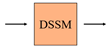
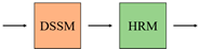
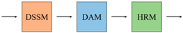
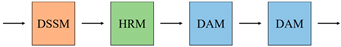
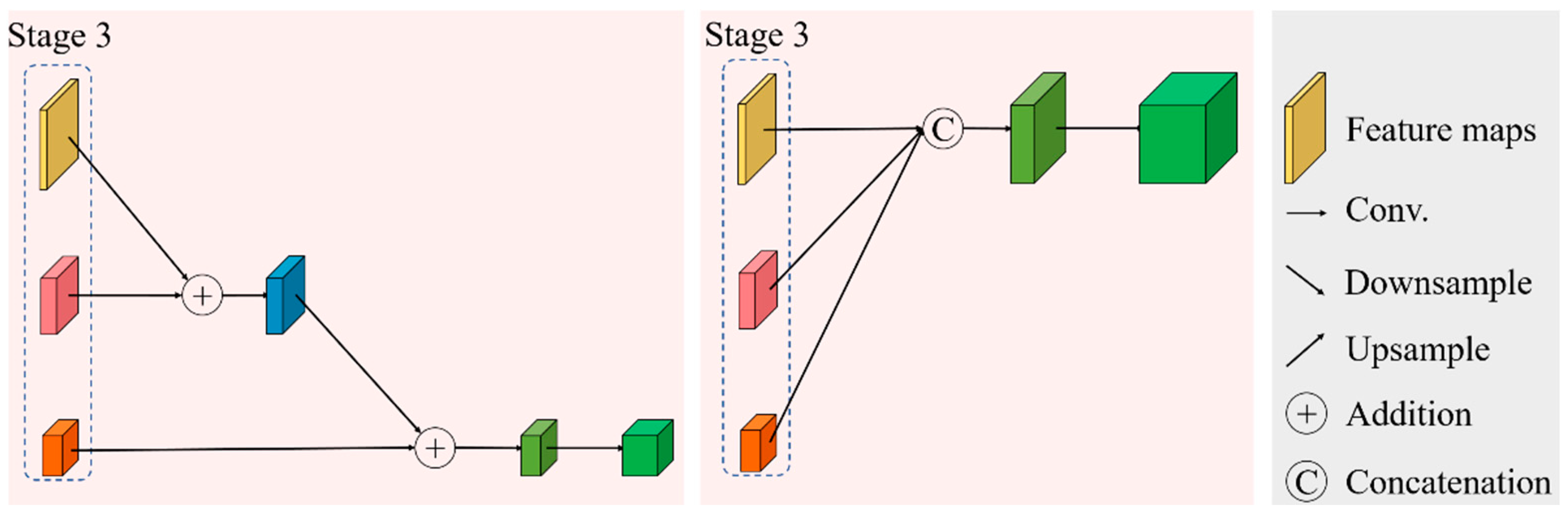
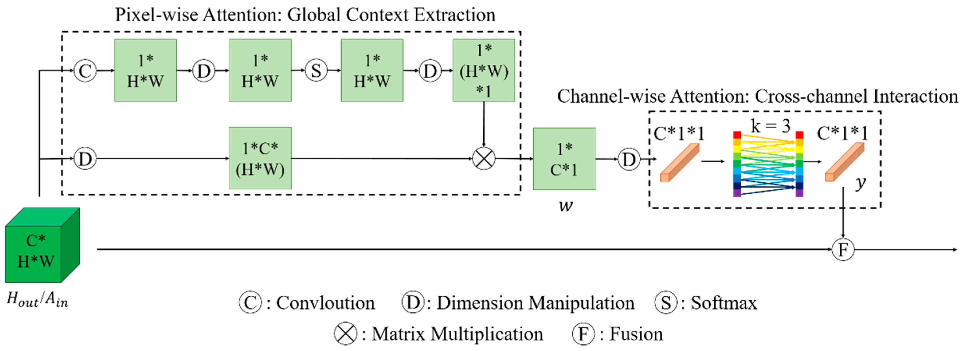
In this article, we propose a novel hybrid-convolution and hybrid-resolution network with double attention named H 2 A 2 Net. Hybrid convolution means that the 3D-convolution operators and 2D-convolution operators are jointly employed throughout the network to strike a better balance between speed and accuracy. Hybrid resolution means that the features are extracted at different scales. H2 refers to the above two aspects. Double attention means that two attention techniques are applied in combination, which is represented by A2. The H 2 A 2 Net mainly consists of three modules, namely a dense spectral–spatial module (DSSM), a hybrid resolution module (HRM), and a double attention module (DAM). The DSSM connects the 3D convolutional layers in the form of DenseNet to extract spectral–spatial features from the HSIs. HRM acquires strong semantic information and precise position information by parallelizing those branches with different resolutions, together with the constant interaction between different branches. The DAM is designed to implement two kinds of attention mechanisms in sequence, highlighting spatial and spectral information that is beneficial to the classification at a low computational cost. We investigate the appropriate solution for HSI classification by assembling these modules in different ways. The main contributions of this article can be summarized as follows.
(1)
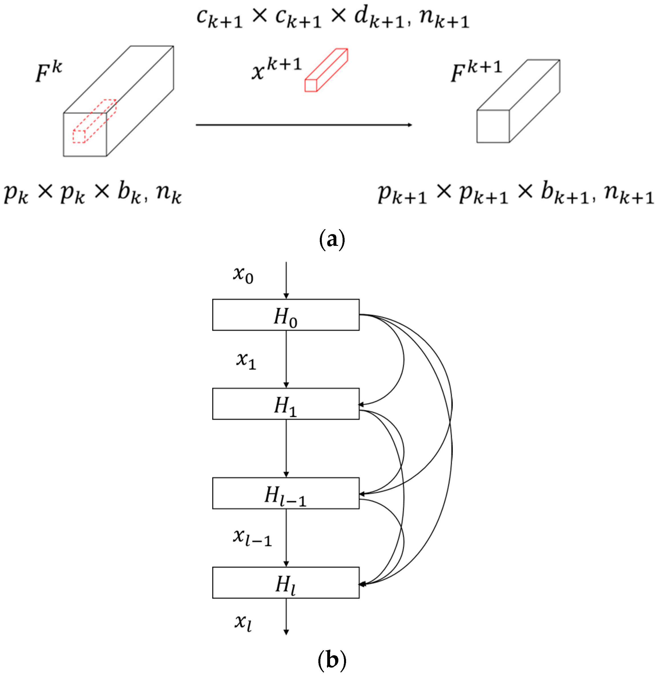
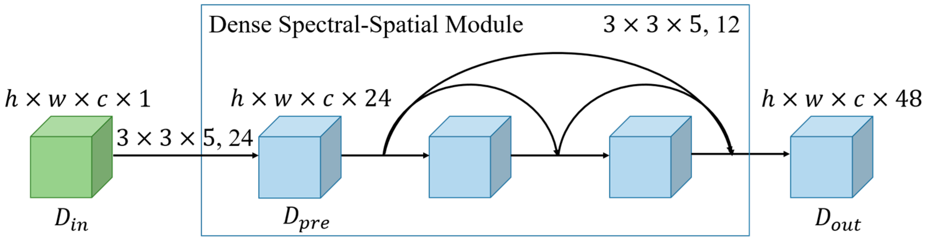
A densely connected module with 3D convolutions is integrated into a network, which aims to extract abundant spectral–spatial joint features by leveraging the inherent advantages of 3D convolution;
(2)
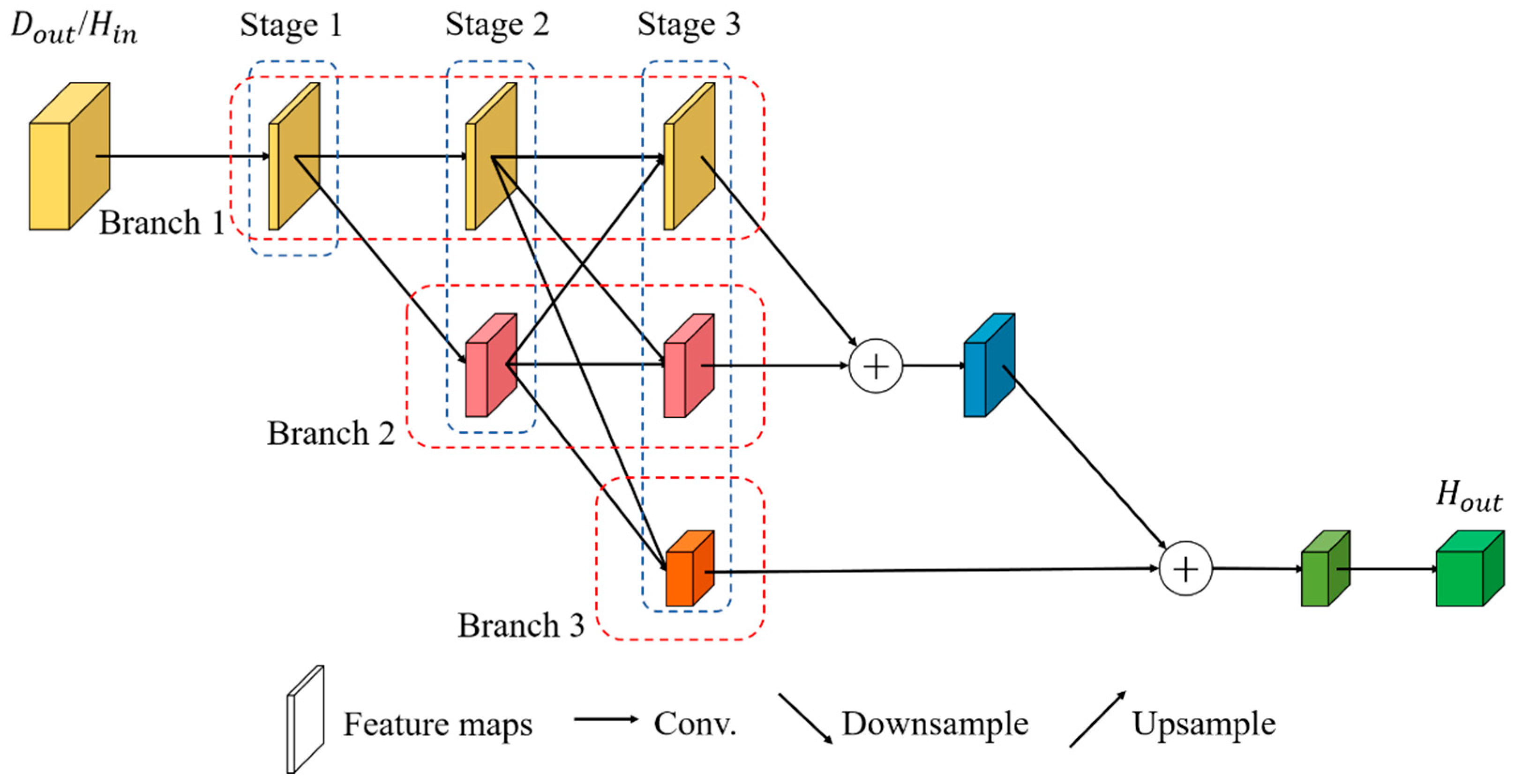
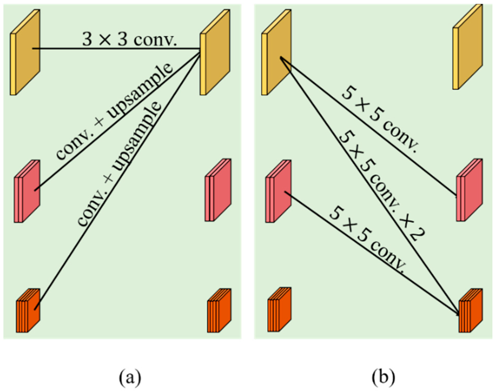
A hybrid resolution module is developed to learn how to extract multiscale spectral–spatial features from HSIs. Here, 2D convolutions are sufficient for our purposes. In addition, due to the cohabitation of high-resolution and low-resolution representations, it is possible for strong semantic information and precise position information to be learned simultaneously;
(3)
A novel double attention module is designed to capture interested spectral and spatial features, enhancing the informative features and suppressing the extraneous features.
(4)
Extensive experiments validate the performance of our approach, and the effects of the core ingredients are carefully analyzed.

2. Related Work

2.1. Low-Resolution, High-Resolution, and Hybrid-Resolution Representation Learning

Classical networks in deep learning, including AlexNet [51], VGGNet [52], and ResNet [30] share the same design philosophy: as the network goes deeper, the dimensionality of the feature maps increases, and the spatial size of the feature maps decreases. As a result, a low-resolution representation is obtained, which is subsequently processed before classification. Feature maps with a low resolution tend to contain stronger semantic information, yet this comes with a cost: the loss in resolution makes it difficult for the network to perform well within position-sensitive tasks.
For position-sensitive computer-vision tasks such as object detection, semantic segmentation, etc., high-resolution representation is necessary. To obtain high-resolution feature maps based on the CNN architecture, researchers have introduced up-sampling operations. Typical instances involve U-Net [53], Hourglass [54], and SegNet [55]. In addition, dilated convolution [56,57] and deconvolution [58] are common methods to upgrade the resolution. The former can reduce the number of down-sampling operations, while the latter can generate high-quality feature maps. In these networks, the ultimate high-resolution representation stems from two aspects: (1) the original high-resolution representation, which, when performing modest convolution operations, can only provide some low-level semantic information from the feature map, and (2) a high-resolution representation resulting from up-sampling a low-resolution representation. Although such a representation possesses abundant semantic information, the up-sampling process is unable to completely compensate for the loss in spatial resolution. The representation obtained by up-sampling is actually pseudo-high resolution since the practical contribution is largely limited by the low-resolution feature map with strong semantic information before up-sampling.
Breaking the stereotype of recovering high-resolution representations from low-resolution representations generated by CNNs, the High-Resolution Network (HRNet) [59,60] establishes a new paradigm for high-resolution representation learning. HRNet consistently maintains a high-resolution representation and gradually introduces low-resolution convolutions. By parallelizing branches with multiple resolutions and allowing constant interaction between branches, HRNet obtains strong semantic information and precise position information at the same time.

2.2. Attention Mechanisms

Attention mechanisms have been demonstrated as an effective methodology to fortify CNNs. Xu et al. first proposed a visual attention method for image-capture tasks. After that, many researchers began to pay attention to attentional mechanisms in computer vision. SENet [37] presented an efficacious attention mechanism to learn channel attention, pioneering this trend towards the study of channel attention mechanisms. In addition, GENet [61] helped to devise spatial attention to aggregate global contexts. Sharing the same philosophy, DAN [40], CBAM [43], and scSE [62] aimed to fuse spatial attention and channel attention in different ways. To model long-range dependency, NLNet [63] adopted a self-attention mechanism to generate pairwise relationships. Based on NL blocks, the creators of A2-Net [64] designed a novel relation function to assemble key features from spatial–temporal spaces into a single set and then adaptively assigned them to each pixel. These attention mechanisms can improve the quality of the extracted features and enhance the stability of the model, playing positive roles in the corresponding tasks.
In this paper, we introduce the attention mechanism to (1) capture long-range dependency in the spatial domain, complementing the local dependency modeling of CNNs, and (2) capture the cross-channel interaction from the spectral domain, obtaining complex channel dependency in an efficient manner.

3. Methodology

The flowchart of the proposed H 2 A 2 Net is illustrated in Figure 1. First, PCA is employed to reduce the dimensionality of the input 3D-HSI cube, aiming to obviate prohibitive memory and computational cost. In addition, using PCA can reduce redundant spectral information and speed up the training process. Note that there is no need to worry about information loss caused by PCA since many methods use PCA as one of the pre-processing steps and achieve satisfactory results, such as those with SSFTT. Second, the processed 3D cube is fed sequentially into the core ingredients of H 2 A 2 Net, including three modules: (1) a DSSM for feature extraction, which mimics the architecture of DenseNet with 3D convolution to extract the joint spectral–spatial features. (2) A HRM. Multiple branches with different resolutions in the module allow for precise spatial position information and strong semantic information at the same time. (3) A DAM, composed of pixel-wise attention and channel-wise attention. Pixel-wise attention serves for modeling the global context and capturing the long-range dependency between pixels, while channel-wise attention serves for cross-channel interaction. Finally, the output features are processed with global-average pooling, using a fully connected layer and a softmax classifier to obtain the classification results. Each element of the framework is described in detail in the following sections.

3.1. Dense Spectral–Spatial Module (DSSM)

With multiple convolution kernels, 2D convolution permits the simultaneous extraction of spectral and spatial information within HSIs yet lacks the ability to explore the consistency of diverse spectral bands. In contrast, 3D convolution can bridge this deficiency due to its inherent structure. Built upon this foundation, we implement a dense spectral–spatial module for preliminary spectral–spatial feature extraction by using DenseNet as a template.
A common 3D-convolutional layer is shown in Figure 2a. In detail, let the input HSI cube be Fk, which has a size of pk × pk × bk, nk. pk × pk, bk, and nk, which are the spatial size, depth dimensions, and input channels, respectively. Fk can be transformed to Fk+1 when convolved by a 3D-convolutional layer with a convolution kernel of size ck+1 × ck+1 × dk+1, nk+1. Usually, the batchnorm (BN) layer is appended to the convolutional layer to normalize the output for fast convergence. The complete procedure can be formulated as:
F i k+1 = σ ( j = 1 n k F ¯ j k x i k+1 + b i k+1 )
F ¯ k = F k E ( F k ) V a r ( F k )
where F j k p × p × b represents the j th input feature map of the ( k + 1 ) th layer. and σ ( . ) denotes the 3D convolution and the activation function. x i k + 1 and b i k + 1 represent the weights and biases of the i th filter in the ( k + 1 ) th layer. E ( . ) and V a r ( . ) denote the expectation and variance function, and F ¯ k is the product of the BN layer.
As for DenseNet, this is a classical network structure that connects all layers directly for feature reuse and enhanced feature propagation. Figure 2b demonstrates the structure of the basic unit of DenseNet. Accordingly, the input x l of l t h . layer can be formulated as:
x l = H l ( [ x 0 , x 1 , , x l 1 ] )
where H l refers to a module composed of convolution layers, activation layers, and BN layers, and [ x 0 , x 1 , , x l 1 ] denotes the concatenation of the feature maps generated by all preceding layers.
Since the 3D-convolution operation and DenseNet are now clearly elaborated, we can specify our dense spectral–spatial module, which is illustrated in Figure 3. Before feeding into the dense spectral–spatial module, the 3D cube is processed by PCA, and we denote the processed 3D cube as X h × w × c , where h , w , and c indicate the height, width, and the number of channels, respectively. To apply the 3D convolution, we need to transform X to D h × w × c × 1 . First, a 3D-convolutional layer with a 3 × 3 × 5 kernel size and 24 channels is applied to D , aiming to generate the preliminary input D p r e for the dense spectral–spatial module. As a result, the size of the resulting feature map D p r e is h × w × c × 24 . Then, the dense spectral–spatial module is attached. In this case, the 3D-convolutional layer with a 3 × 3 × 5 kernel size and 12 channels is employed twice. Finally, the output feature map D o u t with a size of h × w × c × 48 is obtained.

3.2. Hybrid Resolution Module (HRM)

The essence of the HSI classification task can be regarded as the classification of each pixel. Hence, this pixel-level problem requires a network with a strong position sensitivity. A natural thought is to exploit multi-scale features. Inspired by High Resolution Network (HRNet), we design the Hybrid Resolution Module (HRM) that allows for multi-resolution feature representations, which is illustrated in Figure 4. It is worth emphasizing that compared to HRNet, our HRM tailors to the characteristics of HSI by eliminating redundant feature extraction and attempting different feature fusion methods for multiple branches.
In order to be more parameter- and computation-conserving, we choose to rely on 2D convolution rather than 3D convolution in the module. To apply 2D convolution, D o u t h × w × c × f is reshaped to H i n R h × w × n , where n = c × f and f is 48 because of the number of 3D filters in the dense spectral–spatial module. Then, we address H i n with a 2D convolution layer to reduce the number of channels. By now, our preparations are complete, and we can commence building the module.
As is shown in Figure 4, the module contains three branches and three stages. The subnetwork starts with a high-resolution branch and gradually involves high-to-low resolution convolution streams. In each stage, a new branch is added in parallel with a larger number of channels and a smaller resolution. As a result, the more stages the subnetwork has, the more parallel branches with different resolutions there will be. In addition, the resolutions from the previous stages are retained in the later stages. Feature maps share an identical resolution and number of channels within the same branch. The resolution decreases and the number of channels increases from branch 1 to branch 3.
Apart from involving branches with different resolutions, it is important to exchange the information across multi-resolution representations. To this end, we developed a two-step criterion, i.e., alignment and fusion. In a nutshell, we up-sampled the low-resolution representation or used convolutions to down-sample the high-resolution representation before fusion. Specifically, a 3 × 3 convolution was adopted to bridge adjacent stages within the same branch. On the one hand, in the case of low-to-high resolution fusion, the representation from the low-resolution branch is convolved with a 1 × 1 convolution for aligning the number of channels, followed by the nearest up-sampling for aligning the resolution. Then, the transformed representation is added together with the target high-resolution representation to generate a new output. On the other hand, in the case of high-to-low resolution fusion, we down-sampled the input representation with convolutions. The kernel size of the convolution impacts the speed of resolution reduction. For a noticeable difference in resolution, we set the kernel size of the convolution to 5 × 5. The difference in resolution between branches determines the number of convolutions used. For example, one convolution is required between branch 1 and branch 2, while two convolutions are expected between branch 1 and branch 3. Using convolution for down-sampling ensures that the number of channels and resolution can be aligned simultaneously. Once the alignment is finished, we fuse the representations with an addition. The aforementioned procedure is depicted in Figure 5.
After multi-resolution fusion, we consider the construction of the output heads. Here, we attempt two schemes, as shown in Figure 6. One is to repeatedly down-sample and add to get the output. The other is to up-sample and concatenate. Both schemes are discussed in the experiments. In either case, a 1 × 1 convolution is attached at the end to raise the dimensionality of the feature map, which aims to enrich the information.

3.3. Double Attention Module (DAM)

HSI data contain rich information due to their inherent structure, which also means that there is colossal data redundancy. Hence, although the preceding modules can capture abundant spectral–spatial features, it is necessary to further accentuate the discriminative information and inhibit interference. To this end, the attention mechanism is adopted as our trump card. Following a simple design pattern, we design the DAM, which is shown in Figure 7.
Specifically, we implement the attention mechanism via a two-step strategy, which consists of pixel-wise attention and channel-wise attention. Pixel-wise attention aggregates the features of all positions to obtain global contextual features via a 1 × 1 convolution and a softmax function. Let x = { x i } i = 1 N be the input feature map, where N = H × W is the number of pixels and i denotes the index of position in the feature map. We compute a global attention map and assign it to all positions, which is expressed as:
w = j = 1 N e W k x j m = 1 N e W k x m x j
where W k denotes 1 × 1 convolution, e W k x j m = 1 N e W k x m represents the weight for global attention pooling. w is the intermediate feature map with the global context features.
When aggregating global contexts, we generally retain intact channels. After pixel-wise attention, we use channel-wise attention for cross-channel interaction. To capture the interaction between channels, an intuitive idea is to adopt a fully connected layer. However, it could result in a quadratic increase in the computational burden regarding the number of channels. To efficiently exploit channel information, we settled on extracting local cross-channel interactions. An empirical diagnosis of the coverage k of the interaction will be performed in the following section to strike a balance between efficiency and accuracy. In summary, channel-wise attention can be formulated as:
y = σ ( φ k ( w ) )
where φ k is a function that acts for channels within the coverage k and σ is an activation function.
The obtained y with double attention remains to be fused with the original input of the module, which aims to distribute the learned attention to each location. We denote the fusion function as F , then the fusion can be expressed as:
z i = F ( x i , y )
where z i represents the features at position i and there are two options for F , addition or multiplication.

4. Experiment

4.1. Datasets Description

To evaluate the proposed method, we carried out experiments on four well-known HSI datasets: the University of Pavia (UP), Salinas Valley (SV), Houston 2013 (HOU), and Kennedy Space Center (KSC) datasets.
The University of Pavia dataset was acquired by the reflective optics imaging spectrometer (ROSIS-3) sensor at the University of Pavia, northern Italy, 2001. After eliminating 12 noisy bands, it consists of 103 bands with a spatial resolution of 1.3 m per pixel in the wavelength range of 430 to 860 nm. The spatial size of the University of Pavia is 610 × 340 pixels, and 9 land cover classes are contained.
The Salinas Valley dataset was captured by the AVIRIS sensor over the agricultural area described as Salinas Valley in California, CA, USA, 1998. It comprises 204 bands with a spatial resolution of 3.7 m per pixel in the wavelength range of 400 to 2500 nm. The spatial size of the Salinas dataset is 512 × 217 pixels, and 16 land cover classes are involved.
The Houston 2013 dataset was provided by the Hyperspectral Image Analysis Group and the NSF-funded Airborne Laser Mapping Center (NCALM) at the University of Houston, US. It was originally adopted for scientific purposes in the 2013 IEEE GRSS Data Fusion Competition. The Houston 2013 dataset includes 144 spectral bands with a spatial resolution of 2.5 m in the wavelength range of 0.38 to 1.05 µm. The spatial size is 349 × 1905 pixels, and 15 land cover classes are involved.
The Kennedy Space Center dataset was captured by the AVIRIS sensor over the Kennedy Space Center, Florida, on 23 March 1996. It contains 224 bands, 10 nm in width, with a wavelength range of 400 to 2500 nm. After removing the water absorption and low SNR bands, 176 bands were conserved for the analysis. The spatial size of the Kennedy Space Center dataset is 512 × 614 pixels, and 13 land cover classes are contained.
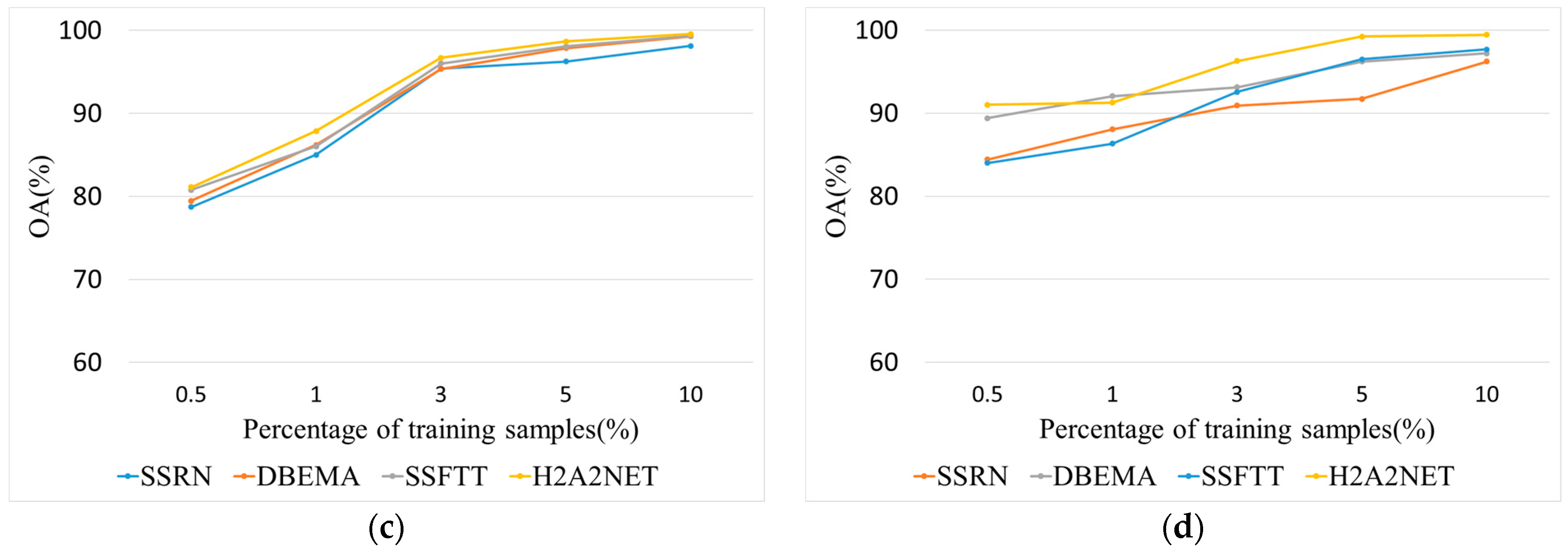
Depending on the size and complexity of the four datasets, we were able to set different sizes of training samples and validation samples to challenge all models. For UP and SV, we only selected 0.5% samples for training, 0.5% samples for validation, and 99% samples for testing. For KSC and HOU, we selected 3% samples for training, 3% samples for validation, and 94% samples for testing. Detailed figures of each category for training, validation, and testing sets are summarized in Table 1, Table 2, Table 3 and Table 4.

4.2. Experimental Configuration

To evaluate the performance of our model, three criteria were considered: overall accuracy (OA), average accuracy (AA), and kappa coefficient (K). All experiments were conducted on the platform configured with an Intel Core i7-8700K processor at 3.70 GHz, 32 GB of memory, and an NVIDIA GeForce GTX 1080Ti GPU. The software environment was the Windows 10 (64-bit) system for home and deep-learning frameworks of PyTorch.
In order to fully unleash the potential of H 2 A 2 Net, an advanced training recipe was used to train the model. The early stopping technique, regularization, and an advanced activation function were introduced to prevent overfitting. Concretely, we choose the Adam optimizer to train the network for 200 epochs under the guidance of the early stopping technique, i.e., the training process was terminated when the loss function no longer decreases within 10 epochs. The learning rate and the batch size were specified as 0.0001 and 64, respectively. In addition, a dropout layer with a 0.5 dropout rate was applied within the training protocol. Mish [65], as an advanced activation function, was adopted in lieu of ReLU, which is a common choice. The experiments were repeated 10 times, and the classification results for each category are now presented. Our preprocessing was to crop the raw HSI data into 3D cubes and then apply PCA. The number of spectral bands after PCA was set to 30.
Several models have been picked for our comparison. Following the identical recipes, we re-implemented these methods using their open-source code. The parameters were set in accordance with the corresponding article, and the input patch sizes for each model were specified according to the original article. The brief explanations and configurations of them are listed as follows:
(1)
SVM: each pixel, as well as all the spectral bands, was processed directly by the SVM classifier;
(2)
CDCNN: the structure of the CDCNN is illustrated in [29], which combines a 2D-CNN and ResNet. The input patch size is set to 5 × 5 × b, where b represents the number of spectral bands;
(3)
SSRN: the structure of the SSRN is illustrated in [32], which combines a 3D-CNN and ResNet. The input patch size is set to 7 × 7 × b;
(4)
DBDA: the structure of the DBDA is illustrated in [44], which is a double-branch structure based on a 3D-CNN, DenseNet, and an attention mechanism. The input patch size is set to 9 × 9 × b;
(5)
DBEMA: the structure of the DBEMA is illustrated in [45], which uses the pyramidal convolution and an iterative-attention mechanism. The input patch size is set to 9 × 9 × b;
(6)
ViT: the structure of the ViT is illustrated in [46], i.e., only including transformer encoders. Instead of patch-wise HSI classification, ViT processes the pixel-wise input in the HSI classification;
(7)
SSFTT: the structure of the SSFTT is illustrated in [49], which shows the design of a spectral–spatial feature tokenization transformer. The input patch size is set to 13 × 13 × b.

4.3. Classification Results

4.3.1. Analysis of the Up Dataset

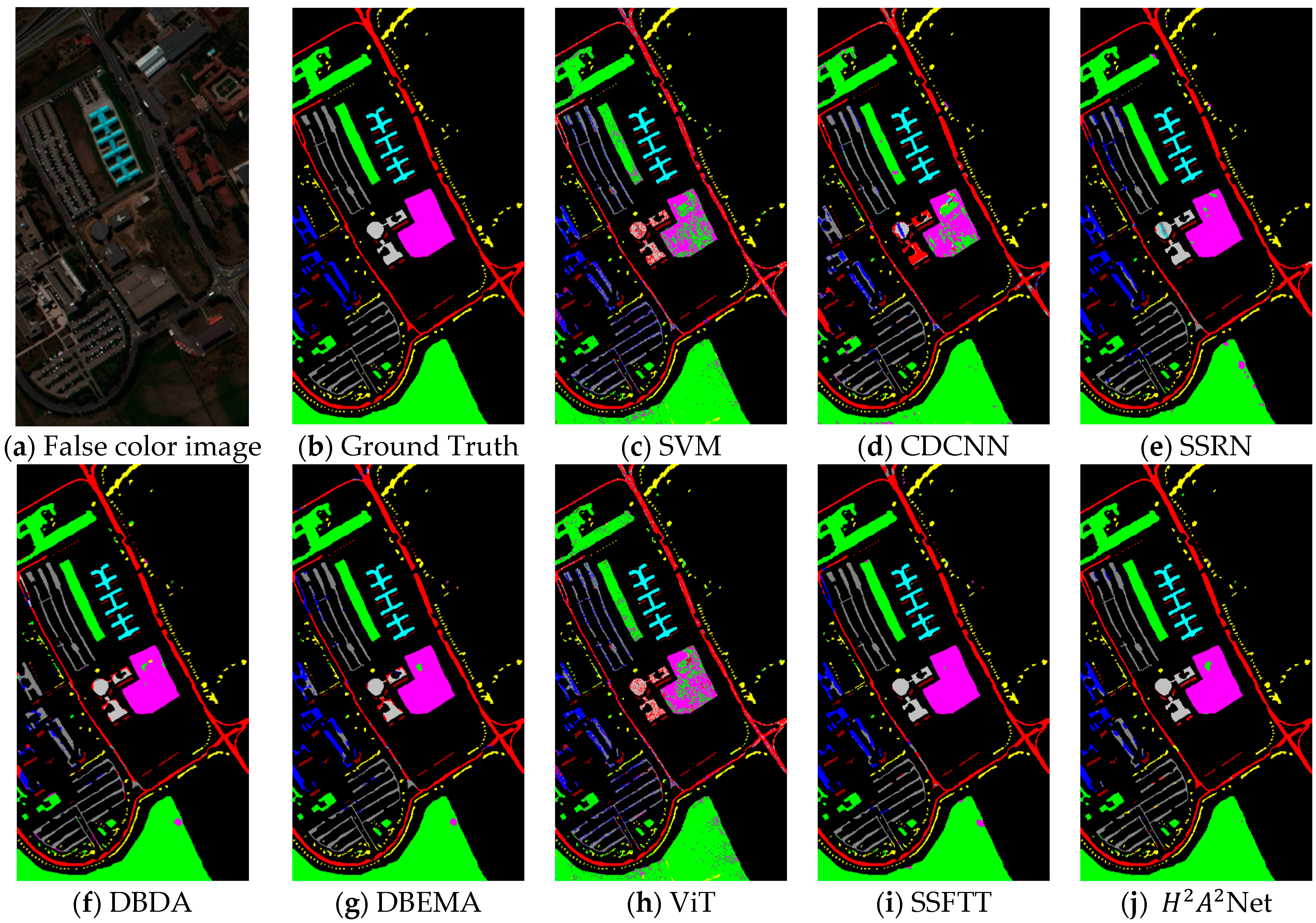
The classification results acquired via the different methods used on the UP dataset are presented in Table 5. Moreover, the corresponding classification maps of the different methods are shown in Figure 8. It can be noted from Figure 8 that the classification map generated by our H 2 A 2 Net is clearer than that obtained by any other method. Not only is the intra-class classification error small, but also the inter-class boundaries are clearly delineated. As indicated in Table 5, the proposed model delivers the best performance in terms of numerical results. In contrast to other methods, H 2 A 2 Net affords a 13.54% (SVM), 10.39% (CDCNN), 4.9% (SSRN), 4.08% (DBDA), 1.66% (DBEMA), 13.69% (ViT), 1.08% (SSFTT) accuracy increase over OA, respectively. Such excellent performance demonstrates that our model adequately captures and exploits spatial information as well as spectral information.
From the results, we can see that SVM, CDNN, and ViT had underperformed. The poor performance of SVM is understandable since it is a traditional method. CDCNN performs poorly because 2D-CNNs ignore the 3D nature of HSI data, and the training samples are insufficient. ViT does not work well due to its simple transformer structure and insufficient training samples. Other methods show decent performance as they are well designed, though there is still a gap between the performance of these and our H 2 A 2 Net. In addition, if we scrutinize the classification results for each category, it is noticeable that the proposed model is the only one that reaches above 90% accuracy for each category. In particular, for category 8, our model is the only method that achieves 90%+ accuracy. These observations demonstrate the stability and robustness of H 2 A 2 Net. Overall, our H 2 A 2 Net can consistently deliver superior performance on the UP dataset.

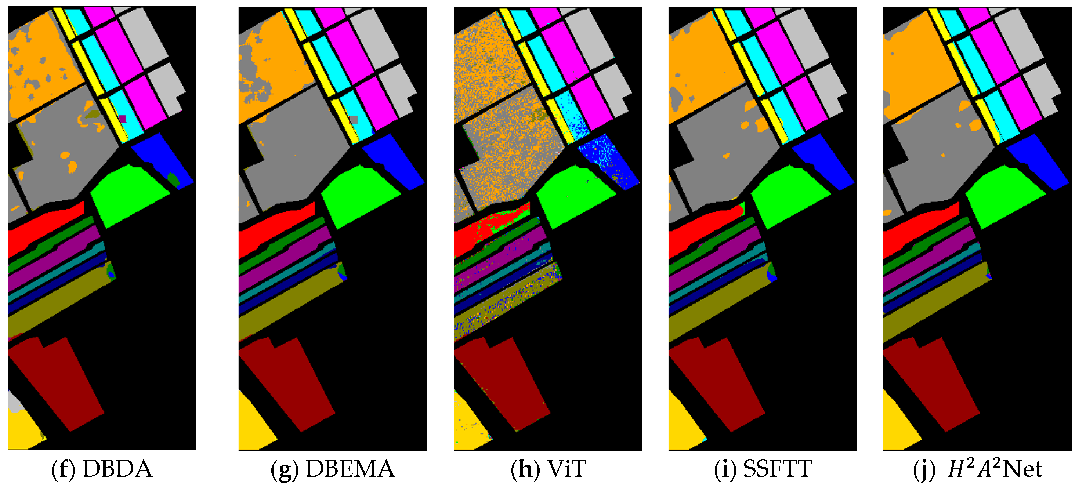
4.3.2. Analysis of the SV Dataset

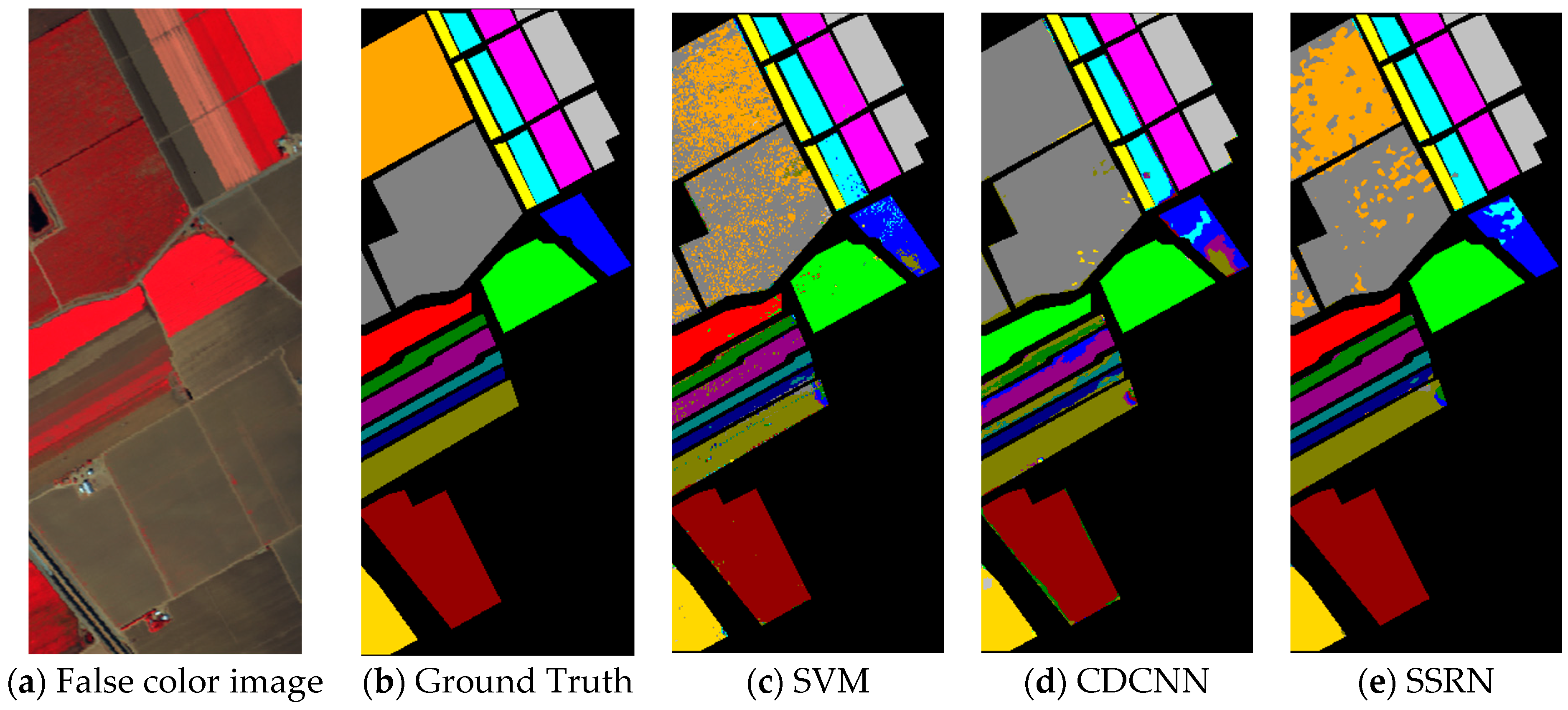
The classification results acquired via the different methods used on the SV dataset are presented in Table 6. Moreover, the corresponding classification maps for the different methods are shown in Figure 9. As illustrated in Figure 9, the classification map produced by our method is closest to the ground truth. Such positive results are also reflected in Table 6. As a comparison, H 2 A 2 Net has a 10.56% (SVM), 20.12% (CDCNN), 3.7% (SSRN), 3.61% (DBDA), 2.3% (DBEMA), 13.68% (ViT), 1.11% (SSFTT) accuracy increase over OA, respectively. These accuracy improvements suggest that our model can extract better features for classification.
SVM, CDCNN, and ViT still perform poorly. It can be concluded that the limited training samples are a huge limitation for them, especially for the latter two. Moreover, the other models still fail to compete with H 2 A 2 Net. For some categories in the SV dataset, e.g., categories 1, 2, 4, 6, 7, 9, 13, and 16, H 2 A 2 Net achieves 100% accuracy, which is greater than all models in terms of the number of categories that are perfectly classified. For the remaining categories, the results obtained by our model are also placed in the first echelon of all the models.

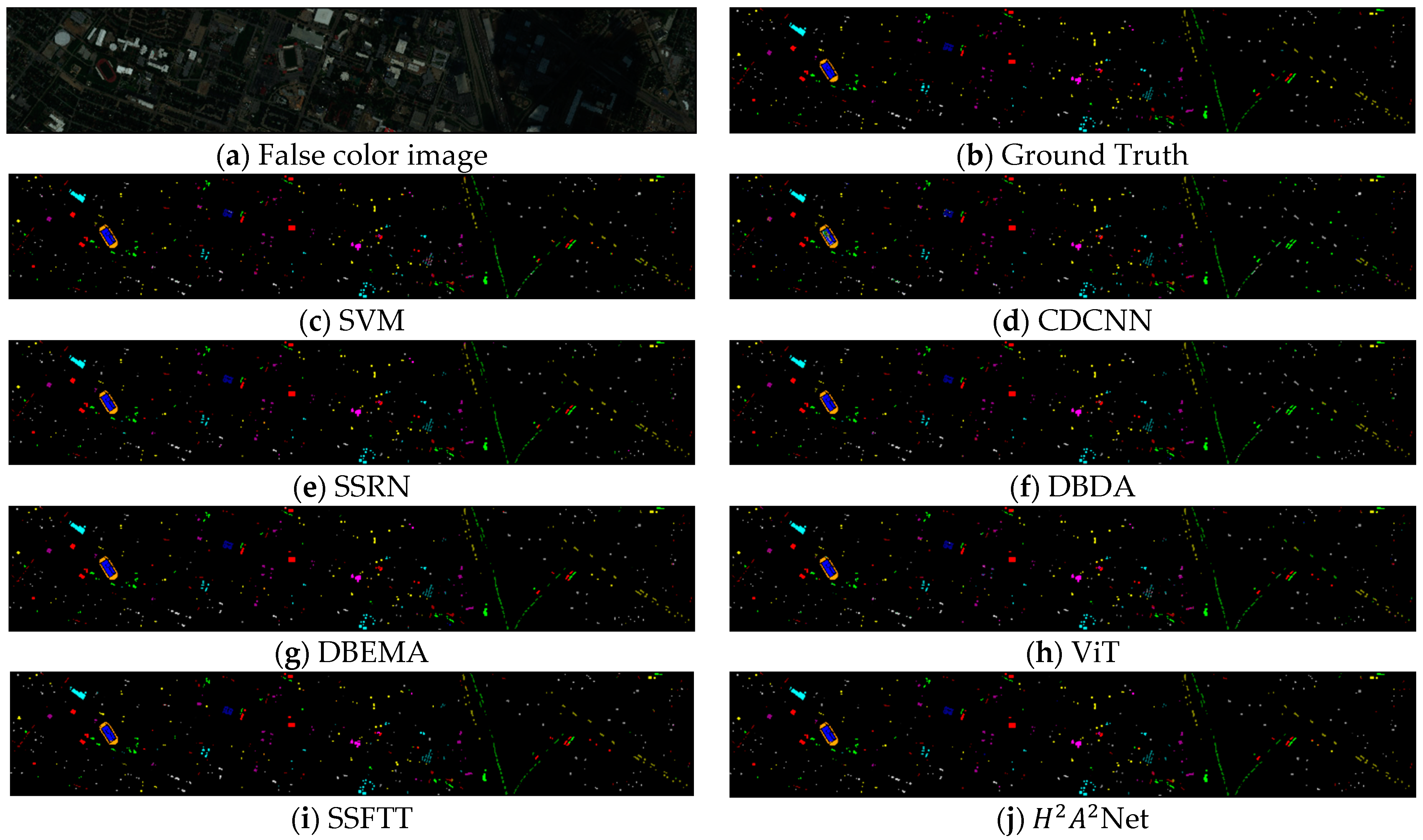
4.3.3. Analysis of the HOU Dataset

The classification results acquired via different methods for the HOU dataset are presented in Table 7. Moreover, the corresponding classification maps for the different methods are shown in Figure 10. The specific values of OA, AA, and Kappa are reported in Table 7. Compared with other methods, the increases of OA obtained by H 2 A 2 Net are 9.11% (SVM), 13.04% (CDCNN), 1.3% (SSRN), 3.87% (DBDA), 1.34% (DBEMA), 9.24% (ViT), and 1.65% (SSFTT).
Note that our model achieves the best performance in most of the categories of classification, including several 100% classification results. Due to the small size of the labeled samples and the large size of the HOU dataset, the distribution of the samples is scattered, implying that there are a large number of interfering pixels around the target pixel. Consequently, a side effect is imposed on the classification of certain categories. Nevertheless, since our model is equipped with a module for extracting features at multiple scales and a module for refining features with an attention mechanism, such challenges can be easily addressed. For example, for category 13, the best performance among all compared methods is 96.84% (SSRN), which is surpassed by 99.76% (our model).

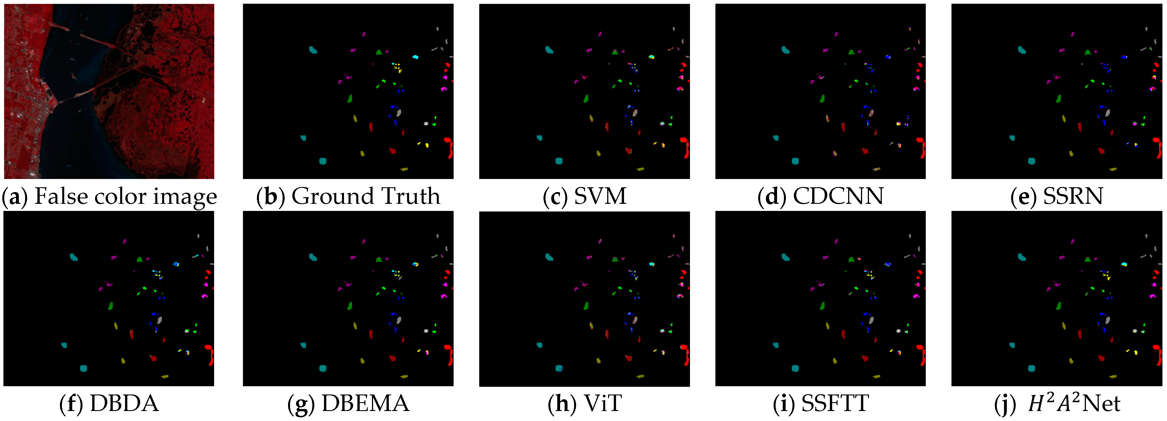
4.3.4. Analysis of the KSC Dataset

The classification results acquired via different methods for the KSC dataset are presented in Table 8. Moreover, the corresponding classification maps for the different methods are shown in Figure 11. As shown in Figure 11, the classification map obtained by H 2 A 2 Net is still the most similar to Ground Truth. Compared with the other methods, the increases obtained by H 2 A 2 Net for OA are 12.18% (SVM), 19.38% (CDCNN), 8.16% (SSRN), 5.98% (DBDA), 1.83% (DBEMA), 15.1% (ViT), and 3.73% (SSFTT). For each comparison, our model provides a significant gain of 1.5%, demonstrating that H 2 A 2 Net is adaptable to the KSC dataset.
Within six categories, our model achieved 100% accuracy. In this respect, our model stands out among all methods. For some categories, such as categories 3, 4, 5, and 6, it can be seen that all comparisons are unsatisfactory, except for our model. Using category 5 as an example, the best performance from all of the compared methods is 68.65% (DBEMA), which is inferior to the accuracy (97.91%) achieved by our model. Unfortunately, in category 7, our model did not perform well. However, this does not conceal the overall competence of H 2 A 2 Net. In general, our model shows convincing performances on the KSC dataset, overall, and individually.
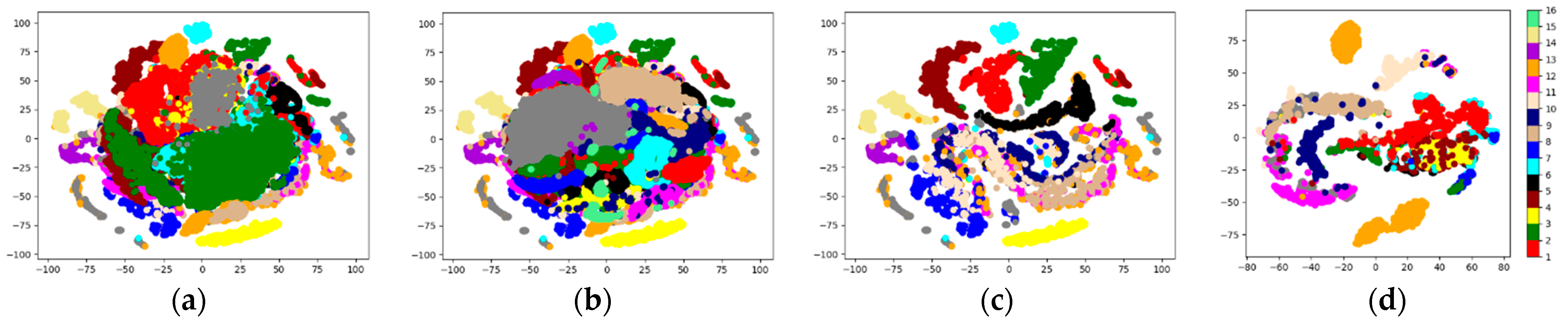
4.3.5. Visualization of H 2 A 2 Net Features

Figure 12 visualizes the original features and H 2 A 2 Net features for the four datasets. As can be observed from Figure 12a–d, plenty of the points in the original feature space are mixed up, posing difficulties to their classification. In contrast, from Figure 12e–h, it can be concluded that the data points in the transformed features space exhibit improved discriminability, demonstrating the ability of our network. In addition, points with the same color get closer once transformed, forming several clear clusters. In other words, H 2 A 2 Net can reduce the intra-class variances and increase the inter-class variances for HSI data, which is beneficial for classification.

5. Discussion

In this part, more experiments are discussed to comprehensively analyze the capabilities of our model.

5.1. Impact of the Proportion of Training Samples

For HSI classification, the performance of a model with a limited number of training samples is an important evaluation criterion. Therefore, we designed experiments to investigate the effect of different numbers of training samples on the model. For different datasets, we randomly selected 0.5%, 1%, 3%, 5%, and 10% of the samples to train our H 2 A 2 Net. The remaining samples were used to test H 2 A 2 Net. In addition, we choose three models as representatives of different types of networks for reference. The results are displayed in Figure 13. From Figure 13, we can conclude several points. First, the networks using 3D convolutions achieve decent results even if only 0.5% of the samples are used for training. Second, an increase in the proportion of training samples basically leads to an improvement in the performance of all four models. Third, H 2 A 2 Net outperforms other networks in most cases. Especially in the case of using fewer samples, such as only using 0.5% of the training samples on four datasets, where H 2 A 2 Net achieved the best performance. The above observations confirm the remarkable robustness and generalization of our model.

5.2. Parameter Analysis

As mentioned in Section 3.2, HRM down-samples the representation streams with different patch sizes while maintaining the original input image patch size. Thus, there are feature maps with different patch sizes in HRM. To explore the effect of the patch size on the model, we adopted image patches with different sizes as the original input, ranging from 13 to 21. Since we choose the HRM with three branches, the feature maps were down-sampled twice to obtain information at different scales. Furthermore, in order to guarantee the differentiation of representations within HRM, the patch size was designed to decrease using intervals of 4. Thus, five combinations of patch sizes were used to experiment with, i.e., 13-9-5, 15-11-7, 17-13-9, 19-15-11, and 21-17-13, which are denoted as 13, 15, 17, 19, and 21 in Figure 14, respectively. In addition, the value of k is also an important parameter within the DAM, which determines the scope of cross-channel interaction. Here, we analyze the effect of these parameters on the model. During parameter testing, other parameters, such as batch size and learning rate, were configured as described in the previous section.
Figure 14 illustrates the impact of the mutual effect of the patch size and the value of k on OA for the four datasets. It can be seen from Figure 14 that the patch size and the value of k affect OA, and the relationship between them cannot be easily represented by a convex function. However, Figure 14 shows that setting a suitable patch size and k value can obtain a promising result.

5.3. Ablation Study of Proposed Modules

To investigate the effect of these proposed modules and explore their proper connection styles, we designed six connection styles. Table 9 presents these ablation studies. The DSSM is always retained as the elementary component for extracting the features, and we gradually added other modules on top of it.
To make comparisons convenient, we adopt the smallest patch size combination, i.e., 13-9-5, here and in the following experiments. First, taking UP as an example, the OA of Style 1 is 81.14%, which is a poor performance. This indicates that simply using 3D convolutions is inadequate for HSI classification. Second, by comparing the results of Style 1, Style 2, and Style 3, it can be concluded that adding only the DAM makes the model weaker while adding only HRM can benefit the model. It might suggest that HRM can further enhance features to lift the model’s performance, while the DAM is unable to tune and improve the rudimentary extracted features. Third, by considering the results of Style 2, Style 3, Style 4, and Style 5, it is evident that a network with three modules outperforms a network with two modules. Furthermore, the results of Style 4 and Style 5 remind us that the order of the HRM and DAM matters. It is preferable to employ the DAM after the HRM. The reason is that the DAM requires abundant features to reach its full potential. Last but not least, the result of Style 6 shows that using more DAMs is a terrible idea. It can be observed from Table 9 that Style 5 already performs well. Adding another DAM leads to an increase in the complexity of the model, which may result in overfitting and thus make the model ineffective. The above discussions prove the rationality of our H 2 A 2 Net (which is Style 5) and reflects the fact that each module can contribute to the HSI classification to some extent.

5.4. Analysis of Submodel

5.4.1. Analysis of the HRM

In this section, we study the design elements of the HRM. As mentioned in Section 3.2, two elements are ablated, which are the number of branches and output heads. First, based on H 2 A 2 Net, we fixed the settings of the DSSM and DAM and only varied the number of branches in the HRM. We tagged H 2 A 2 Net with the number of branches. For example, “B2” means that the HRM in the model has two branches. Figure 15 presents the OA scores of these models for the four datasets. The results demonstrate that the choice of three branches is optimal for H 2 A 2 Net.
Second, still based on H 2 A 2 Net, we only changed the output head. The two schemes for the output heads are explained in Section 3.2 and illustrated in Figure 6. As shown in Figure 16, the operation of down-sampling and addition shares a slight advantage between UP, SV, and HOU, at 1.87%, 2.07%, and 1.15%, respectively. The operation of up-sampling and concatenation leads by 0.96% for KSC. Given that the operation of down-sampling and addition provides better performances in most cases, we specify it as a standard for H 2 A 2 Net.

5.4.2. Analysis of the DAM

In this section, we investigate two design elements of the DAM, namely the coverage k of interaction and the fusion function F . Only one variable was changed for the following ablation studies, and the other settings remained fixed. First, to find the appropriate value of k , we trained H 2 A 2 Net by setting k to 3, 5, 7, and 9. The results are plotted in Figure 17. From Figure 17, it can be observed that most of the datasets favor small values of k . The optimal value of k is 3 for UP and SV, 9 for HOU, and 7 for KSC. Second, we experiment with two methods of fusing the input features of the DAM with the refined features, which are multiplication and addition. As displayed in Figure 18, the operation of multiplication produces better results than the operation of addition in all cases.

5.5. Comparison of Training and Testing Time of Different Methods

Running time is an important metric for measuring the efficiency of a model. To exhibit the efficiency of the proposed model, we record the training and testing time for H 2 A 2 Net versus three other comparison methods on four datasets, as shown in Table 10.
It can be concluded from Table 10 that H 2 A 2 Net is faster than SSRN and DBEMA and on par with SSFTT for speed. The training and testing time of SSRN and DBEMA is relatively long because their networks contain numerous 3D-convolutional layers, which impose considerable computation costs. In contrast, H 2 A 2 Net and SSFTT, respectively, combine 2D and 3D convolutions in different ways, conserving some computation resources. It is worth mentioning that our method and SSFTT both use PCA as a preprocessing step, which is one of the reasons for them being time-consuming. Overall, the speed of our model is promising.

6. Conclusions

In this article, we propose the novel H 2 A 2 Net, which incorporates a multi-branch hybrid CNN with multiple resolutions and a novel attention mechanism to extract spectral–spatial features. The proposed model consists of three well-designed modules, in turn, namely the DSSM, HRM, and DAM. First, the DSSM is designed to serve the preliminary extraction of spatial–spectral features with the aid of 3D convolutions. Next, the HRM provides multi-scale features by generating and fusing representations using multiple resolutions. Finally, the preceding extracted features are processed by the DAM. Attention mechanisms integrated into the DAM can accentuate useful information and improve the discrimination of the features. Experimental results on four datasets validate the excellent performance of our approach. In addition, careful ablation analysis helped us to better understand the contribution of important design elements hidden behind the superior performance of this process.
In the future, different network architectures and efficient attention mechanisms will continue to be our focal point. Given the recent popularity of transformers in computer vision tasks, how to incorporate the CNN structure and transformer structure subtly is an important direction for further research. In addition, studying multimodal learning and exploiting it to fuse and classify hyperspectral and radar data seems to be an interesting idea.

Author Contributions

Conceptualization, H.S.; formal analysis, H.S.; funding acquisition, G.C., P.F. and Y.Z.; methodology, H.S.; validation, H.S.; writing—original draft, H.S.; writing—review and editing, G.C., Z.G., Y.L. and Y.Z. All authors have read and agreed to the published version of the manuscript.

Funding

This work is supported in part by the Natural Science Foundation of Jiangsu Province under Grant BK20191284, in part by the National Natural Science Foundation of China under Grant 61801222 and in part by the Start Foundation of Nanjing University of Posts and Telecommunications (NUPTSF) under Grant NY220157.

Data Availability Statement

The UP dataset, the SV dataset and the KSC dataset are available at http://www.ehu.eus/ccwintco/index.php/Hyperspectral_Remote_Sensing_Scenes (accessed on 10 July 2022). The HOU dataset is available at https://www.grss-ieee.org/resources/tutorials/data-fusion-tutorial-in-spanish/ (accessed on 10 July 2022).

Conflicts of Interest

The authors declare no conflict of interest.

References

  1. Su, W.H.; Sun, D.W. Fourier Transform Infrared and Raman and Hyperspectral Imaging Techniques for Quality Determinations of Powdery Foods: A Review. Compr. Rev. Food Sci. Food Saf. 2018, 17, 104–122. [Google Scholar] [CrossRef] [PubMed]
  2. Park, B.; Lu, R. Hyperspectral Imaging Technology in Food and Agriculture; Food Engineering Series; Springer: New York, NY, USA, 2015; ISBN 978-1-4939-2836-1. [Google Scholar] [CrossRef]
  3. Camps-Valls, G.; Tuia, D.; Bruzzone, L.; Benediktsson, J.A. Advances in Hyperspectral Image Classification: Earth Monitoring with Statistical Learning Methods. IEEE Signal Process. Mag. 2014, 31, 45–54. [Google Scholar] [CrossRef]
  4. Jia, S.; Lin, Z.; Xu, M.; Huang, Q.; Zhou, J.; Jia, X.; Li, Q. A Lightweight Convolutional Neural Network for Hyperspectral Image Classification. IEEE Trans. Geosci. Remote Sens. 2021, 59, 4150–4163. [Google Scholar] [CrossRef]
  5. Song, M.; Li, F.; Yu, C.; Chang, C.I. Sequential Band Fusion for Hyperspectral Anomaly Detection. IEEE Trans. Geosci. Remote Sens. 2021, 60, 1–16. [Google Scholar] [CrossRef]
  6. Jin, X.; Gu, Y.; Xie, W. Intrinsic Hyperspectral Image Decomposition With DSM Cues. IEEE Trans. Geosci. Remote Sens. 2021, 60, 1–13. [Google Scholar] [CrossRef]
  7. Li, S.; Song, W.; Fang, L.; Chen, Y.; Ghamisi, P.; Benediktsson, J.A. Deep Learning for Hyperspectral Image Classification: An Overview. IEEE Trans. Geosci. Remote Sens. 2019, 57, 6690–6709. [Google Scholar] [CrossRef]
  8. Han, Y.; Shi, X.; Yang, S.; Zhang, Y.; Hong, Z.; Zhou, R. Hyperspectral Sea Ice Image Classification Based on the Spectral-Spatial-Joint Feature with the Pca Network. Remote Sens. 2021, 13, 2253. [Google Scholar] [CrossRef]
  9. Li, W.; Prasad, S.; Fowler, J.E.; Du, Q. Noise-Adjusted Subspace Linear Discriminant Analysis for Hyperspectral-Image Classification. In Workshop on Hyperspectral Image and Signal Processing, Evolution in Remote Sensing; IEEE: Shanghai, China, 2012. [Google Scholar] [CrossRef]
  10. Zheng, M.; Zan, D.; Zhang, W. Target Detection Algorithm in Hyperspectral Imagery Based on FastICA. In Proceedings of the 2nd IEEE International Conference on Advanced Computer Control, ICACC 2010, Shenyang, China, 27–29 March 2010. [Google Scholar] [CrossRef]
  11. Hughes, G.F. On the Mean Accuracy of Statistical Pattern Recognizers. IEEE Trans. Inf. Theory 1968, 14, 55–63. [Google Scholar] [CrossRef]
  12. Hang, R.; Liu, Q.; Hong, D.; Ghamisi, P. Cascaded Recurrent Neural Networks for Hyperspectral Image Classification. IEEE Trans. Geosci. Remote Sens. 2019, 57, 5384–5394. [Google Scholar] [CrossRef]
  13. Khodadadzadeh, M.; Li, J.; Plaza, A.; Bioucas-Dias, J.M. A Subspace-Based Multinomial Logistic Regression for Hyperspectral Image Classification. IEEE Geosci. Remote Sens. Lett. 2014, 11, 2105–2109. [Google Scholar] [CrossRef]
  14. Baassou, B.; Mingyi, H.; Farid, M.I.; Shaohui, M. Hyperspectral Image Classification Based on Iterative Support Vector Machine by Integrating Spatial-Spectral Information. In Proceedings of the International Geoscience and Remote Sensing Symposium (IGARSS), Melbourne, Australia, 21–26 July 2013. [Google Scholar] [CrossRef]
  15. Wang, M.; Gao, K.; Wang, L.J.; Miu, X.H. A Novel Hyperspectral Classification Method Based on C5.0 Decision Tree of Multiple Combined Classifiers. In Proceedings of the 4th International Conference on Computational and Information Sciences, ICCIS 2012, Chongqing, China, 17–19 August 2012. [Google Scholar] [CrossRef]
  16. Cao, X.; Li, R.; Ge, Y.; Wu, B.; Jiao, L. Densely Connected Deep Random Forest for Hyperspectral Imagery Classification. Int. J. Remote Sens. 2019, 40, 3606–3622. [Google Scholar] [CrossRef]
  17. Chen, Y.; Nasrabadi, N.M.; Tran, T.D. Hyperspectral Image Classification Using Dictionary-Based Sparse Representation. IEEE Trans. Geosci. Remote Sens. 2011, 49, 3973–3985. [Google Scholar] [CrossRef]
  18. Zhou, Y.; Peng, J.; Chen, C.L.P. Dimension Reduction Using Spatial and Spectral Regularized Local Discriminant Embedding for Hyperspectral Image Classification. IEEE Trans. Geosci. Remote Sens. 2015, 53, 1082–1095. [Google Scholar] [CrossRef]
  19. Zhang, L.; Zhang, L.; Tao, D.; Huang, X. Tensor Discriminative Locality Alignment for Hyperspectral Image Spectral-Spatial Feature Extraction. IEEE Trans. Geosci. Remote Sens. 2013, 51, 242–256. [Google Scholar] [CrossRef]
  20. Feng, J.; Liu, L.; Zhang, X.; Wang, R.; Liu, H. Hyperspectral Image Classification Based on Stacked Marginal Discriminative Autoencoder. In Proceedings of the International Geoscience and Remote Sensing Symposium (IGARSS), Fort Worth, TX, USA, 23–28 July 2017. [Google Scholar] [CrossRef]
  21. Shi, C.; Pun, C.M. Multiscale Superpixel-Based Hyperspectral Image Classification Using Recurrent Neural Networks with Stacked Autoencoders. IEEE Trans. Multimed. 2020, 22, 487–501. [Google Scholar] [CrossRef]
  22. Li, T.; Zhang, J.; Zhang, Y. Classification of Hyperspectral Image Based on Deep Belief Networks. In Proceedings of the 2014 IEEE International Conference on Image Processing, ICIP 2014, Paris, France, 27–30 October 2014. [Google Scholar] [CrossRef]
  23. Li, J.; Xi, B.; Li, Y.; Du, Q.; Wang, K. Hyperspectral Classification Based on Texture Feature Enhancement and Deep Belief Networks. Remote Sens. 2018, 10, 396. [Google Scholar] [CrossRef]
  24. Zhu, J.; Fang, L.; Ghamisi, P. Deformable Convolutional Neural Networks for Hyperspectral Image Classification. IEEE Geosci. Remote Sens. Lett. 2018, 15, 1254–1258. [Google Scholar] [CrossRef]
  25. Wu, P.; Cui, Z.; Gan, Z.; Liu, F. Residual Group Channel and Space Attention Network for Hyperspectral Image Classification. Remote Sens. 2020, 12, 2035. [Google Scholar] [CrossRef]
  26. Hu, W.; Huang, Y.; Wei, L.; Zhang, F.; Li, H. Deep Convolutional Neural Networks for Hyperspectral Image Classification. J. Sensors 2015, 2015, 258619. [Google Scholar] [CrossRef]
  27. Romero, A.; Gatta, C.; Camps-Valls, G. Unsupervised Deep Feature Extraction for Image Classification. IEEE Trans. Geosci. Remote Sens. 2016, 54, 1349–1362. [Google Scholar] [CrossRef]
  28. Feng, J.; Chen, J.; Liu, L.; Cao, X.; Zhang, X.; Jiao, L.; Yu, T. CNN-Based Multilayer Spatial-Spectral Feature Fusion and Sample Augmentation with Local and Nonlocal Constraints for Hyperspectral Image Classification. IEEE J. Sel. Top. Appl. Earth Obs. Remote Sens. 2019, 12, 1299–1313. [Google Scholar] [CrossRef]
  29. Lee, H.; Kwon, H. Going Deeper with Contextual CNN for Hyperspectral Image Classification. IEEE Trans. Image Process. 2017, 26, 4843–4855. [Google Scholar] [CrossRef] [PubMed]
  30. He, K.; Zhang, X.; Ren, S.; Sun, J. Deep Residual Learning for Image Recognition. In Proceedings of the IEEE Computer Society Conference on Computer Vision and Pattern Recognition, Las Vegas, NV, USA, 26–30 June 2016. [Google Scholar] [CrossRef] [Green Version]
  31. Haut, J.M.; Paoletti, M.E.; Plaza, J.; Li, J.; Plaza, A. Active Learning with Convolutional Neural Networks for Hyperspectral Image Classification Using a New Bayesian Approach. IEEE Trans. Geosci. Remote Sens. 2018, 56, 6440–6461. [Google Scholar] [CrossRef]
  32. Zhong, Z.; Li, J.; Luo, Z.; Chapman, M. Spectral-Spatial Residual Network for Hyperspectral Image Classification: A 3-D Deep Learning Framework. IEEE Trans. Geosci. Remote Sens. 2018, 56, 847–858. [Google Scholar] [CrossRef]
  33. Roy, S.K.; Krishna, G.; Dubey, S.R.; Chaudhuri, B.B. HybridSN: Exploring 3-D-2-D CNN Feature Hierarchy for Hyperspectral Image Classification. IEEE Geosci. Remote Sens. Lett. 2020, 17, 277–281. [Google Scholar] [CrossRef]
  34. Wang, W.; Dou, S.; Jiang, Z.; Sun, L. A Fast Dense Spectral-Spatial Convolution Network Framework for Hyperspectral Images Classification. Remote Sens. 2018, 10, 1068. [Google Scholar] [CrossRef]
  35. Huang, G.; Liu, Z.; Van Der Maaten, L.; Weinberger, K.Q. Densely Connected Convolutional Networks. In Proceedings of the 2017 IEEE Conference on Computer Vision and Pattern Recognition, Honolulu, HI, USA, 21–26 July 2017; pp. 2261–2269. [Google Scholar] [CrossRef]
  36. Hang, R.; Li, Z.; Liu, Q.; Ghamisi, P.; Bhattacharyya, S.S. Hyperspectral Image Classification with Attention-Aided CNNs. IEEE Trans. Geosci. Remote Sens. 2021, 59, 2281–2293. [Google Scholar] [CrossRef]
  37. Hu, J.; Shen, L.; Sun, G. Squeeze-and-Excitation Networks. In Proceedings of the IEEE Conference on Computer Vision and Pattern Recognition (CVPR), Salt Lake City, UT, USA, 18–23 June 2018; pp. 7132–7141. [Google Scholar] [CrossRef]
  38. Miech, A.; Laptev, I.; Sivic, J. Learnable Pooling with Context Gating for Video Classification. arXiv 2017, arXiv:1706.06905. [Google Scholar]
  39. Xu, K.; Ba, J.L.; Kiros, R.; Cho, K.; Courville, A.; Salakhutdinov, R.; Zemel, R.S.; Bengio, Y. Show, Attend and Tell: Neural Image Caption Generation with Visual Attention. In Proceedings of the 32nd International Conference on Machine Learning, ICML 2015, Lille, France, 6–11 July 2015. [Google Scholar]
  40. Fu, J.; Liu, J.; Tian, H.; Li, Y.; Bao, Y.; Fang, Z.; Lu, H. Dual Attention Network for Scene Segmentation. In Proceedings of the IEEE Computer Society Conference on Computer Vision and Pattern Recognition, Long Beach, CA, USA, 15–20 June 2019. [Google Scholar] [CrossRef]
  41. Mei, X.; Pan, E.; Ma, Y.; Dai, X.; Huang, J.; Fan, F.; Du, Q.; Zheng, H.; Ma, J. Spectral-Spatial Attention Networks for Hyperspectral Image Classification. Remote Sens. 2019, 11, 963. [Google Scholar] [CrossRef]
  42. Ma, W.; Yang, Q.; Wu, Y.; Zhao, W.; Zhang, X. Double-Branch Multi-Attention Mechanism Network for Hyperspectral Image Classification. Remote Sens. 2019, 11, 1307. [Google Scholar] [CrossRef] [Green Version]
  43. Woo, S.; Park, J.; Lee, J.Y.; Kweon, I.S. CBAM: Convolutional Block Attention Module. In Lecture Notes in Computer Science (Including Subseries Lecture Notes in Artificial Intelligence and Lecture Notes in Bioinformatics); Springer International Publishing: Cham, Switzerland, 2018. [Google Scholar] [CrossRef]
  44. Li, R.; Zheng, S.; Duan, C.; Yang, Y.; Wang, X. Classification of Hyperspectral Image Based on Double-Branch Dual-Attention Mechanism Network. Remote Sens. 2020, 12, 582. [Google Scholar] [CrossRef]
  45. Shi, H.; Cao, G.; Ge, Z.; Zhang, Y.; Fu, P. Double-Branch Network with Pyramidal Convolution and Iterative Attention for Hyperspectral Image Classification. Remote Sens. 2021, 13, 1403. [Google Scholar] [CrossRef]
  46. Dosovitskiy, A.; Beyer, L.; Kolesnikov, A.; Weissenborn, D.; Zhai, X.; Unterthiner, T.; Dehghani, M.; Minderer, M.; Heigold, G.; Gelly, S.; et al. An Image Is Worth 16 × 16 Words: Transformers for Image Recognition at Scale. arXiv 2020, arXiv:2010.11929. [Google Scholar]
  47. Hong, D.; Han, Z.; Yao, J.; Gao, L.; Zhang, B.; Plaza, A.; Chanussot, J. SpectralFormer: Rethinking Hyperspectral Image Classification with Transformers. IEEE Trans. Geosci. Remote Sens. 2022, 60, 1–15. [Google Scholar] [CrossRef]
  48. He, X.; Chen, Y.; Lin, Z. Spatial-Spectral Transformer for Hyperspectral Image Classification. Remote Sens. 2021, 13, 498. [Google Scholar] [CrossRef]
  49. Sun, L.; Zhao, G.; Zheng, Y.; Wu, Z. Spectral-Spatial Feature Tokenization Transformer for Hyperspectral Image Classification. IEEE Trans. Geosci. Remote Sens. 2022, 2892, 1–14. [Google Scholar] [CrossRef]
  50. Qing, Y.; Liu, W.; Feng, L.; Gao, W. Improved Transformer Net for Hyperspectral Image Classification. Remote Sens. 2021, 13, 2216. [Google Scholar] [CrossRef]
  51. Krizhevsky, A.; Sutskever, I.; Hinton, G.E. ImageNet Classification with Deep Convolutional Neural Networks. In Advances in Neural Information Processing Systems; Curran Associates, Inc.: Red Hook, NY, USA, 2012. [Google Scholar]
  52. Simonyan, K.; Zisserman, A. Very Deep Convolutional Networks for Large-Scale Image Recognition. In Proceedings of the 3rd International Conference on Learning Representations, ICLR 2015-Conference Track Proceedings, San Diego, CA, USA, 7–9 May 2015. [Google Scholar]
  53. Ronneberger, O.; Fischer, P.; Brox, T. U-Net: Convolutional Networks for Biomedical Image Segmentation. In Lecture Notes in Computer Science (Including Subseries Lecture Notes in Artificial Intelligence and Lecture Notes in Bioinformatics); Springer International Publishing: Cham, Switzerland, 2015. [Google Scholar] [CrossRef]
  54. Newell, A.; Yang, K.; Deng, J. Stacked Hourglass Networks for Human Pose Estimation. In Lecture Notes in Computer Science (including Subseries Lecture Notes in Artificial Intelligence and Lecture Notes in Bioinformatics); Springer International Publishing: Cham, Switzerland, 2016. [Google Scholar] [CrossRef]
  55. Badrinarayanan, V.; Kendall, A.; Cipolla, R. SegNet: A Deep Convolutional Encoder-Decoder Architecture for Image Segmentation. IEEE Trans. Pattern Anal. Mach. Intell. 2017, 39, 2481–2495. [Google Scholar] [CrossRef]
  56. Yu, F.; Koltun, V. Multi-Scale Context Aggregation by Dilated Convolutions. In Proceedings of the 4th International Conference on Learning Representations, ICLR 2016-Conference Track Proceedings, San Juan, Puerto Rico, 2–4 May 2016. [Google Scholar]
  57. Liu, C.; Chen, L.C.; Schroff, F.; Adam, H.; Hua, W.; Yuille, A.L.; Fei-Fei, L. Auto-Deeplab: Hierarchical Neural Architecture Search for Semantic Image Segmentation. In Proceedings of the IEEE Computer Society Conference on Computer Vision and Pattern Recognition, Long Beach, CA, USA, 15–20 June 2019. [Google Scholar] [CrossRef]
  58. Xiao, B.; Wu, H.; Wei, Y. Simple Baselines for Human Pose Estimation and Tracking. ECCV 2018, 466–481. [Google Scholar]
  59. Sun, K.; Xiao, B.; Liu, D.; Wang, J. Deep High-Resolution Representation Learning for Human Pose Estimation. In Proceedings of the IEEE/CVF Conference on Computer Vision and Pattern Recognition (CVPR), Long Beach, CA, USA, 16–20 June 2019; pp. 5686–5696. [Google Scholar]
  60. Wang, J.; Sun, K.; Cheng, T.; Jiang, B.; Deng, C.; Zhao, Y.; Liu, D.; Mu, Y.; Tan, M.; Wang, X.; et al. Deep High-Resolution Representation Learning for Visual Recognition. IEEE Trans. Pattern Anal. Mach. Intell. 2021. [Google Scholar] [CrossRef]
  61. Hu, J.; Shen, L.; Albanie, S.; Sun, G.; Vedaldi, A. Gather-Excite: Exploiting Feature Context in Convolutional Neural Networks. In Advances in Neural Information Processing Systems; Curran Associates Inc.: Red Hook, NY, USA, 2018. [Google Scholar]
  62. Roy, A.G.; Navab, N.; Wachinger, C. Recalibrating Fully Convolutional Networks With Spatial and Channel “Squeeze and Excitation” Blocks. IEEE Trans. Med. Imaging 2019, 38, 540–549. [Google Scholar] [CrossRef] [PubMed]
  63. Wang, X.; Girshick, R.; Gupta, A.; He, K. Non-Local Neural Networks. In Proceedings of the 2017 IEEE Conference on Computer Vision and Pattern Recognition (CVPR), Honolulu, HI, USA, 21–26 July 2017. [Google Scholar] [CrossRef] [Green Version]
  64. Chen, Y.; Kalantidis, Y.; Li, J.; Yan, S.; Feng, J. A2-Nets: Double Attention Networks. Adv. Neural Inf. Process. Syst. 2018, 31, 352. [Google Scholar]
  65. Misra, D. Mish: A Self Regularized Non-Monotonic Neural Activation Function. arXiv 2019, arXiv:1908.08681. [Google Scholar]
  66. Van Der Maaten, L.; Hinton, G. Visualizing data using t-SNE. J. Mach. Learn. Res. 2008, 9, 2579–2605. [Google Scholar]
Figure 1. Flowchart of the proposed H2 A2Net.
Remotesensing 14 04235 g001
Figure 2. Illustration of (a) 3D convolution and (b) DenseNet.
Remotesensing 14 04235 g002
Figure 3. Dense spectral–spatial module.
Remotesensing 14 04235 g003
Figure 4. Hybrid Resolution Module.
Remotesensing 14 04235 g004
Figure 5. Illustration of exchanging the information across multi-resolution representations. (a) Low-resolution representations to high-resolution representations. (b) High-resolution representations to low-resolution representations.
Remotesensing 14 04235 g005
Figure 6. Different types of output heads. Left: down-sampling & addition. Right: up-sampling & concatenation.
Remotesensing 14 04235 g006
Figure 7. Double Attention Module.
Remotesensing 14 04235 g007
Figure 8. Classification maps achieved via different methods for the UP dataset. (a) False color image, (b) Ground Truth, (c) SVM (84.17%), (d) CDCNN (87.32%), (e) SSRN (92.81%), (f) DBDA (93.63%), (g) DBEMA (96.05%), (h) ViT (84.02%), (i) SSFTT (96.63%), (j) H2A2Net (97.71%).
Remotesensing 14 04235 g008
Figure 9. Classification maps achieved by different methods for the SV dataset. (a) False color image. (b) Ground Truth, (c) SVM (87.23%), (d) CDCNN (77.67%), (e) SSRN (94.09%), (f) DBDA (94.18%), (g) DBEMA (95.49%), (h) ViT (84.11%), (i) SSFTT (96.68%), (j) H2A2Net (97.79%).
Remotesensing 14 04235 g009aRemotesensing 14 04235 g009b
Figure 10. Classification maps achieved via different methods for the HOU dataset. (a) False color image. (b) Ground Truth. (c) SVM (87.58%). (d) CDCNN (83.65%). (e) SSRN (95.39%). (f) DBDA (92.82%). (g) DBEMA (95.35%). (h) ViT (87.45%). (i) SSFTT (95.04%). (j) H2A2Net (96.69%).
Remotesensing 14 04235 g010
Figure 11. Classification maps achieved via different methods for the KSC dataset. (a) False color image. (b) Ground Truth. (c) SVM (84.11%). (d) CDCNN (76.91%). (e) SSRN (88.13%). (f) DBDA (90.31%). (g) DBEMA (94.46%). (h) ViT (81.19%). (i) SSFTT (92.56%). (j) H2A2Net (96.29%).
Remotesensing 14 04235 g011
Figure 12. Two-dimensional t-SNE [66] visualization of features obtained by H2A2Net. (ad) Original features of UP, SV, HOU and KSC datasets, respectively. (eh) Transformed features of UP, SV, HOU, and KSC datasets, respectively. Different colors correspond to different classes.
Remotesensing 14 04235 g012aRemotesensing 14 04235 g012b
Figure 13. OAs with different training percentages of datasets. (a) UP. (b) SV. (c) HOU. (d) KSC.
Remotesensing 14 04235 g013aRemotesensing 14 04235 g013b
Figure 14. OA with different values of k and patch sizes. (a) UP. (b) SV. (c) HOU. (d) KSC.
Remotesensing 14 04235 g014
Figure 15. OAs (%) under different branches in the HRM.
Remotesensing 14 04235 g015
Figure 16. OAs (%) under different output heads in the HRM.
Remotesensing 14 04235 g016
Figure 17. OAs with different values of k on four datasets.
Remotesensing 14 04235 g017
Figure 18. OAs (%) with different fusion functions for the DAM.
Remotesensing 14 04235 g018
Table 1. Number of training, validation, and testing samples for the UP dataset.
No.ClassTotalTrainingValidationTesting
1Asphalt663133336565
2Meadows18,649939318,463
3Gravel209910102079
4Trees306415153034
5Painted Metal Sheets1345661333
6Bare Soil502925254979
7Bitumen1330661318
8Self-Blocking Bricks368218183646
9Shadows94744939
Total42,77621021042356
Table 2. Number of training, validation, and testing samples for the SV dataset.
No.ClassTotalTrainingValidationTesting
1Brocoli-green-weeds-1200910101989
2Brocoli-green-weeds-2372618183690
3Fallow1976991958
4Fallow-rough-plow1394661382
5Fallow-smooth267813132652
6Stubble395919193921
7Celery357917173545
8Grapes-untrained11,271565611,159
9Soil-vineyard-develop620331316141
10Corn-senesced-green-weeds327816163246
11Lettuce-romaine-4wk1068551058
12Lettuce-romaine-5wk1927991909
13Lettuce-romaine-6wk91644908
14Lettuce-romaine-7wk1070551060
15Vineyard-untrained726836367196
16Vineyard-vertical-trellis1807991789
Total54,12926326353,606
Table 3. Number of training, validation, and testing samples for the HOU dataset.
No.ClassTotalTrainingValidationTesting
1Healthy Grass125137371177
2Stressed Grass125437371180
3Synthetic Grass6972020657
4Tree124437371170
5Soil124237371168
6Water32599307
7Residential126838381192
8Commercial124437371170
9Road125237371178
10Highway122736361155
11Railway123537371161
12Parking Lot 1123336361161
13Parking Lot 24691414441
14Tennis Court4281212404
15Running Track6601919622
Total15,02944344314,143
Table 4. Number of training, validation, and testing samples for the KSC dataset.
No.ClassTotalTrainingValidationTesting
1Scrub7612222717
2Willow swamp24377229
3Cabbage palm hammock25677242
4Cabbage palm/oak hammock25277238
5Slash pine16144153
6Oak/broadleaf hammock22966217
7Hardwood swamp1053399
8Graminoid marsh4311212407
9Spartina marsh5201515490
10Cattail marsh4041212380
11Salt marsh4191212395
12Mud flats5031515473
13Water9272727873
Total52111491494913
Table 5. The classification accuracy for the UP dataset based on 0.5% training samples.
ClassSVMCDCNNSSRNDBDADBEMAViTSSFTT H 2 A 2 Net
185.3385.8992.1093.1493.2087.0796.4993.93
286.9293.3895.3996.6199.1388.9698.7998.90
364.5152.0989.6493.0390.3059.5693.8095.33
495.9497.3299.9197.6198.6391.5096.8399.48
595.0295.5998.6199.8299.7596.0798.74100
682.0884.8494.3198.0197.1472.5897.3499.13
765.2875.1160.4288.8797.6265.3896.7999.81
872.6267.8881.1776.9185.8476.4488.6394.91
999.1993.3499.1392.8896.6595.7697.1899.46
OA(%)84.1787.3292.8193.6396.0584.0296.6397.71
AA(%)83.0682.8390.0892.9995.3681.4896.0697.88
Kappa(%)78.5683.0590.2891.5194.7578.6795.8196.96
Table 6. The classification accuracy for the SV dataset based on 0.5% training samples.
ClassSVMCDCNNSSRNDBDADBEMAViTSSFTTH2A2Net
199.5930.8510010010099.82100100
298.8567.7699.9910010094.4999.53100
392.4185.5288.1498.3196.786.0597.9998.83
497.8090.4997.6191.4695.6095.3994.47100
592.2690.8895.8099.5498.8193.7798.8195.57
699.8898.2499.8398.4999.9799.5598.98100
795.0693.2599.3992.5199.8897.3799.03100
872.0461.0186.1888.7785.5871.7191.6695.70
997.9197.5199.6499.3399.4197.9799.53100
1085.5769.3997.5991.0898.0181.4598.9299.71
1186.9083.5395.7780.6292.5685.1195.0998.23
1294.1580.9999.1395.2610094.4499.3597.62
1392.3493.6597.2099.4510093.8296.92100
1493.1892.1798.0897.7693.2193.0194.6496.24
1572.1742.8687.3990.9997.3854.9695.6893.87
1697.5295.7599.9810010095.5699.01100
OA(%)87.2377.6794.0994.1895.4984.1196.6897.79
AA(%)91.7379.6296.3695.2297.3389.6397.4798.48
Kappa(%)85.7374.8693.4293.5294.9782.3296.3097.54
Table 7. The classification accuracy for the HOU dataset based on 3% training samples.
ClassSVMCDCNNSSRNDBDADBEMAViTSSFTT H 2 A 2 Net
193.9089.4194.8792.7291.5788.4392.3195.56
296.2089.7297.8693.2599.8596.3899.3398.27
399.6591.6798.3399.9410099.5799.85100
498.6098.8699.4698.8599.4299.1098.4499.38
594.7697.8697.7697.4698.7895.9795.64100
699.8892.9999.5699.5199.1599.2696.70100
784.2782.7193.0088.5892.9387.4192.3694.87
881.5177.6197.5290.0397.9980.8196.90100
974.7181.0893.7590.1090.6483.2792.2494.62
1079.7265.0590.5788.8292.0982.9590.6590.91
1183.1977.1094.7091.2893.7977.9394.2995.84
1277.7878.5590.7293.5794.8673.8196.8795.91
1364.0187.7796.8489.7791.8668.6290.3299.76
1494.1486.6597.5695.4996.9593.3299.6393.76
1599.0692.4997.9097.2096.9997.6696.1298.43
OA(%)87.5883.6595.3992.8295.3587.4595.0496.69
AA(%)88.0985.9796.0393.7895.7988.3095.4497.09
Kappa(%)86.5682.3395.0292.2494.9786.4294.6496.42
Table 8. The classification accuracy for the KSC dataset based on 3% training samples.
ClassSVMCDCNNSSRNDBDADBEMAViTSSFTT H 2 A 2 Net
190.9291.8795.8199.7699.3092.5396.37100
286.1663.6791.1683.9797.9576.1393.23100
369.9146.3762.2878.8177.4660.9777.9283.86
441.7531.1039.4768.7569.5836.6373.1178.38
558.39019.1451.8468.6537.3667.7797.91
659.7960.7173.2778.7486.7253.3678.6898.14
772.4758.3254.5079.4182.9957.1286.4272.65
883.9463.5588.5683.0696.4079.3587.7196.92
980.1972.6886.9997.1310083.0599.12100
1094.6871.4999.5597.3297.7192.8699.56100
119.1798.3898.2610010094.8198.86100
1288.9586.2498.5989.5094.9781.4195.7894.18
1399.9297.1699.6910010099.9699.39100
OA(%)84.1176.9188.1390.3194.4681.1992.5696.29
AA(%)78.5664.7377.4885.2590.1372.7388.7694.01
Kappa(%)82.2974.2386.7789.2293.8379.0691.7195.88
Table 9. OAs (%) with different styles of connections using three modules.
StyleConnectionsUPSVHOUKSC
1Remotesensing 14 04235 i00181.1483.5782.0186.89
2Remotesensing 14 04235 i00270.8877.2969.9776.77
3Remotesensing 14 04235 i00396.1995.8396.1395.7
4Remotesensing 14 04235 i00496.5996.6496.3796.11
5Remotesensing 14 04235 i00597.7197.7996.6996.29
6Remotesensing 14 04235 i00695.9295.6196.1395.29
Table 10. Training and testing time of different methods on four datasets.
UPSVHOUKSC
SSRNTrain. (s)27.6452.5168.9326.28
Test. (s)37.0174.6815.416.21
DBEMATrain. (s)61.7239.59208.2565.75
Test. (s)67.1751.4128.7611.86
SSFTTTrain. (s)11.3312.845.877.49
Test. (s)9.557.162.010.67
H 2 A 2 NetTrain. (s)10.8710.1118.857.73
Test. (s)6.5618.312.060.79
Publisher’s Note: MDPI stays neutral with regard to jurisdictional claims in published maps and institutional affiliations.

