Multicriteria Accuracy Assessment of Digital Elevation Models (DEMs) Produced by Airborne P-Band Polarimetric SAR Tomography in Tropical Rainforests

Abstract

The penetration capability of P-band radar waves through dense vegetation, along with the ability of tomography to separate the contributions of different layers in a vertical reflectivity profile, make P-band radar tomography a promising tool for digital terrain modeling in forested areas, specifically in dense tropical forests under which terrain topography remains poorly known. This paper aims to assess the overall quality of a digital terrain model (DTM) produced using tomographic processing of airborne P-band SAR imagery acquired during the TropiSAR campaign in French Guiana. Many quality descriptors are used to evaluate the quality of this DTM. Position and slope accuracies are computed based on a lidar DTM considered as the reference, and the impact of several parameters on these accuracies is studied, namely, slope, slope orientation, off-nadir angle and local incidence angle. The realism of the landforms is also studied according to geomorphological criteria. The results of this multicriteria accuracy assessment show the high potential of P-band SAR tomography in depicting the topography under forests, despite the intrinsic limitations related to the slant range geometry: the absolute elevation error is around 2 m; the slope is overestimated with an error of about 16°, mainly due to a processing artifact for which easy and direct solutions exist. Indeed, this error is equal to about 3° in flat artifact-free areas. These errors vary depending on the acquisition parameters and the local topography. The shapes are globally well preserved. These results are also discussed in the frame of the upcoming BIOMASS mission developed by the European Space Agency (ESA) and expected to be launched in 2024.

1. Introduction

Digital elevation models (DEMs) are essential data for most geoscientific studies. They represent the terrain topography and have a large potential in the quantification of morphological and hydrological indices [1]. Topographic mapping in forested areas is a difficult task since the ground is hidden for most mapping techniques, and this is particularly true for tropical dense forests, such as in the Amazon region [2]. Classical techniques such as field surveys are limited by the lack of visibility and reduced coverage. Photogrammetry, which has been operational and widely used by all mapping agencies since the Second World War, is limited in forested areas since it only describes the 3D geometry of the upper area of the canopy. Airborne lidar has become the most successful technique in forested areas [3,4]. Indeed, it provides a dense and accurate point cloud that represents both the canopy and the terrain. Thus, it enables the computation of both DSM (digital surface model, i.e., canopy) and DTM (digital terrain model, i.e., ground). This method has been widely used in a variety of applications such as hydrology and archeology [5]. The performances of airborne lidar and airborne photogrammetry for digital terrain modeling are comparable over bare soil or low vegetation [6], although photogrammetry has the advantage of providing images together with the elevation model.

Synthetic aperture radar (SAR) imagery acquired from airborne or spaceborne sensors can also be processed to derive terrain models. This allows higher coverage capabilities than in the case of lidar-based technique limited by beamwidth and power constraints. Several processing methods have long been used to produce DEMs from SAR imagery, namely, radargrammetry [7,8,9], radarclinometry [10,11] and radar interferometry [12,13], the latter being the most precise. Interferometry has recently seen new advances, such as PolInSAR (based on the use of the signal polarization) [14,15] and multibaseline SAR tomography (TomoSAR) [16,17,18].

The most accurate radar systems available nowadays operate with short wavelengths (i.e., X- and C-bands), which have two severe limitations in forested areas:

(*)

The radar signal is mainly backscattered by the upper layer of the canopy so that it does not reach the ground. This limitation is partially overcome with longer wavelengths.

(**)

The radar signal is decorrelated by the foliage movement and backscattering changes between two acquisitions in repeat pass interferometry [19]. This limitation may be overcome by the implementation of a dedicated dual-antenna single-pass InSAR system (e.g., SRTM [13]) or a tandem configuration (e.g., TanDEM-X [20]), in which the same radar echo is received simultaneously by the two antennas [21]. Another approach is to use longer wavelengths, such as L-band, used in JERS and ALOS satellites [22], and P-band (wavelength of 69 cm), which will be implemented for the first time in space with the BIOMASS satellite [23,24,25,26].

By using long radar wavelengths (mainly L- and P-bands) over forested areas, the echo is produced by multiple interactions of the radar signal with different layers of the forest cover, from the ground to the top of the canopy. The ability of P-band radar waves to reach the ground through the forest canopy makes them suitable for terrain modeling in dense forest areas and has shown great potential for DTM extraction in different studies [15,16,18,27,28,29,30]. The possibility of implementing a P-band imaging radar on a satellite has been studied since the 1990s [31]. Until now, limited to airborne acquisitions due to frequency allocation restrictions for civilian applications, P-band radar imagery is expected to be available from space for the first time with the ESA BIOMASS mission to be launched in 2024 [23,24,32]. Proposed and designed to estimate forest biomass, especially for dense forests (impenetrable at higher frequencies), the secondary objectives of the BIOMASS mission include the production of wide-scale and wall-to-wall DTM [33].

Image processing methods, such as polarimetric SAR interferometry (PolInSAR) and SAR tomography (TomoSAR), enable the separation of backscattered contributions from the ground and the different parts of the canopy [34], and thereby the extraction of the topography under forested areas. Benefiting from the coherent capabilities of radar processing, SAR tomography gave rise to abundant literature in the last decade, mostly based on airborne L- and P-band radar image acquisitions with multiple incidence angles [35] to image the 3D structure of dense and high forests as well as the underlying topography [16,29,30,36,37,38].

In the framework of the preparatory experiments for the BIOMASS mission, preliminary tests were carried out using data of airborne campaigns in tropical forests, i.e., in French Guiana [17] and Gabon [39], in order to improve and validate the algorithms of biomass inversion. Since digital terrain modeling is foreseen as a product of the BIOMASS mission, the data of airborne surveys have also been processed to test the potential of P-band tomography to model the topography, even though these results do not allow straightforward conclusions about the potential of the BIOMASS mission at a very different spatial resolution. Preliminary studies have confirmed the potential of this product, both in terms of positional accuracy [16,18,29] and landform description [33]. This article aims at extending the previous studies by evaluating the product in forested areas considering that the results will refer to the first steps of DTM production, i.e., the P-band radar acquisition and the tomographic processing, excluding any post-processing step such as slant-to-ground-range projection or subsequent resampling. A wide range of quantitative DTM quality criteria, mainly related to position and shape, are used in order to verify the suitability of the DTM for different geoscientific applications.

A DEM needs to have an acceptable quality, along with a suitable resolution, to provide reliable results for downstream applications [40,41]. That is why an increasing number of studies aiming to assess the quality of DEMs have been published during the last two decades [41,42]. In this paper, we consider two types of quality criteria, namely, external (based on the comparison with external reference data) and internal (based on the detection of artifacts or unrealistic landforms) criteria. Based on these criteria, the following questions will be addressed: What are the main insights of P-band SAR tomography in terms of three-dimensional terrain modeling under tropical rainforests? How accurate are the positions and terrain shapes modeled using this technique? How robust and homogeneous are the performances with respect to terrain morphology and acquisition parameters? The study area, the datasets and the quality assessment methods are firstly presented in Section 2; the results are presented and illustrated in Section 3 and discussed in Section 4.

2. Materials and Methods

2.1. Data

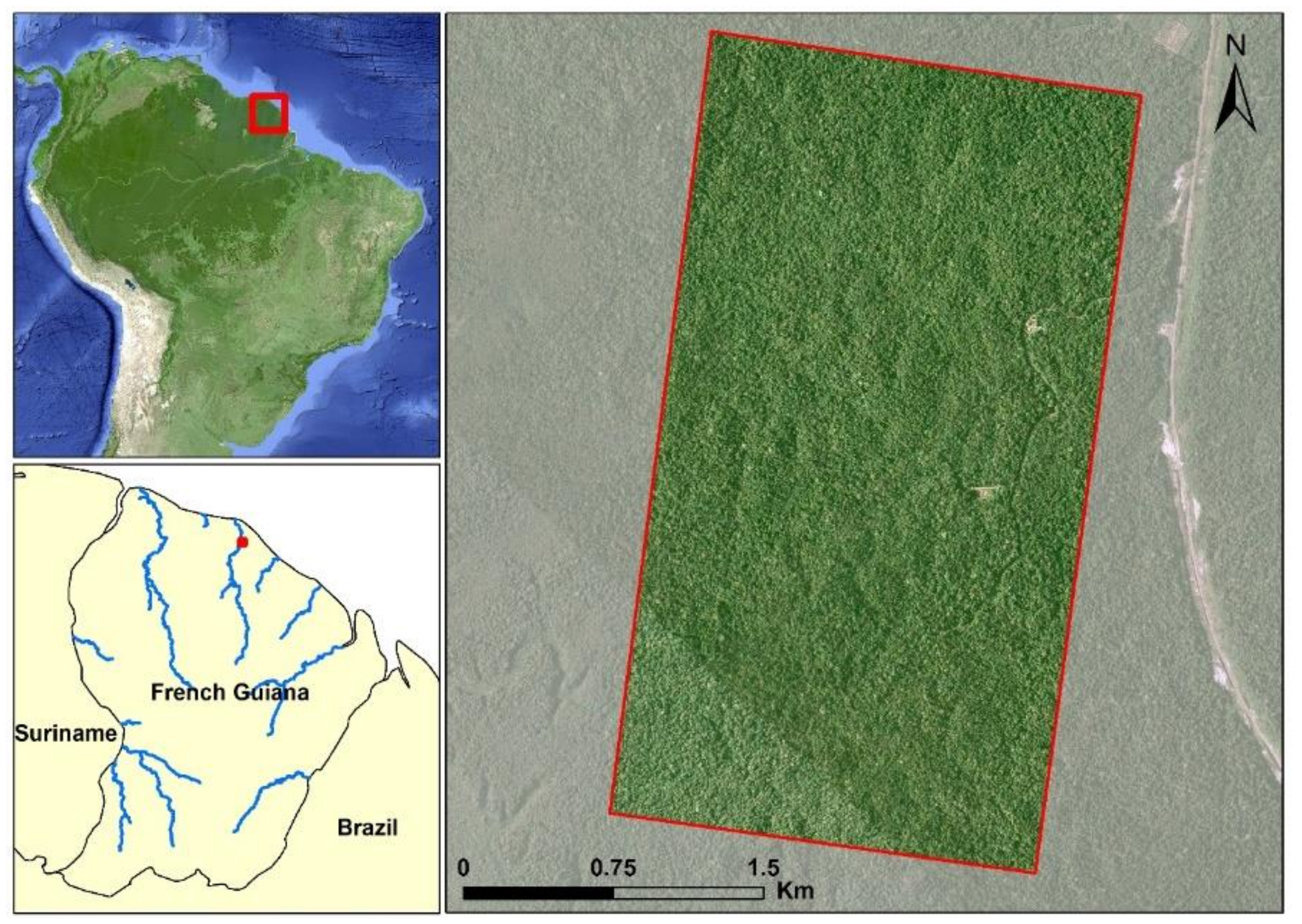
2.1.1. Study Area

The test site is located in French Guiana, near the town of Kourou, on the northern margin of the Guiana Shield, as shown in Figure 1. The surveyed site (52°55′55′′W and 5°16′9′′N) has an area of about 8 km² (2 km × 4 km). It is a typical Amazonian landscape with a hilly relief, a very dense hydrographic network and a dense rainforest. The area has practically no anthropic activities except the presence of a few small buildings. Over this site were acquired P-band airborne radar data in the framework of the ESA TropiSAR campaign [17] for the preparation of the BIOMASS space mission.

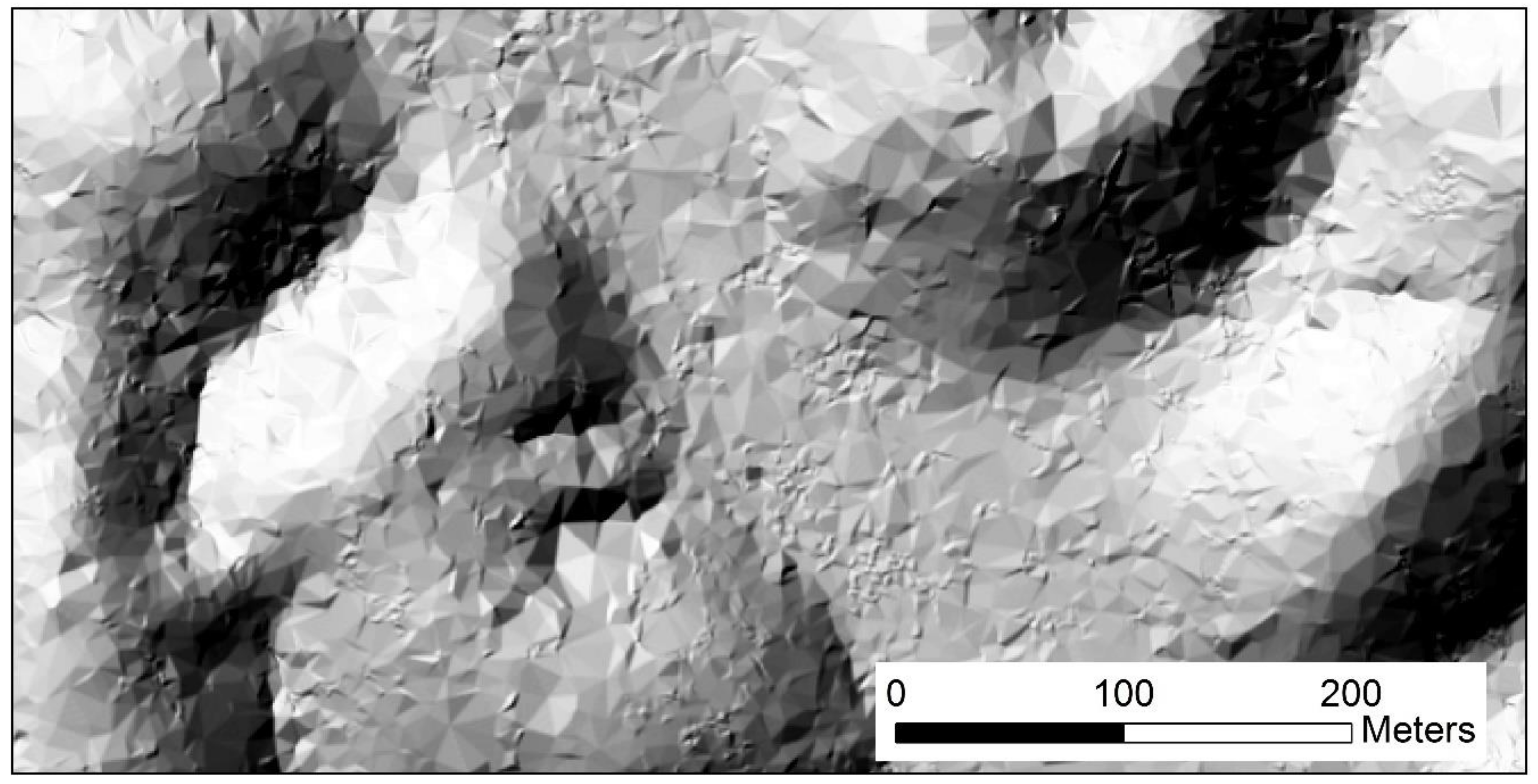
2.1.2. Lidar DTM

The lidar DTM, used as a reference, is produced using a small-footprint lidar system. The data was collected in 2009 by Altoa company (Cayenne, French Guiana) using a helicopter-mounted RIEGL LMS-280i (wavelength 0.9 μm) with a ground point density of about 0.1 point/m² [43]. The points representing the ground were interpolated into a triangulated irregular network (TIN), and the final DTM was resampled to a 1 m raster grid.

Airborne lidar is widely used for providing 3D surveys of the forest structure and the underlying topography in forested areas [44,45,46]. The altimetric accuracy is generally decimetric and depends on the morphology and the land cover. For example, in [44], the elevation accuracy of this technique ranges from 17 cm (open areas) to 26 cm (in forests). The lower density of ground points in the forest slightly increases the position error and creates shape errors due to the interpolation effect over longer distances (as shown in Figure 2 in the case of the TIN interpolation), which could bias the results of slope accuracy assessment. Furthermore, a considerable number of sinks exist along the watercourses, which can also alter the extracted stream network if not corrected. In spite of these artifacts, the overall high accuracy of the lidar DTM allows us to consider it as a reference to validate the P-band DTM. The radar and lidar campaigns both took place in 2009, so we consider that no change happened in the landscape.

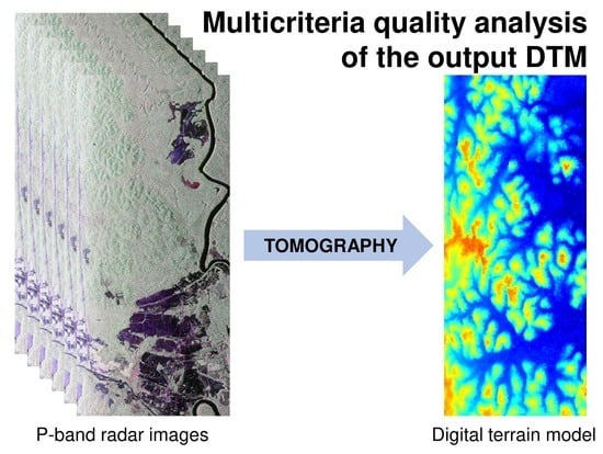
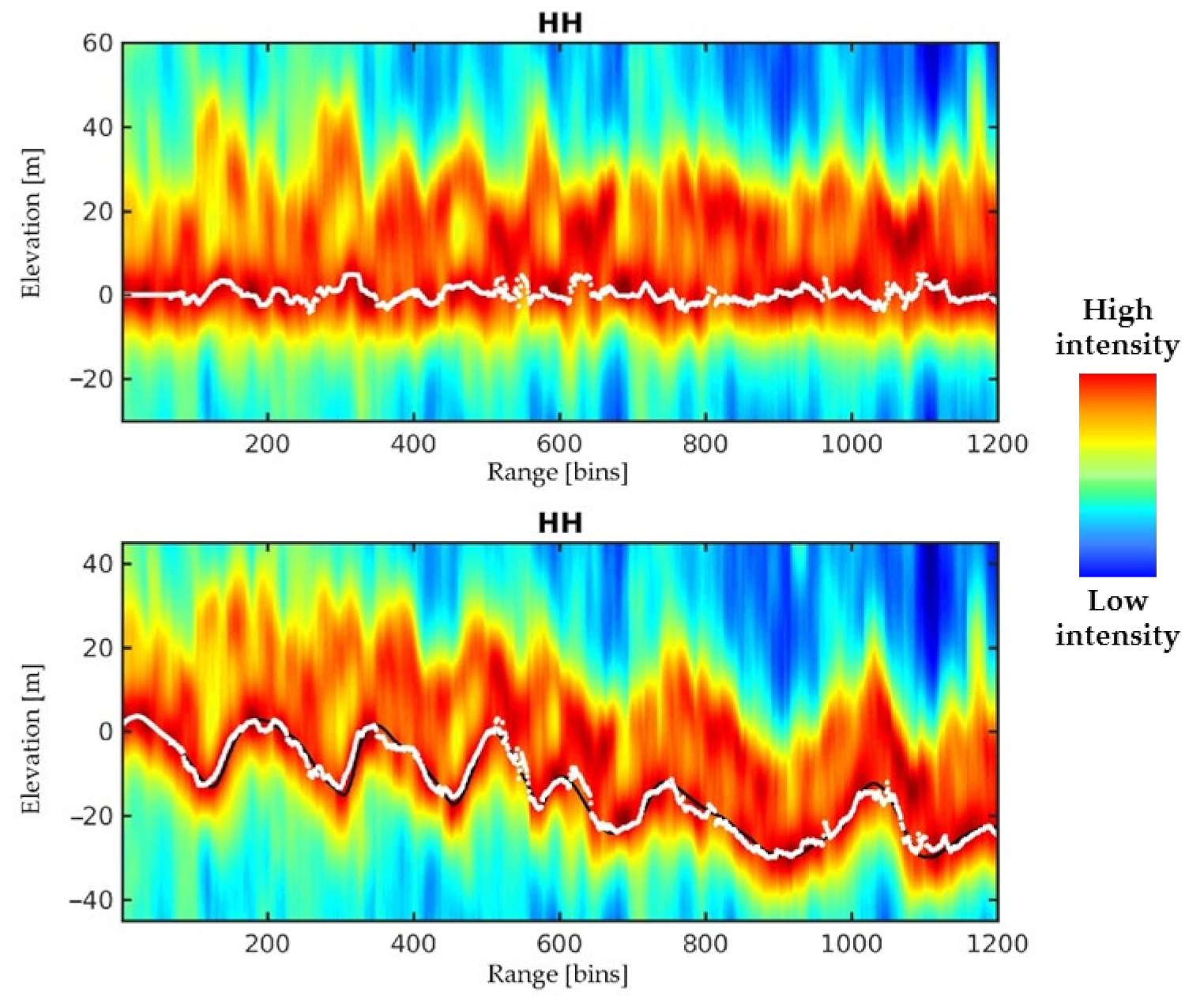
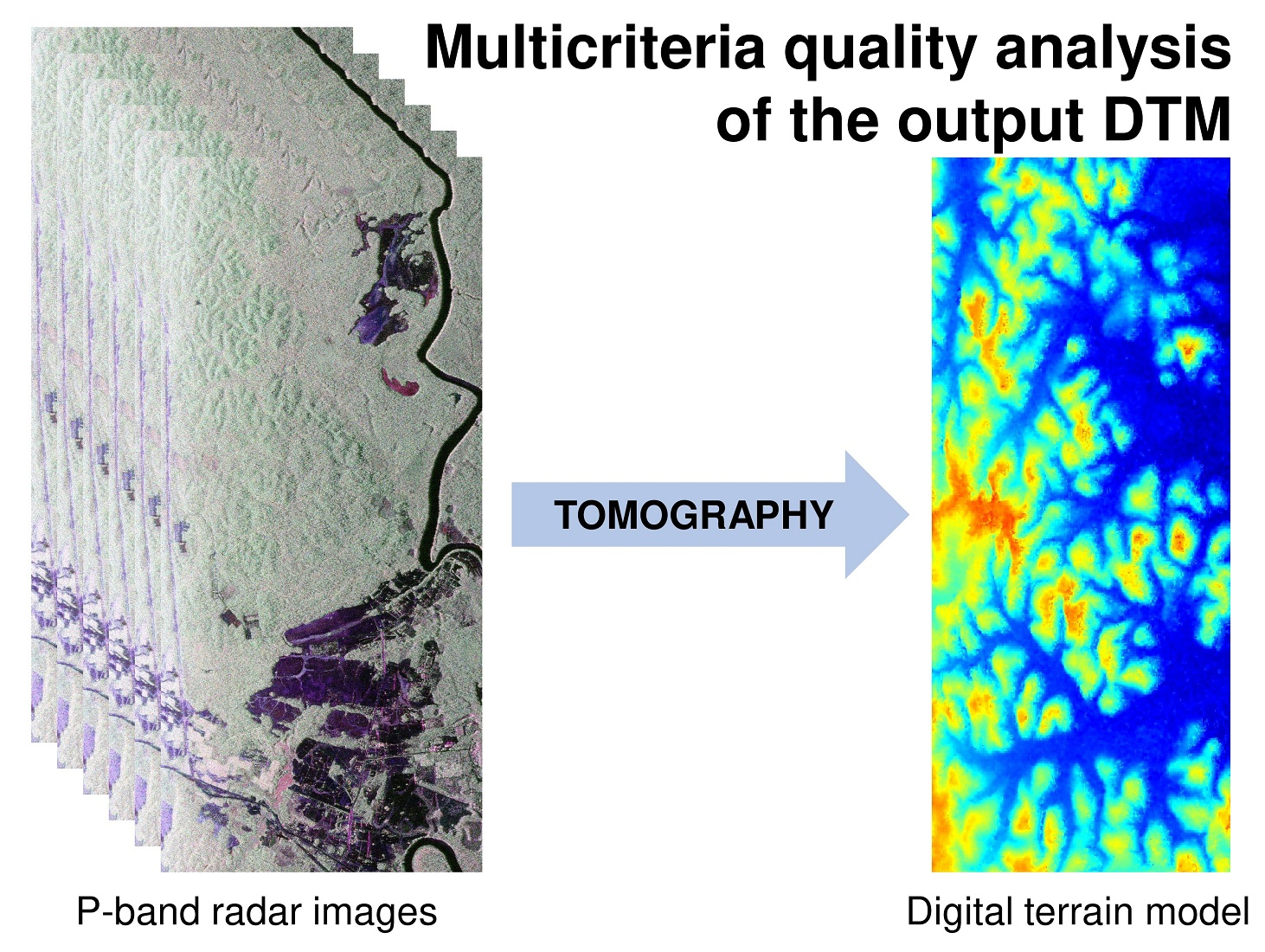
2.1.3. P-Band DTM

The SAR data processed in the frame of this study were measured in 2009 by the SETHI sensor by ONERA (Palaiseau, France) and consist of a set of 6 fully polarimetric images acquired in a repeat-pass multi-baseline InSAR mode at the P-band. The emitted radar signals occupy a spectral domain centered around ${\mathrm{f}}_{\mathrm{c}}=397.5 \mathrm{MHz}$, and the dimensions of the processed 2D spectrum led to spatial resolutions of 1.2 m and 1.5 m in the slant range and azimuth directions, respectively. A subset of the original stack, whose slant range and azimuth coordinates, delineated in Figure 3, coincide with those of the lidar DTM described below, has been selected. This sub-region, located in the near-to-medium range part of the original swath, is observed by the radar under an elevation angle, $\mathsf{\theta }$, ranging from 20 to 50 degrees, and is characterized by significant topographic features, with hills and valleys.

The principle of tomographic imaging, illustrated in Figure 4, is based on the use of coherent acquisitions performed from slightly shifted positions describing an additional aperture in the direction orthogonal to the radar line of sight. Classical 2D SAR imaging is known to be affected by a cylindrical ambiguity and merges responses originating from scatterers located at a similar distance from the radar, whatever their elevation. The coherent combination of several 2D SAR images acquired with spatial diversity allows the synthesis of 3D reflectivity maps using tomographic processing, which further refines original 2D resolution cells into 3D ones, whose extent in elevation, i.e., vertical resolution, depends on the length of the normalized multi-baseline aperture, the range distance and the carrier frequency [47]. Over the sub-region considered in this study, the vertical resolution ranges from approximately 16 m to 26 m, from near to far range. The polarization diversity may be used to further discriminate contributions having different polarimetric responses. In the case of 3D imaging, several studies showed that polarization could be efficiently used to separate the global response into two components, one of them being associated with the underlying ground response [30,48].

The processing chain set up in this study for estimating ground elevation using P-band tomographic SAR data may be described as follows. The first step consists of estimating residual interferometric phase terms, corresponding to equivalent antenna phase center position errors smaller than a signal’s wavelength, from the SAR images themselves using a phase error model, as proposed in [49]. The joint second-order statistics of the phase-corrected SAR images are then estimated using a sample multi-baseline PolInSAR, or simply PolTomoSAR, covariance matrix, given by:

$${\widehat{\mathit{R}}}_{PS}=\frac{1}{L}{\displaystyle \sum }_{l=1}^L{\mathit{k}}_{PS}\left(l\right){\mathit{k}}_{PS}^H\left(l\right)\in S{P}_{ℂ}^{M{N}_p\times M{N}_p}$$

(1)

where $S{P}_{ℂ}^{Q\times Q}$ is the set of complex-valued $\left(Q\times Q\right)$ positive semi-definite matrices, $M$ is the number of images, $N_p$ represents the number of polarimetric channels and $L$ is the number of realizations used to compute the covariance matrix estimate, which coincides with the maximum likelihood estimate in the case of normally distributed SLC echoes. For a given range-azimuth resolution cell, the acquired signals are gathered into a polarimetric and spatial vector, defined as:

$${\mathit{k}}_{PS}=\left[\begin{array}{c}{\mathit{k}}_1\\ ⋮\\ {\mathit{k}}_{N_p}\end{array}\right]\in {ℂ}^{M{N}_p\times 1}, \mathrm{with} {\mathit{k}}_i=\left[\begin{array}{c}{k}_{i_1}\\ ⋮\\ k_{i_M}\end{array}\right]\in {ℂ}^{M\times 1}$$

(2)

with $M=6$ images and $N_p=3$ polarization channels. The $L$ samples used to compute the covariance matrix are provided by a multi-dimensional $\left(N_{filt}\times N_{filt}\right)$ boxcar filter, with $N_{filt}=17$ pixels, empirically found as a good compromise preserving resolution and radiometric estimation accuracy, corresponding to $N_{eq}=200$ equivalent number of looks. The PolTomoSAR are then decomposed using algebraic approaches detailed in [48] and [50], and the component identified as representing the ground response is focused in the vertical direction using a non-parametric spectral analysis estimator [51]. The ground elevation is determined as the location in elevation corresponding to the maximum of the ground focused response. One may note that, in order to actually assess the intrinsic behavior of DTM estimated from SAR tomography at the P-band, no further processing step, such as smoothing filter regularization, is applied to the estimated elevation map. The final DEM was resampled at 1 m in both slant range and azimuth directions. The processing results are illustrated in Figure 5 with two tomographic profiles estimated in the range direction and displayed in absolute elevation coordinates and after compensation of the lidar DTM estimate.

2.2. Methods

2.2.1. DEM Quality Assessment Approaches

To assess the quality of a DEM, there are two major validation methods, called external and internal [52,53]. The external validation is based on the use of external reference data to assess positional and shape accuracies of the modeled terrain. The internal validation does not need any external data and aims to verify whether the modeled terrain is possible or at least realistic by checking if some physical and statistical rules are validated in the DEM [54,55].

In external validation, the accuracy of a DEM is generally assessed by characterizing the statistical distribution of the elevation difference between the DEM and a number of ground control points, using indicators such as mean, standard deviation, Root Mean Square (RMS), etc. [56]. However, these indicators do not guarantee the quality of terrain shapes, which depend on the accuracy of elevation derivatives such as slope, aspect or curvature to characterize landform elements [57]; most geoscientific applications of DEMs are based on these geomorphic parameters. As the shape descriptors are calculated using DEM values, elevation errors propagate through them and influence their accuracy. The influence of random elevation errors is greater on elevation derivatives as the derivation order increases, and an insignificant input error can, in some cases, give large errors in the derivatives [58,59]. Thus, it is possible to obtain high positional accuracy and a poor shape quality, and vice versa [53]. Indeed, the shape descriptor accuracy depends on both the elevation error and the spatial autocorrelation of this error [60]. Therefore, the overall DEM quality depends not only on the positional accuracy but also on shape accuracy [61].

The elevation error is a result of gross, systematic and random errors and is generally considered to be normally distributed [60,62]. To estimate this error, the elevation difference between the DEM and a sufficiently large sample of reference points is measured, and the RMS is calculated [63]. The value obtained characterizes the elevation quality but does not necessarily reveal the shape uncertainty [64]. Then, to assess the elevation error propagation through the shape descriptors, the spatial autocorrelation of the elevation error has to be evaluated [65]. Finally, an elevation error model for the DEM can be built using the elevation error and its spatial autocorrelation. The error propagation in the shape descriptors can then be assessed analytically when possible or numerically by using a Monte-Carlo simulation [58,66,67].

Different factors can affect the quality of a DEM, related to the production method and its production parameters but also to landscape characteristics [68]. For instance, the acquisition parameters and production parameters have a direct influence on the elevation and its derivatives [69,70,71]. Some production techniques produce errors that are more autocorrelated than others, which provide more accurate results for terrain shape modeling [56,66]. The error autocorrelation can be preserved by processing steps that reduce elevation noise, but this generally leads to degradation of the resolution so that the DTM can no longer depict the smallest terrain shapes. On the other hand, the terrain slope and aspect can also have an impact on the produced DEM [68,72].

Some shape descriptors are scale-free such as the closed depression volume and elevation [59,73], but most of them are scale-dependent [74,75], and their values and quality depend on the mesh size [67,76]. Thus, the choice of the mesh size must be defined according to the foreseen application to have the best results in terms of accuracy [77,78].

The external and internal validation methods used in this study are outlined in the following two sections.

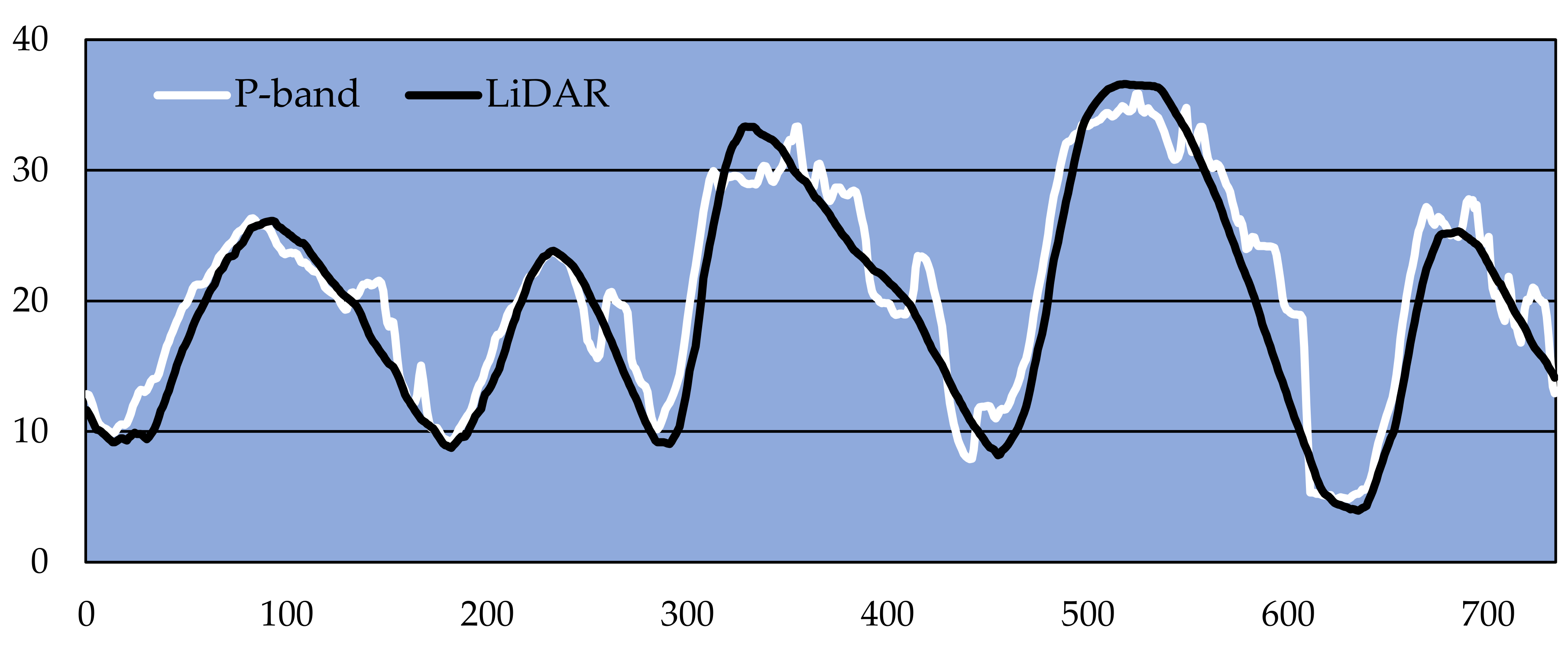
2.2.2. External Validation

External validation consists in comparing the DEM with higher quality external data, typically a set of ground control points or a higher accuracy DEM. The error analysis in this study is based on statistical indicators of the difference between the P-band and lidar DTMs. The overall error in a DEM is composed of different kinds of errors. As Equation (1) shows, the elevation modeled in a DEM (${\widehat{z}}_i$) is the sum of the true elevation on the terrain ($z_i$) with a systematic error or a bias (${\mu }_i$) and a random error [56,66,79]; this latter is composed of a spatially correlated term (${{\epsilon }^{\prime }}_i$) and a spatially white noise term (${{\epsilon }^{″}}_i$).

$${\widehat{z}}_i=z_i+{\mu }_i+{{\epsilon }^{\prime }}_i+{{\epsilon }^{″}}_i$$

(3)

In order to evaluate those errors, a list of quality criteria is used. The mean value of the difference between the P-band and lidar DTMs gives the bias between these two DTMs, whereas the standard deviation provides a relevant description of the random error.

$$\mu =\frac{1}{N}{{\displaystyle \sum }}_{i=1}^N({\widehat{z}}_i-z_i)$$

(4)

$$\sigma =\sqrt{\frac{1}{N}{\displaystyle \sum }_{i=1}^N{\left({\widehat{z}}_i-z_i\right)}^2-{\mu }^2}$$

(5)

The most used statistical indicator in DEM validation is the root mean square error (RMSE) of the elevation (Equation (4)), which includes both systematic and random errors, as shown in Equation (5).

$$\mathrm{RMSE}=\sqrt{\frac{1}{N}{\displaystyle \sum }_{i=1}^N{\left({\widehat{z}}_i-z_i\right)}^2}$$

(6)

$$\mathrm{RMSE}=\sqrt{{\mu }^2+{\sigma }^2}$$

(7)

The mean, standard deviation and RMSE are also calculated for the absolute slope to show the impact on the shape modeling, as it is the most used topographic index to quantify the terrain morphology. The slope is calculated using the third-order finite difference weighted by the reciprocal of squared distance [80] for all the DTMs with a 1 m mesh size. Since some parameters are scale-dependent, DEMs must have the same mesh size in order to be compared [74,75].

The autocorrelated part of the random error is evaluated at different lags, assuming stationary random error terms. It is calculated using the following formula.

$$r\left(h\right)=\frac{\frac{1}{n}{{\displaystyle \sum }}_{i=1}^n{d}_i\times d_{i+h}-\frac{1}{n}{{\displaystyle \sum }}_{i=1}^n{d}_i\times \frac{1}{n}{{\displaystyle \sum }}_{i=1}^n{d}_{i+h}}{\sqrt{\frac{1}{n}{{\displaystyle \sum }}_{i=1}^n{d}_i{}^2-{\left(\frac{1}{n}{{\displaystyle \sum }}_{i=1}^n{d}_i\right)}^2 }\times \sqrt{\frac{1}{n}{{\displaystyle \sum }}_{i=1}^n{d}_{i+h}{}^2-{\left(\frac{1}{n}{{\displaystyle \sum }}_{i=1}^n{d}_{i+h}\right)}^2}}$$

(8)

where n is the total number of point pairs, $d_i$ is the difference between the two DEMs at the position i, $d_{i+h}$ is the difference at the position i + h at a distance h (which is the lag) from the position i. In this study, the lag ranges from 1 to 20 pixels.

All the aforementioned indicators are calculated for the overall P-band DTM with regard to the lidar DTM. The influences of the landscape and the acquisition geometry on the quality of the DTM are analyzed, based on the slope, the effects of which have been widely studied for other techniques [68,72], as well as the aspect, the viewing angle and the local incidence angle.

2.2.3. Internal Validation

Internal validation consists of identifying the evidence of errors and artifacts in the DEM itself, revealed by the presence of unlikely or even impossible terrain shapes. This approach is based on the fact that topographic surfaces have universal properties, so that specific rules are fulfilled everywhere, and their non-satisfaction is considered a consequence of DEM errors. This rule-based approach can be applied without the need for external reference data and is based on both strong and weak requirements [41].

A strong requirement can be expressed by some physical rule, and a terrain that does not fulfill it is impossible. A well-known physical law is that water always goes down. Thus, the occurrence of sinks along the watercourses is a strong indicator of the presence of artifacts in the DEM [54]. The percentage of sinks and their mean depth, along with their spatial distribution, can therefore help provide the location and a quantitative indication of DEM errors.

A weak requirement can be expressed by a statistical rule, and a terrain that does not comply with this rule is improbable but not impossible. For example, terrains modeled by hydric erosion, which is the case of most continental surfaces, have a fractal behavior [81]. A consequence is that they respect Horton’s law, according to which the logarithm of the total number of streams of a given Strahler order decreases linearly as a function of the order [82]. A deviation from this law is also considered a consequence of DEM errors.

To apply this validation method, the percentage of sinks and the mean, standard deviation and RMS of their depth are first calculated. Then, the compliance of the rivers extracted from the DEM to Horton’s law is verified by the calculation of the R² coefficient of the cloud point fitting.

3. Results

3.1. External Validation

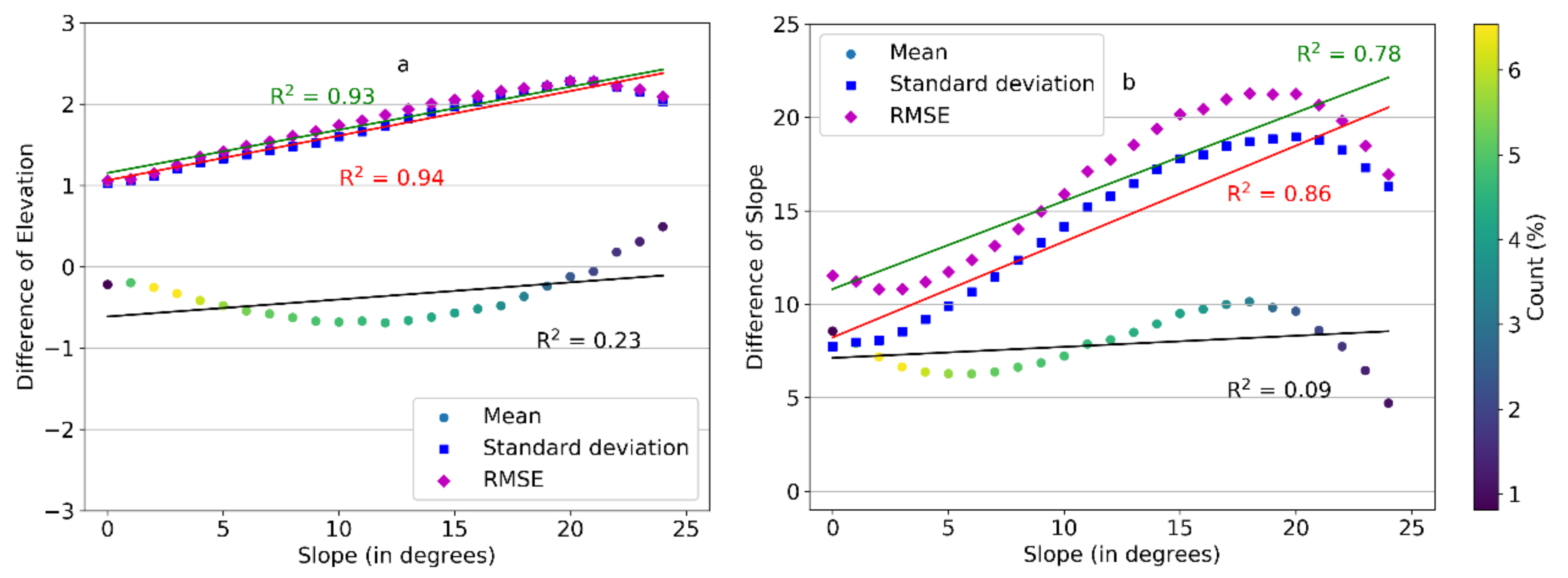
3.1.1. Elevation and Slope Errors

The comparison of the P-band radar DTM with the reference lidar DTM provides quality estimations in terms of elevation and slope accuracy.

In Figure 6, the mean value of the elevation error is negligible, whereas the standard deviation is less than 2 m, confirming the potential of P-band radar tomography in terms of absolute elevation accuracy. The slope is higher in the P-band DTM than in the lidar DTM of about 7° on average, and the slope error has a standard deviation and RMSE of about 14° and 16°, respectively. As shown in Section 3.2, these high values of slope error are due to artifacts produced by the application of a 17 × 17 boxcar filter during the tomographic covariance matrix estimation step. The use of smoother filters, with a Gaussian impulse response, for instance, would mitigate this effect [83]. A small region free from this artifact has a higher slope accuracy, i.e., an average slope and standard deviation of about 2°.

The autocorrelation (shown in Figure 7) is high over short distances due to the 17 × 17 boxcar estimation filter, with no significant difference between range and azimuth directions. It decreases as the distance increases, which is the usual behavior of DEM error autocorrelation as a consequence of Tobler’s first law of geography [84,85], and it remains higher in the azimuth direction. This suggests that the shapes are noisier in the range direction, as will be confirmed below.

To better understand the source of the elevation and slope errors, these were extracted according to the morphology of the terrain (slope and aspect), radar acquisition parameters (off-nadir angle and local incidence angle) and a combination of these.

Figure 8 shows the effects of terrain slope on the DTM quality in terms of elevation and slope errors, the reference slope being calculated using the lidar DTM. This figure shows that the mean elevation error is negligible whatever the slope and that the standard deviation increases linearly ($R^2>0.9$) with a difference of around 1 m between elevation errors obtained for the smallest and the steepest slope, which confirms the results obtained with other DTM production techniques [72,86,87]. The slope error also increases according to terrain slope to reach a maximum at around 20°, then it decreases. The standard deviation exhibits a slight increase, almost linear, for slopes less than 20°, which is not consistent with other theoretical studies that suggest a decreasing standard deviation of the slope with an increasing slope [67]. However, the influence of the slope has to be interpreted with care since it is likely to be combined with the influence of the radar viewing angle, as suggested by the following results.

The impact of the off-nadir angle is shown in Figure 9. According to this figure, the following can be observed:

-

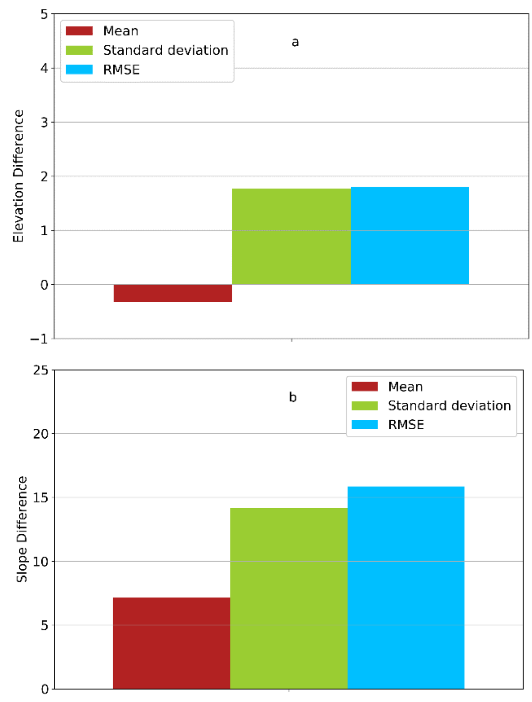
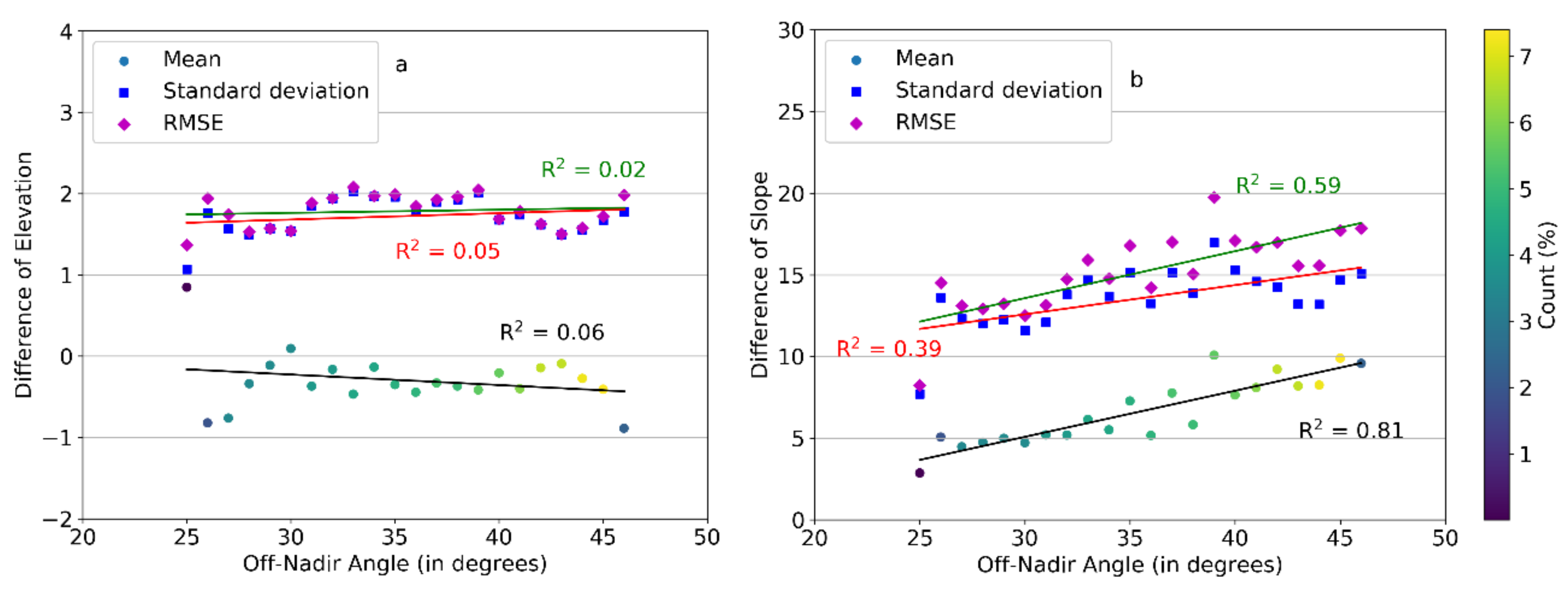
The mean value of elevation error is negligible, whatever the off-nadir angle. Similarly, the standard deviation is little influenced by this angle and fluctuates around 2 m.

-

The slope error (mean and standard deviation) is an increasing function of the off-nadir angle, and it reaches large values. This relationship is certainly related to the decrease of vertical resolution as the off-nadir angle rises.

Figure 10 shows the impact of the local incidence angle on elevation and slope errors. This figure shows the following:

-

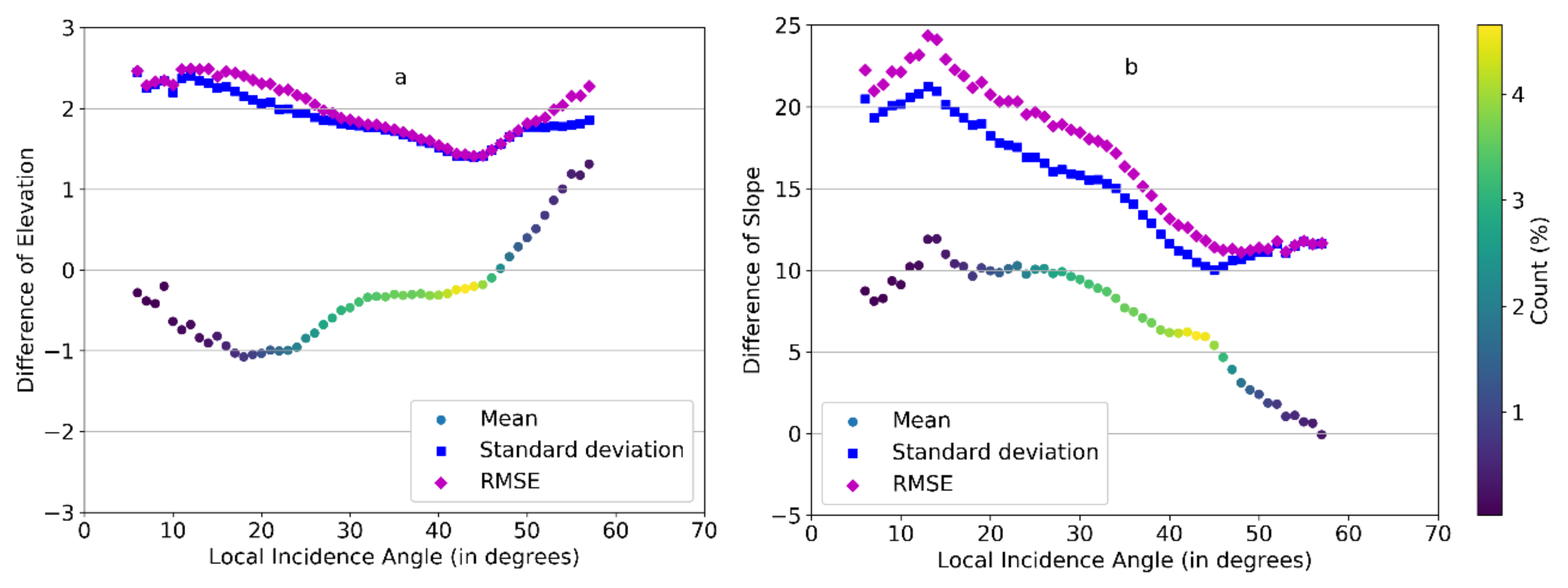
The mean elevation error is negligible for angles ranging between 30° and 45°, whereas the standard deviation decreases to reach a minimum for a 45° angle. As explained in [88,89,90], the double bounce reflection occurring between the ground and tree trunks is a very energetic and directional scattering mechanism, having a narrow scattering diagram centered around 45°. When the incidence angle reaches this range of values, the dominant double-bounce responses, whose phase center is exactly located at the ground level, can easily be perceived in tomograms and localized in elevation.

-

The mean and standard deviation of the slope error are maximum for small local incidence angles (10–20°), which may be explained both by the weaker contribution of double-bounce scattering and by loss of resolution in areas facing the radar, and they decrease as the local incidence angle increases.

Figure 11 describes the influence of the terrain aspect, i.e., the azimuth direction of the maximum slope, on the elevation and slope errors, considering the flight direction (bottom to top). According to this figure:

-

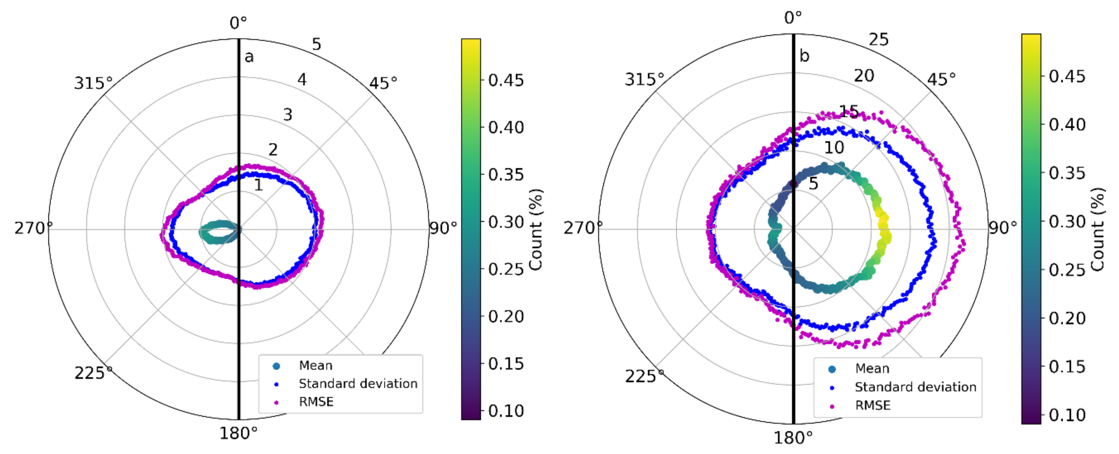
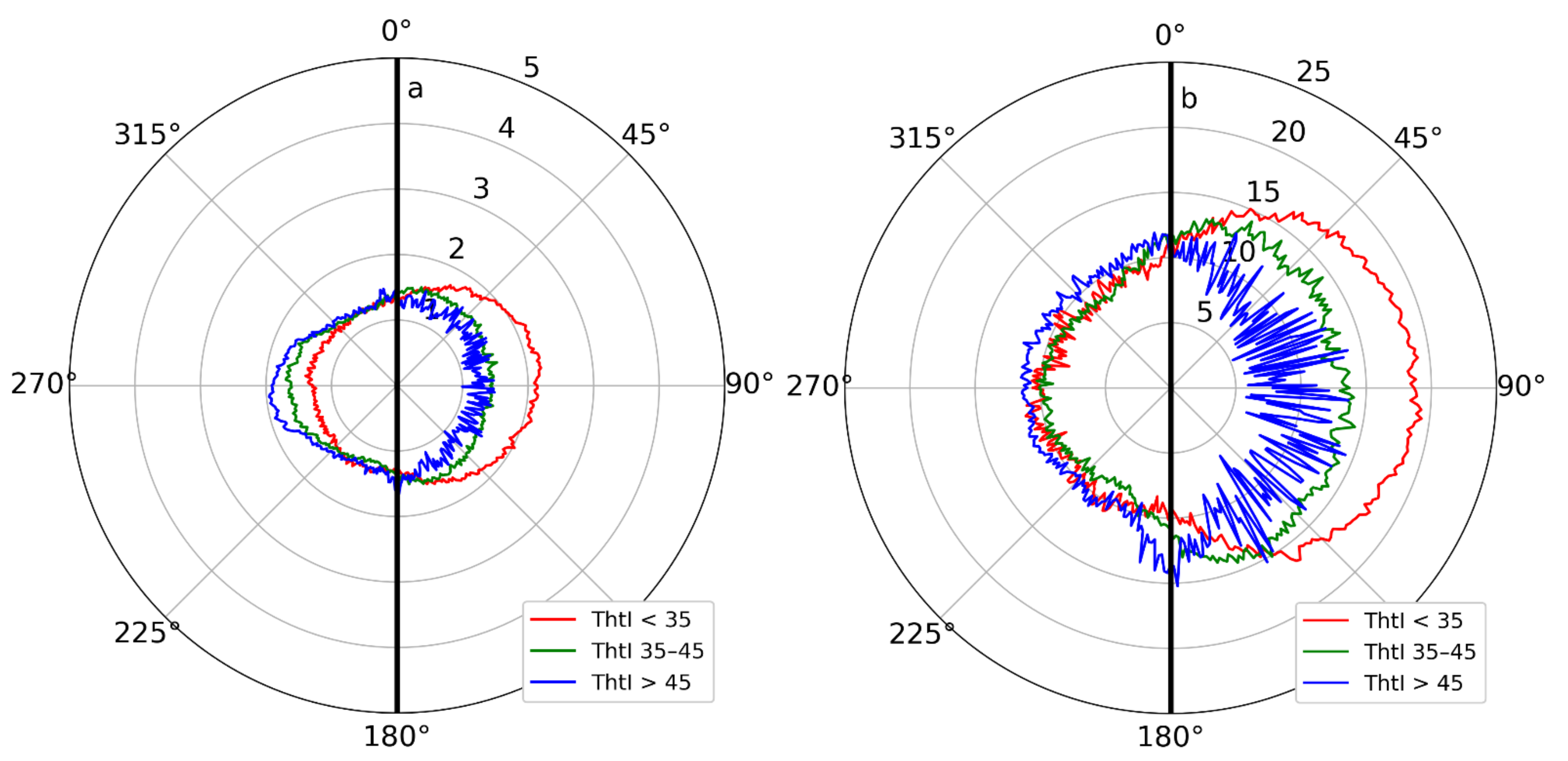
The mean error in elevation is maximum for slopes facing the radar antenna, probably related to a loss of vertical resolution, while it is almost zero for slopes in the other direction. The standard deviation is higher in the range direction than in the azimuth direction.

-

The slope mean error has the opposite behavior, with a maximum in the areas oriented away from the radar. The standard deviation has the same behavior.

To assess the impact of slopes and local incidence angles, the standard deviation of both elevation and slope are plotted against those parameters, and the results are shown in Figure 12 and Figure 13. According to these figures, the following can be observed:

-

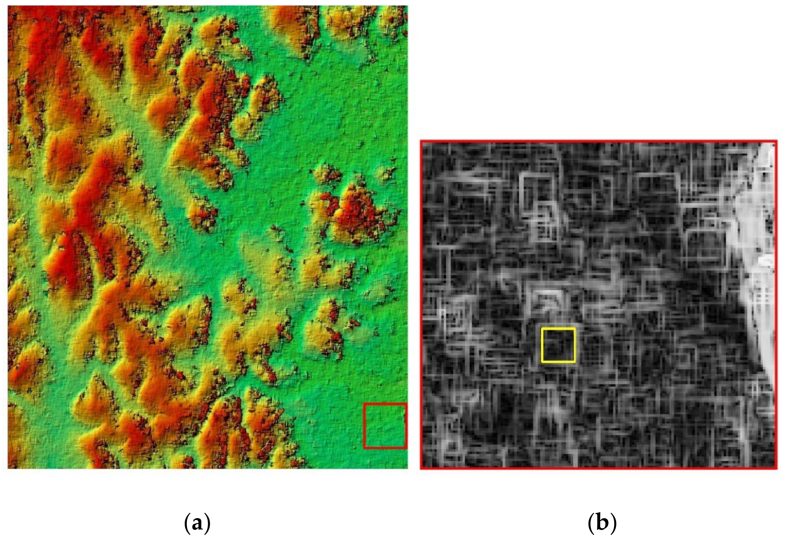
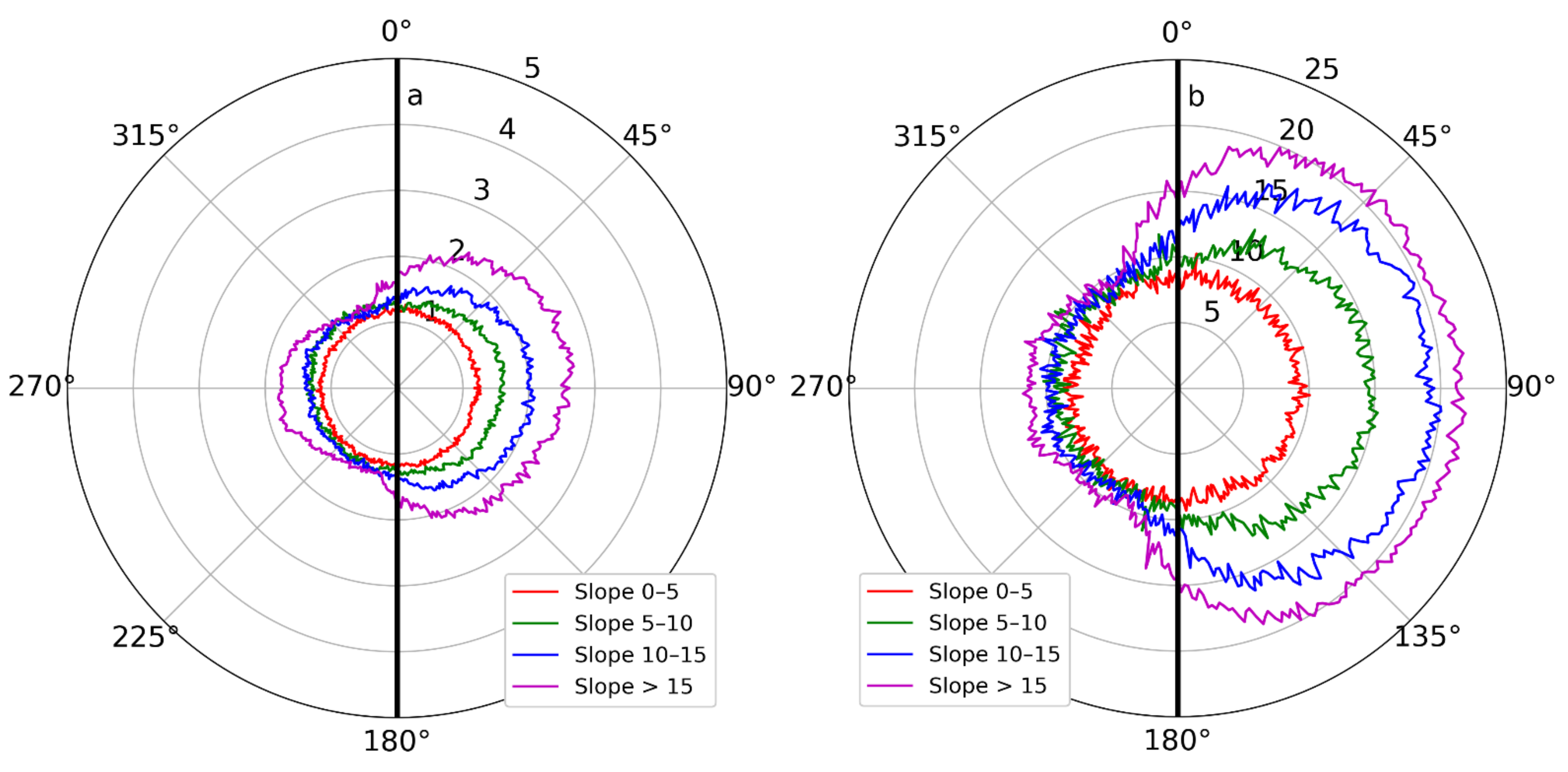
The standard deviation of the elevation error is negligible and isotropic in flat areas, and it gets higher for larger slope values, mainly for slopes facing away from the radar, which is due to a lack of ground response, with either single- or double-bounce contributions, while it preserves an almost constant value for slopes facing the radar, as confirmed by the profile shown in Figure 14.

-

For the largest slope values, the standard deviation is high. The largest local incidence angles produce the maximum error in areas facing the radar, characterized by a lower vertical resolution and by double-bounce scattering contributions with low intensity. The smallest angles produce the highest error in areas facing away from the radar. The intermediate angles (35–45°) lead to the best trade-off, as already shown in Figure 10.

-

The standard deviation of the slope error shows a similar tendency as the elevation error with respect to the slope and aspect. For the same reasons, the results are less reliable for steep slopes facing away from the radar.

All of those results suggest the importance of the radar acquisition parameters and their interaction with the terrain morphology as well as the flight direction in the quality of the produced DEM, specifically in forested areas.

3.2. Internal Validation

The first stage of internal validation is a visual control of the data. Figure 15 shows a combined hypsometry-hillshade representation of the P-band DTM, revealing the presence of random errors in the DTM, as well as systematic artifacts in its slope, due to the use of a raw boxcar filter for estimating the TomoSAR covariance matrix. Using a smoother filtering pattern should reduce this undesirable effect.

Figure 16 shows the variation of the number of streams (in logarithmic scale) as a function of the Strahler order for the streams extracted from the P-band DTM. This graph allows us to verify that the DTM respects Horton’s law, according to which the logarithm of the number of streams decreases linearly as a function of the Strahler order. Thus, a deviation from this law may be interpreted as due to the presence of an error and, therefore, the R² can be used as a quality criterion for the DEM [41]. As expected, the extracted streams show a linear decrease even for the smallest Strahler orders, which are generally more likely to be affected by noise, and the R², suggesting a higher quality of DTM shapes.

Sinks are obstacles in a DTM that prevent the extraction of a reliable and continuous stream network. They are a consequence of the presence of elevation errors in a DTM, and most DTMs include some.

Table 1. Percentage and depth of sinks in P-band DTMs.

Percentage of Sinks (%)		2.02%
Depth of sinks	Mean (m)	0.38
	Standard deviation (m)	0.60
	RMS (m)	0.71

shows the percentage and depth of those sinks in the P-band DTM. The percentage of the sinks is small (~2%), and the depth of those sinks is less than the elevation RMSE. This implies that the P-band DTM has a good agreement with the physical rule that the water always flows downward.

The results show that the shapes of the DTM are in agreement with the expected behavior of most continental surfaces.

4. Discussion

The results of the previous section have shown the potential of a DTM obtained by tomographic processing of P-band airborne radar data while revealing and explaining its limitations.

Our conclusions are based on the study of a particular case and can only be generalized with caution. For example, the study area has a moderate relief which does not allow predicting the performance to be expected from similar data on a mountainous landscape. In addition, we considered the case of a homogeneous forest, different from many terrestrial landscapes where the diversity of vegetation cover would have made the analysis more complex.

Our study is limited, in particular, by the small size of the study area, although the number of points is statistically very significant, and by the fact that we use lidar data as a reference, which has its own error. Indeed, the lidar DTM is highly smoothed due to the interpolation of ground points (which are less dense under forests), so that the slopes are underestimated, while the radar DTM has artifacts and noise that overestimate the slopes; the slope errors that we have calculated are therefore partly attributable to the lidar data. This is what makes the internal validation so interesting, as it allows us to detect DTM errors without the need for reference data. By proposing a multicriteria analysis, which combines requirements on the accuracy of heights and slopes and with respect to shapes, we thus obtain very complete results on the quality of a DTM, which is the original part of our contribution.

It should be noted that this study was based on radar data in slant range geometry, which is not the common geometry of classical DEM products. Although it leads to local variations in range resolution, this choice allows a more intrinsic evaluation of the performance of P-band tomography since it excludes the influence of the projection from slant to ground range or any other resampling step. In other words, the evaluation is based on a raw DTM, resulting from the two basic steps of DTM production, namely, the P-band radar data acquisition and the tomographic processing, without any subsequent post-processing.

Despite these limitations, this study is a basis for further work over larger areas and focuses on more diverse configurations, especially in terms of terrain topography, vegetation cover or acquisition parameters. In the case of the BIOMASS mission, those parameters are different and should give different results. Indeed, the radar bandwidth (6 MHz giving a 25 m range resolution) will not give access to the same topographic features, although the computational algorithm or the overall trends related to physical interactions at P-band (central frequency close to 400 MHz) remain very similar. Specific tomographic techniques will probably have to be implemented in order to cope with the low resolution and low dimensionality of the data [91]. In addition, it is also worth reminding that the exploitation of BIOMASS data will enable the combination of ascending and descending passes, which would significantly improve the mitigation of slant range geometrical effects and motivate further studies based on such configurations. The multicriteria analysis proposed in our study will then have to be conducted with a different interpretation.

5. Conclusions

The study presented in this paper provides an overall quality assessment of a digital elevation model produced by airborne P-band polarimetric SAR tomography in tropical rainforests, based on two validation approaches, namely, an external validation based on the comparison with a lidar DTM considered as a reference, and an internal validation based on the assessment of shape realism. The main conclusions of this multicriteria quality assessment are as follows:

• The P-band radar DTM has a negligible bias, and the elevation RMSE is around 2 m.
• The slope is overestimated with an average error of 7° and a standard deviation of 14°, mainly due to a processing artifact for which easy and direct solutions exist (2° and 2°, respectively, in flat artifact-free areas).
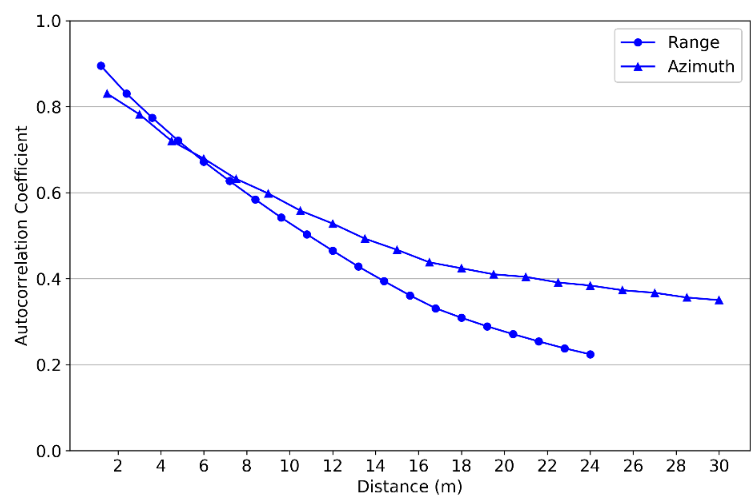
• The elevation and slope errors are more important in the range direction than in the azimuth direction, given the intrinsic effects of the radar slant range geometry.
• The difference between the P-band DTM and the lidar DTM is more important on steep slopes (maximum error around 18–20°); on slopes facing the sensor, the P-band is above the lidar (positive difference), while on slopes looking away from the sensor, the P-band is most often below the lidar (negative difference). In areas with small slopes, the difference is negligible (for both the mean and standard deviation). This is due to the double bounce effect, whose amplitude is maximal for an incidence angle lying close to 45° and over flat areas, over which the tree trunks and the ground are orthogonal. As the terrain slope increases, the error increases due to three effects:

  -

  The loss of resolution for slopes facing the radar, which produces an almost constant error;

  -

  A significant reduction of the amplitude of double-bounce scattering;

  -

  A lack of ground response, with either single- or double-bounce contributions, over slopes facing away from the radar.

• The off-nadir angle has little effect on the elevation error, while the mean and standard deviation of the slope error increase as a function of the off-nadir angle.
• The local incidence angle has little effect on the elevation error, while the mean and standard deviation of the slope error decrease as a function of the local incidence angle.
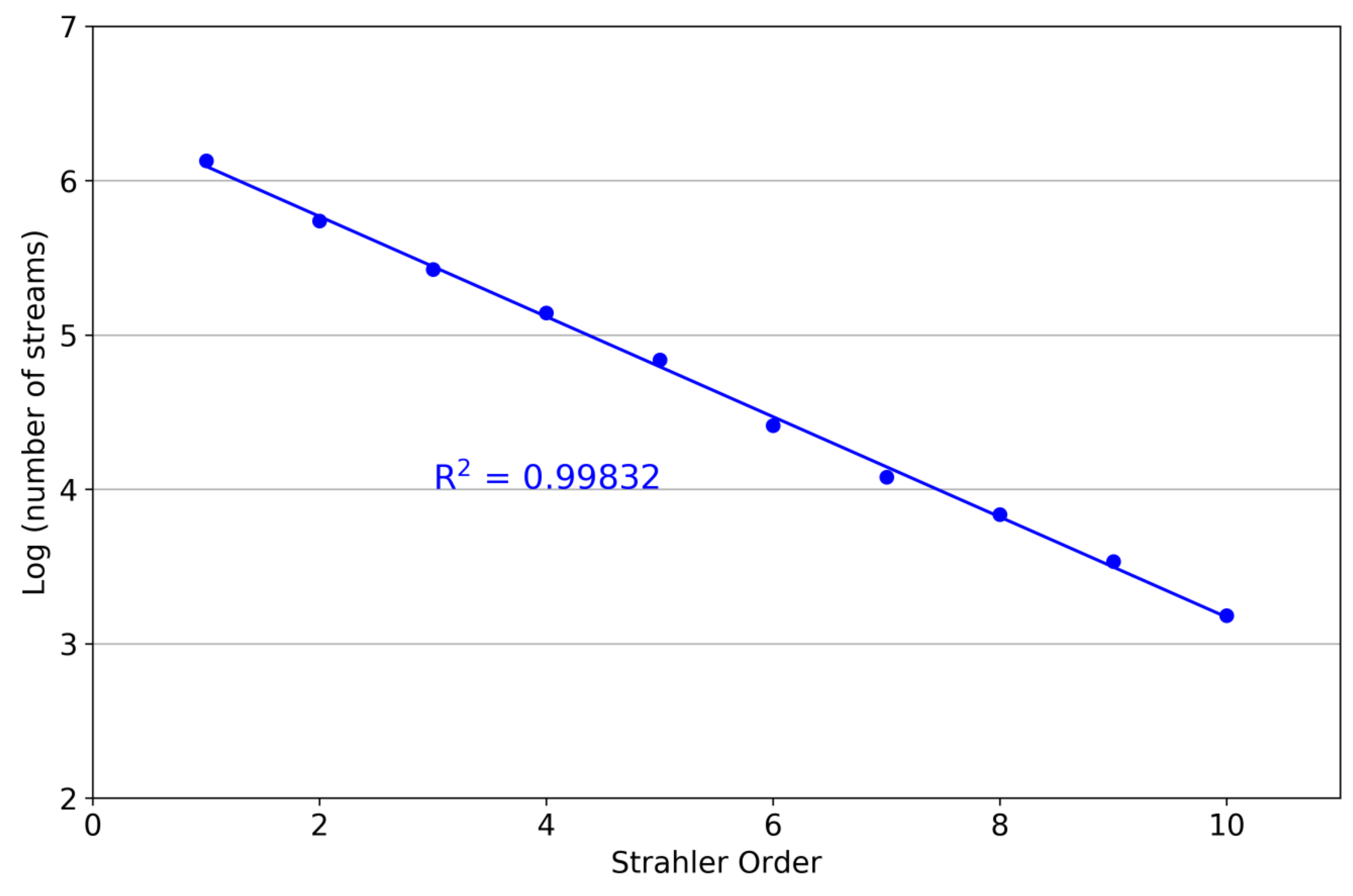
• Internal validation shows that the hydrography is well preserved, with few (2%) and shallow sinks (0.7 m RMS) and good compliance with Horton’s law.

These results are based on the analysis of a particular dataset over a small area with a specific landscape. They will be consolidated by further studies over larger areas with variable morphologies. This multicriteria accuracy assessment shows the importance of using ad hoc quality criteria, as proposed in this study, and the high potential of the P-Band SAR data in depicting the topography under forests in comparison to state-of-the-art lidar reference, although limited by the slant range geometry for which the combination of ascending/descending passes could solve the problem, and this could be very meaningful in spaceborne acquisitions such as in BIOMASS mission.

References

- Hengl, T.; Reuter, H.I. Geomorphometry: Concepts, Software, Applications; Elsevier: Amsterdam, The Netherlands, 2009; ISBN 978-0-12-374345-9. [Google Scholar]
- Polidori, L.; Caldeira, C.R.T.; Smessaert, M.; Hage, M.E. Digital Elevation Modeling through Forests: The Challenge of the Amazon. Acta Amaz. 2022, 52, 69–80. [Google Scholar] [CrossRef]
- Liu, X. Airborne LiDAR for DEM Generation: Some Critical Issues. Prog. Phys. Geogr. Earth Environ. 2008, 32, 31–49. [Google Scholar] [CrossRef]
- Maguya, A.S.; Junttila, V.; Kauranne, T. Algorithm for Extracting Digital Terrain Models under Forest Canopy from Airborne LiDAR Data. Remote Sens. 2014, 6, 6524–6548. [Google Scholar] [CrossRef]
- Štular, B.; Lozić, E.; Eichert, S. Airborne LiDAR-Derived Digital Elevation Model for Archaeology. Remote Sens. 2021, 13, 1855. [Google Scholar] [CrossRef]
- Baltsavias, E.P. A Comparison between Photogrammetry and Laser Scanning. ISPRS J. Photogramm. Remote Sens. 1999, 54, 83–94. [Google Scholar] [CrossRef]
- Leberl, F. Radargrammetric Image Processing; Artech House: Norwood, MA, USA, 1989; ISBN 978-0-89006-273-9. [Google Scholar]
- Capaldo, P.; Crespi, M.; Fratarcangeli, F.; Nascetti, A.; Pieralice, F. High-Resolution SAR Radargrammetry: A First Application With COSMO-SkyMed SpotLight Imagery. IEEE Geosci. Remote Sens. Lett. 2011, 8, 1100–1104. [Google Scholar] [CrossRef]
- Toutin, T.; Blondel, E.; Clavet, D.; Schmitt, C. Stereo Radargrammetry With Radarsat-2 in the Canadian Arctic. IEEE Trans. Geosci. Remote Sens. 2013, 51, 2601–2609. [Google Scholar] [CrossRef]
- Paquerault, S.; Maitre, H.; Nicolas, J. Radarclinometry for ERS-1 Data Mapping. In Proceedings of the IGARSS ’96. 1996 International Geoscience and Remote Sensing Symposium, Lincoln, NE, USA, 31 May 1996; Volume 1, pp. 503–505. [Google Scholar]
- Le Hégarat-Mascle, S.; Zribi, M.; Ribous, L. Retrieval of Elevation by Radarclinometry in Arid or Semi-arid Regions. Int. J. Remote Sens. 2005, 26, 2877–2899. [Google Scholar] [CrossRef]
- Zebker, H.A.; Goldstein, R.M. Topographic Mapping from Interferometric Synthetic Aperture Radar Observations. J. Geophys. Res. Solid Earth 1986, 91, 4993–4999. [Google Scholar] [CrossRef]
- Farr, T.G.; Rosen, P.A.; Caro, E.; Crippen, R.; Duren, R.; Hensley, S.; Kobrick, M.; Paller, M.; Rodriguez, E.; Roth, L.; et al. The Shuttle Radar Topography Mission. Rev. Geophys. 2007, 45, 1–33. [Google Scholar] [CrossRef] [Green Version]
- Fu, H.; Wang, C.; Zhu, J.; Xie, Q.; Zhang, B. Estimation of Pine Forest Height and Underlying DEM Using Multi-Baseline P-Band PolInSAR Data. Remote Sens. 2016, 8, 820. [Google Scholar] [CrossRef]
- Fu, H.; Zhu, J.; Wang, C.; Wang, H.; Zhao, R. Underlying Topography Estimation over Forest Areas Using High-Resolution P-Band Single-Baseline PolInSAR Data. Remote Sens. 2017, 9, 363. [Google Scholar] [CrossRef]
- D’Alessandro, M.M.; Tebaldini, S. Digital Terrain Model Retrieval in Tropical Forests Through P-Band SAR Tomography. IEEE Trans. Geosci. Remote Sens. 2019, 57, 6774–6781. [Google Scholar] [CrossRef]
- Dubois-Fernandez, P.; Oriot, H.; Coulombeix, C.; Cantalloube, H.; Plessis, O.R.D.; Toan, T.L.; Daniel, S.; Chave, J.; Blanc, L.; Davidson, M. TropiSAR, a SAR Data Acquisition Campaign in French Guiana. In Proceedings of the 8th European Conference on Synthetic Aperture Radar, Aachen, Germany, 7–10 June 2010; pp. 1–4. [Google Scholar]
- Huang, Y.; Ferro-Famil, L.; Lardeux, C. Polarimetric SAR Tomography of Tropical Forests at P-Band. In Proceedings of the 2011 IEEE International Geoscience and Remote Sensing Symposium, Vancouver, BC, Canada, 24–29 July 2011; pp. 1373–1376. [Google Scholar]
- El Idrissi Essebtey, S.; Villard, L.; Borderies, P.; Koleck, T.; Monvoisin, J.P.; Burban, B.; Le Toan, T. Temporal Decorrelation of Tropical Dense Forest at C-Band: First Insights From the TropiScat-2 Experiment. IEEE Geosci. Remote Sens. Lett. 2020, 17, 928–932. [Google Scholar] [CrossRef]
- Zink, M.; Fiedler, H.; Hajnsek, I.; Krieger, G.; Moreira, A.; Werner, M. The TanDEM-X Mission Concept. In Proceedings of the 2006 IEEE International Symposium on Geoscience and Remote Sensing, Denver, CO, USA, 31 July–4 August 2006; pp. 1938–1941. [Google Scholar]
- Tebaldini, S.; Ferro-Famil, L. SAR Tomography from Bistatic Single-Pass Interferometers. In Proceedings of the 2017 IEEE International Geoscience and Remote Sensing Symposium (IGARSS), Worth, TX, USA, 23 July 2017; pp. 133–136. [Google Scholar]
- Hensley, S.; Van Zyl, J.; Lavalle, M.; Neumann, M.; Michel, T.; Muellerschoen, R.; Pinto, N.; Simard, M.; Moghaddam, M. L-Band and P-Band Studies of Vegetation at JPL. In Proceedings of the 2015 IEEE Radar Conference, Marriott Crystal Gateway, Arlington, VA, USA, 27 October 2015; pp. 516–520. [Google Scholar]
- Le Toan, T.; Quegan, S.; Davidson, M.W.J.; Balzter, H.; Paillou, P.; Papathanassiou, K.; Plummer, S.; Rocca, F.; Saatchi, S.; Shugart, H.; et al. The BIOMASS Mission: Mapping Global Forest Biomass to Better Understand the Terrestrial Carbon Cycle. Remote Sens. Environ. 2011, 115, 2850–2860. [Google Scholar] [CrossRef]
- Quegan, S.; Le Toan, T.; Chave, J.; Dall, J.; Exbrayat, J.-F.; Minh, D.H.T.; Lomas, M.; D’Alessandro, M.M.; Paillou, P.; Papathanassiou, K.; et al. The European Space Agency BIOMASS Mission: Measuring Forest above-Ground Biomass from Space. Remote Sens. Environ. 2019, 227, 44–60. [Google Scholar] [CrossRef]
- Tebaldini, S.; Mariotti D’Alessandro, M.; Dinh, H.T.M.; Rocca, F. P Band Penetration in Tropical and Boreal Forests: Tomographical Results. In Proceedings of the 2011 IEEE International Geoscience and Remote Sensing Symposium, Vancouver, BC, Canada, 24–29 July 2011; pp. 4241–4244. [Google Scholar]
- El Idrissi Essebtey, S.; Villard, L.; Borderies, P.; Koleck, T.; Burban, B.; Le Toan, T. Long-Term Trends of P-Band Temporal Decorrelation Over a Tropical Dense Forest-Experimental Results for the BIOMASS Mission. IEEE Trans. Geosci. Remote Sens. 2022, 60, 1–15. [Google Scholar] [CrossRef]
- Shiroma, G.H.X.; de Macedo, K.A.C.; Wimmer, C.; Moreira, J.R.; Fernandes, D. The Dual-Band PolInSAR Method for Forest Parametrization. IEEE J. Sel. Top. Appl. Earth Obs. Remote Sens. 2016, 9, 3189–3201. [Google Scholar] [CrossRef]
- Fu, H.Q.; Zhu, J.J.; Wang, C.C.; Zhao, R.; Xie, Q.H. Underlying Topography Estimation Over Forest Areas Using Single-Baseline InSAR Data. IEEE Trans. Geosci. Remote Sens. 2019, 57, 2876–2888. [Google Scholar] [CrossRef]
- Ferro-Famil, L.; Huang, Y.; Pottier, E. Principles and Applications of Polarimetric SAR Tomography for the Characterization of Complex Environments. In VIII Hotine-Marussi Symposium on Mathematical Geodesy; Sneeuw, N., Novák, P., Crespi, M., Sansò, F., Eds.; Springer International Publishing: Cham, Germany, 2016; pp. 243–255. [Google Scholar]
- Aghababaei, H.; Ferraioli, G.; Ferro-Famil, L.; Huang, Y.; Mariotti D’Alessandro, M.; Pascazio, V.; Schirinzi, G.; Tebaldini, S. Forest SAR Tomography: Principles and Applications. IEEE Geosci. Remote Sens. Mag. 2020, 8, 30–45. [Google Scholar] [CrossRef]
- Chandra, M.; Hounam, D. Feasibility of a Spaceborne P-Band SAR for Land Surface Imaging; VED: Friedrichshafen, Germany, 1998. [Google Scholar]
- Villard, L.; Le Toan, T.; Ho Tong Minh, D.; Mermoz, S.; Bouvet, A. 9—Forest Biomass from Radar Remote Sensing. In Land Surface Remote Sensing in Agriculture and Forest; Baghdadi, N., Zribi, M., Eds.; Elsevier: Amsterdam, The Netherlands, 2016; pp. 363–425. ISBN 978-1-78548-103-1. [Google Scholar]
- Polidori, L.; Koleck, T.; Villard, L.; El Hage, M.; Paillou, P.; Le Toan, T. Cartographier Le Relief Sous Les Forêts et Le Substrat Sous Les Déserts de Sable: Les Attentes de La Mission Radar Biomass. Rev. XYZ 2018, 154, 56–61. [Google Scholar]
- Papathanassiou, K.P.; Cloude, S.R.; Pardini, M.; Quiñones, M.J.; Hoekman, D.; Ferro-Famil, L.; Goodenough, D.; Chen, H.; Tebaldini, S.; Neumann, M.; et al. Forest Applications. In Polarimetric Synthetic Aperture Radar: Principles and Application; Hajnsek, I., Desnos, Y.-L., Eds.; Remote Sensing and Digital Image Processing; Springer International Publishing: Cham, Germany, 2021; pp. 59–117. ISBN 978-3-030-56504-6. [Google Scholar]
- Reigber, A.; Moreira, A. First Demonstration of Airborne SAR Tomography Using Multibaseline L-Band Data. IEEE Trans. Geosci. Remote Sens. 2000, 38, 2142–2152. [Google Scholar] [CrossRef]
- Aguilera, E.; Nannini, M.; Reigber, A. Wavelet-Based Compressed Sensing for SAR Tomography of Forested Areas. IEEE Trans. Geosci. Remote Sens. 2013, 51, 5283–5295. [Google Scholar] [CrossRef]
- Pardini, M.; Papathanassiou, K. On the Estimation of Ground and Volume Polarimetric Covariances in Forest Scenarios with SAR Tomography. IEEE Geosci. Remote Sens. Lett. 2017, 14, 1860–1864. [Google Scholar] [CrossRef]
- Tebaldini, S.; Rocca, F. Multibaseline Polarimetric SAR Tomography of a Boreal Forest at P- and L-Bands. IEEE Trans. Geosci. Remote Sens. 2012, 50, 232–246. [Google Scholar] [CrossRef]
- Saatchi, S.S.; Chave, J.; Labriere, N.; Barbier, N.; Réjou-Méchain, M.; Ferraz, A.; Tao, S. AfriSAR: Aboveground Biomass for Lope, Mabounie, Mondah, and Rabi Sites, Gabon; ORNL DAAC: Oak Ridge, TN, USA, 2019. [CrossRef]
- Reuter, H.I.; Hengl, T.; Gessler, P.; Soille, P. Chapter 4 Preparation of DEMs for Geomorphometric Analysis. In Developments in Soil Science; Hengl, T., Reuter, H.I., Eds.; Geomorphometry; Elsevier: Amsterdam, The Netherlands, 2009; Volume 33, pp. 87–120. [Google Scholar]
- Polidori, L.; El Hage, M. Digital Elevation Model Quality Assessment Methods: A Critical Review. Remote Sens. 2020, 12, 3522. [Google Scholar] [CrossRef]
- Mesa-Mingorance, J.L.; Ariza-López, F.J. Accuracy Assessment of Digital Elevation Models (DEMs): A Critical Review of Practices of the Past Three Decades. Remote Sens. 2020, 12, 2630. [Google Scholar] [CrossRef]
- Labrière, N.; Tao, S.; Chave, J.; Scipal, K.; Toan, T.L.; Abernethy, K.; Alonso, A.; Barbier, N.; Bissiengou, P.; Casal, T.; et al. In Situ Reference Datasets From the TropiSAR and AfriSAR Campaigns in Support of Upcoming Spaceborne Biomass Missions. IEEE J. Sel. Top. Appl. Earth Obs. Remote Sens. 2018, 11, 3617–3627. [Google Scholar] [CrossRef]
- Hodgson, M.E.; Bresnahan, P. Accuracy of Airborne Lidar-Derived Elevation. Photogramm. Eng. Remote Sens. 2004, 70, 331–339. [Google Scholar] [CrossRef]
- Mallet, C.; Bretar, F. Full-Waveform Topographic Lidar: State-of-the-Art. ISPRS J. Photogramm. Remote Sens. 2009, 64, 1–16. [Google Scholar] [CrossRef]
- Dong, P.; Chen, Q. LiDAR Remote Sensing and Applications; CRC Press: Boca Raton, FL, USA, 2017; ISBN 978-1-351-23334-7. [Google Scholar]
- Ferro-Famil, L.; Pottier, E. 2—SAR Imaging Using Coherent Modes of Diversity: SAR Polarimetry, Interferometry and Tomography. In Microwave Remote Sensing of Land Surface; Baghdadi, N., Zribi, M., Eds.; Elsevier: Amsterdam, The Netherlands, 2016; pp. 67–147. ISBN 978-1-78548-159-8. [Google Scholar]
- Tebaldini, S. Algebraic Synthesis of Forest Scenarios From Multibaseline PolInSAR Data. IEEE Trans. Geosci. Remote Sens. 2009, 47, 4132–4142. [Google Scholar] [CrossRef]
- Tebaldini, S.; Rocca, F.; Mariotti d’Alessandro, M.; Ferro-Famil, L. Phase Calibration of Airborne Tomographic SAR Data via Phase Center Double Localization. IEEE Trans. Geosci. Remote Sens. 2016, 54, 1775–1792. [Google Scholar] [CrossRef]
- Ferro-Famil, L.; Tebaldini, S. ML Tomography Based on the MB RVoG Model: Optimal Estimation of a Covariance Matrix Structured as a Sum of Two Kronecker Products. In Proceedings of the POLinSAR 2013 Workshop, Frascati, Italy, 28 January–1 February 2013. [Google Scholar]
- Gini, F.; Lombardini, F. Multibaseline Cross-Track SAR Interferometry: A Signal Processing Perspective. IEEE Aerosp. Electron. Syst. Mag. 2005, 20, 71–93. [Google Scholar] [CrossRef]
- Polidori, L. Réflexions Sur La Qualité Des Modèles Numériques de Terrain. Bull. Soc. Française Photogrammétrie Télédétection 1995, 139, 10–19. [Google Scholar]
- El Hage, M. Etude de la Qualité Géomorphologique de Modèles Numériques de Terrain Issus de L’imagerie Spatiale. Ph.D. Thesis, CNAM, Paris, France, 2012. [Google Scholar]
- Polidori, L.; El Hage, M.; Valeriano, M.D.M. Digital Elevation Model Validation with No Ground Control: Application to the Topodata Dem in Brazil. Bol. Ciências Geodésicas 2014, 20, 467–479. [Google Scholar] [CrossRef]
- Polidori, L.; El Hage, M. Application de La Loi de Benford Au Contrôle de Qualité Des Modèles Numériques de Terrain. Rev. XYZ 2019, 158, 19–22. [Google Scholar]
- Temme, A.J.A.M.; Heuvelink, G.B.M.; Schoorl, J.M.; Claessens, L. Chapter 5 Geostatistical Simulation and Error Propagation in Geomorphometry. In Developments in Soil Science; Hengl, T., Reuter, H.I., Eds.; Geomorphometry; Elsevier: Amsterdam, The Netherlands, 2009; Volume 33, pp. 121–140. [Google Scholar]
- MacMillan, R.A.; Shary, P.A. Chapter 9 Landforms and Landform Elements in Geomorphometry. In Developments in Soil Science; Hengl, T., Reuter, H.I., Eds.; Geomorphometry; Elsevier: Amsterdam, The Netherlands, 2009; Volume 33, pp. 227–254. [Google Scholar]
- Holmes, K.W.; Chadwick, O.A.; Kyriakidis, P.C. Error in a USGS 30-Meter Digital Elevation Model and Its Impact on Terrain Modeling. J. Hydrol. 2000, 233, 154–173. [Google Scholar] [CrossRef]
- Shary, P.A.; Sharaya, L.S.; Mitusov, A.V. Fundamental Quantitative Methods of Land Surface Analysis. Geoderma 2002, 107, 1–32. [Google Scholar] [CrossRef]
- Heuvelink, G.B.M. Error Propagation in Environmental Modelling with GIS; Taylor and Francis: London, UK, 1998; ISBN 978-0-7484-0744-6. [Google Scholar]
- Schneider, B. On the Uncertainty of Local Shape of Lines and Surfaces. Cartogr. Geogr. Inf. Sci. 2001, 28, 237–247. [Google Scholar] [CrossRef]
- Wise, S. Assessing the quality for hydrological applications of digital elevation models derived from contours. Hydrol. Process. 2000, 14, 1909–1929. [Google Scholar] [CrossRef]
- Li, Z.; Zhu, C.; Gold, C. Accuracy of Digital Terrain Models. In Digital Terrain Modeling Principles and Methodology; Taylor and Francis: New York, NY, USA, 2005; pp. 158–190. [Google Scholar]
- Hebeler, F.; Purves, R.S. The Influence of Elevation Uncertainty on Derivation of Topographic Indices. Geomorphology 2009, 111, 4–16. [Google Scholar] [CrossRef]
- Heuvelink, G.B.M. Analysing Uncertainty Propagation in GIS: Why Is It Not That Simple? In Uncertainty in Remote Sensing and GIS; John Wiley & Sons, Ltd.: Hoboken, NJ, USA, 2002; pp. 155–165. ISBN 978-0-470-03526-9. [Google Scholar]
- Hunter, G.J.; Goodchild, M.F. Modeling the Uncertainty of Slope and Aspect Estimates Derived from Spatial Databases. Geogr. Anal. 1997, 29, 35–49. [Google Scholar] [CrossRef]
- Oksanen, J.; Sarjakoski, T. Error Propagation of DEM-Based Surface Derivatives. Comput. Geosci. 2005, 31, 1015–1027. [Google Scholar] [CrossRef]
- El Hage, M.; Simonetto, E.; Faour, G.; Polidori, L. Effect of Image-Matching Parameters and Local Morphology on the Geomorphological Quality of SPOT DEMs. Photogramm. Rec. 2017, 32, 255–275. [Google Scholar] [CrossRef]
- Toutin, T. Comparison of Stereo-Extracted DTM from Different High-Resolution Sensors: SPOT-5, EROS-a, IKONOS-II, and QuickBird. IEEE Trans. Geosci. Remote Sens. 2004, 42, 2121–2129. [Google Scholar] [CrossRef]
- Gooch, M.J.; Chandler, J.H.; Stojic, M. Accuracy Assessment of Digital Elevation Models Generated Using the Erdas Imagine Orthomax Digital Photogrammetric System. Photogramm. Rec. 1999, 16, 519–531. [Google Scholar] [CrossRef]
- Lane, S.N.; James, T.D.; Crowell, M.D. Application of Digital Photogrammetry to Complex Topography for Geomorphological Research. Photogramm. Rec. 2000, 16, 793–821. [Google Scholar] [CrossRef]
- Toutin, T. Impact of Terrain Slope and Aspect on Radargrammetric DEM Accuracy. ISPRS J. Photogramm. Remote Sens. 2002, 57, 228–240. [Google Scholar] [CrossRef]
- Shary, P.A.; Sharaya, L.S.; Mitusov, A.V. The Problem of Scale-Specific and Scale-Free Approaches in Geomorphometry. Geogr. Fis. E Din. Quat. 2005, 28, 81–101. [Google Scholar]
- El Hage, M.; Simonetto, E.; Faour, G.; Polidori, L. Impact of DEM Reconstruction Parameters on Topographic Indices. In Proceedings of the International Archives of the Photogrammetry, Remote Sensing and Spatial Information Sciences, Paris, France, 1–3 September 2010; Volume XXXVIII, pp. 40–44. [Google Scholar]
- Santos, V.C.D.; Hage, M.E.; Polidori, L.; Stevaux, J.C. Effect of digital elevation model mesh size on geomorphic indices: A case study of the Ivaí River watershed—State of Paraná, Brazil. Bol. De Ciências Geodésicas 2017, 23, 684–699. [Google Scholar] [CrossRef]
- Evans, G.; Ramachandran, B.; Zhang, Z.; Bailey, B.; Cheng, P. An Accuracy Assessment of Cartosat-1 Stereo Image Data-Derived Digital Elevation Models: A Case Study of the Drum Mountains, Utah. Int. Arch. Photogramm. Remote Sens. Spat. Inf. Sci. 2008, 37, 1161–1164. [Google Scholar]
- Hengl, T. Finding the Right Pixel Size. Comput. Geosci. 2006, 32, 1283–1298. [Google Scholar] [CrossRef]
- Shary, P.A. Models of Topography. Lecture Notes in Geoinformation and Cartography. In Advances in Digital Terrain Analysis; Zhou, Q., Lees, B., Tang, G., Eds.; Springer: Berlin, Heidelberg, 2008; pp. 29–57. ISBN 978-3-540-77800-4. [Google Scholar]
- Hengl, T.; Evans, I.S. Chapter 2 Mathematical and Digital Models of the Land Surface. In Developments in Soil Science; Hengl, T., Reuter, H.I., Eds.; Geomorphometry; Elsevier: Amsterdam, The Netherlands, 2009; Volume 33, pp. 31–63. [Google Scholar]
- Burrough, P.A.; McDonnell, R.; McDonnell, R.A.; Lloyd, C.D. Principles of Geographical Information Systems; OUP Oxford: Oxford, UK, 2015; ISBN 978-0-19-874284-5. [Google Scholar]
- Rodríguez-Iturbe, I.; Rinaldo, A. Fractal River Basins: Chance and Self-Organization; Cambridge University Press: Cambridge, UK, 1997. [Google Scholar]
- Gaucherel, C.; Frelat, R.; Salomon, L.; Rouy, B.; Pandey, N.; Cudennec, C. Regional Watershed Characterization and Classification with River Network Analyses. Earth Surf. Processes Landf. 2017, 42, 2068–2081. [Google Scholar] [CrossRef]
- Smessaert, M.; Villard, L.; Polidori, L.; Daniel, S.; Ferro-Famil, L. Improvement Prospects of DTM Reconstruction from P-Band SAR Tomography Over Tropical Dense Forests. In Proceedings of the 2021 IEEE International Geoscience and Remote Sensing Symposium IGARSS, Brussels, Belgium, 11–16 July 2021; pp. 1538–1541. [Google Scholar]
- Tobler, W.R. A Computer Movie Simulating Urban Growth in the Detroit Region. Econ. Geogr. 1970, 46, 234–240. [Google Scholar] [CrossRef]
- Miller, H.J. Tobler’s First Law and Spatial Analysis. Ann. Assoc. Am. Geogr. 2004, 94, 284–289. [Google Scholar] [CrossRef]
- Toutin, T. Generation of DSMs from SPOT-5 in-Track HRS and across-Track HRG Stereo Data Using Spatiotriangulation and Autocalibration. ISPRS J. Photogramm. Remote Sens. 2006, 60, 170–181. [Google Scholar] [CrossRef]
- Papasaika, H.; Baltsavias, E. Investigations on the Relation of Geomorphological Parameters to DEM Accuracy. In Proceedings of the Geomorphometry Conference, Melbourne, Australia, 6–11 July 2009; pp. 162–168. [Google Scholar]
- Ruck, G.; Barrick, D.; Stuart, W. Radar Cross Section Handbook; Peninsula Publishing: Newport Beach, CA, USA, 2002. [Google Scholar]
- D’Alessandro, M.M.; Tebaldini, S.; Rocca, F. Phenomenology of Ground Scattering in a Tropical Forest Through Polarimetric Synthetic Aperture Radar Tomography. IEEE Trans. Geosci. Remote Sens. 2013, 51, 4430–4437. [Google Scholar] [CrossRef]
- Abdo, R.; Ferro-Famil, L.; Boutet, F.; Allain-Bailhache, S. Analysis of the Double-Bounce Interaction between a Random Volume and an Underlying Ground, Using a Controlled High-Resolution PolTomoSAR Experiment. Remote Sens. 2021, 13, 636. [Google Scholar] [CrossRef]
- Huang, Y.; Ferro-Famil, L. 3-D Characterization of Urban Areas Using High-Resolution Polarimetric SAR Tomographic Techniques and a Minimal Number of Acquisitions. IEEE Trans. Geosci. Remote Sens. 2021, 59, 9086–9103. [Google Scholar] [CrossRef]