The Use of Sentinel-3 Altimetry Data to Assess Wind Speed from the Weather Research and Forecasting (WRF) Model: Application over the Gulf of Cadiz

Abstract

This work presents the quality performance and the capabilities of altimetry derived wind speed (WS) retrievals from the altimeters on-board Copernicus satellites Sentinel-3A/B (S3A/B) for the spatial assessment of WS outputs from the weather research and forecasting (WRF) model over the complex area of the Gulf of Cádiz (GoC), Spain. In order to assess the applicability of the altimetry data for this purpose, comparisons between three different WS data sources over the area were evaluated: in situ measurements, S3A/B 20 Hz altimetry data, and WRF model outputs. Sentinel-3A/B WS data were compared against two different moored buoys to guarantee the quality of the data over the GoC, resulting in satisfying scores (average results: RMSE = 1.21 m/s, r = 0.93 for S3A and RMSE = 1.36 m/s, r = 0.89 for S3B). Second, the WRF model was validated with in situ data from four different stations to ensure the correct performance over the area. Finally, the spatial variability of the WS derived from the WRF model was compared with the along-track altimetry-derived WS. The analysis was carried out under different wind synoptic conditions. Qualitative and quantitative results (average RMSE < 1.0 m/s) show agreement between both data sets under low/high wind regimes, proving that the spatial coverage of satellite altimetry enables the spatial assessment of high-resolution numerical weather prediction models in complex water-covered zones.

1. Introduction

Sea surface wind (SSW) plays an essential role in driving surface ocean currents, since it modulates the amount of energy available for the generation of ageostrophic Ekman currents [1]. Wind speed influences ocean surface circulation as well as climate variability, which is why surface wind speed and direction are included as essential climate variables (ECV) in the Global Climate Observing System inventory [2]. Close to coastal areas, due to the occurrence of atmospheric thermal gradients, along with the existence of orographic constraints [3], SSW is highly variable in the spatio-temporal domain. Accurate SSW maps are crucial in coastal areas for better monitoring and prediction of wind-related hazards, such as storm surges or flooding [4]. Moreover, SSW plays a key role in the estimation of realistic total ocean surface currents from altimetry, especially in coastal areas [5,6]. The effect of the SSW on sea surface dynamics is the focus of coastal altimetry and oceanography research in recent years. Significant progress was made with products, such as GlobCurrent [7] and the Near-Real-Time Version of the Cross-Calibrated Multiplatform (CCMP) ocean surface wind velocity data set [8]. However, the spatial resolution of SSW products is still linked to scatterometer measurements, which generally contain a 25–50 km wide blind zone along the coast [9], except for specific products, such as ASCAT 6.25 km, with a true spatial resolution of about 17 km. This is essential for studying dynamical mesoscale features, although they still present a significant coastal gap [10], which limits the characterisation of mesoscale and fine scale circulation near the coast. The lack of information in the coastal fringe is also transferred to global atmospheric analysis and reanalysis products, which combine numerical weather prediction (NWP) with scatterometers and in situ measurements, restricting the achievement of a realistic assessment of local conditions in coastal areas [11]. In this context, WS retrievals from synthetic aperture radar (SAR) imagery [12,13], improved by new deep-learning based models [14,15], along with altimeter-based techniques derived by the measurement of the backscattering coefficient (σ0) of the sea surface, are of great value since they can provide high-resolution data under complex conditions.

Wind speed altimetry products provide WS at 10 m over the ocean surface (U₁₀) [16], derived at along-track posting rates ranging from 1 Hz to 80 Hz (7 km/85 m between consecutive measurements, respectively). Wind speed from altimetry is empirically estimated from the radar power returned from the sea surface. The returned power waveforms are affected by the sea surface roughness in the footprint area, which might be dominated by the wind-induced capillary waves. As wind increases, the sea surface roughness also increases and the backscattering coefficient (σ0) of the sea surface decreases, as measured by the altimeter [17]. Altimeter measurements of σ0 are therefore inversely related to sea surface WS. It was proven by [18] that consistency in the accuracy of WS data derived from Sentinel-3A/B (S3A/B) altimeters when validated against data from more than 80 moored buoys at different locations, with root mean square errors (RMSE) of 1.19 m/s and 1.13 m/s for S3A (from 1 March 2016 to 31 October 2019) and S3B (from 10 November 2018 to 31 October 2019), respectively. Wind speed data from the Sentinel-3 mission are routinely evaluated by the Sentinel-3 Mission Performance Centre (S3MPC) tasked by the European Space Agency (ESA) to monitor and guarantee the provision of high-quality data to the users [19]. As officially reported in the S3 Wind and Waves Cyclic Performance Report [20] for the period from December 2020 to January 2021, the standard deviation of the difference (a proxy to the random error) is around 1.70 m/s and 1.80 m/s for S3A and S3B, when compared to in situ (mainly buoys) measurements, using a maximum acceptable collocation distance and time interval between the collocated altimeter and buoy observation of 200 km and 2 h, respectively.

Numerical weather prediction models, such as the weather research and forecasting (WRF) model [21,22], set with appropriate parameterisations, can provide wind speed data with high spatial and temporal resolution for any terrestrial, coastal, or open ocean area of the globe [10]. WRF is a mesoscale numerical weather prediction system designed for both atmospheric research and operational forecasting applications [21]. Commonly, NWP models, such as WRF, are calibrated/validated using in situ observations from meteorological stations and buoys; however, due to the spatial scarcity of these sources, the uncertainty in the WS of the coastal band persists [9]. Therefore, there is a need for high-resolution measurements of the SSW over coastal areas for assessing NWP models, not only to enhance our knowledge in the mesoscale atmospheric circulation in these areas, but also for a realistic characterisation of the surface current variability linked to it.

Although WS derived from altimetry is used for assimilation into forecasting models [23], to our knowledge it is not yet used for the spatial evaluation of NWP models in coastal areas, where scatterometer data are not available. Satellite altimeter WS measurements can be used to calibrate and validate wind models at any coastal area covered by the orbital configuration of the satellite, enabling the fine-tuning of NWP models over the complex land–sea transition zones.

The main objective of this study is to analyse the capability of S3A/B altimeters U₁₀ retrievals to perform extensive spatial assessments of U₁₀ from the WRF model over complex areas, such as the Gulf of Cádiz (Figure 1), focusing on the possibilities of data comparison in the coastal area (up to 5 km from land due to altimeter limitations). Both datasets are also assessed through comparisons with moored buoy and weather station data. In addition, fine scale spatial variability of the wind at different dominant regimes in the study area is analysed using the outputs of the WRF model and the Sentinel-3 mission. The paper is organised as follows: Section 2 describes the study area (Gulf of Cádiz). Section 2 provides details of the datasets and methods used to compare the different data sources. The results are presented and discussed in Section 3. Conclusions and future perspectives are presented in Section 4.

2. Materials and Methods

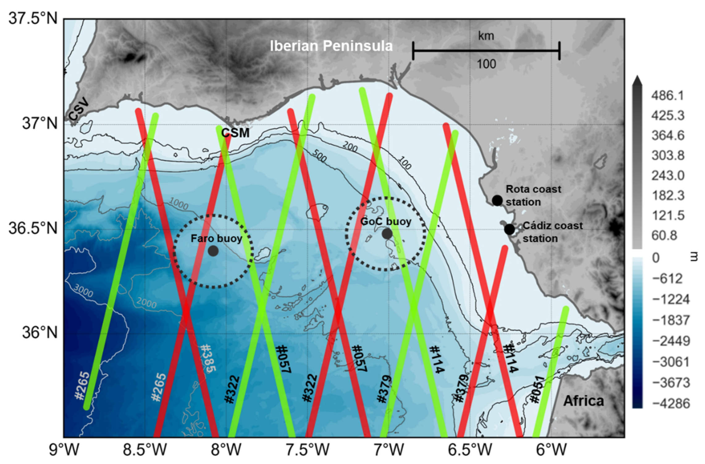
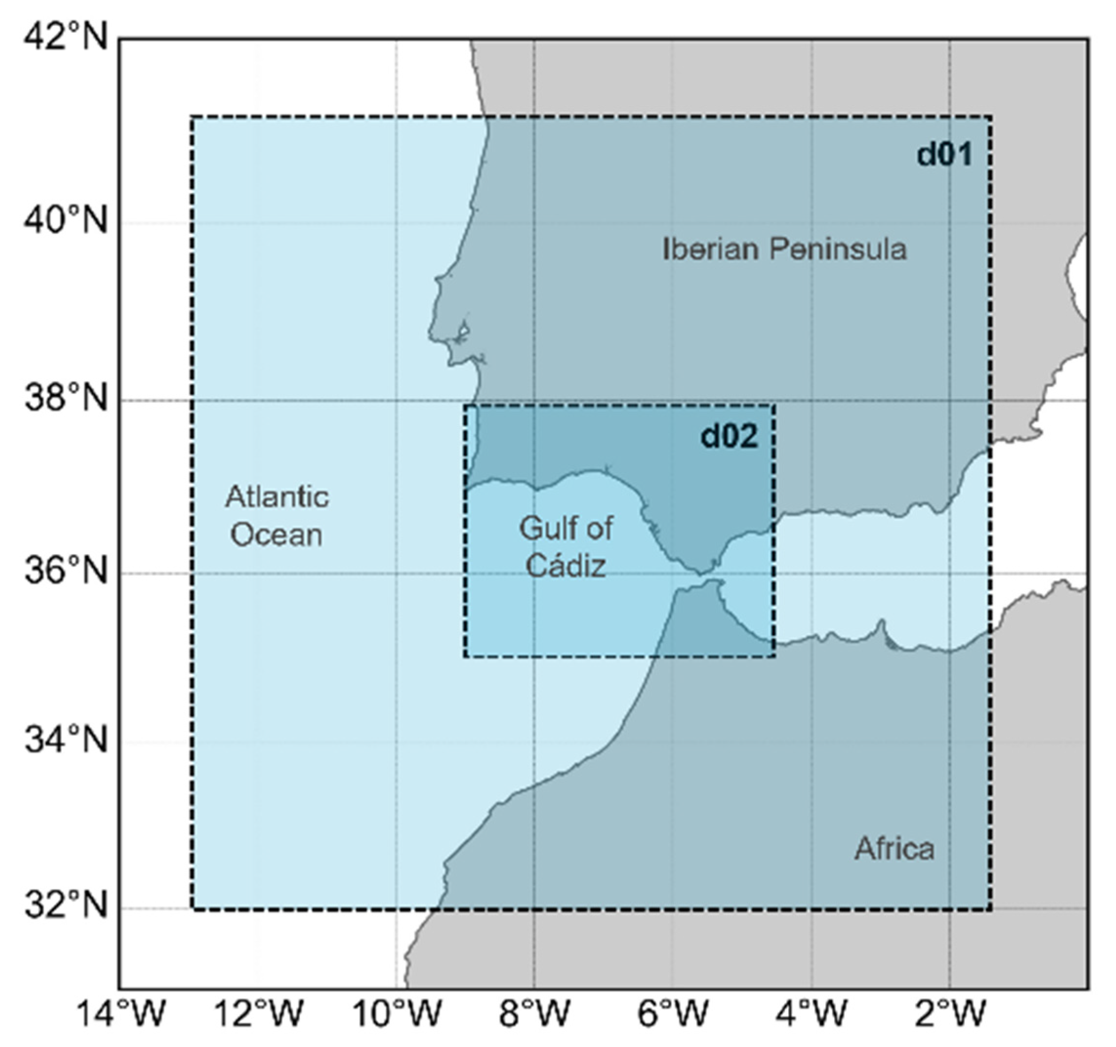
2.1. Study Area

The study area extends from Cape San Vicente (CSV) to the entrance of the Strait of Gibraltar (SG) (Figure 1), covering the Gulf of Cádiz (GoC), southern Spain. This area is characterised by abrupt changes in the orientation of the coastline, very complex coastal topography, and links between two basins with different characteristics. Such features favour the existence of a heterogeneous wind field, with topography-induced atmospheric flows [24] that strongly control the zonal sea surface circulation [25,26] and therefore, modulate variables of interest, such as sea surface temperature (SST) and chlorophyll concentration [27]. Such sea surface circulation over the continental shelf alternates westward/eastward modes, the former characterised by a coastal countercurrent, and the latter for inducing cold water upwellings along the coast [6,28]. Moreover, due to differences in the surface temperatures of the land and the sea, the coastal area of the GoC, is characterised by a land–sea breeze circulation, which is generally perpendicular to the coastline and can be extended up to 200 km inland [29]. Apart from the local geographic characteristics, the wind field in the area is also controlled by the large scale. Different studies demonstrated that the North Atlantic oscillation (NAO) is significantly related to the wind field in the area through the modulation of the Azores anticyclone [30,31]. The zonal component of the SSW is the most important meteorological agent affecting the ocean circulation in the area. Its variability is directly related to the sea surface circulation over the GoC [6], but also to the across shore sea level variability of the strait, contributing to the modulation of the water exchange through it, as observed from modelling studies [32], in situ [33], and altimeter data [34].

2.2. Altimetry Data

The along-track WS data from altimetry are retrieved from the retracking of the altimeter waveforms. The satellites have a repeat cycle of 27 days. The radar instrument, synthetic aperture radar altimeter (SRAL), has two measurement modes: low resolution (LRM) and SAR, the latter being the high-resolution along-track mode commonly used over the global ocean. Furthermore, the S3A/B SRAL generates level-2 data at 1 Hz and 20 Hz of the Ku and C bands (for more details see Sentinel-3 Altimetry Document Library at https://sentinel.esa.int/web/sentinel, accessed on 1 January 2022). The S3A/B level 2 data used were provided by the ESA Earth Console Parallel Processing Service (P-PRO) SAR versatile altimetric toolkit for ocean research and exploitation (SARvatore) service (https://ui-ppro.earthconsole.eu/, accessed on 1 January 2022), applying the pre-defined processing setup for coastal zones. The SAR Altimetry MOde Studies and Applications (SAMOSA++) model (Dinardo et al., 2020) is used in the retracking process and the final product is posted at 20 Hz, which results in ~330 m along-track spatial resolution measurements. Along-track WS data come from 12 S3A/B tracks over the GoC, detailed in

Table 1. Sentinel-3 A/B data availability (number of cycles, relative orbits and orientation) for the different comparisons among the datasets (the orientation of the different tracks is presented as ascending (A) or descending (D)).

Sentinel 3A				Sentinel 3B
Relative Orbit	N° Cycles S3A vs. WRF	N° Cycles S3A vs. Buoy	Orientation	Relative Orbit	N° Cycles S3B vs. WRF	N° Cycles S3B vs. Buoy	Orientation
#057	13	-	A	#051	14	-	D
#114	13	-	A	#057	14	26	A
#265	14	33	D	#114	14	29	A
#322	14	53	D	#265	13	-	D
#379	14	-	D	#322	13	-	D
#385	14	34	A	#379	13	-	D
Analysed period	From January 2020 to December 2020	From January 2017 to December 2020			From January 2020 to December 2020	From November 2018 to December 2020

. For the validation of the altimetry WS data with in situ measurements from the GoC buoy, only S3A/B data in a radius of 25 km around the position of the buoy were used, so the altimetry data can be considered co-located with the in situ data [18]. Only data from relative orbits #265, #322, #385 from S3A, and #057 and #114 from S3B satisfy the 25 km radius criteria (see Figure 1). Raw 20-Hz along-track WS data were edited eliminating the first 5 km of data closer to the coast, since demonstrated by [35], S3-SRAL altimeters start to give accurate data 5 km from the coast, due to coastal and land reflections that might contaminate the radar waveforms, making the retrieval of estimates of the derived geophysical parameters less accurate [36]. Furthermore, the methods presented in [37] were applied, in order to remove outliers and filter out noise signals. The aforementioned editing methodology consists of removing values larger than three times the standard deviation and replacing them with linearly interpolated values; this processing was applied in a 10-times loop [37,38].

2.3. In Situ Data

The in situ coastal wind data were extracted from four sources; (i) hourly time series of 10 m height WS and direction (WD), recorded by the weather station deployed by the Spanish Meteorology Agency (AEMET) in the city of Cádiz, (Cádiz coast station, Figure 1); (ii) same as (i), but located in Rota, (Rota coast station, Figure 1); (iii) in situ offshore wind data collected by two moored multi-instrument buoys. These buoys (GoC buoy and Faro buoy, Figure 1) provide an hourly time series of 3 m height WS and WD and are operated and maintained by the Spanish Port Authorities and the Hydrographic Institute of Portugal, respectively. The hourly data, distributed for public use, are built from averaging 10 min of raw data each hour. It is worth noting that these averages, related to spatially smoother wind fields (removing, for instance, small-scale variability due to eddies), should match better with the S3A/B data, which are averaged over the track segment inside the circular area with a radius of 25 km. Considering that the buoy registers wind parameters at 3 m over the surface, it is necessary to extrapolate the buoy data to a 10 m height wind speed, so it can be compared with altimetry derived WS data. For this purpose, the typically accepted logarithmic wind profile method [39,40,41] was applied to extrapolate the measured winds by the buoy from 3 to 10 m over the sea. Although there are several methods and variations used for this purpose, e.g., stress equivalent winds [42] that consider the air mass density and stability, for practical reasons, here we used the logarithmic wind profile method, which is suitable for our aim, requiring only WS and WD measurements and proven to be consistent over the first 30 m of sea surface [43,44].

2.4. Weather Research and Forecasting Model Data

Model data were obtained using the mesoscale, non-hydrostatic WRF model version 4.2 [22]. The model was used to produce dynamically downscaled hourly 10 m WS and WD over the complete study area during 2020, with a temporal resolution of 1 h and 3 km grid (d02). The d02 domain was one-way nested within a parent domain of 9 km grid (d01), as depicted in Figure 2, in order to allow communication from the parent (lower resolution) to the child domain (higher resolution), but not vice versa.

The initial and boundary conditions were supplied by the NCEP/NCAR operational Global Forecast System (GFS) with 0.25° of spatial resolution and 6 h of temporal sampling (National Centers for Environmental Prediction/National Weather Service/NOAA/US Department of Commerce, 2015). Boundary conditions were applied to the parent domain (d01). The dynamical setup of the simulation was based on the optimised design presented by [45] after performing 4150 daily simulations over southern Spain (

Table 2. Configuration options selected for the WRF simulations, based on [45].

Scheme or Parameterization	Selected Option
Initialization	NCEP/NARC GFS 0.25°
Microphysics	SBU-Lin
Longwave radiaion	RRTMG
Shortwave radiation	Dudhia
Cumulus	Kain-Fritsch
Surface layer	MM5 similarity
Planetary boundary layer	YSU
Vertical levels number	36
Diffusion 6th order option	Knievel
Damping	Rayleigh
Topography model	GTOPO30
Land uses	GLC
Nudging	Grid nudging (d01)/Observational nudging (d02)
Sea surface temperature	Updated every 6 h

). Unlike previous studies in the area [40,44,45], which consider constant sea surface temperature (SST), in our study, the SST was updated every 6 h. Although the overall impact is expected to be small, it is a more realistic approach and might have an impact under specific conditions or in specific areas [46].

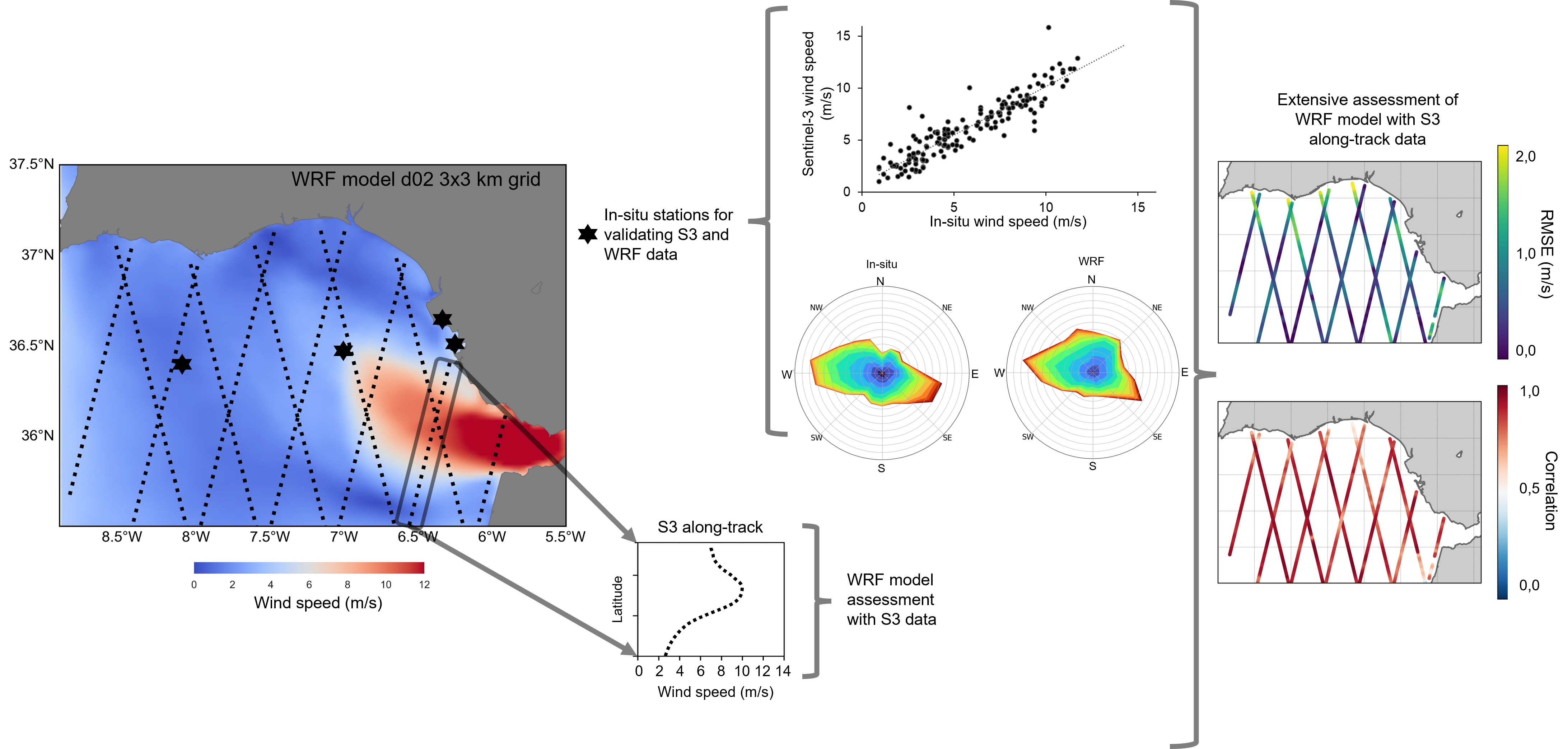
2.5. Assessment of Altimeter and Model Data

Prior to the comparisons, the WRF wind data were linearly interpolated to the position of in situ instruments, as well as to the S3A/B along-track measurement positions. Several statistical parameters were used to compare the wind speed and direction from the altimeter and model, according to previous studies [44,47,48]. Root mean square error (RMSE) (1), normalised root mean square error (NRMSE) (2), bias (3), and Pearson’s correlation coefficient (r) (4) were used to evaluate wind speed, while bias and standard deviation error (STDE) (5) were applied to the wind direction comparisons results.

$$RMSE=\sqrt{\frac{{\sum }_{i=1}^n{\left(P_i-O_i\right)}^2}{n}}$$

(1)

$$NRMSE=\frac{RMSE}{ma{x}_{i}O-mi{n}_{i}O}$$

(2)

$$bias=\frac{{\sum }_{i=1}^n\left(P_i-O_i\right)}{n}$$

(3)

$$r=\frac{{\sum }_{i=1}^n\left(O_i-\overline{O}\right)\left(P_i-\overline{P}\right)}{{\left[{\sum }_{i=1}^n{\left(O_i-\overline{O}\right)}^2{\sum }_{i=1}^n{\left(P_i-\overline{P}\right)}^2\right]}^{\raisebox{1ex}{$1$}\!\left/ \!\raisebox{-1ex}{$2$}\right.}}$$

(4)

$$STDE={\left[(RMS{E}^2-bia{s}^2)\right]}^{\frac{1}{2}}$$

(5)

where P represents the co-located WS or WD from the data source that is being evaluated (model: WS, WD, and altimetry: WS); O denotes the co-located WS or WD from the reference data source (in situ stations). Note that WD is an angular variable, therefore, to avoid errors related to 0° and 360° overlapping, WD bias and WD STDE were calculated for a new circular variable (d) (6), bounded between [−180, 180], and obtained from the observed (O) and predicted (P) wind directions as follows:

$$d_i=\{\begin{array}{c}{d}_i^p-d_i^o if \left|d_i^p-d_i^o\right|<180\\ d_i^p-d_i^o-360 if d_i^p-d_i^o>180\\ d_i^p-d_i^o+360 if d_i^p-d_i^o<-180\end{array}$$

(6)

3. Results and Discussion

3.1. Preliminary Validation of the Data Sources

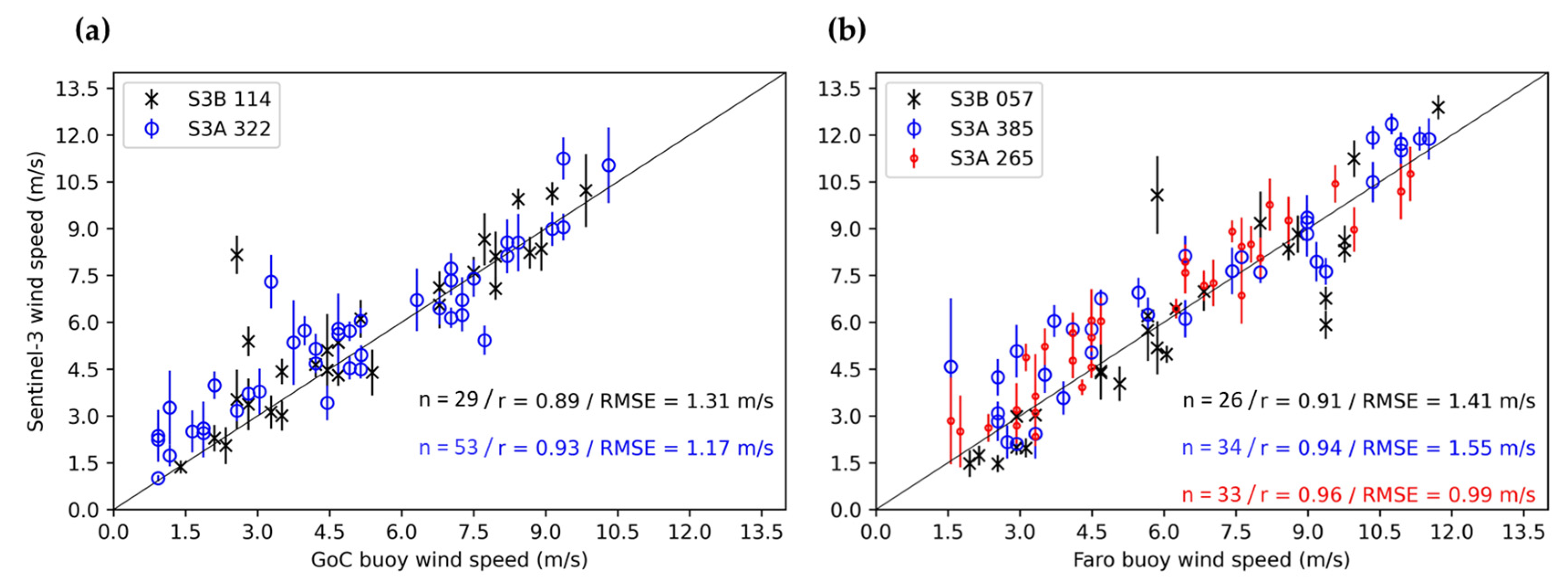
3.1.1. Altimetry Wind Speed Validation Using In Situ Data

All available WS data derived from altimetry and corresponding to relative orbits #265, #322, and #385 from S3A, as well as #057 and #114 from S3B that matched the 25 km radius criteria (presented in Section 2.2) from 6 January 2017 to 31 December 2020, were compared against the moored GoC buoy and the Faro buoy, using some of the statistical parameters presented in Section 2.4, to ensure the correct performance of the altimetry sensors over the area of interest. The results from the comparison are shown in Figure 3. The scatterplots present the GoC buoy (Figure 3a) and Faro buoy (Figure 3b) WS measurements against the average of all the S3A and S3B measurements within the 25-km radius around the buoys; the corresponding standard deviation threshold of each track segment is also shown. Due to the different starting points of S3A (since 2016) and S3B (since 2018), the number of available data for the latter is lower than that of S3A.

These results are in line with the reported accuracy in the S3 Wind and Waves Cyclic Performance Report for the period from December 2020 to January 2021 [20]. They are also in agreement with those reported by [18], who compared WS from S3A/B with more than 80 moored buoys. There is a strong linear relationship between the altimeters and the GoC buoy dataset according to the average r coefficients (0.94 for S3A and 0.90 for S3B, 99% of confidence level). As it was expected, the best results correspond with the relative orbits closer to the location of the buoys S3A #265.

The differences observed between the two data sources might be related with the representativeness of the spatio-temporal domains. Firstly, in the spatial domain, the in situ data represent a local estimate and therefore include the wind variability over all scales [49]. However, the radar altimeter considers the entire footprint [50]. Secondly, the time difference between the satellite passing over the buoy and the operating period of the in situ instrument; this difference was calculated to be 30 min maximum. This temporal difference could also explain the presence of outliers, since unlike the in situ data, the altimeter WS is estimated from instantaneous measurements of the sea surface state. An example is the outlier observed in the S3B #114 vs. GoC buoy scatterplot (Figure 3a), which affects the statistical scores and could compromise the comparisons. This mismatch represents a S3B WS value of 8.00 m/s against an in situ measurement of 2.50 m/s, approximately, and corresponds to 21:00 UTC in situ data and 21:26 UTC altimetry data of 25 November 2020. As depicted in Figure 4e, where hourly WS from the GoC buoy for that day is presented, WS was highly variable during the entire day, especially between 14:00 UTC and 23:00 UTC, with WS ranging from 2.00 m/s to 11.50 m/s. Sentinel-3B passed over the GoC buoy position at 21:26 UTC and detected high variability in the spatial domain, as shown in Figure 4a. The radargram of the power waveforms for S3B relative orbit #144 in the vicinity of the buoy is shown in Figure 4c, together with the along-track WS (Figure 4a) and the along-track backscattering coefficient (σ0) (Figure 4b). Note that only the power from gates 320 to 365 are shown in the radargram; moreover, since the product used to generate this radargram is not yet corrected by the retracking process, a leading edge deviation over latitude 36.30°N is observed. Regarding the power represented in the radargram (Figure 4c), a fall is clearly observed in the segment between latitudes 35.80°N and 36.25°N. The strong decrease in power affects the retracking of the waveforms and, therefore, the retrieval of the geophysical parameters, as shown in [35]. The retracking of these waveforms results in a strong decrease in the retrieved σ0 and therefore, a rise in the derived along-track WS. This may be related to the existence of a strong and sporadic wind gust, which would agree with the high spatio-temporal variability observed during the day by the in situ sensor. Wind gusts can exceed 20 m/s over the area [51], also dramatically increasing the roughness of the sea surface. If the satellite crosses the area affected by the wind gust, a decrease in the returning signal received by the altimeter should be observed. However, this cannot be confirmed by the buoy data due to its sampling time (measurement recorded 26 min before the satellite pass).

3.1.2. WRF Model Wind Velocity Validation against In Situ Data

In this section, hourly WS and WD data for 2020, obtained from the WRF model simulations, are compared to in situ data from the Cádiz and Rota coast meteorological stations and the GoC and Faro buoys to ensure that the model performance over the study area is adequate. The wind rose diagrams representing the WD and WD data used to estimate the statistical parameters represented in

Table 3. Statistical scores from the comparison among in situ data from the different stations and buoys against simulations from the WRF model.

	Wind Speed				Wind Direction
In Situ Station	Bias (m/s)	RMSE (m/s)	NRMSE (m/s)	r	Bias (°)	STDE (°)
GoC buoy	0.74	1.93	0.12	0.80	6.74	47.10
Cádiz coast station	−0.13	1.74	0.12	0.74	5.78	54.49
Rota coast station	0.44	1.65	0.16	0.74	8.35	48.68
Faro buoy	0.33	1.59	0.10	0.85	5.54	33.84

are shown in Figure 5, where the predominant zonal component of the wind over the area can be observed. The four figures depict the high variability of the wind over the study area. The resulting scores, shown in Table 3, demonstrate the overall good performance of the dynamical setup applied to the model, which are in line with similar studies [40,44] usually performed only for open ocean comparisons. However, the model overestimates/underestimates the WS at the Faro and GoC buoy and Rota coast station/Cádiz coast station positions, respectively, as indicated for the bias scores in Table 3. Although there are differences among WS RMSE from the three stations, once the parameter is normalised (NRMSE) using the range of variation in the WS, these differences are reduced. The best results are obtained for the Faro buoy site, which is the farthest location from the coast.

3.2. WRF Model Spatial Assessment Using Altimetry Data

In this section, the innovative use of altimetry WS for the spatial evaluation of WS from the WRF model over the study area is carried out through quantitative comparisons using WS retrievals from S3A and S3B altimeters. Special focus is on the coastal fringe, where other sensors, such as the scatterometers, cannot provide useful data for validating the model. The statistical results from the evaluation of WS data from the WRF model simulations with WS from the S3A/B tracks over the study area are presented here. In order to assess the accuracy of the WRF WS spatial variability, model outputs were linearly interpolated over the positions of the satellite track measurements for 2020. As depicted in Figure 6a,b, the averaged WS spatial variability obtained from both altimetry (Figure 6a) and the WRF model (Figure 6b) matches for almost the whole study area. This agreement between the WRF model and the S3A/B WS data for the set of tracks used is confirmed by the r Pearson’s values, which are mostly over 0.80, being the average correlation value for all the tracks 0.85 (confidence level: 99%, Figure 6c). The RMSE (Figure 6d) is small for all tracks, frequently below 1.0 m/s (average RMSE: 0.65 m/s). Lower correlations and larger RMSEs are generally found near the coastal fringe. In the sector [5–20 km] from land, the averages of the statistical parameters are r = 0.79 and RMSE 0.88 m/s, which is also evident in the WS average maps, since altimetry WS is slightly lower over the coastal area than the WS from WRF. Considering that the altimetry data over the 5 km closest to land were removed, the decrease in the statistical scores from the comparison adjacent to the coast is not due to the land contamination of the altimetry signal, but rather to the WRF simulations. The model WS overestimation in coastal areas is an issue previously described by different authors [39,52,53] and is most likely caused by the high spatial variability of the wind field over these areas due to the thermal atmospheric gradients [3], which may not be properly reproduced by the WRF model at fine scales. Such misrepresentation could be related to the lack of information and crude representation of the land surface that can considerably affect the simulation of the fluxes driving the associated boundary layer processes [54]. Although satellite tracks do not cover the entire WRF domain area, the results prove that using along-track WS from altimetry enables the estimation of the correlation coefficient and RMSE spatial maps for the area, which facilitate the assessment of the WRF model performance over the study area. Moreover, the presence of altimetry data up to 5 km from land allows the detection of weaknesses in the model performance over the complex land–sea transition fringe.

3.3. Observability of Spatial Variability

The wind field over the GoC is characterised by its high spatial variability and high-intensity events. In this section, a qualitative comparison of the spatial variability of the WS reproduced by the WRF model with the S3A/B data is presented to investigate the capabilities of using altimetry data for assessing the WRF model under complex conditions. For this purpose, WS from three S3A/B tracks under different atmospheric situations are compared with the wind field obtained from the corresponding WRF model simulations. The comparisons are shown in Figure 7. Figure 7a depicts the simulated wind field on 31 December 2020 at 11:00 UTC. The satellite crossed the area at 10:35 UTC. A weak northerly wind dominated over the whole GoC. The along-track spatial variability observed from the altimeter measurements agrees with the outputs of the WRF model, especially for the northernmost part of the track, stating the good performance of the WRF model even at the positions closer to the coast.

During the satellite pass on 25 June 2020 at 21:32 UTC the wind field reproduced by the model at 22:00 UTC (Figure 7b) over the GoC can be divided into two sectors: the westernmost area is dominated by mid intensity northwesterlies, while in the sector to the east, the wind is weaker and from west. Furthermore, as also shown by the along-track S3A WS, the intensity increases further from the coast from 6 to 10–12 m/s. Such spatial variability of the WS is well represented by both data sets; however, close to the coast, the differences among the altimeter derived WS and the WRF model output increase. Such disagreement may be caused by two factors as previously mentioned in Section 3.1: the time difference between the satellite pass and the model simulation; and the precision of the WRF model at fine scales close to the complex land–sea boundary. Such discrepancies in the WRF model can be detected thanks to the presence of altimetry data in the coastal fringe.

Finally, Figure 7c shows an example of dominant easterlies over the GoC, as simulated by the WRF for 21 February 2020 at 11:00 UTC. S3B crossed the area at 10:37 UTC. WRF output displays a heterogeneous wind field over the area, with a remarkable easterly jet coming from the Strait of Gibraltar and a generalised decrease towards the northern coast. However, over 36.8° latitude, a slight underestimation from the WRF model is observed, which coincides with the area covered by the Guadalquivir River mouth, an area characterised by high contrasts and variability.

4. Conclusions

This study presents the quality and capabilities of WS from satellite altimetry for the spatial assessment of WS outputs from the WRF model over the complex area of the GoC. In order to achieve this, three WS data sources were compared: in situ measurements, S3A/B satellite altimetry derived measurements at 20 Hz, and the WRF model simulations from a nested domain of 3 km grid and 1 h temporal resolution. From the results of the different comparisons, we conclude that the quality of the high-resolution (20 Hz) S3A/B WS data satisfies the general mission requirements over the study area, and even though the GoC buoy is located in a complex area affected by coastal-related processes, the results are in line with previous studies focused on the open ocean. Regarding the validation of the WRF model against in situ data, the simulations of the surface WS over the area are of good quality; this confirms the goodness of the dynamical parameterisations proposed by [45]. Note that we introduced a modification in the configuration by updating the SST every 6 h instead of maintaining a constant value, which makes the setup more realistic. The spatial variability of the WS derived from the model was compared to along-track altimetry-derived WS data. This comparison, and considering the complex characteristics of the analysed region, exhibits the potential of the altimetry data for the spatial evaluation of numerical models. In this case, the altimetry data enable the detection of a certain level of degradation of the WRF outcomes near the coastal fringe, which is in line with previously detected WS overestimation of the WRF model in coastal areas, which supports the need to conduct further analyses into the dynamical phenomena and the effect of using a more accurate surface representation. It is important to note that these model deficiencies in the coastal band are detected thanks to the presence of altimetry data up to 5 km from the land, enabling the fine tuning and evaluation of NWP models over the complex coastal fringe. Qualitatively, we proved the agreement between altimetry and WRF model data sets under low/high wind speed conditions. However, it is important to note the limitations related to altimetry, as it is not possible to obtain the wind direction. Furthermore, altimetry data are instantaneous and events of time scales shorter than the time resolution of the model may lead to mismatches. Moreover, perpendicular to the track, the altimeters do not measure the variability in scales smaller than the across track footprint length. In this sense, it is important to highlight the need for the continuous improvement of satellite altimetry and model outputs in the coastal fringe in order to obtain realistic geophysical parameters in these areas. Present and future satellite altimetry missions will allow the exploitation of fully focused SAR data for a better characterisation of ocean processes in the 0–5 km coastal band. This study proves the high quality of Sentinel-3A/B WS retrievals over complex areas, and aims to foster the use of this data for the improvement of knowledge of WS and sea surface circulation over areas where the availability of in situ measurements is limited or inexistent. We showed how the spatial coverage of satellite altimetry enables the spatial assessment of high-resolution NWP models in water-covered surfaces, including coastal areas up to 5 km from land, a feature that sets altimetry as a complementary data source to improve the study and prediction of the wind in coastal areas together with some of the current systems, such as scatterometers, high frequency radars, and SAR wind fields.

References

1. Kelly, K.A.; Dickinson, S.; Yu, Z. NSCAT Tropical Wind Stress Maps: Implications for Improving Ocean Modeling. J. Geophys. Res. Ocean. 1999, 104, 11291–11310. [Google Scholar] [CrossRef]
2. GCOS. The Global Observing System for Climate Implementation Needs. World Meteorol. Organ. 2016, 200, 316. [Google Scholar]
3. Cerralbo, P.; Grifoll, M.; Moré, J.; Bravo, M.; Sairouní Afif, A.; Espino, M. Wind Variability in a Coastal Area (Alfacs Bay, Ebro River Delta). Adv. Sci. Res. 2015, 12, 11–21. [Google Scholar] [CrossRef]
4. Lu, Y.; Zhang, B.; Perrie, W.; Mouche, A.; Li, X.; Wang, H. A C-Band Geophysical Model Function for Determining Coastal Wind Speed Using Synthetic Aperture Radar. Prog. Electromagn. Res. Symp. 2018, 11, 2417–2428. [Google Scholar] [CrossRef]
5. Bôas, A.B.V.; Ardhuin, F.; Ayet, A.; Bourassa, M.A.; Brandt, P.; Chapron, B.; Cornuelle, B.D.; Farrar, J.T.; Fewings, M.R.; Fox-Kemper, B.; et al. Integrated Observations of Global Surface Winds, Currents, and Waves: Requirements and Challenges for the next Decade. Front. Mar. Sci. 2019, 6, 1–34. [Google Scholar] [CrossRef]
6. Mulero-Martínez, R.; Gómez-Enri, J.; Mañanes, R.; Bruno, M. Assessment of Near-Shore Currents from CryoSat-2 Satellite in the Gulf of Cádiz Using HF Radar-Derived Current Observations. Remote Sens. Environ. 2021, 256, 112310. [Google Scholar] [CrossRef]
7. Rio, M.H.; Mulet, S.; Picot, N. Beyond GOCE for the Ocean Circulation Estimate: Synergetic Use of Altimetry, Gravimetry, and in Situ Data Provides New Insight into Geostrophic and Ekman Currents. Geophys. Res. Lett. 2014, 41, 8918–8925. [Google Scholar] [CrossRef]
8. Mears, C.A.; Scott, J.; Wentz, F.J.; Ricciardulli, L.; Leidner, S.M.; Hoffman, R.; Atlas, R. A Near-Real-Time Version of the Cross-Calibrated Multiplatform (CCMP) Ocean Surface Wind Velocity Data Set. J. Geophys. Res. Ocean. 2019, 124, 6997–7010. [Google Scholar] [CrossRef]
9. Astudillo, O.; Dewitte, B.; Mallet, M.; Frappart, F.; Rutllant, J.A.; Ramos, M.; Bravo, L.; Goubanova, K.; Illig, S. Surface Winds off Peru-Chile: Observing Closer to the Coast from Radar Altimetry. Remote Sens. Environ. 2017, 191, 179–196. [Google Scholar] [CrossRef]
10. Vogelzang, J.; Stoffelen, A.; Lindsley, R.D.; Verhoef, A.; Verspeek, J. The ASCAT 6.25-Km Wind Product. IEEE J. Sel. Top. Appl. Earth Obs. Remote Sens. 2017, 10, 2321–2331. [Google Scholar] [CrossRef]
11. Carvalho, D.; Rocha, A.; Gómez-Gesteira, M.; Silva Santos, C. Offshore Winds and Wind Energy Production Estimates Derived from ASCAT, OSCAT, Numerical Weather Prediction Models and Buoys—A Comparative Study for the Iberian Peninsula Atlantic Coast. Renew. Energy 2017, 102, 433–444. [Google Scholar] [CrossRef]
12. Korsbakken, E.; Johannessen, J.A.; Johannessen, O.M. Coastal Wind Field Retrievals from ERS SAR Images. In Proceedings of the IGARSS’97. 1997 IEEE International Geoscience and Remote Sensing Symposium Proceedings. Remote Sensing-A Scientific Vision for Sustainable Development, Singapore, 3–8 August 1997; Volume 103, pp. 1211–1216. [Google Scholar] [CrossRef]
13. Zhou, L.; Zheng, G.; Li, X.; Yang, J.; Ren, L.; Chen, P.; Zhang, H.; Lou, X. An Improved Local Gradient Method for Sea Surface Wind Direction Retrieval from SAR Imagery. Remote Sens. 2017, 9, 671. [Google Scholar] [CrossRef]
14. Mu, S.; Li, X.; Wang, H. The Fusion of Physical, Textural, and Morphological Information in SAR Imagery for Hurricane Wind Speed Retrieval Based on Deep Learning. IEEE Trans. Geosci. Remote Sens. 2022, 60, 1–13. [Google Scholar] [CrossRef]
15. Sar, S.C.; Yu, P.; Xu, W.; Zhong, X.; Johannessen, J.A.; Yan, X.; Geng, X.; He, Y.; Lu, W. A Neural Network Method for Retrieving Sea Surface Wind Speed for C-Band SAR. Remote Sens. 2022, 14, 2269. [Google Scholar]
16. Abdalla, S. Ku-Band Radar Altimeter Surface Wind Speed Algorithm. Mar. Geod. 2012, 35, 276–298. [Google Scholar] [CrossRef]
17. Witter, D.L.; Chelton, D.B. A Geosat Altimeter Wind Speed Algorithm and a Method for Altimeter Wind Speed Algorithm Development. J. Geophys. Res. 1991, 96, 8853–8860. [Google Scholar] [CrossRef]
18. Yang, J.; Zhang, J.; Jia, Y.; Fan, C.; Cui, W. Validation of Sentinel-3A/3B and Jason-3 Altimeter Wind Speeds and Significant Wave Heights Using Buoy and ASCAT Data. Remote Sens. 2020, 12, 2079. [Google Scholar] [CrossRef]
19. Quartly, G.D.; Nencioli, F.; Raynal, M.; Bonnefond, P.; Garcia, P.N.; Garcia-Mondéjar, A.; de la Cruz, A.F.; Cretaux, J.F.; Taburet, N.; Frery, M.L.; et al. The Roles of the S3MPC: Monitoring, Validation and Evolution of Sentinel-3 Altimetry Observations. Remote Sens. 2020, 12, 1763. [Google Scholar] [CrossRef]
20. Abdalla, S.; Centre (MPC) for the Copernicus. Sentinel-3 Mission S3 Wind and Waves Cyclic Performance Report; Cycle No. 066-A End Date: 31 December 2020 Cycle No. 047-B; European Space Agency: Paris, France, 2021. [Google Scholar]
21. Powers, J.G.; Klemp, J.B.; Skamarock, W.C.; Davis, C.A.; Dudhia, J.; Gill, D.O.; Coen, J.L.; Gochis, D.J.; Ahmadov, R.; Peckham, S.E.; et al. The Weather Research and Forecasting Model: Overview, System Efforts, and Future Directions. Bull. Am. Meteorol. Soc. 2017, 98, 1717–1737. [Google Scholar] [CrossRef]
22. Skamarock, W.C.; Klemp, J.B.; Dudhia, J.; Gill, D.O.; Zhiquan, L.; Berner, J.; Wang, W.; Powers, J.G.; Duda, M.G.; Barker, D.M.; et al. A Description of the Advanced Research WRF Model Version 4; National Center for Atmospheric Research: Boulder, CO, USA, 2019; Volume 145, p. 145. [Google Scholar]
23. Bhowmick, S.A.; Modi, R.; Sandhya, K.G.; Seemanth, M.; Balakrishnan Nair, T.M.; Kumar, R.; Sharma, R. Analysis of SARAL/AltiKa Wind and Wave over Indian Ocean and Its Real-Time Application in Wave Forecasting System at ISRO. Mar. Geod. 2015, 38, 396–408. [Google Scholar] [CrossRef]
24. Carvalho, D.; Rocha, A.; Gómez-Gesteira, M.; Silva Santos, C. Sensitivity of the WRF Model Wind Simulation and Wind Energy Production Estimates to Planetary Boundary Layer Parameterizations for Onshore and Offshore Areas in the Iberian Peninsula. Appl. Energy 2014, 135, 234–246. [Google Scholar] [CrossRef]
25. Peliz, A.; Dubert, J.; Marchesiello, P.; Teles-Machado, A. Surface Circulation in the Gulf of Cadiz: Model and Mean Flow Structure. J. Geophys. Res. Ocean. 2007, 112, C11015. [Google Scholar] [CrossRef]
26. Navarro, G.; Escudier, R.; Pascual, A.; Caballero, I.; Vázquez, A. Singular Value Decomposition of Ocean Surface Chlorophyll and Sea Level Anomalies in the Gulf of Cadiz (South-Western Iberian Peninsula). In Proceedings of the 20 Years of Progress in Radar Altimetry Conference, Venice, Italy, 24–29 September 2012. [Google Scholar]
27. Garel, E.; Laiz, I.; Drago, T.; Relvas, P. Characterisation of Coastal Counter-Currents on the Inner Shelf of the Gulf of Cadiz. J. Mar. Syst. 2016, 155, 19–34. [Google Scholar] [CrossRef]
28. Hernández-Ceballos, M.A.; Adame, J.A.; Bolívar, J.P.; De la Morena, B.A. A Mesoscale Simulation of Coastal Circulation in the Guadalquivir Valley (Southwestern Iberian Peninsula) Using the WRF-ARW Model. Atmos. Res. 2013, 124, 1–20. [Google Scholar] [CrossRef]
29. Folkard, A.M.; Davies, P.A.; Fiúza, A.F.G.; Ambar, I. Remotely Sensed Sea Surface Thermal Patterns in the Gulf Of-Cadiz and the Strait of Gibraltar: Variability, Correlations, and Relationships with the Surface Wind Field. J. Geophys. Res. Ocean. 1997, 102, 5669–5683. [Google Scholar] [CrossRef]
30. Hidalgo, P.; Gallego, D. A Historical Climatology of the Easterly Winds in the Strait of Gibraltar. Atmosfera 2019, 32, 181–195. [Google Scholar] [CrossRef]
31. Brandt, P.; Rubino, A.; Sein, D.V.; Baschek, B.; Izquierdo, A.; Backhaus, J.O. Sea Level Variations in the Western Mediterranean Studied by a Numerical Tidal Model of the Strait of Gibraltar. J. Phys. Oceanogr. 2004, 34, 433–443. [Google Scholar] [CrossRef]
32. Ross, T.; Garrett, C.; Traon, P.Y. Le Western Mediterranean Sea-Level Rise: Changing Exchange Flow through the Strait of Gibraltar. Geophys. Res. Lett. 2000, 27, 2949–2952. [Google Scholar] [CrossRef]
33. Gómez-Enri, J.; González, C.J.; Passaro, M.; Vignudelli, S.; Álvarez, O.; Cipollini, P.; Mañanes, R.; Bruno, M.; López-Carmona, M.P.; Izquierdo, A. Wind-Induced Cross-Strait Sea Level Variability in the Strait of Gibraltar from Coastal Altimetry and in-Situ Measurements. Remote Sens. Environ. 2019, 221, 596–608. [Google Scholar] [CrossRef]
34. Aldarias, A.; Gomez-Enri, J.; Laiz, I.; Tejedor, B.; Vignudelli, S.; Cipollini, P. Validation of Sentinel-3A SRAL Coastal Sea Level Data at High Posting Rate: 80 Hz. IEEE Trans. Geosci. Remote Sens. 2020, 58, 3809–3821. [Google Scholar] [CrossRef]
35. Gómez-Enri, J.; Vignudelli, S.; Cipollini, P.; Coca, J.; González, C.J. Validation of CryoSat-2 SIRAL Sea Level Data in the Eastern Continental Shelf of the Gulf of Cadiz (Spain). Adv. Space Res. 2018, 62, 1405–1420. [Google Scholar] [CrossRef]
36. Bouffard, J.; Pascual, A.; Ruiz, S.; Faugère, Y.; Tintoré, J. Coastal and Mesoscale Dynamics Characterization Using Altimetry and Gliders: A Case Study in the Balearic Sea. J. Geophys. Res. Ocean. 2010, 115, 1–17. [Google Scholar] [CrossRef]
37. Meloni, M.; Bouffard, J.; Doglioli, A.M.; Petrenko, A.A.; Valladeau, G. Toward Science-Oriented Validations of Coastal Altimetry: Application to the Ligurian Sea. Remote Sens. Environ. 2019, 224, 275–288. [Google Scholar] [CrossRef]
38. Paulson, C.A. The Mathematical Representation of Wind Speed and Temperature Profiles in the Unstable Atmospheric Surface Layer. J. Appl. Meteorol. 1970, 9, 857–861. [Google Scholar] [CrossRef]
39. Powell, M.D.; Vickery, P.J.; Reinhold, T.A. Reduced Drag Coefficient for High Wind Speeds in Tropical Cyclones. Nature 2003, 422, 279–283. [Google Scholar] [CrossRef]
40. Carvalho, D.; Rocha, A.; Gómez-Gesteira, M.; Santos, C. A Sensitivity Study of the WRF Model in Wind Simulation for an Area of High Wind Energy. Environ. Model. Softw. 2012, 33, 23–34. [Google Scholar] [CrossRef]
41. De Kloe, J.; Stoffelen, A.; Verhoef, A. Improved Use of Scatterometer Measurements by Using Stress-Equivalent Reference Winds. IEEE J. Sel. Top. Appl. Earth Obs. Remote Sens. 2017, 10, 2340–2347. [Google Scholar] [CrossRef]
42. Emeis, S.; Turk, M. Comparison of Logarithmic Wind Profiles and Power Law Wind Profiles and Their Applicability for Offshore Wind Profiles. In Wind Energy; Springer: Berlin/Heidelberg, Germany, 2007; pp. 61–64. [Google Scholar] [CrossRef]
43. Peña, A.; Gryning, S.E.; Hasager, C.B. Measurements and Modelling of the Wind Speed Profile in the Marine Atmospheric Boundary Layer. Bound.-Layer Meteorol. 2008, 129, 479–495. [Google Scholar] [CrossRef]
44. Arasa, R.; Porras, I.; Domingo-Dalmau, A.; Picanyol, M.; Codina, B.; González, M.Á.; Piñón, J. Defining a Standard Methodology to Obtain Optimum WRF Configuration for Operational Forecast: Application over the Port of Huelva (Southern Spain). Atmos. Clim. Sci. 2016, 6, 329–350. [Google Scholar] [CrossRef]
45. Salvação, N.; Guedes Soares, C. Wind Resource Assessment Offshore the Atlantic Iberian Coast with the WRF Model. Energy 2018, 145, 276–287. [Google Scholar] [CrossRef]
46. Li, H.; Claremar, B.; Wu, L.; Hallgren, C.; Körnich, H.; Ivanell, S.; Sahlée, E. A Sensitivity Study of the WRF Model in Offshore Wind Modeling over the Baltic Sea. Geosci. Front. 2021, 12, 101229. [Google Scholar] [CrossRef]
47. Marta-Almeida, M.; Teixeira, J.C.; Carvalho, M.J.; Melo-Gonçalves, P.; Rocha, A.M. High Resolution WRF Climatic Simulations for the Iberian Peninsula: Model Validation. Phys. Chem. Earth Parts A/B/C 2016, 94, 94–105. [Google Scholar] [CrossRef]
48. Carvalho, D.; Rocha, A.; Gómez-Gesteira, M. Ocean Surface Wind Simulation Forced by Different Reanalyses: Comparison with Observed Data along the Iberian Peninsula Coast. Ocean Model. 2012, 56, 31–42. [Google Scholar] [CrossRef]
49. Stoffelen, A. Toward the True Near-Surface Wind Speed: Error Modeling and Calibration Using Triple Collocation. J. Geophys. Res. Ocean. 1998, 103, 7755–7766. [Google Scholar] [CrossRef]
50. Passaro, M.; Cipollini, P.; Vignudelli, S.; Quartly, G.D.; Snaith, H.M. ALES: A Multi-Mission Adaptive Subwaveform Retracker for Coastal and Open Ocean Altimetry. Remote Sens. Environ. 2014, 145, 173–189. [Google Scholar] [CrossRef]
51. Adame, J.A.; Lope, L.; Hidalgo, P.J.; Sorribas, M.; Gutiérrez-Álvarez, I.; del Águila, A.; Saiz-Lopez, A.; Yela, M. Study of the Exceptional Meteorological Conditions, Trace Gases and Particulate Matter Measured during the 2017 Forest Fire in Doñana Natural Park, Spain. Sci. Total Environ. 2018, 645, 710–720. [Google Scholar] [CrossRef]
52. Ngan, F.; Kim, H.; Lee, P.; Al-Wali, K.; Dornblaser, B. A Study of Nocturnal Surface Wind Speed Overprediction by the WRF-ARW Model in Southeastern Texas. J. Appl. Meteorol. Climatol. 2013, 52, 2638–2653. [Google Scholar] [CrossRef]
53. Misaki, T.; Ohsawa, T.; Konagaya, M.; Shimada, S.; Takeyama, Y.; Nakamura, S. Accuracy Comparison of Coastal Wind Speeds between WRF Simulations Using Different Input Datasets in Japan. Energies 2019, 12, 2754. [Google Scholar] [CrossRef]
54. Román-Cascón, C.; Lothon, M.; Lohou, F.; Hartogensis, O.; Vila-Guerau De Arellano, J.; Pino, D.; Yagüe, C.; Pardyjak, E.R. Surface Representation Impacts on Turbulent Heat Fluxes in the Weather Research and Forecasting (WRF) Model (v.4.1.3). Geosci. Model Dev. 2021, 14, 3939–3967. [Google Scholar] [CrossRef]
Figure 1. Study area (Gulf of Cádiz, southwestern coast of the Iberian Peninsula) along with the spatial distribution of the data sources used in this work and some geographical features: S3A tracks (red line), S3B tracks (green line), location of the moored (GoC buoy and Faro buoy) along with the 25 km radius area used to select S3A/B data for its validation (dotted contoured area), location of the land-based meteorological stations from the Spanish Meteorological Office (Cádiz coast station and Rota coast station), Cape Santa Maria (CSM), and Cape San Vicente (CSV).
Remotesensing 14 04036 g001
Figure 2. WRF model domains d01 (9 km grid) and d02 (3 km grid).
Remotesensing 14 04036 g002
Figure 3. Scatterplot of the WS comparison among S3A (a)/S3B (b) and in situ measurements from the GoC buoy. Vertical lines represent the standard deviation for each point based on the Sentinel-3 data inside the 25 km radius area (see Figure 1).
Remotesensing 14 04036 g003
Figure 4. Along-track WS (a), σ0 parameter (b) and radargram of the waveforms (c) from the S3B relative orbit #144 (25 November 2020 at 21:26 UTC). Red dashed lines indicate the GoC buoy position and 25 km radius area; black dashed lines indicate the area affected by a possible wind gust. (d) Satellite track (blue line) and GoC buoy position (black dot). (e) Hourly WS from the GoC buoy for the 25 November 2020.
Remotesensing 14 04036 g004
Figure 5. Wind rose diagrams (m/s) calculated at (a) GoC buoy, (b) Cádiz coast station, (c) Rota coast station and (d) Faro buoy, over the period January 2020 to December 2020 from both in situ measurements and WRF simulations.
Remotesensing 14 04036 g005
Figure 6. Average WS from S3A/B (a) and WRF (b); spatial distribution of the r Pearson’s parameter (c) and RMSE (d) from the comparison among WS data from the WRF model and S3A/B tracks over the study area.
Remotesensing 14 04036 g006
Figure 7. Wind field simulated by the WRF model overlaid with S3A/B track (left) and wind speed observed by S3A/B overlaid with interpolated WRF model data at the same positions for the closest available time. (a) 31 December 2020, WRF outputs for 11:00 UTC overlaid with S3A track at 10:35 UTC; (b) 25 June 2020, WRF outputs for 22:00 UTC overlaid with S3A track at 21:32 UTC; (c) 21 February 2020, WRF outputs for 11:00 UTC overlaid with S3B track at 10:37 UTC.
Remotesensing 14 04036 g007