
Detecting Vegetation to Open Water Transitions in a Subtropical Wetland Landscape from Historical Panchromatic Aerial Photography and Multispectral Satellite Imagery


Abstract
:1. Introduction
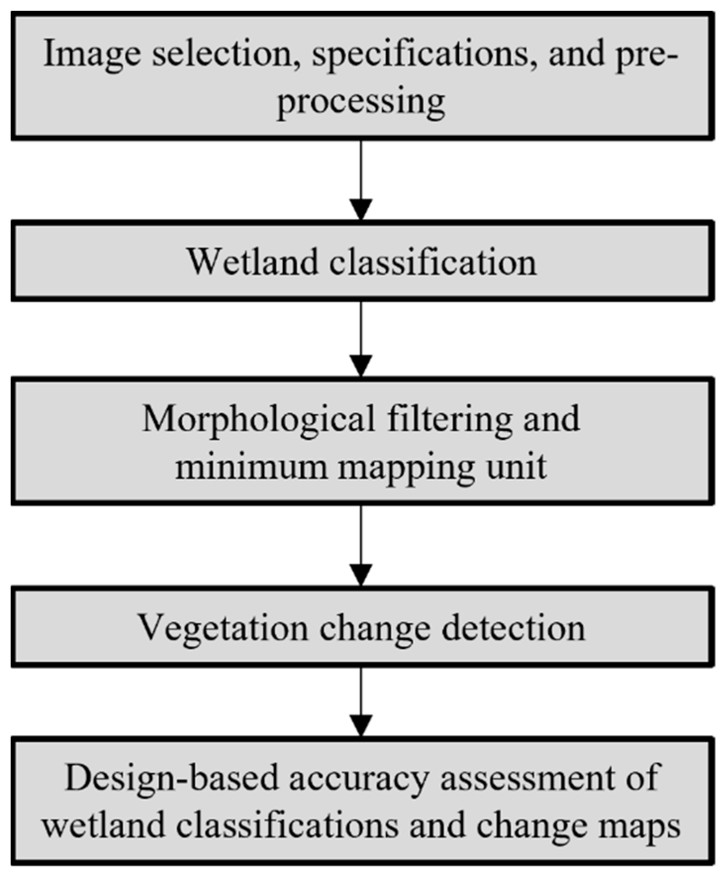
2. Methods
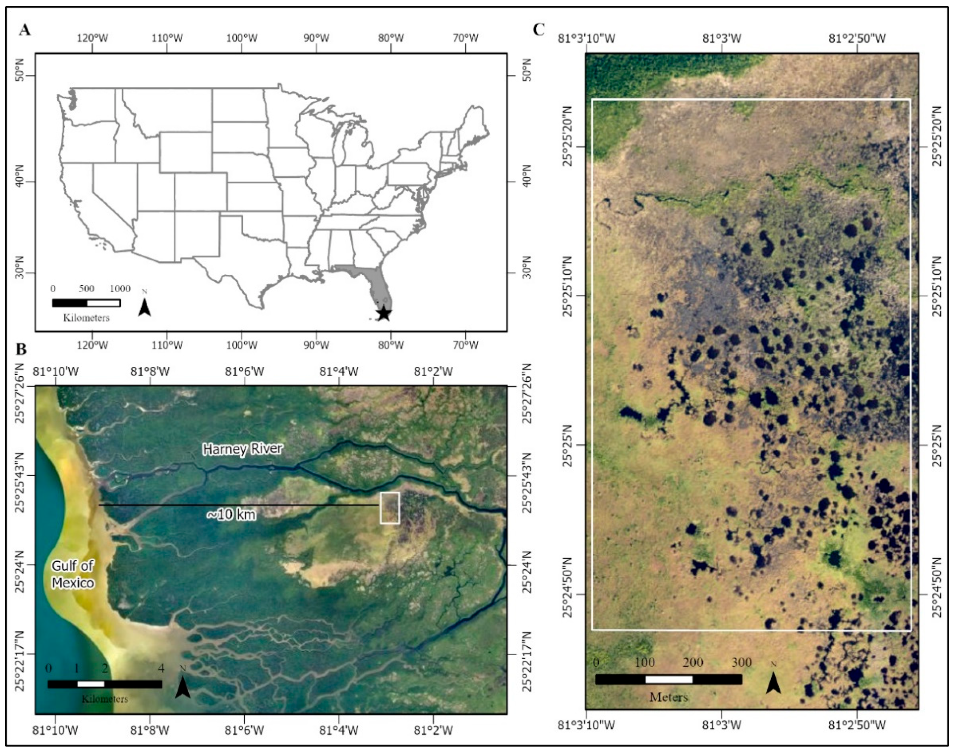
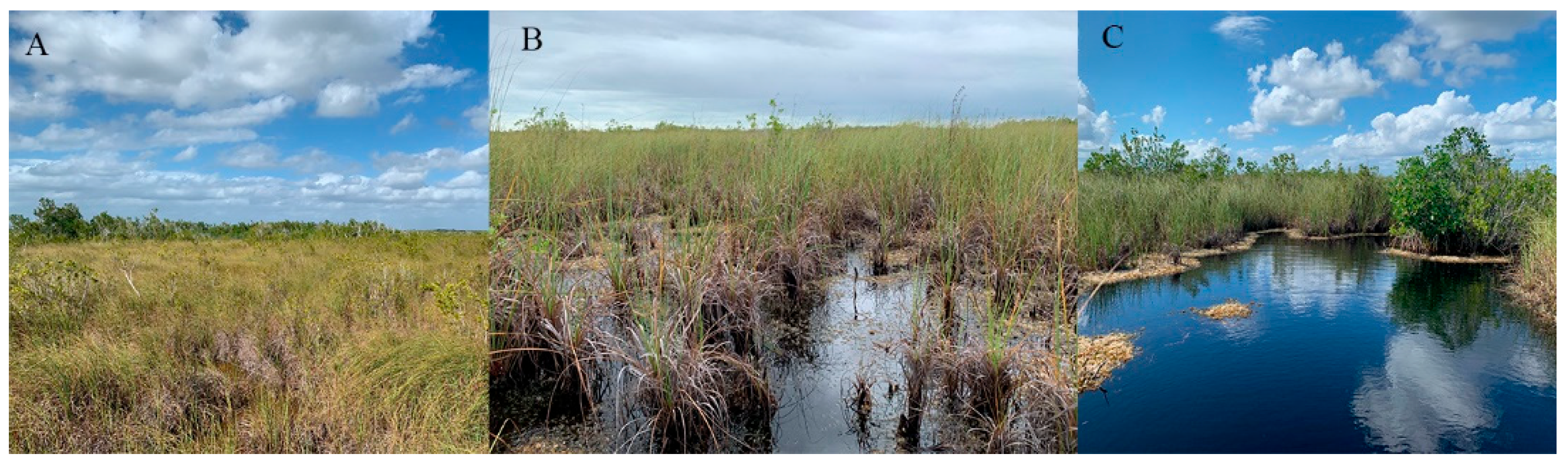
2.1. Study Area
2.2. Image Selection, Specifications, and Preprocessing
2.3. Wetland Classification
2.3.1. Classification Scheme
2.3.2. 1940 Manual Threshold Classification
2.3.3. 1940 and 2012 Automated Machine Learning Classification
2.4. Morphological Filtering and Minimum Mapping Unit
2.5. Vegetation Change Detection
2.6. Design-Based Accuracy Assessments of 1940 and 2012 Wetland Classifications and Change Maps
3. Results
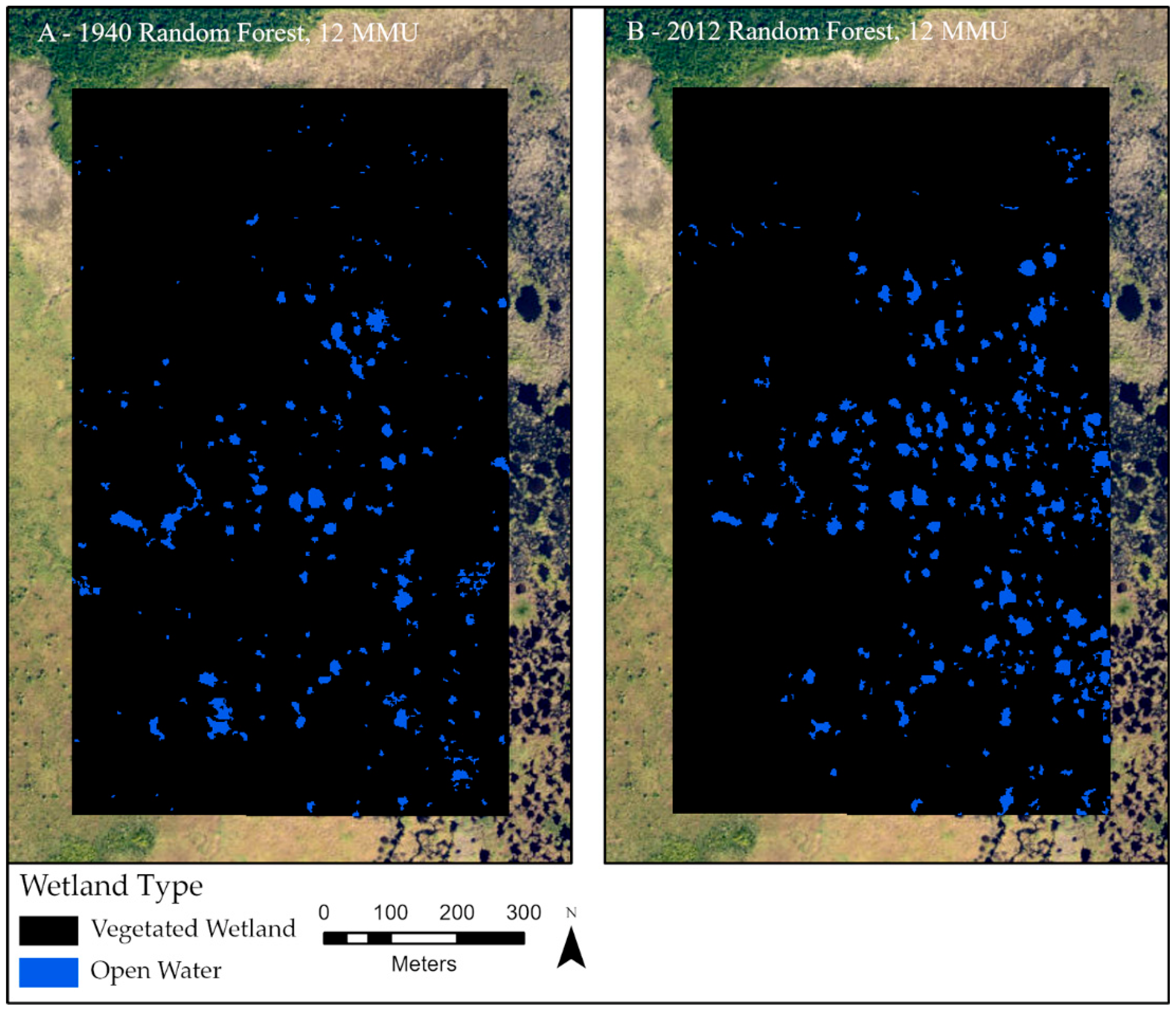
3.1. 1940 Wetland Classification
3.2. 2012 Wetland Classification
3.3. Changes in Wetland Classes from 1940 to 2012
3.4. Open Water Pond Detections: Total Count and Size
4. Discussion
4.1. The Importance of Spatially Explicit Accuracy Assessments
4.2. Misclassifications and Improving Accuracy
4.3. Impact of the Minimum Mapping Unit on Open Water Detection
4.4. Ecological Implications
5. Conclusions
Supplementary Materials
Author Contributions
Funding
Data Availability Statement
Acknowledgments
Conflicts of Interest
References
- Barbier, E.B.; Hacker, S.D.; Kennedy, C.; Koch, E.W.; Stier, A.C.; Silliman, B.R. The value of estuarine and coastal ecosystem services. Ecol. Monogr. 2011, 81, 169–193. [Google Scholar] [CrossRef]
- Mitsch, W.J.; Gosselink, J.G. Wetlands; John Wiley & Sons: New York, NY, USA, 2015; p. 752. [Google Scholar]
- Davidson, N.C.; Fluet-Chouinard, E.; Finlayson, C.M. Global extent and distribution of wetlands: Trends and issues. Mar. Freshw. Res. 2018, 69, 620–627. [Google Scholar] [CrossRef]
- Davidson, N.; Van Dam, A.; Finlayson, C.; McInnes, R. Worth of wetlands: Revised global monetary values of coastal and inland wetland ecosystem services. Mar. Freshw. Res. 2019, 70, 1189–1194. [Google Scholar] [CrossRef]
- Mcleod, E.; Chmura, G.L.; Bouillon, S.; Salm, R.; Björk, M.; Duarte, C.M.; Lovelock, C.E.; Schlesinger, W.H.; Silliman, B.R. A blueprint for blue carbon: Toward an improved understanding of the role of vegetated coastal habitats in sequestering CO2. Front. Ecol. Environ. 2011, 9, 552–560. [Google Scholar] [CrossRef]
- Kirwan, M.L.; Megonigal, J.P. Tidal wetland stability in the face of human impacts and sea-level rise. Nature 2013, 504, 53–60. [Google Scholar] [CrossRef] [PubMed]
- Osland, M.J.; Enwright, N.M.; Day, R.H.; Gabler, C.A.; Stagg, C.L.; Grace, J.B. Beyond just sea-level rise: Considering macroclimatic drivers within coastal wetland vulnerability assessments to climate change. Glob. Change Biol. 2016, 22, 1–11. [Google Scholar] [CrossRef]
- Osland, M.J.; Gabler, C.A.; Grace, J.B.; Day, R.H.; McCoy, M.L.; McLeod, J.L.; From, A.S.; Enwright, N.M.; Feher, L.C.; Stagg, C.L. Climate and plant controls on soil organic matter in coastal wetlands. Glob. Change Biol. 2018, 24, 5361–5379. [Google Scholar] [CrossRef]
- Osland, M.J.; Grace, J.B.; Guntenspergen, G.R.; Thorne, K.M.; Carr, J.A.; Feher, L.C. Climatic controls on the distribution of foundation plant species in coastal wetlands of the conterminous United States: Knowledge gaps and emerging research needs. Estuaries Coasts 2019, 42, 1991–2003. [Google Scholar] [CrossRef]
- Herbert, E.R.; Boon, P.; Burgin, A.J.; Neubauer, S.C.; Franklin, R.B.; Ardón, M.; Hopfensperger, K.N.; Lamers, L.P.; Gell, P. A global perspective on wetland salinization: Ecological consequences of a growing threat to freshwater wetlands. Ecosphere 2015, 6, 1–43. [Google Scholar] [CrossRef]
- Cahoon, D.R.; McKee, K.L.; Morris, J.T. How Plants Influence Resilience of Salt Marsh and Mangrove Wetlands to Sea-Level Rise. Estuaries Coasts 2020, 44, 883–898. [Google Scholar] [CrossRef]
- Cahoon, D.R.; Hensel, P.F.; Spencer, T.; Reed, D.J.; McKee, K.L.; Saintilan, N. Coastal wetland vulnerability to relative sea-level rise: Wetland elevation trends and process controls. In Wetlands and Natural Resource Management; Springer: Berlin/Heidelberg, Germany, 2006; pp. 271–292. [Google Scholar]
- Day, J.W.; Christian, R.R.; Boesch, D.M.; Yáñez-Arancibia, A.; Morris, J.; Twilley, R.R.; Naylor, L.; Schaffner, L. Consequences of climate change on the ecogeomorphology of coastal wetlands. Estuaries Coasts 2008, 31, 477–491. [Google Scholar] [CrossRef]
- Morris, J.T.; Sundareshwar, P.; Nietch, C.T.; Kjerfve, B.; Cahoon, D.R. Responses of coastal wetlands to rising sea level. Ecology 2002, 83, 2869–2877. [Google Scholar] [CrossRef]
- Schepers, L.; Kirwan, M.; Guntenspergen, G.; Temmerman, S. Spatio-temporal development of vegetation die-off in a submerging coastal marsh. Limnol. Oceanogr. 2017, 62, 137–150. [Google Scholar] [CrossRef]
- Andres, K.; Savarese, M.; Bovard, B.; Parsons, M. Coastal wetland geomorphic and vegetative change: Effects of Sea-level rise and water management on brackish marshes. Estuaries Coasts 2019, 42, 1308–1327. [Google Scholar] [CrossRef]
- Chambers, L.G.; Steinmuller, H.E.; Breithaupt, J.L. Toward a mechanistic understanding of “peat collapse” and its potential contribution to coastal wetland loss. Ecology 2019, 100, e02720. [Google Scholar] [CrossRef]
- Wilson, B.J.; Servais, S.; Charles, S.P.; Davis, S.E.; Gaiser, E.E.; Kominoski, J.S.; Richards, J.H.; Troxler, T.G. Declines in plant productivity drive carbon loss from brackish coastal wetland mesocosms exposed to saltwater intrusion. Estuaries Coasts 2018, 41, 2147–2158. [Google Scholar] [CrossRef]
- Charles, S.P.; Kominoski, J.S.; Troxler, T.G.; Gaiser, E.E.; Servais, S.; Wilson, B.J.; Davis, S.E.; Sklar, F.H.; Coronado-Molina, C.; Madden, C.J. Experimental Saltwater Intrusion Drives Rapid Soil Elevation and Carbon Loss in Freshwater and Brackish Everglades Marshes. Estuaries Coasts 2019, 42, 1868–1881. [Google Scholar] [CrossRef]
- National Academies of Sciences, Engineering, and Medicine. Progress Toward Restoring the Everglades: The Seventh Biennial Review—2018; National Academies Press: Cambridge, MA, USA, 2019. [Google Scholar]
- Hardisky, M.; Gross, M.; Klemas, V. Remote sensing of coastal wetlands. Bioscience 1986, 36, 453–460. [Google Scholar] [CrossRef]
- Ozesmi, S.L.; Bauer, M.E. Satellite remote sensing of wetlands. Wetl. Ecol. Manag. 2002, 10, 381–402. [Google Scholar] [CrossRef]
- Klemas, V. Remote sensing techniques for studying coastal ecosystems: An overview. J. Coast. Res. 2011, 27, 2–17. [Google Scholar]
- Rundquist, D.C.; Narumalani, S.; Narayanan, R.M. A review of wetlands remote sensing and defining new considerations. Remote Sens. Rev. 2001, 20, 207–226. [Google Scholar] [CrossRef]
- Adam, E.; Mutanga, O.; Rugege, D. Multispectral and hyperspectral remote sensing for identification and mapping of wetland vegetation: A review. Wetl. Ecol. Manag. 2010, 18, 281–296. [Google Scholar] [CrossRef]
- Moffett, K.B.; Nardin, W.; Silvestri, S.; Wang, C.; Temmerman, S. Multiple stable states and catastrophic shifts in coastal wetlands: Progress, challenges, and opportunities in validating theory using remote sensing and other methods. Remote Sens. 2015, 7, 10184–10226. [Google Scholar] [CrossRef]
- Guo, M.; Li, J.; Sheng, C.; Xu, J.; Wu, L. A review of wetland remote sensing. Sensors 2017, 17, 777. [Google Scholar] [CrossRef] [PubMed]
- Mahdavi, S.; Salehi, B.; Granger, J.; Amani, M.; Brisco, B.; Huang, W. Remote sensing for wetland classification: A comprehensive review. GIScience Remote Sens. 2018, 55, 623–658. [Google Scholar] [CrossRef]
- Belgiu, M.; Drăguţ, L. Random forest in remote sensing: A review of applications and future directions. ISPRS J. Photogramm. Remote Sens. 2016, 114, 24–31. [Google Scholar] [CrossRef]
- Breiman, L. Random forests. Mach. Learn. 2001, 45, 5–32. [Google Scholar] [CrossRef]
- Whiteside, T.G.; Bartolo, R.E. Mapping aquatic vegetation in a tropical wetland using high spatial resolution multispectral satellite imagery. Remote Sens. 2015, 7, 11664–11694. [Google Scholar] [CrossRef]
- Franklin, S.E.; Ahmed, O.S. Object-based wetland characterization using radarsat-2 quad-polarimetric SAR data, landsat-8 OLI imagery, and airborne lidar-derived geomorphometric variables. Photogramm. Eng. Remote Sens. 2017, 83, 27–36. [Google Scholar] [CrossRef]
- Mutanga, O.; Adam, E.; Cho, M.A. High density biomass estimation for wetland vegetation using WorldView-2 imagery and random forest regression algorithm. Int. J. Appl. Earth Obs. Geoinf. 2012, 18, 399–406. [Google Scholar] [CrossRef]
- Wendelberger, K.S.; Gann, D.; Richards, J.H. Using Bi-seasonal worldview-2 multi-spectral data and supervised random forest classification to map coastal plant communities in Everglades National Park. Sensors 2018, 18, 829. [Google Scholar] [CrossRef] [PubMed]
- Morgan, J.L.; Gergel, S.E.; Coops, N.C. Aerial photography: A rapidly evolving tool for ecological management. BioScience 2010, 60, 47–59. [Google Scholar] [CrossRef]
- Work, E.A.; Gilmer, D.S. Utilization of satellite data for inventorying prairie ponds and lakes. Photogramm. Eng. Remote Sens. 1976, 42, 685–694. [Google Scholar]
- Lyon, J.G.; Greene, R. Use of aerial photographs to measure the historical areal extent of Lake Erie coastal wetlands. Photogramm. Eng. Remote Sens. 1992, 58, 1355–1360. [Google Scholar]
- Williams, D.C.; Lyon, J.G. Historical aerial photographs and a geographic information system (GIS) to determine effects of long-term water level fluctuations on wetlands along the St. Marys River, Michigan, USA. Aquat. Bot. 1997, 58, 363–378. [Google Scholar] [CrossRef]
- Cserhalmi, D.; Nagy, J.; Kristóf, D.; Neidert, D. Changes in a wetland ecosystem: A vegetation reconstruction study based on historical panchromatic aerial photographs and succession patterns. Folia Geobot. 2011, 46, 351–371. [Google Scholar] [CrossRef]
- Ballanti, L.; Byrd, K.B.; Woo, I.; Ellings, C. Remote sensing for wetland mapping and historical change detection at the Nisqually River Delta. Sustainability 2017, 9, 1919. [Google Scholar] [CrossRef]
- Rapinel, S.; Clément, B.; Dufour, S.; Hubert-Moy, L. Fine-scale monitoring of long-term wetland loss using LiDAR data and historical aerial photographs: The example of the couesnon floodplain, France. Wetlands 2018, 38, 423–435. [Google Scholar] [CrossRef]
- Lillesand, T.M.; Kiefer, R.W.; Chipman, J. Remote Sensing and Image Interpretation; John Willey & Sons. Inc.: Hoboken, NJ, USA, 1994. [Google Scholar]
- Saura, S. Effects of minimum mapping unit on land cover data spatial configuration and composition. Int. J. Remote Sens. 2002, 23, 4853–4880. [Google Scholar] [CrossRef]
- Knight, J.F.; Lunetta, R.S. An experimental assessment of minimum mapping unit size. IEEE Trans. Geosci. Remote Sens. 2003, 41, 2132–2134. [Google Scholar] [CrossRef]
- Rutchey, K.; Godin, J. Determining an appropriate minimum mapping unit in vegetation mapping for ecosystem restoration: A case study from the Everglades, USA. Landsc. Ecol. 2009, 24, 1351–1362. [Google Scholar] [CrossRef]
- Lodge, T.E. The Everglades Handbook: Understanding the Ecosystem; CRC Press: Boca Raton, FL, USA, 2016. [Google Scholar]
- Yao, Q.; Liu, K.-B. Dynamics of marsh-mangrove ecotone since the mid-Holocene: A palynological study of mangrove encroachment and sea level rise in the Shark River Estuary, Florida. PLoS ONE 2017, 12, e0173670. [Google Scholar] [CrossRef] [PubMed]
- Scholl, D.W. Recent sedimentary record in mangrove swamps and rise in sea level over the southwestern coast of Florida: Part 2. Mar. Geol. 1964, 2, 343–364. [Google Scholar] [CrossRef]
- Smith, W.G. Sedimentary Environments and Environmental Change in the Peat-Forming Area of South Florida. Ph.D. Thesis, The Pennsylvania State University, State College, PA, USA, 1970. [Google Scholar]
- Parkinson, R.W. Decelerating Holocene sea-level rise and its influence on Southwest Florida coastal evolution; a transgressive/regressive stratigraphy. J. Sediment. Res. 1989, 59, 960–972. [Google Scholar]
- Kaplan, S.W. Peat Records of Late Holocene Climate and Sea Level Change in South Florida. Ph.D. Thesis, University of Wisconsin–Madison, Madison, WI, USA, 2004. [Google Scholar]
- Volety, A.K.; Savarese, M.; Hoye, B.; Loh, A.N. Landscape Pattern: Present and Past Distribution of Oysters in South Florida Coastal Complex (Whitewater Bay/Oyster Bay/Shark to Robert’s Rivers); South Florida Water Management District Final Technical Report; Florida Gulf Coast University: West Palm Beach, FL, USA, 2009. [Google Scholar]
- Davis, S.; Ogden, J.C. Everglades: The Ecosystem and Its Restoration; CRC Press: Boca Raton, FL, USA, 1994. [Google Scholar]
- Childers, D.L.; Gaiser, E.; Ogden, L.A. The Coastal Everglades: The Dynamics of Social-Ecological Transformation in the South Florida Landscape; Oxford University Press: Oxford, UK, 2019. [Google Scholar]
- McVoy, C.; Said, W.P.; Obeysekera, J.; VanArman, J.A.; Dreschel, T.W. Landscapes and Hydrology of the Predrainage Everglades; University Press of Florida Gainesville: Gainesville, FL, USA, 2011. [Google Scholar]
- Aich, S.; McVoy, C.W.; Dreschel, T.W.; Santamaria, F. Estimating soil subsidence and carbon loss in the Everglades Agricultural Area, Florida using geospatial techniques. Agric. Ecosyst. Environ. 2013, 171, 124–133. [Google Scholar] [CrossRef]
- Hohner, S.M.; Dreschel, T.W. Everglades peats: Using historical and recent data to estimate predrainage and current volumes, masses and carbon contents. Mires Peat. 2015, 16, 1–15. [Google Scholar]
- Foster, A. Historic Aerial Photography of the Greater Everglades Archive and Geodatabase Development; USGS Publications Warehouse: Restond, VA, USA, 2004; pp. 2327–6932.
- Hijmans, R.J.; Van Etten, J.; Cheng, J.; Mattiuzzi, M.; Sumner, M.; Greenberg, J.A.; Lamigueiro, O.P.; Bevan, A.; Racine, E.B.; Shortridge, A. Raster: Geographic Data Analysis and Modeling. R Package Version 2.8-4. 2015. Available online: https://CRAN.R-project.org/package=raster (accessed on 19 June 2022).
- Kuhn, M.; Wing, J.; Weston, S.; Williams, A.; Keefer, C.; Engelhardt, A.; Cooper, T.; Mayer, Z.; Kenkel, B.; Team, R.C. Caret: Classification and Regression Training. R Package Version 6.0-80. 2020. Available online: https://CRAN.R-project.org/package=caret (accessed on 19 June 2022).
- Jordan, C.F. Derivation of leaf-area index from quality of light on the forest floor. Ecology 1969, 50, 663–666. [Google Scholar] [CrossRef]
- Rousel, J.; Haas, R.; Schell, J.; Deering, D. Monitoring Vegetation Systems in the Great Plains with ERTS. In Proceedings of the Third Earth Resources Technology Satellite—1 Symposium, NASA SP-351, Washington, DC, USA, 10–14 December 1973; pp. 309–317. [Google Scholar]
- Barnes, E.; Clarke, T.; Richards, S.; Colaizzi, P.; Haberland, J.; Kostrzewski, M.; Waller, P.; Choi, C.; Riley, E.; Thompson, T. Coincident detection of crop water stress, nitrogen status and canopy density using ground based multispectral data. In Proceedings of the Fifth International Conference on Precision Agriculture, Bloomington, MN, USA, 16–19 July 2000; p. 6. [Google Scholar]
- McFeeters, S.K. The use of the Normalized Difference Water Index (NDWI) in the delineation of open water features. Int. J. Remote Sens. 1996, 17, 1425–1432. [Google Scholar] [CrossRef]
- Gitelson, A.A.; Kaufman, Y.J.; Merzlyak, M.N. Use of a green channel in remote sensing of global vegetation from EOS-MODIS. Remote Sens. Environ. 1996, 58, 289–298. [Google Scholar] [CrossRef]
- Huete, A.R. A soil-adjusted vegetation index (SAVI). Remote Sens. Environ. 1988, 25, 295–309. [Google Scholar] [CrossRef]
- Jiang, Z.; Huete, A.R.; Didan, K.; Miura, T. Development of a two-band enhanced vegetation index without a blue band. Remote Sens. Environ. 2008, 112, 3833–3845. [Google Scholar] [CrossRef]
- Serra, J. Introduction to mathematical morphology. Comput. Vis. Graph. Image Processing 1986, 35, 283–305. [Google Scholar] [CrossRef]
- Heijmans, H.J. Mathematical morphology: A modern approach in image processing based on algebra and geometry. SIAM Rev. 1995, 37, 1–36. [Google Scholar] [CrossRef]
- Soille, P.; Pesaresi, M. Advances in mathematical morphology applied to geoscience and remote sensing. IEEE Trans. Geosci. Remote Sens. 2002, 40, 2042–2055. [Google Scholar] [CrossRef]
- R Core Team. R: A Language and Environment for Statistical Computing; R Foundation for Statistical Computing: Vienna, Austria, 2022. [Google Scholar]
- Jensen, J.R. Introductory Digital Image Processing: A Remote Sensing Perspective; Prentice-Hall Inc.: Hoboken, NJ, USA, 1996. [Google Scholar]
- Tillé, Y.; Matei, A.; Sampling: Survey Sampling. R Package Version 2.8. 2012. Available online: https://CRAN.R-project.org/package=sampling (accessed on 19 June 2022).
- Olofsson, P.; Foody, G.M.; Herold, M.; Stehman, S.V.; Woodcock, C.E.; Wulder, M.A. Good practices for estimating area and assessing accuracy of land change. Remote Sens. Environ. 2014, 148, 42–57. [Google Scholar] [CrossRef]
- McCarthy, M.J.; Jessen, B.; Barry, M.J.; Figueroa, M.; McIntosh, J.; Murray, T.; Schmid, J.; Muller-Karger, F.E. Automated high-resolution time series mapping of mangrove forests damaged by hurricane Irma in Southwest Florida. Remote Sens. 2020, 12, 1740. [Google Scholar] [CrossRef]
- Wood, E.M.; Pidgeon, A.M.; Radeloff, V.C.; Keuler, N.S. Image texture as a remotely sensed measure of vegetation structure. Remote Sens. Environ. 2012, 121, 516–526. [Google Scholar] [CrossRef]
- Hudak, A.T.; Wessman, C.A. Textural analysis of historical aerial photography to characterize woody plant encroachment in South African savanna. Remote Sens. Environ. 1998, 66, 317–330. [Google Scholar] [CrossRef]
- Caridade, C.; Marçal, A.R.; Mendonça, T. The use of texture for image classification of black & white air photographs. Int. J. Remote Sens. 2008, 29, 593–607. [Google Scholar]
- Biskup, B.; Scharr, H.; Schurr, U.; Rascher, U. A stereo imaging system for measuring structural parameters of plant canopies. Plant Cell Environ. 2007, 30, 1299–1308. [Google Scholar] [CrossRef]
- U.S. Army Corps of Engineers. Comprehensive Everglades Restoration Plan: Picayune Strand Restoration (Formally the South Golden Gate Estates Ecosystem Restoration); United States Army Corps of Engineers: Washington, DC, USA, 2004; p. 488.
- Sklar, F.H.; Meeder, J.F.; Troxler, T.G.; Dreschel, T.; Davis, S.E.; Ruiz, P.L. The Everglades: At the Forefront of Transition. In Coasts and Estuaries; Elsevier: Amsterdam, The Netherlands, 2019; pp. 277–292. [Google Scholar]
- DeLaune, R.D.; Nyman, J.A.; Patrick Jr, W. Peat collapse, ponding and wetland loss in a rapidly submerging coastal marsh. J. Coast. Res. 1994, 4, 1021–1030. [Google Scholar]
- Wilson, B.J.; Servais, S.; Mazzei, V.; Kominoski, J.S.; Hu, M.; Davis, S.E.; Gaiser, E.; Sklar, F.; Bauman, L.; Kelly, S. Salinity pulses interact with seasonal dry-down to increase ecosystem carbon loss in marshes of the Florida Everglades. Ecol. Appl. 2018, 28, 2092–2108. [Google Scholar] [CrossRef] [PubMed]
- Solohin, E.; Widney, S.E.; Craft, C.B. Declines in plant productivity drive loss of soil elevation in a tidal freshwater marsh exposed to saltwater intrusion. Ecology 2020, 101, e03148. [Google Scholar] [CrossRef] [PubMed]
- Cahoon, D.R.; Hensel, P.; Rybczyk, J.; McKee, K.L.; Proffitt, C.E.; Perez, B.C. Mass tree mortality leads to mangrove peat collapse at Bay Islands, Honduras after Hurricane Mitch. J. Ecol. 2003, 91, 1093–1105. [Google Scholar] [CrossRef]
- Day, J.W.; Kemp, G.P.; Reed, D.J.; Cahoon, D.R.; Boumans, R.M.; Suhayda, J.M.; Gambrell, R. Vegetation death and rapid loss of surface elevation in two contrasting Mississippi delta salt marshes: The role of sedimentation, autocompaction and sea-level rise. Ecol. Eng. 2011, 37, 229–240. [Google Scholar] [CrossRef]
- Schepers, L.; Brennand, P.; Kirwan, M.L.; Guntenspergen, G.R.; Temmerman, S. Coastal Marsh Degradation Into Ponds Induces Irreversible Elevation Loss Relative to Sea Level in a Microtidal System. Geophys. Res. Lett. 2020, 47, e2020GL089121. [Google Scholar] [CrossRef]
- Wang, C.; Schepers, L.; Kirwan, M.L.; Belluco, E.; D’Alpaos, A.; Wang, Q.; Yin, S.; Temmerman, S. Different coastal marsh sites reflect similar topographic conditions under which bare patches and vegetation recovery occur. Earth Surf. Dyn. 2021, 9, 71–88. [Google Scholar] [CrossRef]
- Parkinson, R.W.; Wdowinski, S. Accelerating sea-level rise and the fate of mangrove plant communities in South Florida, USA. Geomorphology 2022, 412, e108329. [Google Scholar] [CrossRef]
- Schuerch, M.; Spencer, T.; Temmerman, S.; Kirwan, M.L.; Wolff, C.; Lincke, D.; McOwen, C.J.; Pickering, M.D.; Reef, R.; Vafeidis, A.T. Future response of global coastal wetlands to sea-level rise. Nature 2018, 561, 231–234. [Google Scholar] [CrossRef]


| Band/Vegetation Index | Equation | Reference |
|---|---|---|
| Red, Blue, Green, Coastal, Red, NIR1, NRI2, RE | None | N/A |
| Simple Ratio (SR) | Red/NIR1 | [61] |
| Normalized Difference Vegetation Index (NDVI) | (NIR1 − Red)/ (NIR1 + Red) | [62] |
| Normalized Difference Red-Edge Index (NDRE) | (NIR1 − RE)/ (NIR1 + RE) | [63] |
| Normalized Difference Water Index (NDWI) | (Green-NIR2)/(Green + NIR2) | [64] |
| Green Normalized Difference Vegetation Index (GNDVI) | (NIR1-Green)/(NIR1 + Green) | [65] |
| Soil Adjusted Vegetation Index (SAVI) | 1.5 × ((NIR1 − Red)/ (NIR1 + Red + 0.5)) | [66] |
| Enhanced Vegetation Index (EVI) | 2.5 × ((NIR1 − Red)/ (NIR1 + 2.4 × Red + 1)) | [67] |
| Year and Method | MMU (m2) | Class | Mapped Area (ha) | Adjusted Area (ha) | Adjusted Producer’s Accuracy | Adjusted User’s Accuracy | Overall Accuracy |
|---|---|---|---|---|---|---|---|
| 1940 Thres | 12 | Vegetated | 70.4 | 70.6 ± 0.1 | 99.8 ± 0.1 | 100 ± 0.0 | 99.8 ± 0.1 |
| Open water | 1.5 | 1.4 ± 0.1 | 100 ± 0.0 | 91.5 ± 7.2 | |||
| 24 | Vegetated | 70.5 | 69.4 ± 2.5 | 99.7 ± 0.2 | 96.4 ± 4.9 | 96.2 ± 4.8 | |
| Open water | 1.5 | 2.6 ± 2.5 | 50.1 ± 49.2 | 87.5 ± 8.7 | |||
| 36 | Vegetated | 70.6 | 70.7 ± 0.1 | 99.8 ± 0.2 | 100 ± 0.0 | 98.8 ± 0.1 | |
| Open water | 1.4 | 1.3 ± 0.1 | 100 ± 0.0 | 90.6 ± 0.4 | |||
| 1940 rF | 12 | Vegetated | 69.8 | 70.2 ± 0.1 | 99.7 ± 0.2 | 100 ± 0.0 | 99.7 ± 0.1 |
| Open water | 2.2 | 1.8 ± 0.1 | 100 ± 0.0 | 90.4 ± 6.8 | |||
| 24 | Vegetated | 69.9 | 70.2 ± 0.2 | 99.5 ± 0.2 | 100 ± 0.0 | 99.5 ± 0.2 | |
| Open water | 2.0 | 1.7 ± 0.2 | 100 ± 0.0 | 83.1 ± 8.4 | |||
| 36 | Vegetated | 70.0 | 70.2 ± 0.1 | 99.7 ± 0.2 | 100 ± 0.0 | 99.5 ± 0.2 | |
| Open water | 1.9 | 1.8 ± 0.1 | 100 ± 0.0 | 90.4 ± 6.8 | |||
| 2012 rF | 12 | Vegetated | 68.5 | 68.1 ± 1.1 | 99.8 ± 0.1 | 99.2 ± 1.5 | 99.1 ± 1.5 |
| Open water | 3.5 | 3.9 ± 1.1 | 86.3 ± 23.2 | 96.8 ± 3.0 | |||
| 24 | Vegetated | 68.6 | 67.1 ± 1.8 | 99.8 ± 0.1 | 97.6 ± 2.7 | 97.6 ± 2.6 | |
| Open water | 3.4 | 4.9 ± 1.8 | 66.5 ± 25.0 | 96.8 ± 3.1 | |||
| 36 | Vegetated | 68.7 | 68.1 ± 1.1 | 99.9 ± 0.1 | 99.1 ± 1.6 | 99.2 ± 1.5 | |
| Open water | 3.3 | 3.8 ± 1.1 | 85.1 ± 12.6 | 99.9 ± 1.6 |
| Change Map | MMU (m2) | Class | Mapped Area (ha) | Adjusted Area (ha) | Adjusted Producer’s Accuracy | Adjusted User’s Accuracy | Overall Accuracy |
|---|---|---|---|---|---|---|---|
| 1940 Thres, 2012 rF | 12 | No Change | 68.6 | 69.3 ± 0.2 | 98.9 ± 0.3 | 100 ± 0.0 | 99.0 ± 0.3 |
| Vegetated to Water | 2.7 | 2.2 ± 0.2 | 100 ± 0.0 | 81.1 ± 7.9 | |||
| Water to Vegetated | 0.7 | 0.5 ± 0.1 | 100 ± 0.0 | 72.6 ± 9.0 | |||
| 24 | No Change | 68.7 | 69.5 ± 0.2 | 98.9 ± 0.3 | 100 ± 0.0 | 98.9 ± 0.3 | |
| Vegetated to Water | 2.6 | 2.0 ± 0.2 | 100 ± 0.0 | 80.2 ± 8.2 | |||
| Water to Vegetated | 0.7 | 0.4 ± 0.1 | 100 ± 0.0 | 63.7 ± 9.9 | |||
| 36 | No Change | 68.9 | 69.0 ± 1.6 | 98.6 ± 0.3 | 98.8 ± 2.2 | 97.6 ± 2.2 | |
| Vegetated to Water | 2.5 | 2.5 ± 1.6 | 68.7 ± 42.3 | 70.1 ± 9.7 | |||
| Water to Vegetated | 0.6 | 0.4 ± 0.1 | 100 ± 0.0 | 68.9 ± 9.8 | |||
| 1940 rF, 2012 rF | 12 | No Change | 68.3 | 67.9 ± 1.8 | 98.6 ± 0.3 | 98.1 ± 2.6 | 96.9 ± 2.5 |
| Vegetated to Water | 2.5 | 3.4 ± 1.8 | 61.1 ± 32.9 | 83.5 ± 7.2 | |||
| Water to Vegetated | 1.2 | 0.7 ± 0.1 | 100 ± 0.0 | 57.3 ± 9.6 | |||
| 24 | No Change | 68.5 | 68.7 ± 1.4 | 98.6 ± 0.3 | 98.9 ± 1.9 | 98.7 ± 0.3 | |
| Vegetated to Water | 2.4 | 2.0 ± 0.2 | 100 ± 0.0 | 81.6 ± 7.7 | |||
| Water to Vegetated | 1.1 | 1.3 ± 1.4 | 100 ± 0.0 | 56.1 ± 9.8 | |||
| 36 | No Change | 68.6 | 68.9 ± 1.4 | 98.6 ± 0.3 | 98.9 ± 2.1 | 97.6 ± 2.0 | |
| Vegetated to Water | 2.4 | 2.5 ± 1.4 | 71.2 ± 40.2 | 77.6 ± 8.4 | |||
| Water to Vegetated | 1.0 | 0.5 ± 0.9 | 100 ± 0.0 | 53.2 ± 10.1 |
| Year, Classification-MMU | Total Open Water Body Detections | Median Open Water Area (m2) |
|---|---|---|
| 1940, Thres-12 | 172 | 43.0 |
| 1940, Thres-24 | 132 | 58.0 |
| 1940, Thres-36 | 103 | 80.0 |
| 1940, rF-12 | 251 | 32.0 |
| 1940, rF-24 | 161 | 70.0 |
| 1940, rF-36 | 125 | 87.0 |
| 2012, rF-12 | 307 | 55.0 |
| 2012, rF-24 | 232 | 84.5 |
| 2012, rF-36 | 197 | 97.0 |
Publisher’s Note: MDPI stays neutral with regard to jurisdictional claims in published maps and institutional affiliations. |
© 2022 by the authors. Licensee MDPI, Basel, Switzerland. This article is an open access article distributed under the terms and conditions of the Creative Commons Attribution (CC BY) license (https://creativecommons.org/licenses/by/4.0/).
Share and Cite
Lamb, L.M.; Gann, D.; Velazquez, J.T.; Troxler, T.G. Detecting Vegetation to Open Water Transitions in a Subtropical Wetland Landscape from Historical Panchromatic Aerial Photography and Multispectral Satellite Imagery. Remote Sens. 2022, 14, 3976. https://doi.org/10.3390/rs14163976
Lamb LM, Gann D, Velazquez JT, Troxler TG. Detecting Vegetation to Open Water Transitions in a Subtropical Wetland Landscape from Historical Panchromatic Aerial Photography and Multispectral Satellite Imagery. Remote Sensing. 2022; 14(16):3976. https://doi.org/10.3390/rs14163976
Chicago/Turabian StyleLamb, Lukas M., Daniel Gann, Jesse T. Velazquez, and Tiffany G. Troxler. 2022. "Detecting Vegetation to Open Water Transitions in a Subtropical Wetland Landscape from Historical Panchromatic Aerial Photography and Multispectral Satellite Imagery" Remote Sensing 14, no. 16: 3976. https://doi.org/10.3390/rs14163976
APA StyleLamb, L. M., Gann, D., Velazquez, J. T., & Troxler, T. G. (2022). Detecting Vegetation to Open Water Transitions in a Subtropical Wetland Landscape from Historical Panchromatic Aerial Photography and Multispectral Satellite Imagery. Remote Sensing, 14(16), 3976. https://doi.org/10.3390/rs14163976