Bidirectional Flow Decision Tree for Reliable Remote Sensing Image Scene Classification

Abstract

Remote sensing image scene classification (RSISC), which aims to classify scene categories for remote sensing imagery, has broad applications in various fields. Recent deep learning (DL) successes have led to a new wave of RSISC applications; however, they lack explainability and trustworthiness. Here, we propose a bidirectional flow decision tree (BFDT) module to create a reliable RS scene classification framework. Our algorithm combines BFDT and Convolutional Neural Networks (CNNs) to make the decision process easily interpretable. First, we extract multilevel feature information from the pretrained CNN model, which provides the basis for constructing the subsequent hierarchical structure. Then the model uses the discriminative nature of scene features at different levels to gradually refine similar subsets and learn the interclass hierarchy. Meanwhile, the last fully connected layer embeds decision rules for the decision tree from the bottom up. Finally, the cascading softmax loss is used to train and learn the depth features based on the hierarchical structure formed by the tree structure that contains rich remote sensing information. We also discovered that superclass results can be obtained well for unseen classes due to its unique tree structure hierarchical property, which results in our model having a good generalization effect. The experimental results align with theoretical predictions using three popular datasets. Our proposed framework provides explainable results, leading to correctable and trustworthy approaches.

1. Introduction

Recent advances in satellite sensor and remote sensing (RS) imaging technology enable high-resolution RS images, providing detailed spatial information about our world. Under this circumstance, remote sensing image scene classification (RSISC) has drawn significant attention due to its wide range of applications, such as national defense security [1], natural hazard detection [2], urban planning [3], and environmental monitoring [4]. While the high resolution of remotely sensed images brings valuable data for subsequent vision tasks, the intricate image details and structures make characterization modeling more challenging.

Early approaches mainly focused on handcrafted features, such as scale-invariant feature transform (SIFT) [5] and Gabor [6], local binary patterns (LBPs) [7], and histograms of oriented gradients (HOG) [8]. Thus, extracting high-level features from RS images becomes quite challenging. Due to its excellent feature extraction capabilities, advanced deep learning (DL) methods have been successfully applied to RSISC [9,10]. This approach assumes that a filter describes a mixture of patterns with weak feature interpretability as a data-driven method. For example, the filter may be activated by both the building and the road of the residential area. It cannot represent the same object or part across different RS images. The global features and detailed geometric information in RS images gradually weaken in the layer-by-layer convolution and subsampling.

In most RSISC tasks, maximizing classification accuracy is usually used as the sole objective. However, many applications are also interested in finding a user-friendly explainable classifier. First, it helps identify the essential rules responsible for the RSISC task. In addition, it provides a more direct relationship of features to gain better insight for future developmental purposes. A key challenge to improving the model’s interpretability is that the high-resolution properties of RS images are complicated to predict because DL methods do not focus on distinguishing critical information from redundant features in images. Meanwhile, explainability is often discussed as a technical challenge in designing DL systems and decision procedures. In contrast, the end-to-end learning procedure of DL causes it to be a black-box model. The “black box” raises questions about reliability, significantly limiting the value of the data used. Nevertheless, RSISC tasks are related to many critical applications, and explanations are essential for users to understand, trust, and have confidence in the prediction results.

To date, the limitation of deep neural networks (DNNs) for RSISC has not been fully explored. A strength of DL approaches is that they can learn independently without specific previous knowledge. However, even a well-trained model cannot adapt to an uncertain environment; thus, producing reliable results will be challenging because such models are typically only adapted to a specific domain. RS images have a prominent spatial feature correlation compared with the training image data for the traditional scene classification tasks. As a result, RSISC suffers from many additional challenges, such as the dense distribution of geospatial objects. Moreover, explainability is often a technical challenge in designing DL-based systems and decision procedures. Developing more accurate and reliable RSISC systems will improve and extend their applications.

Here, we address these issues by directly incorporating reliability and uncertainty into the model and utilizing a decision tree as the low complexity and explainability classifier. Decision trees (DTs) are widely used classifiers successfully employed in many application domains. The popularity of DTs is mainly due to the simplicity of their learning schema. Furthermore, DTs are considered among the most interpretable classifiers [8]. Note that our task of improving the interpretability of an RSISC is essentially different from conventional visualization. The BFDT visualizes the decision procedure with a tree-like structure, whereas previous methods mainly explain model predictions by identifying which pixels most affected the prediction. We provide two main components using the DL framework and decision tree model techniques. First, we introduce the BFDT, a DT algorithm with dynamic granularity. We progressively integrate rich spatial details and high-level semantic information in a top-down manner to achieve interpretable paths continuously. The weights of the corresponding parent nodes are obtained from the bottom-up using the leaf node weight values. Second, we derive the cascading softmax loss to train and learn the depth features based on the hierarchical structure with rich contextual information. This paper’s main contributions can be summarized as follows:

• To preserve interpretability and achieve competitive accuracy, we integrate the decision tree model into the CNNs and train it with the cascaded softmax loss to sufficiently mine RS images’ scene structures and essential visual features. The proposed method can learn more interpretable features instead of explaining pretrained neural networks.
• We efficiently incorporate the high performance of the bottom-up mode and the strong interpretability of the top-down manner while constructing semantic and layer-based visual remote sensing image hierarchies. Thus, it can capture the hierarchical structure of images from remote sensing and make visual decisions based on them. In addition, to the best of our knowledge, this work provides the first bidirectional feature-flow decision tree, which provides a reliable RSISC.
• The proposed framework has a degree of attribute discrimination that fully utilizes the decision tree’s decision-making advantages. Moreover, it provides joint improvement of accuracy and interpretability.

2. Related Work

2.1. Conventional CNN Features-Based Methods

Due to its excellent feature extraction capabilities, CNNs have been widely utilized in RSISC in recent competitive methods. Cheng et al. [11] extracted features from a pretrained model and subsequently classified them using linear SVM. Compared to traditional manual techniques such as SIFT [5], Gabor [6], histogram of oriented gradients (HOG) [8], etc., pretrained CNN features can provide more precise information to help the model describe the semantic meaning. Although these methods all achieve good performance, they focus only on the feature map of the final layer and ignore the vast amount of information contained in the rich intermediate layers of CNN. The low-level features from the lower convolutional layers are filled with symbolic spatial structure information. In contrast, the mid-level features from the upper convolutional layers contain more abstract semantic information that is not affected by pose, position, illumination, etc. [12]. Hence, utilizing features from multiple CNN layers may provide richer semantic information. Zhu et al. [13] proposed a method to integrate the completely sparse topic model with CNN and use the multi-level semantics of HSR scenes for scene classification. Hydra [14] mainly builds a CNN that provides a good starting point for rough optimization and further optimization and then uses different methods to fine-tune the obtained weights many times.

N. He et al. [15] combined features extracted from multilayer networks, from low-level figurative features to high-level abstract attributes, to learn more discriminative features for RSISC. Similarly, Liu et al. [16] even integrated multiple CNNs to combine the network layers to perform better. Akashdeep Goel et al. [17] further explored the apparent similarity of scenes by proposing a hierarchical structure approach. Zhang X et al. [18] constructed graph structures from objects generated from VHR RS images and used graph theory to fully exploit the correlation between objects. Xu et al. [19] combined lie group learning machine learning with CNN and proposed Lie Group Regional Influence Network (LGRIN) to achieve advanced results. Huang et al. [20] proposed scalable subspace clustering methods for highly redundant dictionaries due to sparse subspace clustering and introduced adaptive spatial regularization to improve the robustness of the model.

2.2. The Deep Learning Interpretable Method

While deep learning has been making enormous strides in various disciplines, its black-box peculiarity remains an unsolved challenge. Multiple approaches have been proposed to reveal the model’s decision-making basis or working mechanism [21]. Wei et al. [22] validate the applicability of gradient-weighted class activation mapping (Grad-CAM) in remote sensing image classification tasks and propose a new strategy to correct the visual interpretation generated by Grad-CAM. Huang et al. [23] reconstructed a remote sensing image using the extracted features, improving classification performance and obtaining a better visual interpretation. Wei et al. [24] used median pools to capture the main trends of gradients and approximate the contribution of feature maps to specific classes. It provides a good compromise between the interpretability and visual interpretability of RSISC models. These methods use significance maps to explain remote sensing image classification. Zhao et al. [25] exploited Riemannian fluidic feature space’s strong feature representation capability (RMFS) to bridge the gap between CNN and a priori knowledge of remote sensing images, thus realizing a CNN model with reasonable feature interpretation. However, they all pay attention to the inputs and ignore the model’s decision process.

Our BFDT model is inspired by the idea of using information from different CNN layers to obtain sequential decision processes [26,27]. The advantage of tree-based methods is that they efficiently describe decision manifolds with approximate hyperplane borders, which can be explained by tracking decision nodes. Boualleg et al. [10] proposed an integrated learning-based deep forest (DF) model that fully uses the CNN’s capability to extract features and DF classification interpretability to mine high-quality information from remote sensing scene images. A random forest classifier for hyperspectral remote sensing image classification was proposed in [28,29], improving classification performance. However, the forest becomes intractable because of the decision paths that follow the set of trees, thus sacrificing the intrinsic interpretability of the decision tree intuition. Chiranjibi Shah et al. [30] apply tabular data learning networks (TabNet): sequential attention to select the appropriate salient features at each decision step, resulting in interpretability, efficient learning, and improved learning ability. Hehn et al. [31] proposed a greedy tree structure formwork for constructing unbalanced DNDFs with data-specific structures to improve interpretability. However, this scheme is only applicable to small datasets. Hinton et al. [32] visualized high-dimensional data by giving each datapoint a location in a two or three-dimensional map.

2.3. The Deep Learning Methods in RSISC

Many DL methods have achieved impressive progress in RSISC. With a large-scale remote sensing image dataset [33,34,35] that contains rich scene categories, they use deep CNN as a local feature extractor and combine it with feature coding approaches. For example, Binary Patterns encoded CNNs [36], attention-based CNNs [37,38,39,40], lightweight structure [41,42], and multi-scale classification [43]. When encountering an uncertain real-world environment, it is necessary to approximate uncertainty in real-world environments [44]. In addition, many approaches have been developed for scale variation [45,46,47,48,49]. For example, Shen et al. [45] developed a pluggable importance factor generator for highly different scales, and Liu et al. [46] proposed a network to learn sparse and effective feature representations. The challenge, therefore, is in the unlabeled RS images. Consequently, Li et al. [50] proposed a geographical knowledge-driven representation learning method for RS images. Addressing time-consumption, Gao et al. [51] use the Low-Rank Nonlocal Representation, and He et al. [52] propose the Skip-Connected Covariance Network. The RSISC methods based on CNNs can be categorized as (1) methods that involve training from scratch and (2) using a pretrained CNN36 as a feature extractor. Moreover, various fusion technologies have been addressed [53,54,55,56,57]. Ji et al. [53] localized multiscale regions of the RS scene images, and combined features learned from the localized regions. Furthermore, there are other new strategies to further improve further performance, such as multilevel attention modules [19], multi-granularity appearance pooling models [58], self-training algorithms [59], and joint decisions [60]. However, none of these methods achieved the subgenus specificity required for discriminating.

Compared to previous works, our approach visualizes the decision procedure with a tree-like structure while protecting the accuracy of the RSISC. Moreover, the decision tree in our work is close to the human reasoning process and more interpretable.

3. Methods

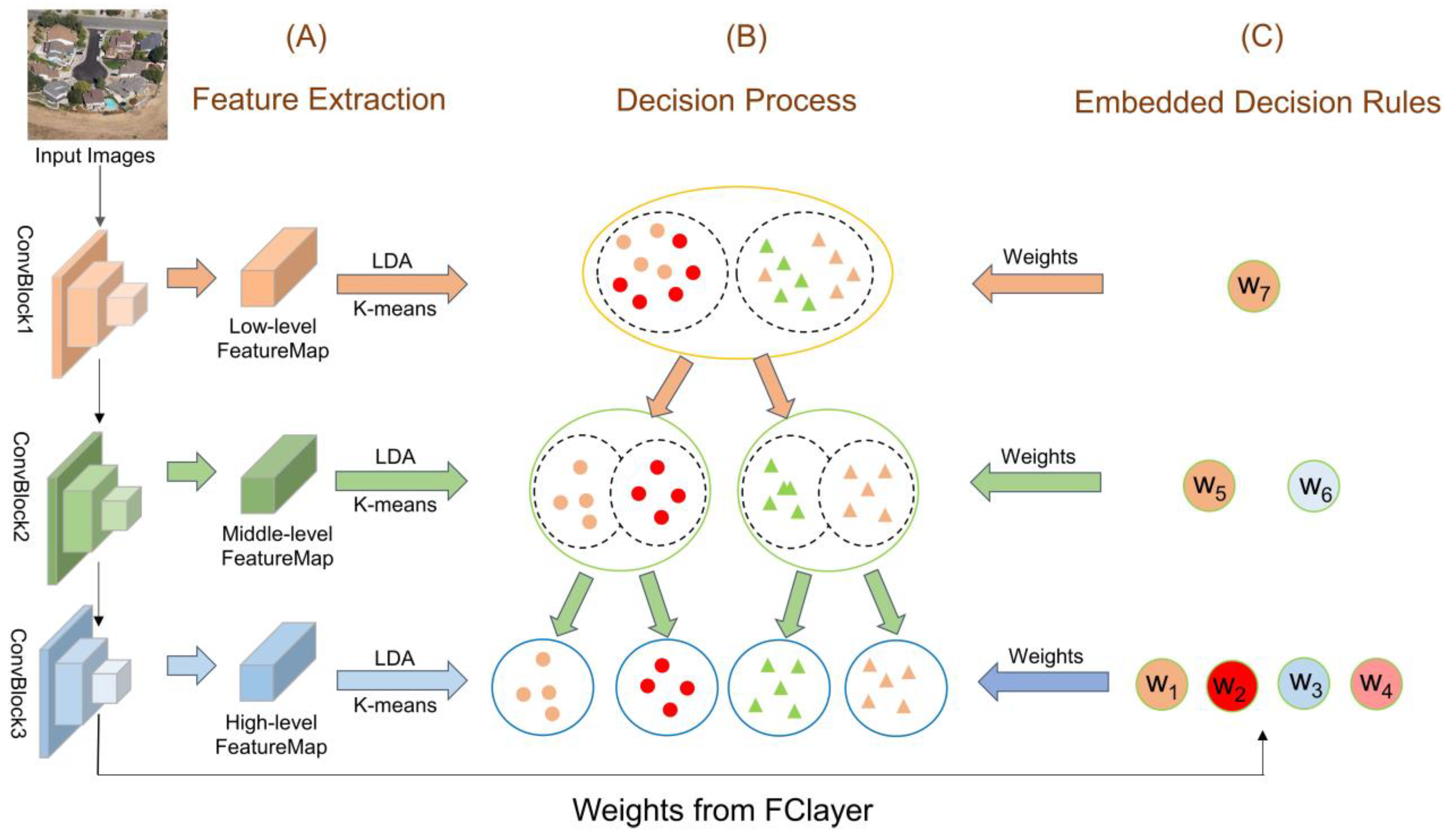
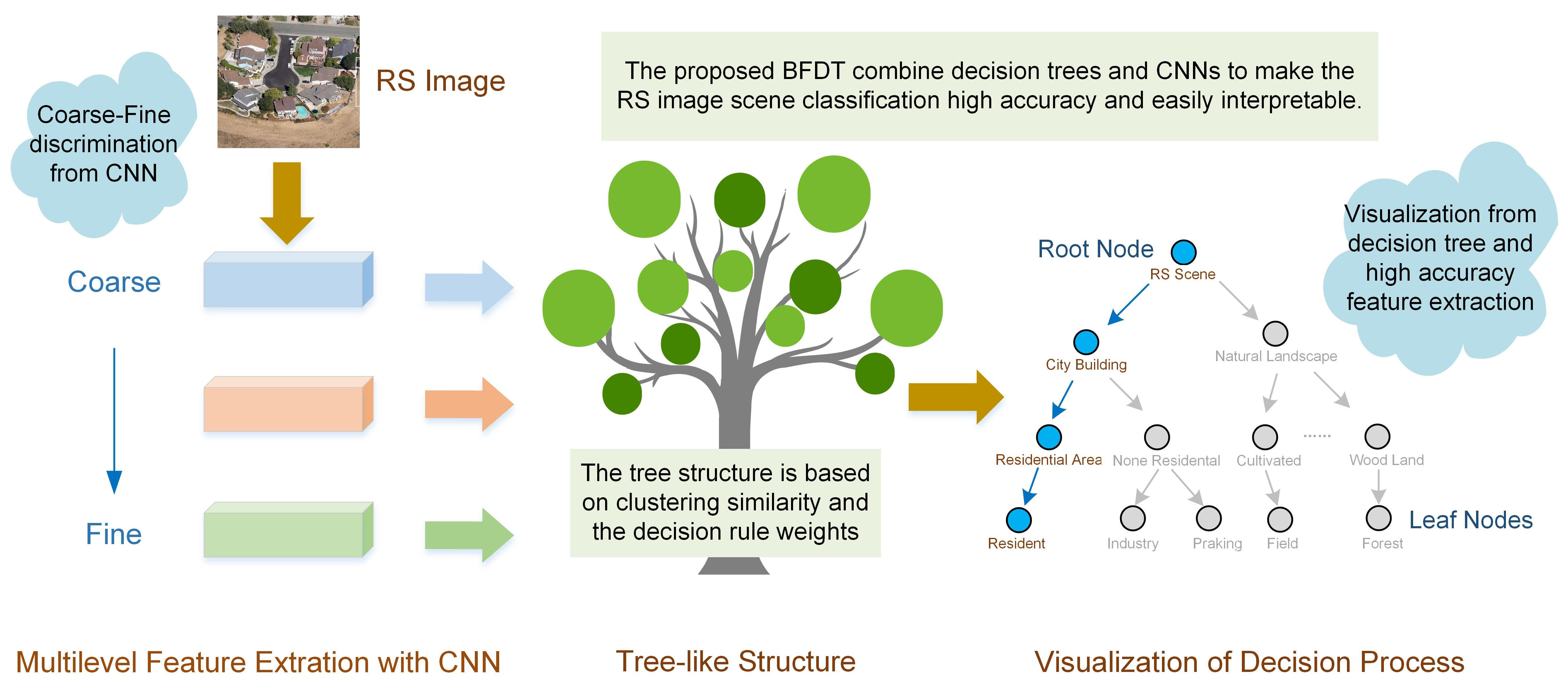
3.1. Overall Architecture

The BFDT algorithm determines a pretrained CNN architecture that utilizes the dependency structure of a DT trained on the RS image dataset. The proposed algorithm consists of the following three stages: (1) feature extraction, (2) decision process and (3) embedding decision rules (Figure 1). The BFDT adaptively fuses the direct inference along with top-down and bottom-up information for RSISC, leading to a bidirectional flow decision model. We begin by featuring each image sample using the pretrained CNN backbone, such as ResNet-18, ResNet-50 and AlexNet. Specifically, we use three separate public RS scene datasets to fine-tune the model’s weight. In addition, we use the last fully connected layer to build induced hierarchies. Moreover, decision nodes are labeled with RS expert knowledge and fine-tuned with a loss function.

3.2. Feature Extraction

Most CNN models are trained to make decision-making procedures in a coarse-to-fine way. Figure 2 shows that the extracted features become increasingly distinguishable at various levels. The low level cannot differentiate the final categories; they capture shallow features and obtain obvious visual cues to make coarse-grained and vague decisions. On the other hand, the high level is amenable to making the final classification, such as the features from the building categories tending to cluster.

For this purpose, we extract the features from the different layers of the pretrained CNN model to the decision tree via the regularization term. Supposing there are N categories in the RSISC task, each with M-associated samples for training, for the i-th level in the pretrained neural network, ${\mathrm{F}}_{\mathrm{m}}^{\mathrm{n}}\in {\mathrm{Z}}^{{\mathrm{w}}_i{\mathrm{h}}_i{\mathrm{c}}_i}$ denotes the features in the m-th image in the n-th classification category, where ${\mathrm{w}}_i$, ${\mathrm{h}}_i$, and ${\mathrm{c}}_i$ indicate the width, height, and channels of the feature map for the i-th level.

Because of the high feature dimensions and inconsistency at different levels, we use global average pooling with an adaptive filter size. Subsequently, we reduce the input and output data dimensions, i.e., ${\mathrm{F}}_{\mathrm{m}}^{\mathrm{n}}$ becomes a $c_i$-dimensional vector. After that, we further use Linear Discriminant Analysis (LDA) [61] to reduce the dimensions of features $\left(c_1,c_2,\dots \right)$ from different levels and compress them to a fixed scale $c \left(c\le c_1,c_2,\dots \right)$. The widely used dimensionality reduction methods include supervised approaches such as linear discriminant analysis (LDA) and unsupervised approaches such as principal component analysis (PCA) [62] In RSISC tasks, class labels are always available, and the supervised approaches such as LDA are usually more effective than unsupervised approaches such as PCA for classification. For this reason, we consider LDA to reduce the dimensions and preserve as much of the class discriminatory information as possible. It also utilizes the Fisher criterion that tackles the intraclass and interclass correlation. Inspired by the tree-like decision [27], we construct the intra-class scatter matrix $S_w$ for similar data and the inter-class scatter matrix $S_b$ for dissimilar data. The aim is to seek an optimal projection direction to maximize the interclass spread of distinct data and minimize the intraclass scatter of similar data. We define the Fisher criterion, which is maximized over all linear projections for each level $W$:

$$\mathcal{J}(W)=\arg {\max }_W\frac{W^T{S}_{b}W}{W^T{S}_{w}W}$$

(1)

The intra-class dispersion matrix $S_w$ and interclass dispersion matrix $S_b$ are defined as follows:

$$S_b={\displaystyle {\sum }_{i=1}^{N}M\cdot (\overline{f^n}-\overline{f})}{(\overline{f^n}-\overline{f})}^T$$

(2)

$$S_w={\displaystyle {\sum }_{i=1}^N{\displaystyle {\sum }_{m=1}^M(f_m^n-\overline{f^n}){(f_m^n-\overline{f^n})}^T}}$$

(3)

where $\overline{f^i}$ and $\overline{f}$ represent the averages of feature vectors from the i-th and all categories. Then, the corresponding categories are defined by averaging the feature vectors in the subspace. For clarity, a list of key symbols is shown in

Table 1. A list of symbols and descriptions.

Symbols	Descriptions
N	The categories in a dataset
${\mathrm{F}}_{\mathrm{m}}^{\mathrm{n}}$	The features extracted from the m-th image in the n-th classification category
$S_w$	The intraclass scatter matrix
$S_b$	The interclass scatter matrix
$\overline{f^i}$$, \overline{f}$	The averages of feature vectors from the i-th and all categories
M, N	N categories in the RSISC task, and each with M-associated training images
SSE	The sum of squared errors
$A_i,a_i$,	The i-th cluster and the cluster’s center
$v_i$	The i-th node in the decision tree
$w_i$	The weights of the node
$Y_{v_i}$	$\mathrm{The} \mathrm{category} \mathrm{contained} \mathrm{in} \mathrm{the} \mathrm{node} v_i$
L(i)	$\mathrm{The} \mathrm{path} \mathrm{from} \mathrm{the} \mathrm{root} \mathrm{to} \mathrm{the} \mathrm{node} v_i$
$p\left(L_n\left(i\right)|i\right)$	The probability that node i traverses to the next node on the path to class n
y	The ground truth labels

.

In the subspace, we adopt K-means to generate the tree-like similarity of categories and calculate the average feature vectors to represent the corresponding categories. The primary idea of clustering is to select K initial centroids based on a specific approach. The remaining data are then observed, and the clusters closest to the K points are divided using the Euclidean distance as the sample similarity measure. Finally, the centroids of each cluster are recalculated in the generated new clusters. To demonstrate the coarse-to-fine decision process underlying pretrained CNNs, we adopted k-means clustering with the evaluation score of the SSE (sum of squared errors).

As the number of clusters K increases, the sample division will be finer and the degree of aggregation of each cluster will gradually increase, i.e., the squared error and SSE will gradually decrease. When K is less than the optimal number of clusters, the decrease in SSE will be large because the increase in K will increase the degree of aggregation of each cluster significantly. When K reaches the optimal number of clusters, the degree of aggregation obtained by increasing K decreases rapidly, so the decline in SSE decreases abruptly, i.e., it tends to level off as the value of k continues to increase. In other words, the graph of SSE and k is the shape of an elbow, and the value of K corresponding to this elbow is the optimal number of clusters for the data. Figure 3 shows the SSE errors under the level-by-level ConvBlock. As shown in Figure 3a, the number of clusters is 2 at the elbow of the curve. It is defined as follows:

$$SSE={\displaystyle {\sum }_{i=1}^k{\displaystyle {\sum }_{(x\in A_i)}dist(a_i,x)}}$$

(4)

$$a_i=\frac{1}{sum}{\displaystyle \sum _{x\in A_i}x}$$

(5)

where $x$ represents the input sample, $A_i$ represents the i-th cluster, $a_i$ represents the cluster’s center, $sum$ is the number of input samples, and $dist(·)$ represents the Euclidean distance.

After k-means clustering, we construct a tree-like clustering similarity from training feature vectors. They are clustered at the first level with the number of centers equal to the initial centroids K. Each leaf node’s corresponding feature space partition is projected onto the two-dimensional space. Thus, at the successive levels, it will continue splitting feature vectors in each branch by the k-means until reaching the level.

3.3. Decision Rules and Process

As shown in Figure 2, hierarchical clustering separates each category, and it is difficult for users to understand what decision is made at each level. Therefore, the critical step of the BFDT algorithm is constructing the decision tree-based model. This can be a single decision tree from a single CNN. The tree depth is a hyperparameter that should be tuned for each RS image dataset. Our framework combines bottom-up and top-down information to build a hierarchical RSISC.

3.3.1. Generating the Decision Path

The decision tree is a coarse-to-fine decision process from the root node to the leaf nodes. The model makes the coarsest decision from the root node to its children. The most precise output should be reached when the leaf layer is reached. We use a graph $G=\left\{V,E\right\}$ to describe the DT, where $V=\left\{v_1,v_2,\dots \right\}$ is the node-set and $E=\left\{e_1,e_2,\dots \right\}$ is the edge set between the nodes. The number of leaf nodes is the number of categories, and each leaf node contains only one category, while the root node contains all categories. We use $Y_v$ to denote the category contained in node $v$. However, the intermediate layer only makes a rough classification. To embed the decision process of each layer into the decision tree, we use a top-down strategy to connect parent and child nodes. The distance between two nodes of adjacent layers is measured as follows:

$$D=dist(a_i,a_j)$$

(6)

where $a_i,a_j$ denote the center of the i-th cluster and j-th cluster, respectively. $dist(·)$ represents the Euclidean distance.

We obtain the distance D between the center of the upper cluster $A_i$ and the adjacent lower cluster $A_j$. If the lower node $v_j$ reaches the upper node $v_i$ at the closest distance, then node $v_j$ is regarded as the child of node $v_i$. Through this process, the categories contained in the intermediate nodes are determined. Finally, we add edges to the upper-level node $v_i$ and their children nodes$v_j$ to form an interpretable tree.

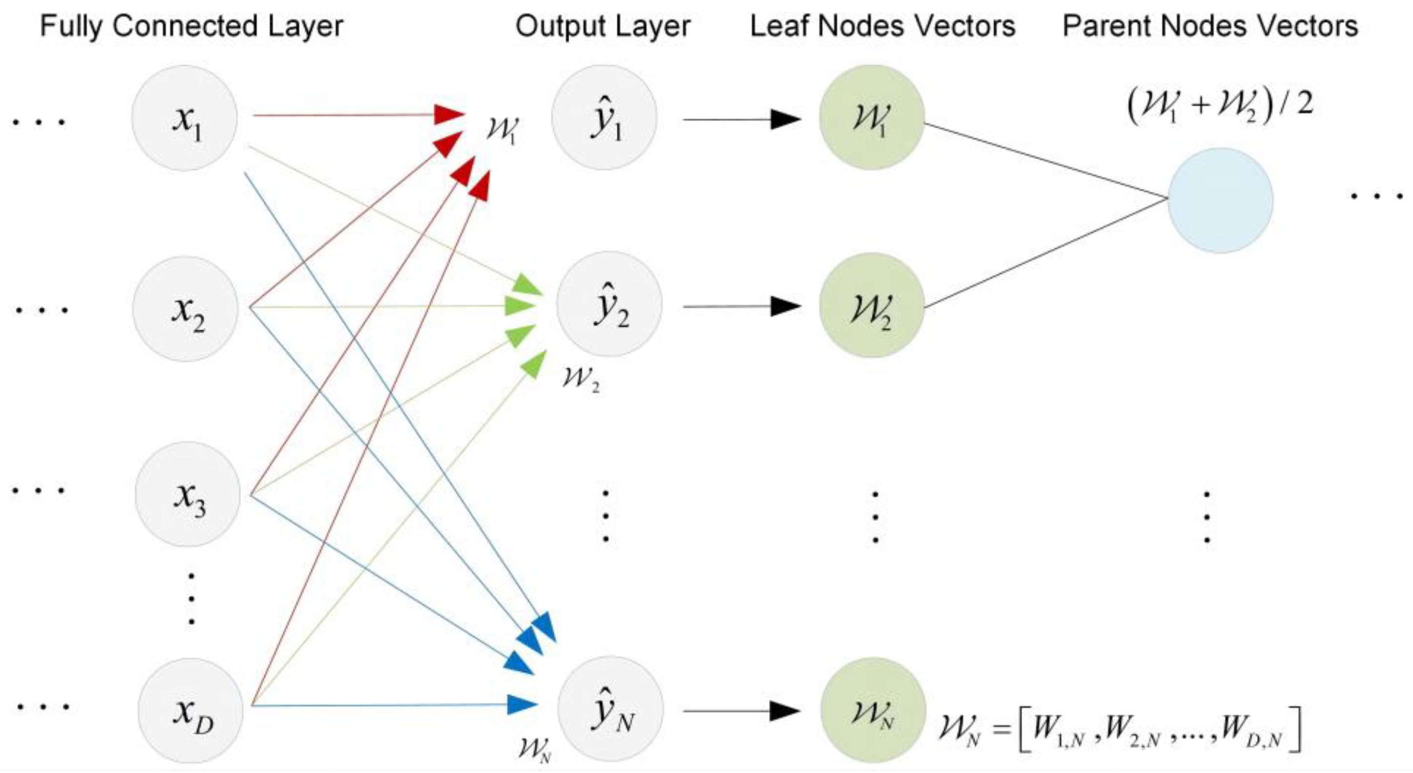
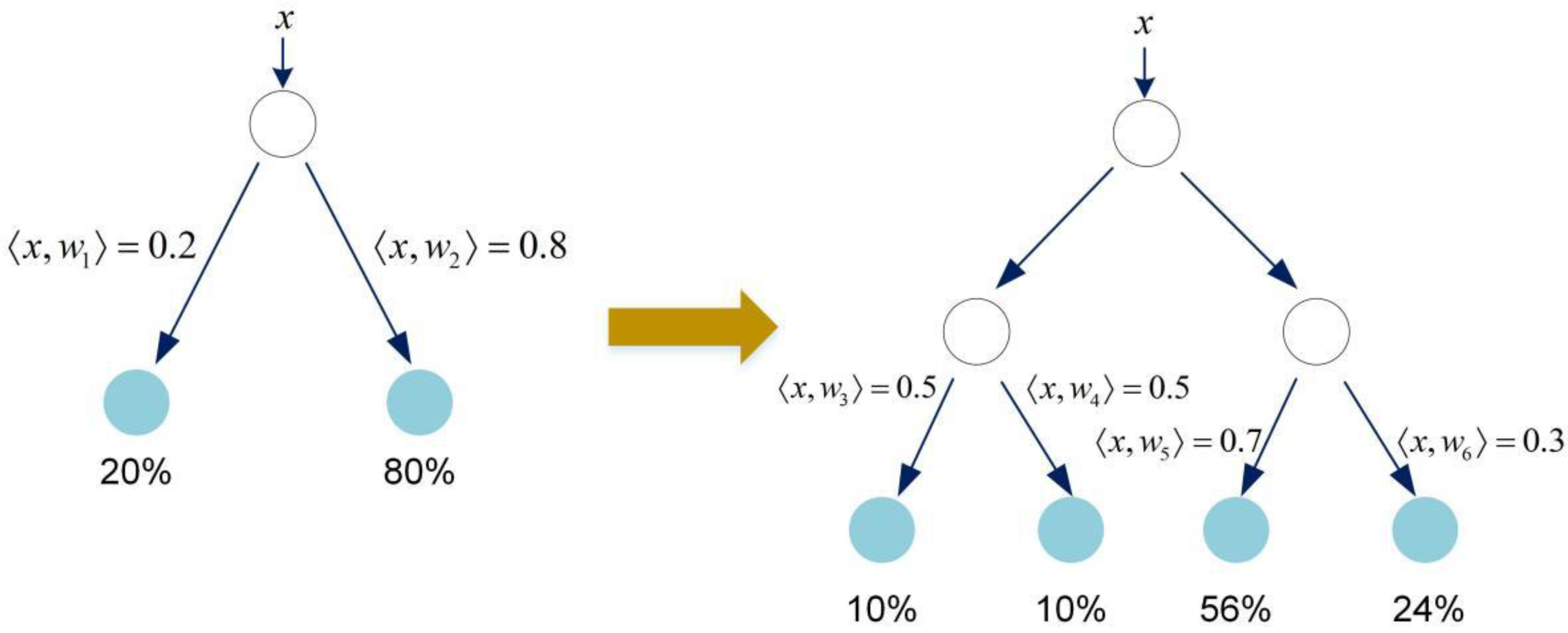
3.3.2. Decision Rule Weights

In this step, we adopt a bottom-up model to associate the weight space with each node. For the weight $𝓌\in {ℝ}^{D\times N}$ of a fully connected layer in the pretrained network, we select each row $𝓌{}_n\in 𝓌$ of the fully connected layer as the representative vector of the corresponding leaf node (Figure 4).

For each parent node in the decision tree, find all leaves $\mathrm{n}\in Y_{v_i}$ in the subtree of a node $v_i$ and average the weights of the nodes:

$$W_i=\frac{{\sum }_{k\in Y_{v_i}}{W}_k}{len\left(Y_{v_i}\right)}$$

(7)

3.3.3. Node Probabilities

Figure 5 shows sample $x$ traversing all intermediate nodes from top to bottom and calculating the inner product. The final probability of a leaf node is the product of the probabilities of each intermediate node on the path. Finally, the class to which $x$ belongs can be determined by comparing the magnitude of the final probability value on each leaf node. The softmax inner product calculates the probability between nodes. We compute the probability node $v_i$ with each child as:

$$S(j|i)=soft\max \left(\langle \overrightarrow{w_l},x\rangle \right)[j], \mathrm{where} \overrightarrow{w_l}={\left(\langle w_j,x\rangle \right)}_{j\in Y{v}_i}$$

(8)

where $x$ represents the input sample, $w_i$ represents the i-th weight, and $j$ represents the child of node $v_i$, $j\in Y_{v_i}$.

3.3.4. Leaf Picking

Consider the category n, which has a path from the root node to the leaf node. For a node $v_i$, we define the probability that it traverses path $L_n\left(i\right)$ to the next node as $p\left(L_n\left(i\right)|i\right)$. Then, the path probability $p\left(L_n\left(i\right)\right)$ of reaching a leaf node $v_k$ is denoted as:

$$S(n)={\displaystyle {\prod }_{i\in p_n}p(L_{n(i)}|i)}$$

(9)

The final class prediction is defined over these class probabilities

$$\stackrel{⌢}{n}=\arg {\max }_{n}p(n)=\arg {\max }_n{\displaystyle {\prod }_{i\in p_n}p(L_{n(i)}|i)}$$

(10)

3.3.5. Loss Function

When training CNNs with standard losses, they face the problems of dramatic data expansion, instability, and are not trained to separate representatives for each inner node. To address this issue, we propose cascaded softmax, which considers multilevel decision-making and measures the affinity between RS image scenes. At each decision level, the children nodes have a different granularity of similarity. In shallow features, information such as spatial texture works as a measure, while high-level semantics are used as the division principle in deep features. In other words, our cascading loss can be regarded as a soft constraint, where the penalty for misclassifying samples into different clusters is higher than belonging to the same cluster. The similarity measure between samples in the same cluster decreases, and the similarity measure between different clusters becomes larger, enabling the model to fully consider the intraclass and interclass relationships of the samples.

Intuitively, the tree-like supervised loss is particularly well suited to this work, where standard cross-entropy loss is not trained to separate representatives for each inner node. To address this, we make full use of both modes. The two components play different roles in the training process, with the tree-like loss focusing on improving top-1 accuracy and the other on improving the overall structure of the output space. They can complement each other well and avoid overfitting better, so we combine the standard loss with the tree supervised loss to calculate the mixed loss:

$$ℒ=CrossEntropy(({\alpha }_t{S}_{tree}(n)+{\beta }_t{S}_{s\tan dard}(n)),y_n)$$

(11)

where $S_{s\tan dard}(n)$ is the standard score of the n-th category, $S_{tree}(n)$ is the tree score, $\alpha$ and $\beta$ represent the varying weights, and y is the ground truth label.

In summary, our strategy has two benefits: (1) The bottom-up embedded decision rule model substitutes the data size limitation in the derivation process from root nodes to leaf nodes in previous methods. (2) The model directly uses the fully connected layer, maintaining the end-to-end high-performance advantage of the neural network.

3.4. Learning Procedure

BFDT-Train (Algorithm 1) learns a BFDT classifier from training samples. The algorithm begins by performing the train-prune-retrain process to update the parameters by maximizing Equation (1). It then computes the node probabilities and returns an oblique decision tree by employing the hierarchical loss of Equation (11).

Algorithm 1 BFDT Train

Input: RS Image Samples, Pre-trained CNN, T (a pre-defined hierarchy structure) Output: An BFDT model. 1:   Let K be the number of samples and l indicate the level index; 2:   for each l-th level in pretrained CNN do 3:     for each image sample k ∈ {1, …, K} do 4:      Adopt GAP to squeeze out the spatial dimensions. 5:     end for 6:     Adopt LDA to reduce dimension. 7:     Update W, Sb, Sw by maximizing Equation (1). 8:   end for 9:   for each row in T do 10:    Project all original features to the lower-dimensional subspace. 11:    Generate nodes with k-means by Equations (4)–(6). 12:    Seed decision rule weights from the pretrained CNN by Equation (7). 13:    Compute node probabilities by Equation (8). 14:  end for 15:  Fine-tuning the BFDT model with tree supervision loss by Equation (11).

4. Experimental Results

4.1. Datasets

We perform experimental evaluations on three public RS scene datasets, and their characteristics are shown in

Table 2. A detailed description of three datasets in the experiments.

Datasets	Number of Scene Classes	Number of Samples per Class	Total Number of Images	Spatial Resolution	Image Size
RSSCN7	7	400	2800	-	400 × 400
AID	30	200–400	10,000	0.5–0.8	600 × 600
NWPU45	45	700	31,500	0.2–30	256 × 256

. These datasets are captured from different satellite sensors under different conditions and over diverse locations of the ground surface, including rich diversities across different datasets.

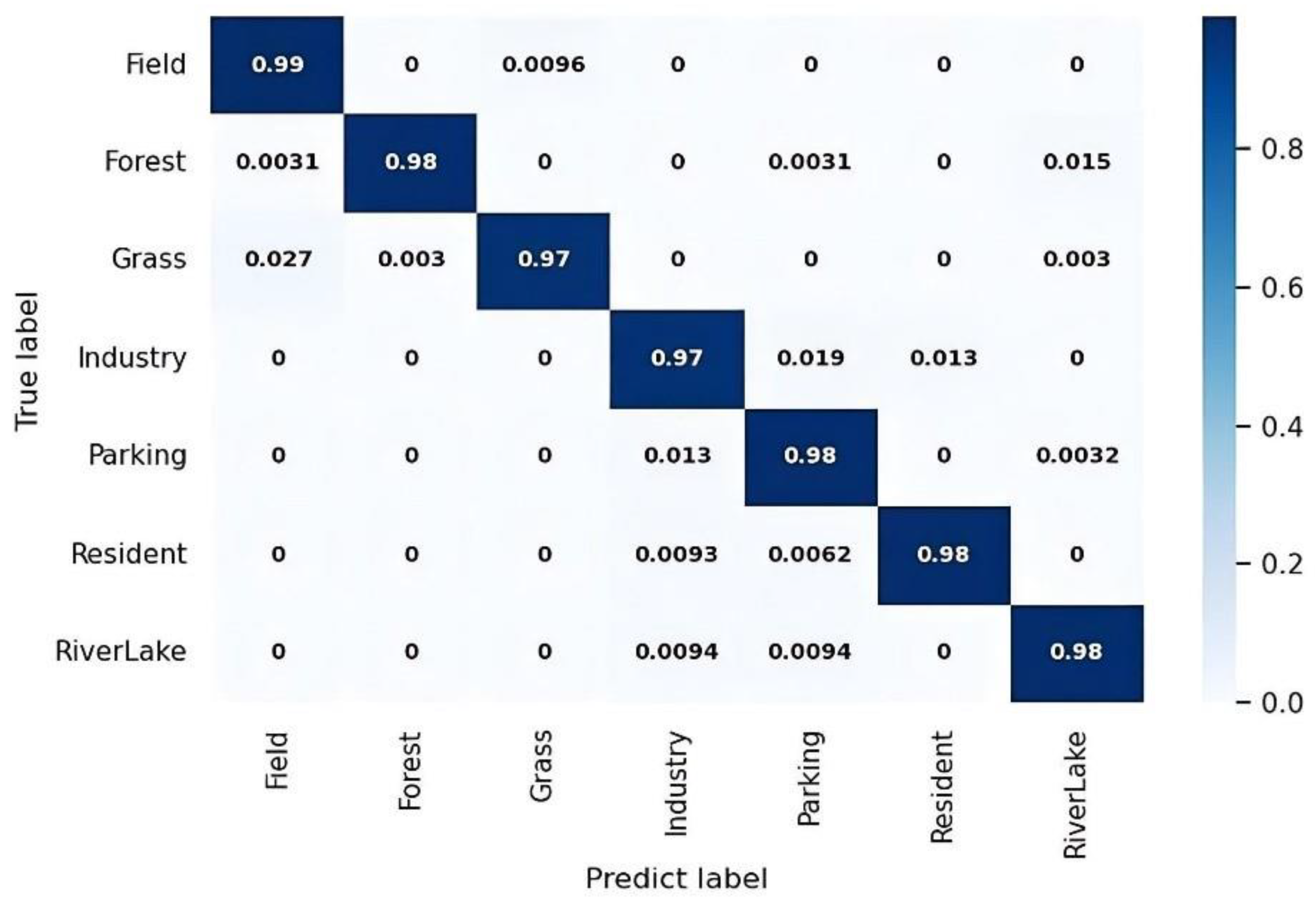
• RSSCN7: The RSSCN7 dataset [33] was established by Zou, Q et al. of Wuhan University in 2015. These images are from 7 specific scene categories: lakes, meadows, forests, farmland, lots, industrial areas, residential areas, and rivers and parking. Each scene consists of 400 images of 400 × 400 pixels, with four different scales for each category and 100 samples for each scale. Some sample images are shown in Figure 6. This paper uses training ratios of 20% and 50%, and the remaining values are used for testing.
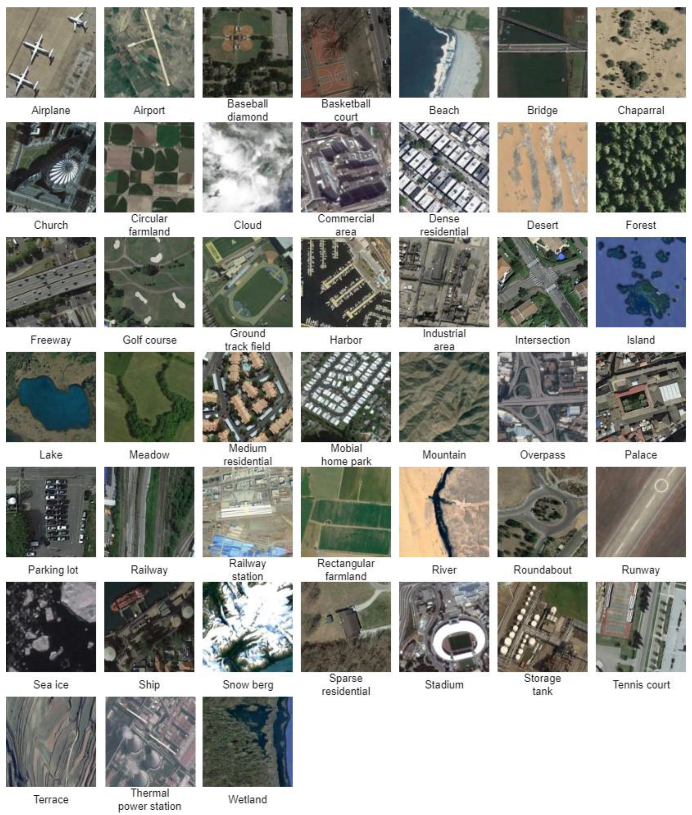
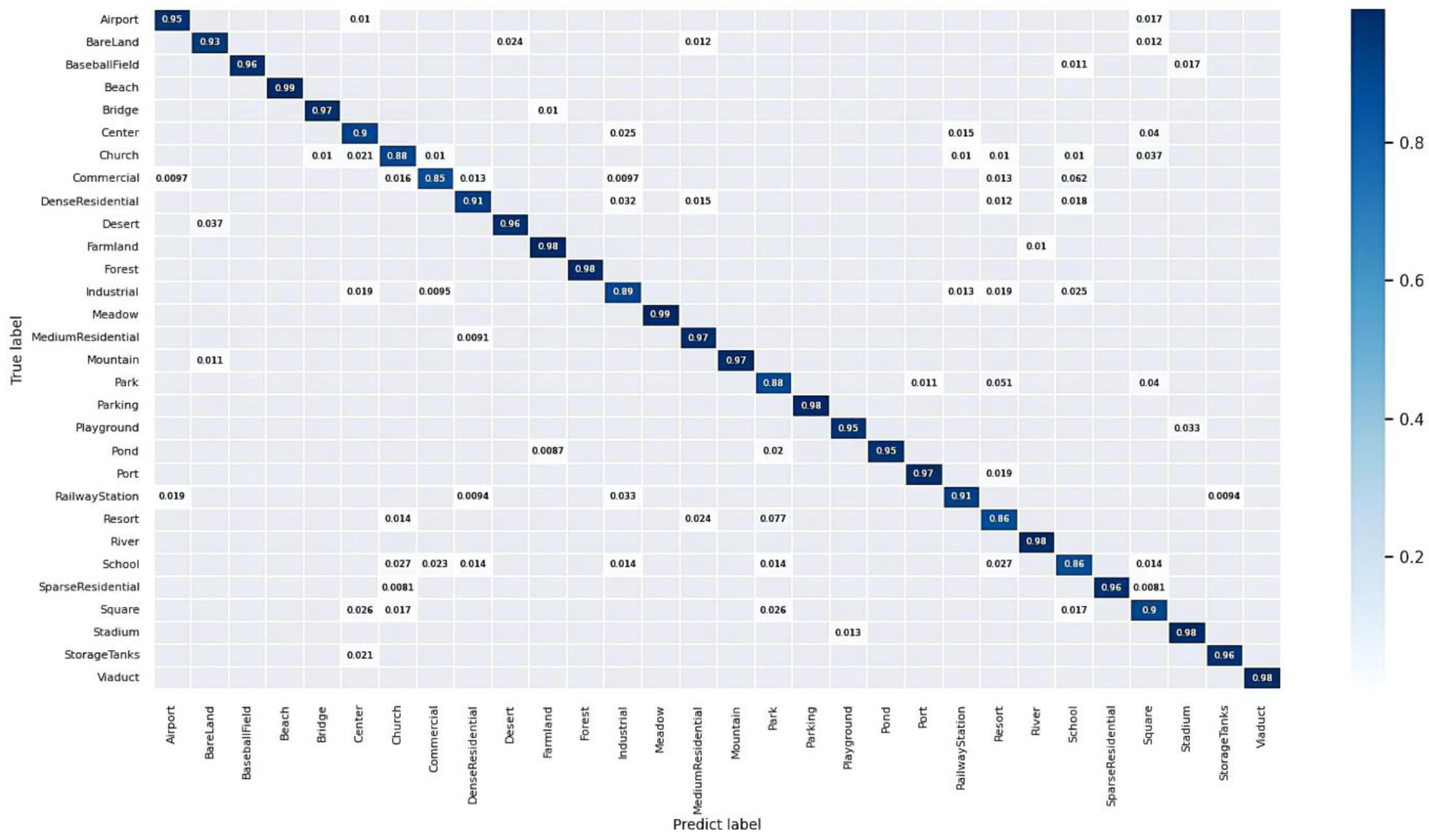
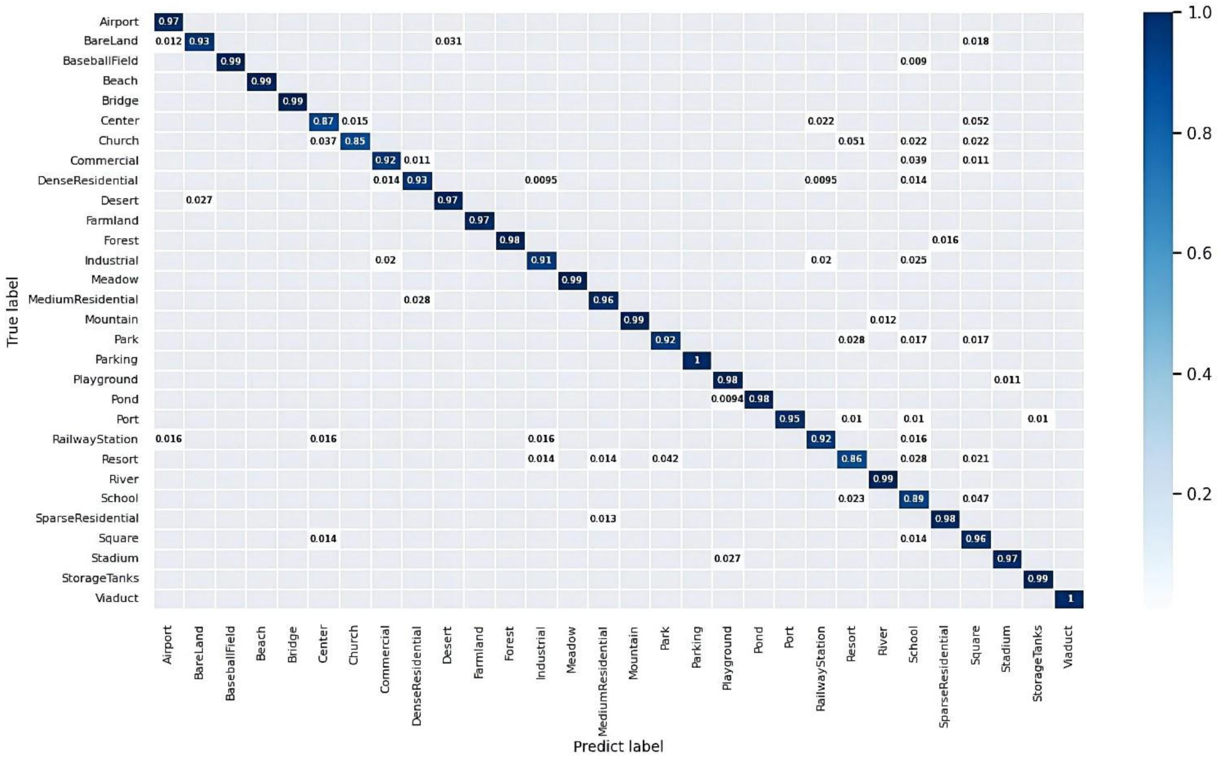
• AID: The Aerial Image dataset [34] was established by Xia et al. of Wuhan University in 2017, cropped and corrected at 600 × 600 pixels from Google Earth imagery. The dataset consists of 30 scenes with 200 to 400 images per class, and the spatial resolution of each class ranges from 0.8 m to 0.5 m. Some sample images are shown in Figure 7. As above, 20% and 50% are used as the training ratios, and the rest are used as tests.
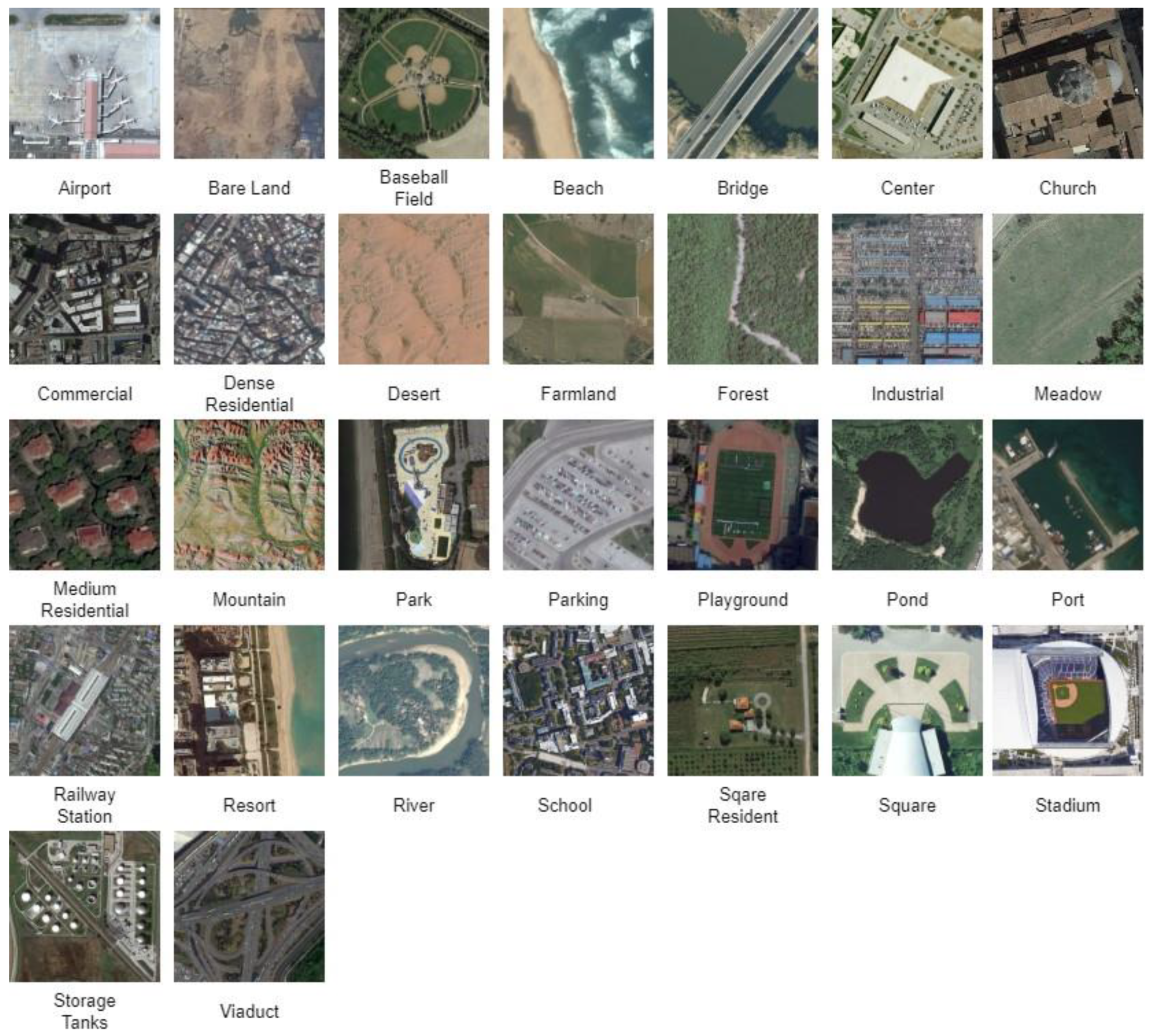
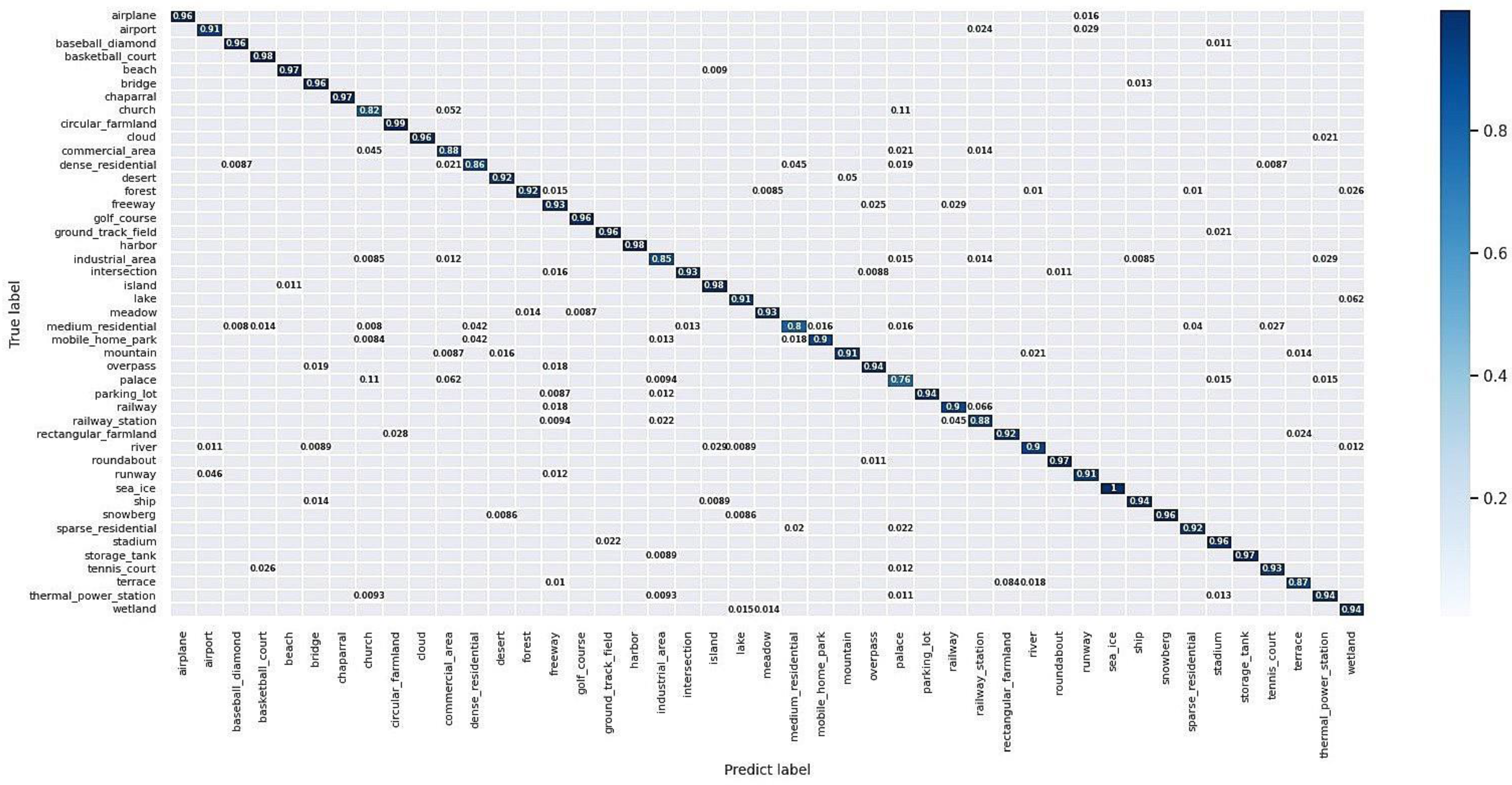
• NWPU: The NWPU-RESISC45 dataset [35] was published by Northwestern Polytechnic University and was obtained from Google Earth. The dataset comprises 45 scenes with 700 images per scene, totaling 31,500 samples. The image size is 256 × 256, and the pixel resolution varies from 30 to 0.2 m. This dataset is the largest in scene classes and the total number of images. Therefore, it contains richer image variation, greater internal diversity, and higher interclass similarity than the other datasets considered. Some sample images are shown in Figure 8. We utilize the training ratio of 20% and the remaining 80% as test data.

4.2. Evaluation Metrics

We evaluate remote sensing scene classification using the overall accuracy (OA) and confusion matrix (CM).

• Overall accuracy represents the ratio of correctly classified samples in the test set to the total number of samples and demonstrates the classification performance of the entire test dataset. It is common to see how well a scene classification method works in RS images.
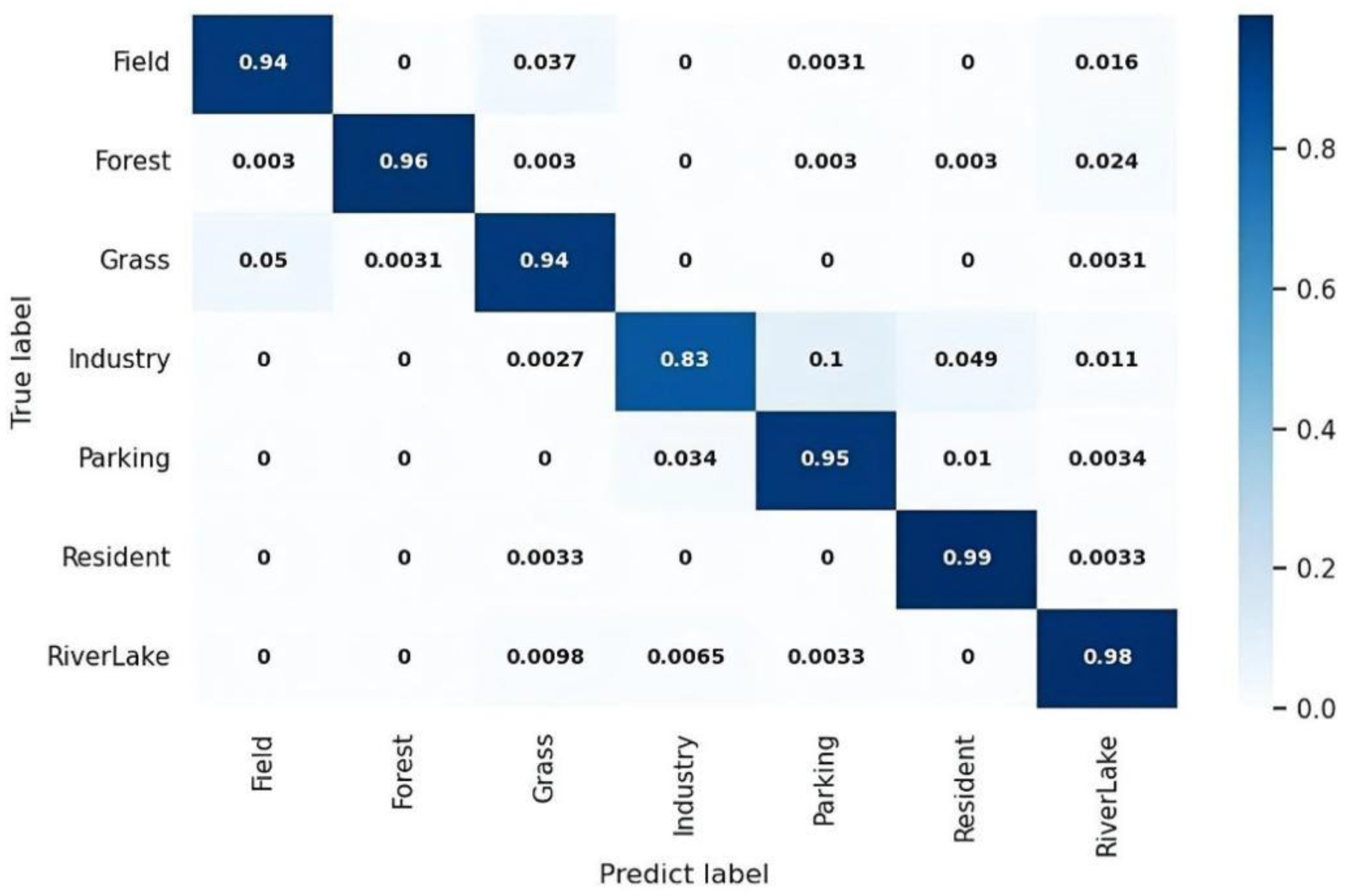
• The confusion matrix visualizes and summarizes the performance of a classification algorithm. It is an N × N squared matrix where N denotes the number of classes under consideration. Note that we used the normalized values and that the values on each row sum up to 1.

4.3. Experimental Settings

All experiments are implemented with the open-source library PyTorch. We use ResNet-18, ResNet-50 and AlexNet as the backbones. For multiple feature extraction layers, we use 5, 13 and the last Conv layer in ResNet-18; in ResNet-50, we use 22, 40, and the last Conv layer; in AlexNet, we use 2, 4, and the last Conv layer. Note that here we do not train the networks from scratch. In contrast, we use backbone networks pre-trained on ImageNet and fine-tuning them on the three RS datasets. The Adam optimizer is employed while the momentum is set to 0.7, and the learning rate is initialized to 1 × 10⁻⁴. We set the input size to 224 × 224 and used random horizontal flipping to enhance the image. The implementations are conducted on the Canonical Ubuntu 18.04 system equipped with an Nvidia Corp., Santa Clara, CA, USA, GeForce RTX 3080 GPU and Intel Corp., Santa Clara, CA, USA, i9-10920x CPU.

4.4. The Performance of the Proposed Method

The RS images from different datasets are collected by different sensors and over diverse locations of the ground surface, resulting in significant discrepancies in semantic information between different databases. In addition, various experts annotate different datasets, and the same scene from different datasets may be labeled with other class names. Our work aims to search for a network architecture with satisfactory accuracy and explainability. As a result, we further evaluated the proposed model for performance analysis on three datasets separately. The state-of-the-art RSISC methods based on DNNs were compared, including various classifiers and architectures. In particular, ResNet-18, ResNet-50 and AlexNet were used as the backbone networks to evaluate the relevance of the network depth and accuracy.

Table 3. Dataset training and testing ratio for three datasets in the experiments.

Datasets	Train	Test
RSSCN7	20%/50%	80%/50%
AID	20%/50%	80%/50%
NWPU45	20%	80%

shows the dataset’s training and testing proportions, which is the proportion of training samples to the total samples of the dataset.

4.4.1. Results on RSSCN7

We followed the training ratios proposed by [36].

Table 4. Performance comparison results with different state-of-the-art methods of OA on the RSSCN7 dataset under training ratios of 20% and 50%.

Methods	Year	Training Ratio
		20%	50%
TEX-Net-LF [36]	2018	92.45 ± 0.45	94.0 ± 0.57
Fine-tune MobileNet V2 [41]	2019	89.04 ± 0.17	92.46 ± 0.66
SE-MDPMNet [41]	2019	92.65 ± 0.13	94.71 ± 0.15
Dual Attention-aware features [47]	2020	91.07 ± 0.65	93.25 ± 0.28
LCNN-BFF [48]	2020	-	94.64 ± 0.21
Contourlet CNN [46]	2020	-	95.54 ± 0.71
ResNet18 (global + local) [43]	2020	93.89 ± 0.52	96.04 ± 0.68
CGDSN [49]	2021	-	95.46 ± 0.18
DLFP [45]	2021	-	95.49 ± 0.55
GLNet (VGG) [44]	2021	-	95.07
GeoKR(ResNet50) [50]	2021	89.33	91.52
EfficientNetB3-Basic [42]	2021	92.06 ± 0.39	94.39 ± 0.10
EfficientNetB3-Attn-2 [42]	2021	93.30 ± 0.19	96.17 ± 0.23
LNR-ResNet50 [51]	2022	-	96.8 ± 0.32
BDFT (ResNet50)	2022	94.11	96.50
BDFT (AlexNet)	2022	92.71	93.54
BDFT (ResNet18)	2022	95.15 ± 0.41	97.05 ± 0.35

compares the proposed model with some state-of-the-art methods in recent years on RSSCN7 datasets. The algorithm reaches 95.15% and 97.05% accuracy for remote sensing image scene classification, outperforming all comparative methods. With a training ratio of 20%, our method is 2.7% higher than TEX-Net-LF [36], 2.5% higher than SE-MDPMNet [41], 1.85% higher than EfficientNetB3-Attn-2 [42], and 1.26% higher than global-local dual-stream networks (ResNet18 (global + local)) [43]. With a training ratio of 50%, our method is 2.34% higher than SE-MDPMNet [41], 1.98% higher than GLNet (VGG) [44], 1.56% higher than multilayer feature decision-level fusion (DLFP) [45], 1.51% higher than the multidilation pooling module Contourlet CNN [46], and 1.01% higher than global-local dual-stream networks (ResNet18 (global + local)) [43]. The results show that our method achieves the best classification accuracy regardless of the training ratio. From the tables, we can observe that ResNet achieves better performance in our method than the feature maps of AlexNet. Intuitively, the difference is caused by the depths of different models. AlexNet has just five convolutional layers, ResNet-18 has 17 convolutional layers, and ResNet-50 has 49 convolutional layers. However, the classification accuracy for ResNet18 as the backbone is still better than that of ResNet-50. This indicates that the depth of the backbone DNNs does not determine the classification accuracy in this strategy. In this case, the latent variable “level” also played an important role in the overall framework.

An overview of the performance of BFDT is shown in the confusion matrix in Figure 9 and Figure 10. All of the scene categories can be fully recognized by BFDT, except for the industry scene; there is some confusion between the parking and industry scenes. This may be because the two categories are a mixture of pavement cover and car. For the RSSCN7 dataset, we conduct a detailed performance analysis of the proposed model adopting the confusion matrix, and the results are shown in Figure 9 and Figure 10. When the training sample is 20%, except for the Industry category, the accuracy rate can reach more than 90%. When the training sample is 50%, the classification accuracy of all scenarios is higher than 97%. Overall, the classification accuracy of “Industry” scenes is the lowest at both training ratios, 83% and 97%, respectively. Mainly due to the extreme similarity between “parking” and “Industry”, some are incorrectly classified as “parking”.

4.4.2. Results on AID

We followed the training ratios proposed by [36].

Table 5. Performance comparison of different methods of OA on the AID dataset under a training ratios of 20% and 50%.

Methods	Year	Training Ratio
		20%	50%
TEX-Net-LF [36]	2018	93.81 ± 0.12	95.73 ± 0.0.16
ARCNet-VGG16 [40]	2019	88.75 ± 0.40	93.10 ± 0.55
SCCov [52]	2019	93.12 ± 0.25	96.10 ± 0.16
CNN-CapsNet [38]	2019	93.60 ± 0.12	96.66 ± 0.11
Dual Attention-aware [47]	2020	94.36 ± 0.54	95.53 ± 0.30
Contourlet CNN [46]	2020	-	95.54 ± 0.71
ResNet18(global + local) [43]	2020	93.89 ± 0.52	96.04 ± 0.68
VGG-VD16 [53]	2020	94.75 ± 0.23	96.93 ± 0.16
EfficientNetB3-Attn-2 [42]	2021	94.45 ± 0.76	96.56 ± 0.12
LCNN-CMGF [54]	2021	93.63 ± 0.1	97.54 ± 0.25
D-CNN [55]	2021	94.63	96.43
DLFP [45]	2021	94.69 ± 0.23	96.67 ± 0.28
MSA-Network [39]	2021	93.53 ± 0.21	96.01 ± 0.43
LGRIN [19]	2021	94.74 ± 0.23	97.65 ± 0.25
RANet [37]	2021	92.71 ± 0.14	95.31 ± 0.37
GRMA-Net-ResNet18 [56]	2021	94.58 ± 0.25	97.05 ± 0.37
BDFT (ResNet50)	2022	94.85	96.88
BDFT (AlexNet)	2022	86.60	91.98
BDFT (ResNet18)	2022	95.05 ± 0.49	97.76 ± 0.87

compares the proposed model with some state-of-the-art methods in recent years on AID datasets. The algorithm reaches 95.05% and 97.76% accuracy for remote sensing image scene classification, outperforming all comparative methods. With a training ratio of 20%, our method is 2.34% higher than RANet [37], 1.99% higher than CNN-CapsNet [38], 1.52% higher than MSA-Network [39], 1.24% higher than TEX-Net-LF [36], and 1.16% higher than global-local dual-stream networks (ResNet18 (global + local)) [43]. With a training ratio of 50%, our method is 4.66% higher than ARCNet-VGG16 [40], 2.22% higher than multidilation pooling module Contourlet CNN [46], 2.03% higher than TEX-Net-LF [36], 1.75% higher than MSA-Network [39], 1.72% higher than global-local dual-stream networks (ResNet18 (global + local)) [43], and 1.09% higher than multilayer feature decision-level fusion (DLFP) [45]. The results show that our method achieves the best classification accuracy regardless of the training ratio. Compared with using ResNet50 and AlexNet, the classification accuracy for ResNet18 as the backbone is still the best.

Then, the confusion matrix with 20% and 50% training ratios is displayed in Figure 11 and Figure 12. When the training sample is 20%, 24 scene categories have an accuracy higher than 90% among the 30 categories in the AID dataset. When the training ratio is 50%, 20 scene categories can reach more than 95%, and the classification accuracy of “Parking” and “Viaduct” is 100%. Among the misclassified samples, “Resort” accounted for a considerable percentage. Some are incorrectly classified as “Park” because both the “Resort” and “Park” samples have trees, water, and sparse buildings, making them difficult to distinguish and resulting in poor classification.

4.4.3. Results on NWPU-RESISC45

To keep pace with the compared method on NWPU-RESISC45, we set a training ratio of 20%.

Table 6. Performance comparison of different methods of OA on the NWPU-RESISC45 dataset under a training ratio of 20%.

Methods	Year	OA (%)
Discriminative + AlexNet [57]	2018	87.24 ± 0.12
ADSSM [13]	2018	94.29 ± 0.14
RD [60]	2019	91.03
VGG-16-CapsNet [38]	2019	89.18 ± 0.14
Contourlet CNN [46]	2020	89.57 ± 0.45
Hydra (DenseNet + ResNet) [14]	2019	94.51 ± 0.21
Hydra (ResNet) [14]	2019	91.96 ± 0.71
MG-CAP with Biliner [58]	2020	91.72 ± 0.16
EfficientNet [63]	2020	81.83 ± 0.15
LCNN-BFF [48]	2020	91.73 ± 0.17
ResNet18(global + local) [43]	2020	92.79 ± 0.11
VGG_VD16 with SAFF [64]	2020	87.86 ± 0.14
MobileNetV2-SCS [59]	2021	91.17
ResNet50-SCS [59]	2021	91.83
ResNet101-SCS [59]	2021	91.91
VGG-19-0.3 [65]	2021	90.19
AMB-CNN [66]	2021	92.42
BDFT (AlexNet)	2022	86.44
BDFT (ResNet50)	2022	94.07
BDFT (ResNet18)	2022	92.83 ± 0.11

compares the proposed model with some state-of-the-art methods in recent years on the NWPU-45 datasets. With 20% of training samples, the algorithm reaches 94.07% accuracy for RSISC, which is 6.83% higher than Discriminative + AlexNet [57], 4.89% higher than CNN-CapsNet [38], 2.35% higher than MG-CAP with Biliner [58], 2.90% higher than MobileNetV2-SCS [59] and 4.50% higher than Contourlet CNN [46]. The classification accuracy of BFDT with ResNet50 is very close to the classification accuracy of ADSSM [13] and Hydra (DenseNet + ResNet) [14], which is better than Hydra with ResNet-50. To obtain a similar performance, Hydra uses two CNN architectures, ADSSM combines sparse topics and deep features with late fusion, and the construction of our method is simpler. Regarding computational resource consumption, BFDT has some advantages compared to state-of-the-art classifiers.

Then, we conduct a detailed performance analysis of the proposed model adopting the confusion matrix, and the result is shown in Figure 13. Among the 45 categories in the NWPU-RESISC45 dataset, the accuracy of 37 scene categories can reach more than 90%. Among the misclassified samples, “Palace” accounted for the most significant percentage. Some are incorrectly classified as “Church” because both the “Palace” and “Church” samples have the same spatial layout and similar color distribution, making them difficult to distinguish and resulting in poor classification.

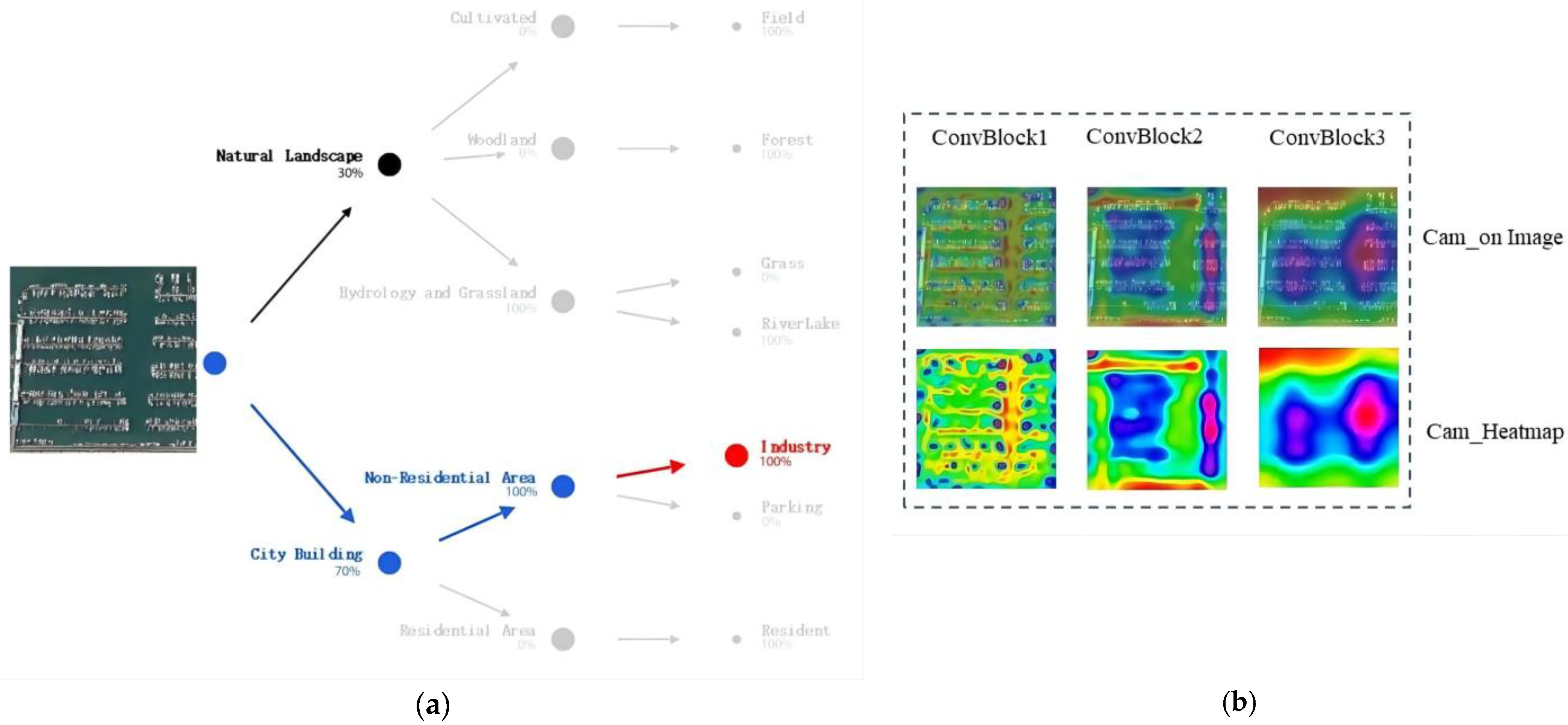
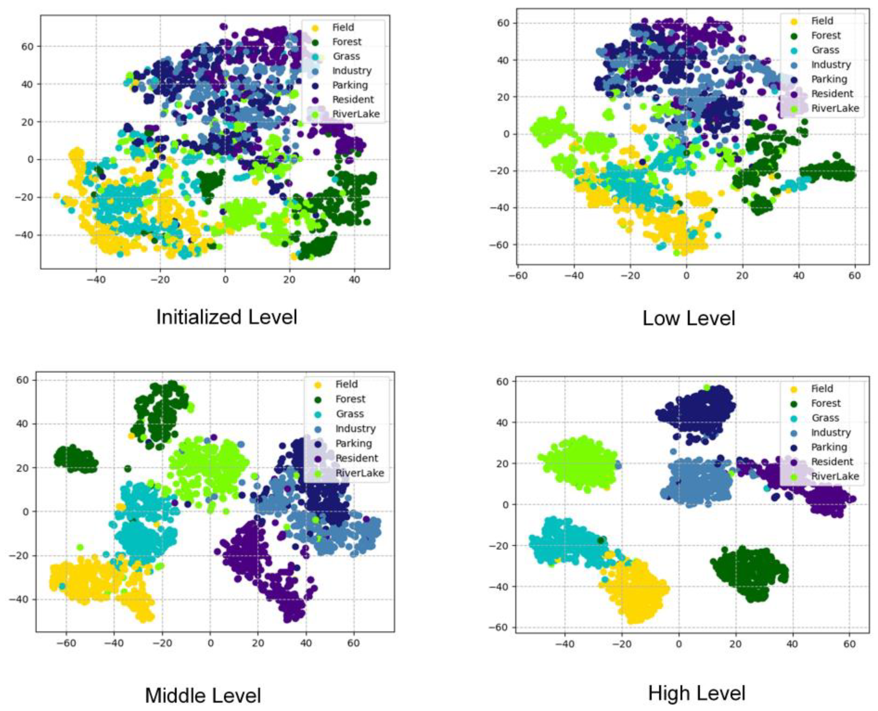
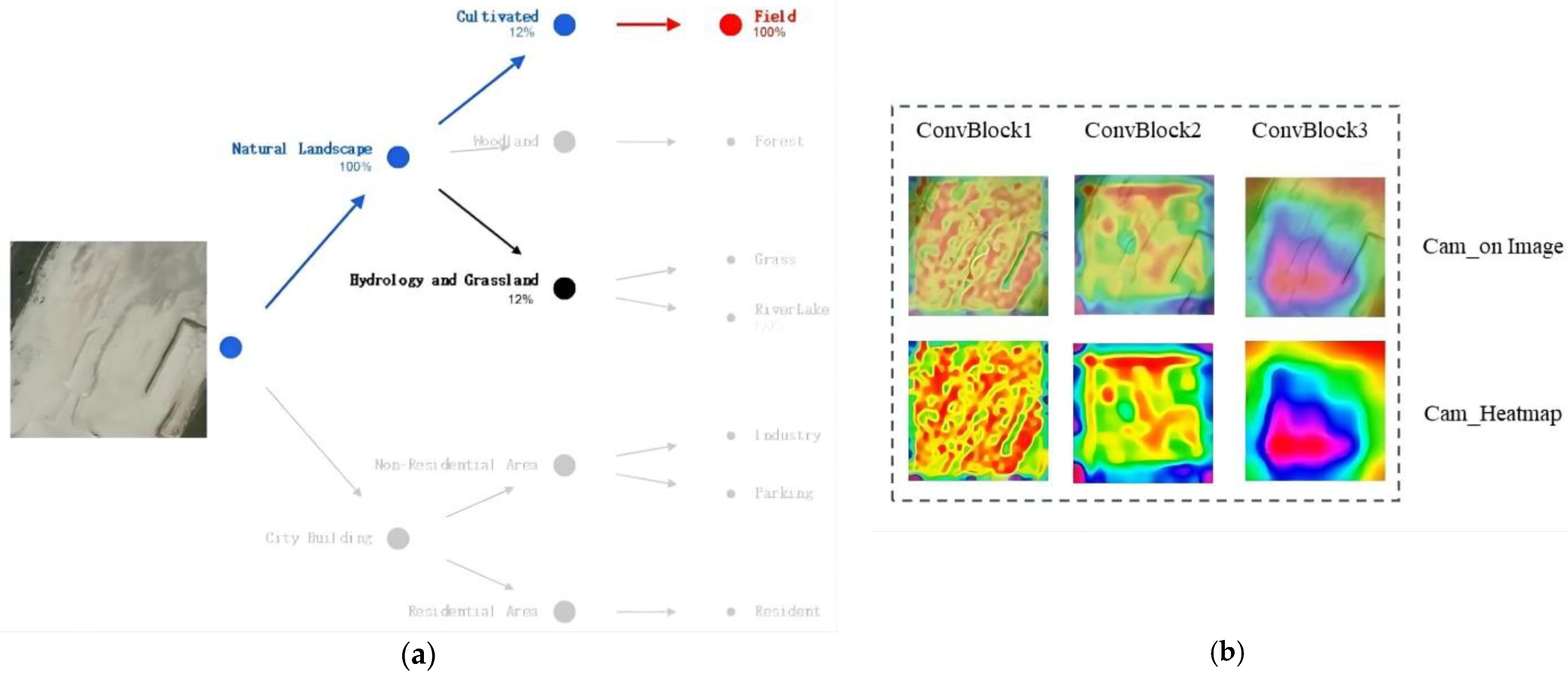
4.5. Reliability with Tree Traversal

The so-called “big data” era has increasing potential for RSISC. However, the gap between a finite class of labels and an infinite class of realistic scenarios makes the model critically generalizable. In our study, we define superclasses as the parents of several categories. (e.g., the nonresidential area is a superclass of parking and industry). Inspired by [67], we find that unseen classes from other datasets belong to the same superclass; for example, Pull BareLand and Port images from the AID dataset. The key to unseen scenes is that they are classified as the correct superclass; for example, make sure BareLand is classified as Natural Landscape). Recent advances in explainable DL can be grouped into saliency maps and ordered decision processes. The former explains model predictions by identifying which pixels most affected the forecast. However, by focusing on the input, saliency maps fail to capture the model’s decision-making process. From a practical perspective, explanations are essential for RSISC users to understand and trust the decision process. Therefore, there is a need to develop methods that provide a reliable decision process and, by doing so, to make models correctable and eventually trustworthy for predictions and design tasks.

We visualize the decision path on AID to demonstrate the process underlying pretrained models. There are several classes of AID, which are unseen classes for RSSCN7. Figure 14a and Figure 15a show that our model making decisions between equal likelihood classes will have lower certainty. Other choices have a high degree of certainty. The Port scene has the background of a natural landscape but also assumes the function of city buildings, so the accuracy of the two will be slightly lower compared to each other. In contrast, the functional attributes of the port are more robust than the presence of the background, so the port is more inclined to city building (Natural Landscape 30%, City Building 70%). However, as shown in Figure 14b and Figure 15b, the CAM diagram only gives the area of concern for each convblock and does not provide assistance to the decision-making process.

A fundamental element of the demand for explainability is the explanation of what the system is trying to achieve. The proposed approach decomposed the RSISC task into a sequence of decisions without human intervention in the decision process, which provides a structure to systematically integrate disparate components and correlations among data and causality between variables. For example, in Figure 15, the root note differentiates between city buildings and natural landscapes. These results also validate that although the low-level layers cannot make accurate predictions, they can differentiate between coarser-grained categories.

5. Discussion

Recent deep learning approaches have primarily focused on big data, but for many RSISC applications, samples are insufficient and spatially correlated with various noise. The DT is a classic machine learning method for classification. It is well understood and interpretable, but the classification effect is strongly affected by the size of the dataset. In contrast, CNN exhibits high performance but is opaque in explainability. In this work, we adopted a decision tree structure to maintain interpretability while preserving competitive reliability, with the results shown in Table 4, Table 5 and Table 6. In such a case, the bidirectional feature-flow mode enhances model interpretability. Previous methods used the bottom-up embedded approach from root to leaf nodes in derivation. In contrast, we combine the unique properties of RS images to construct a cascade loss, using the discriminative properties of various layers to improve the reliability.

We focus on RSISC decision-making using tree-based algorithms that learn the relationships between data inputs and decision outputs. Taking explainability as the demand for RSISC, the aim is that it could lead to human-like decisions. Significantly, the BFDT algorithm maps an ensemble of neural networks into an initialized DT ensemble. The powerful capabilities of CNNs are combined with DT models to create explainable and accurate approaches. The information mapped from the last layer into initial weights provides a user-friendly start to the DT training process because the deeper convolutional layer in the CNNs is more inclined to mine deeper information, for example, global feature information.

6. Conclusions

In this work, we described BFDT, a new approach for RSISC. In addition to reliability, it also preserves competitive accuracy. The primary significance of decision trees is that they provide the results and the decision process, which is a side effect of the way humans mind when making inferences. Specifically, we adopt a pretrained CNN model to construct the tree structure by parsing layer by layer through a top-down model. Meanwhile, the bottom-up model circumvents the overfitting defect caused by the branch structure of the traditional tree structure and fully guarantees the classification performance. Finally, we constructed the cascading softmax loss to compensate for the neglected interclass relationships by exploiting the rich interlayer relationships in the tree structure. Due to the unique tree structure, a specific reference value can be generated for unseen classes. We evaluate the proposed method on three mainstream RSI datasets, and the experimental results demonstrate the superior classification performance of our model compared to the state-of-the-art techniques. Extensive experiments show that our approach has higher accuracy, better interpretability, and stronger generalizability.

Explanations may be essential for users to understand and effectively manage RSISC tasks. However, every explanation within a context depends on the task and user expectations. Because the BFDT is compatible with various CNNs, the model could dynamically adapt to the non-stationary nature of scenes, which is the focus of our future work. From a human-centered perspective, research on competencies and knowledge could take explainable RSISC beyond explaining a decision procedure and helping its users determine appropriate trust. In the future, it may eventually have substantial roles, including learning and presenting to individuals and coordinating to connect knowledge. Moreover, CAM methods have been successful for explainable tasks, and incorporating these techniques into our proposed methods is an interesting direction for future work.

References

1. Zhang, L.; Zhang, L.; Du, B. Deep Learning for Remote Sensing Data: A Technical Tutorial on the State of the Art. IEEE Geosci. Remote Sens. Mag. 2016, 4, 22–40. [Google Scholar] [CrossRef]
2. Lv, Z.Y.; Shi, W.; Zhang, X.; Benediktsson, J.A. Landslide Inventory Mapping from Bitemporal High-Resolution Remote Sensing Images Using Change Detection and Multiscale Segmentation. IEEE J. Sel. Top. Appl. Earth Obs. Remote Sens. 2018, 11, 1520–1532. [Google Scholar] [CrossRef]
3. Longbotham, N.; Chaapel, C.; Bleiler, L.; Padwick, C.; Emery, W.J.; Pacifici, F. Very High Resolution Multiangle Urban Classification Analysis. IEEE Trans. Geosci. Remote Sens. 2012, 50, 1155–1170. [Google Scholar] [CrossRef]
4. Huang, X.; Wen, D.; Li, J.; Qin, R. Multi-Level Monitoring of Subtle Urban Changes for the Megacities of China Using High-Resolution Multi-View Satellite Imagery. Remote Sens. Environ. 2017, 196, 56–75. [Google Scholar] [CrossRef]
5. Lowe, D.G. Distinctive Image Features from Scale-Invariant Keypoints. Int. J. Comput. Vis. 2004, 60, 91–110. [Google Scholar] [CrossRef]
6. Risojević, V.; Babić, Z. Fusion of Global and Local Descriptors for Remote Sensing Image Classification. IEEE Geosci. Remote Sens. Lett. 2013, 10, 836–840. [Google Scholar] [CrossRef]
7. Ojala, T.; Pietikainen, M.; Maenpaa, T. Multiresolution Gray-Scale and Rotation Invariant Texture Classification with Local Binary Patterns. IEEE Trans. Pattern Anal. Mach. Intell. 2002, 24, 971–987. [Google Scholar] [CrossRef]
8. Dalal, N.; Triggs, B. Histograms of Oriented Gradients for Human Detection. In Proceedings of the 2005 IEEE Computer Society Conference on Computer Vision and Pattern Recognition (CVPR’05), San Diego, CA, USA, 20–25 June 2005; Volume 1, pp. 886–893. [Google Scholar]
9. Liu, N.; Wan, L.; Zhang, Y.; Zhou, T.; Huo, H.; Fang, T. Exploiting Convolutional Neural Networks with Deeply Local Description for Remote Sensing Image Classification. IEEE Access 2018, 6, 11215–11228. [Google Scholar] [CrossRef]
10. Boualleg, Y.; Farah, M.; Farah, I.R. Remote Sensing Scene Classification Using Convolutional Features and Deep Forest Classifier. IEEE Geosci. Remote Sens. Lett. 2019, 16, 1944–1948. [Google Scholar] [CrossRef]
11. Cheng, G.; Ma, C.; Zhou, P.; Yao, X.; Han, J. Scene Classification of High Resolution Remote Sensing Images Using Convolutional Neural Networks. In Proceedings of the 2016 IEEE International Geoscience and Remote Sensing Symposium (IGARSS), Beijing, China, 10–15 July 2016; pp. 767–770. [Google Scholar]
12. Hariharan, B.; Arbelaez, P.; Girshick, R.; Malik, J. Hypercolumns for Object Segmentation and Fine-Grained Localization. In Proceedings of the IEEE Conference on Computer Vision and Pattern Recognition (CVPR), Boston, MA, USA, 7–12 June 2015; pp. 447–456. [Google Scholar]
13. Zhu, Q.; Zhong, Y.; Zhang, L.; Li, D. Adaptive Deep Sparse Semantic Modeling Framework for High Spatial Resolution Image Scene Classification. IEEE Trans. Geosci. Remote Sens. 2018, 56, 6180–6195. [Google Scholar] [CrossRef]
14. Minetto, R.; Pamplona Segundo, M.; Sarkar, S. Hydra: An Ensemble of Convolutional Neural Networks for Geospatial Land Classification. IEEE Trans. Geosci. Remote Sens. 2019, 57, 6530–6541. [Google Scholar] [CrossRef]
15. He, N.; Fang, L.; Li, S.; Plaza, A.; Plaza, J. Remote Sensing Scene Classification Using Multilayer Stacked Covariance Pooling. IEEE Trans. Geosci. Remote Sens. 2018, 56, 6899–6910. [Google Scholar] [CrossRef]
16. Liu, Y.; Liu, Y.; Ding, L. Scene Classification Based on Two-Stage Deep Feature Fusion. IEEE Geosci. Remote Sens. Lett. 2018, 15, 183–186. [Google Scholar] [CrossRef]
17. Goel, A.; Banerjee, B.; Pižurica, A. Hierarchical Metric Learning for Optical Remote Sensing Scene Categorization. IEEE Geosci. Remote Sens. Lett. 2019, 16, 952–956. [Google Scholar] [CrossRef]
18. Zhang, X.; Tan, X.; Chen, G.; Zhu, K.; Liao, P.; Wang, T. Object-Based Classification Framework of Remote Sensing Images with Graph Convolutional Networks. IEEE Geosci. Remote Sens. Lett. 2022, 19, 8010905. [Google Scholar] [CrossRef]
19. Xu, C.; Zhu, G.; Shu, J. A Lightweight and Robust Lie Group-Convolutional Neural Networks Joint Representation for Remote Sensing Scene Classification. IEEE Trans. Geosci. Remote Sens. 2022, 60, 5501415. [Google Scholar] [CrossRef]
20. Huang, S.; Zhang, H.; Pižurica, A. Subspace Clustering for Hyperspectral Images via Dictionary Learning with Adaptive Regularization. IEEE Trans. Geosci. Remote Sens. 2022, 60, 5524017. [Google Scholar] [CrossRef]
21. Zhou, B.; Khosla, A.; Lapedriza, A.; Oliva, A.; Torralba, A. Learning Deep Features for Discriminative Localization. In Proceedings of the IEEE Conference on Computer Vision and Pattern Recognition (2016), Las Vegas, NV, USA, 27–30 June 2016; pp. 2921–2929. [Google Scholar]
22. Song, W.; Dai, S.; Wang, J.; Huang, D.; Liotta, A.; Di Fatta, G. Bi-Gradient Verification for Grad-CAM Towards Accurate Visual Explanation for Remote Sensing Images. In Proceedings of the 2019 International Conference on Data Mining Workshops (ICDMW), Beijing, China, 8–11 November 2019; pp. 473–479. [Google Scholar]
23. Huang, X.; Sun, Y.; Feng, S.; Ye, Y.; Li, X. Better Visual Interpretation for Remote Sensing Scene Classification. IEEE Geosci. Remote Sens. Lett. 2022, 19, 6504305. [Google Scholar] [CrossRef]
24. Song, W.; Dai, S.; Huang, D.; Song, J.; Antonio, L. Median-Pooling Grad-CAM: An Efficient Inference Level Visual Explanation for CNN Networks in Remote Sensing Image Classification. In MultiMedia Modeling; Lokoč, J., Skopal, T., Schoeffmann, K., Mezaris, V., Li, X., Vrochidis, S., Patras, I., Eds.; Springer: Cham, Switzerland, 2021; pp. 134–146. [Google Scholar]
25. Zhao, X.M.; Wu, J.; Chen, R.X. RMFS-CNN: New deep learning framework for remote sensing image classification. J. Image Graph. 2021, 26, 297–304. [Google Scholar]
26. Wan, A.; Dunlap, L.; Ho, D.; Yin, J.; Lee, S.; Jin, H.; Petryk, S.; Bargal, S.A.; Gonzalez, J.E. NBDT: Neural-Backed Decision Trees. arXiv 2021, arXiv:2004.00221. [Google Scholar]
27. Song, J.; Zhang, H.; Wang, X.; Xue, M.; Chen, Y.; Sun, L.; Tao, D.; Song, M. Tree-like Decision Distillation. In Proceedings of the 2021 IEEE/CVF Conference on Computer Vision and Pattern Recognition (CVPR), Nashville, TN, USA, 20–25 June 2021; pp. 13483–13492. [Google Scholar]
28. Xia, J.; Ghamisi, P.; Yokoya, N.; Iwasaki, A. Random Forest Ensembles and Extended Multiextinction Profiles for Hyperspectral Image Classification. IEEE Trans. Geosci. Remote Sens. 2018, 56, 202–216. [Google Scholar] [CrossRef]
29. Rasti, B.; Hong, D.; Hang, R.; Ghamisi, P.; Kang, X.; Chanussot, J.; Benediktsson, J.A. Feature Extraction for Hyperspectral Imagery: The Evolution from Shallow to Deep: Overview and Toolbox. IEEE Geosci. Remote Sens. Mag. 2020, 8, 60–88. [Google Scholar] [CrossRef]
30. Shah, C.; Du, Q.; Xu, Y. Enhanced TabNet: Attentive Interpretable Tabular Learning for Hyperspectral Image Classification. Remote Sens. 2022, 14, 716. [Google Scholar] [CrossRef]
31. Hehn, T.M.; Kooij, J.F.P.; Hamprecht, F.A. End-to-End Learning of Decision Trees and Forests. Int. J. Comput. Vis. 2020, 128, 997–1011. [Google Scholar] [CrossRef]
32. Van der Maaten, L.; Hinton, G. Visualizing data using t-SNE. J. Mach. Learn. Res. 2008, 9, 2579–2605. [Google Scholar]
33. Zou, Q.; Ni, L.; Zhang, T.; Wang, Q. Deep Learning Based Feature Selection for Remote Sensing Scene Classification. IEEE Geosci. Remote Sens. Lett. 2015, 12, 2321–2325. [Google Scholar] [CrossRef]
34. Xia, G.; Hu, J.; Hu, F.; Shi, B.; Bai, X.; Zhong, Y.; Zhang, L.; Lu, X. AID: A benchmark data set for performance evaluation of aerial scene classification. IEEE T Rans. Geosci. Remote Sens. 2017, 55, 3965–3981. [Google Scholar] [CrossRef]
35. Cheng, G.; Han, J.; Lu, X. Remote Sensing Image Scene Classification: Benchmark and State of the Art. Proc. IEEE 2017, 105, 1865–1883. [Google Scholar] [CrossRef]
36. Anwer, R.M.; Khan, F.S.; van de Weijer, J.; Molinier, M.; Laaksonen, J. Binary patterns encoded convolutional neural networks for texture recognition and remote sensing scene classification. ISPRS J. Photogramm. Remote Sens. 2018, 138, 74–85. Available online: https://pii/S0924271618300285?casa_token=WbStiLhZHHYAAAAA:waKmzyCNmAbBKAJVvR2CiLeTIhdtLKVzR66qXkzeQMAaMK7zJILfWd2AGWH3OFkLvIZ63yFXX3dr (accessed on 24 April 2022). [CrossRef]
37. Wang, X.; Duan, L.; Ning, C.; Zhou, H. Relation-Attention Networks for Remote Sensing Scene Classification. IEEE J. Sel. Top. Appl. Earth Obs. Remote Sens. 2022, 15, 422–439. [Google Scholar] [CrossRef]
38. Zhang, W.; Tang, P.; Zhao, L. Remote Sensing Image Scene Classification Using CNN-CapsNet. Remote Sens. 2019, 11, 494. [Google Scholar] [CrossRef]
39. Zhang, G.; Xu, W.; Zhao, W.; Huang, C.; Yk, E.N.; Chen, Y.; Su, J. A Multiscale Attention Network for Remote Sensing Scene Images Classification. IEEE J. Sel. Top. Appl. Earth Obs. Remote Sens. 2021, 14, 9530–9545. [Google Scholar] [CrossRef]
40. Wang, Q.; Liu, S.; Chanussot, J.; Li, X. Scene Classification with Recurrent Attention of VHR Remote Sensing Images. IEEE Trans. Geosci. Remote Sens. 2019, 57, 1155–1167. [Google Scholar] [CrossRef]
41. Zhang, B.; Zhang, Y.; Wang, S. A Lightweight and Discriminative Model for Remote Sensing Scene Classification with Multidilation Pooling Module. IEEE J. Sel. Top. Appl. Earth Obs. Remote Sens. 2019, 12, 2636–2653. [Google Scholar] [CrossRef]
42. Alhichri, H.; Alswayed, A.S.; Bazi, Y.; Ammour, N.; Alajlan, N.A. Classification of Remote Sensing Images Using EfficientNet-B3 CNN Model with Attention. IEEE Access 2021, 9, 14078–14094. [Google Scholar] [CrossRef]
43. Wang, Q.; Huang, W.; Xiong, Z.; Li, X. Looking Closer at the Scene: Multiscale Representation Learning for Remote Sensing Image Scene Classification. IEEE Trans. Neural Netw. Learn. Syst. 2020, 33, 1414–1428. [Google Scholar] [CrossRef] [PubMed]
44. Sun, H.; Lin, Y.; Zou, Q.; Song, S.; Fang, J.; Yu, H. Convolutional Neural Networks Based Remote Sensing Scene Classification Under Clear and Cloudy Environments. In Proceedings of the 2021 IEEE/CVF International Conference on Computer Vision Workshops (ICCVW), Montreal, BC, Canada, 11–17 October 2021; pp. 713–720. [Google Scholar]
45. Shen, J.; Zhang, C.; Zheng, Y.; Wang, R. Decision-Level Fusion with a Pluginable Importance Factor Generator for Remote Sensing Image Scene Classification. Remote Sens. 2021, 13, 3579. [Google Scholar] [CrossRef]
46. Liu, M.; Jiao, L.; Liu, X.; Li, L.; Liu, F.; Yang, S. C-CNN: Contourlet Convolutional Neural Networks. IEEE Trans. Neural Netw. Learn. Syst. 2021, 32, 2636–2649. [Google Scholar] [CrossRef] [PubMed]
47. Gao, Y.; Shi, J.; Li, J.; Wang, R. Remote sensing scene classification with dual attention-aware network. In Proceedings of the 2020 IEEE 5th International Conference on Image, Vision and Computing (ICIVC), Beijing, China, 10–12 July 2020; pp. 171–175. [Google Scholar]
48. Shi, C.; Wang, T.; Wang, L. Branch Feature Fusion Convolution Network for Remote Sensing Scene Classification. IEEE J. Sel. Top. Appl. Earth Obs. Remote Sens. 2020, 13, 5194–5210. [Google Scholar] [CrossRef]
49. Deng, P.; Xu, K.; Huang, H. CNN-GCN-based dual-stream network for scene classification of remote sensing images. Natl. Remote Sens. Bull. 2021, 11, 2270–2282. [Google Scholar]
50. Li, W.; Chen, K.; Chen, H.; Shi, Z. Geographical Knowledge-Driven Representation Learning for Remote Sensing Images. IEEE Trans. Geosci. Remote Sens. 2022, 60, 5405516. [Google Scholar] [CrossRef]
51. Gao, L.; Li, N.; Li, L. Low-Rank Nonlocal Representation for Remote Sensing Scene Classification. IEEE Geosci. Remote Sens. Lett. 2022, 19, 8006905. [Google Scholar] [CrossRef]
52. He, N.; Fang, L.; Li, S.; Plaza, J.; Plaza, A. Skip-Connected Covariance Network for Remote Sensing Scene Classification. IEEE Trans. Neural Netw. Learn. Syst. 2020, 31, 1461–1474. [Google Scholar] [CrossRef]
53. Ji, J.; Zhang, T.; Jiang, L.; Zhong, W.; Xiong, H. Combining Multilevel Features for Remote Sensing Image Scene Classification with Attention Model. IEEE Geosci. Remote Sens. Lett. 2020, 17, 1647–1651. [Google Scholar] [CrossRef]
54. Shi, C.; Zhang, X.; Wang, L. A Lightweight Convolutional Neural Network Based on Channel Multi-Group Fusion for Remote Sensing Scene Classification. Remote Sens. 2021, 14, 9. [Google Scholar] [CrossRef]
55. Wang, D.; Lan, J. A Deformable Convolutional Neural Network with Spatial-Channel Attention for Remote Sensing Scene Classification. Remote Sens. 2021, 13, 5076. [Google Scholar] [CrossRef]
56. Li, B.; Guo, Y.; Yang, J.; Wang, L.; Wang, Y.; An, W. Gated Recurrent Multiattention Network for VHR Remote Sensing Image Classification. IEEE Trans. Geosci. Remote Sens. 2022, 60, 5606113. [Google Scholar] [CrossRef]
57. Cheng, G.; Yang, C.; Yao, X.; Guo, L.; Han, J. When Deep Learning Meets Metric Learning: Remote Sensing Image Scene Classification via Learning Discriminative CNNs. IEEE Trans. Geosci. Remote Sens. 2018, 56, 2811–2821. [Google Scholar] [CrossRef]
58. Wang, S.; Guan, Y.; Shao, L. Multi-Granularity Canonical Appearance Pooling for Remote Sensing Scene Classification. IEEE Trans. Image Process. 2020, 29, 5396–5407. [Google Scholar] [CrossRef]
59. Yuan, Z.; Lin, C. Research on Strong Constraint Self-Training Algorithm and Applied to Remote Sensing Image Classification. In Proceedings of the 2021 IEEE International Conference on Power Electronics, Computer Applications (ICPECA), Shenyang, China, 22–24 January 2021; pp. 981–985. [Google Scholar]
60. Zhou, Y.; Liu, X.; Zhao, J.; Ma, D.; Yao, R.; Liu, B.; Zheng, Y. Remote sensing scene classification based on rotation-invariant feature learning and joint decision making. EURASIP J. Image Video Process. 2019, 2019, 3. [Google Scholar] [CrossRef]
61. Belhumeur, P.N.; Hespanha, J.P.; Kriegman, D.J. Eigenfaces vs. Fisherfaces: Recognition Using Class Specific Linear Projection. IEEE Trans. Pattern Anal. Mach. Intell. 1997, 19, 711–720. [Google Scholar] [CrossRef]
62. Hotelling, H. Analysis of a Complex of Statistical Variables into Principal Components. J. Educ. Psychol. 1933, 24, 417–441. [Google Scholar] [CrossRef]
63. Momeni Pour, A.; Seyedarabi, H.; Abbasi Jahromi, S.H.; Javadzadeh, A. Automatic Detection and Monitoring of Diabetic Retinopathy Using Efficient Convolutional Neural Networks and Contrast Limited Adaptive Histogram Equalization. IEEE Access 2020, 8, 136668–136673. [Google Scholar] [CrossRef]
64. Cao, R.; Fang, L.; Lu, T.; He, N. Self-Attention-Based Deep Feature Fusion for Remote Sensing Scene Classification. IEEE Geosci. Remote Sens. Lett. 2021, 18, 43–47. [Google Scholar] [CrossRef]
65. Guo, X.; Hou, B.; Ren, B.; Ren, Z.; Jiao, L. Network Pruning for Remote Sensing Images Classification Based on Interpretable CNNs. IEEE Trans. Geosci. Remote Sens. 2022, 60, 5605615. [Google Scholar] [CrossRef]
66. Shi, C.; Zhao, X.; Wang, L. A Multi-Branch Feature Fusion Strategy Based on an Attention Mechanism for Remote Sensing Image Scene Classification. Remote Sens. 2021, 13, 1950. [Google Scholar] [CrossRef]
67. Dumitru, C.O.; Schwarz, G.; Datcu, M. Land Cover Semantic Annotation Derived from High-Resolution SAR Images. IEEE J. Sel. Top. Appl. Earth Obs. Remote Sens. 2016, 9, 2215–2232. [Google Scholar] [CrossRef]
Figure 1. A flowchart of the proposed BFDT method. (A) The feature extraction shows that coarse-grained discrimination is attained in later layers of the early and fine-grained discrimination. Then, LDA is used to reduce dimensions, and k-means is used to construct a tree-like clustering similarity. (B) The decision process is based on clustering similarity and the decision rule weights. (C) Embedded decision rules are based on associating the weight space with the last layer of the pretrained neural network.
Remotesensing 14 03943 g001
Figure 2. Visualizing feature distributions after linear discriminant analysis (LDA) from the raw image, the 5-th, the 13-th and the last layers using T-SNE [32] and ResNet-18.
Remotesensing 14 03943 g002
Figure 3. From the top to the bottom, (a) the SSE curve of ConvBlock1 (b) the SSE curve of ConvBlock2, (c) the SSE curve of ConvBlock3.
Remotesensing 14 03943 g003
Figure 4. Decision rule weights. Load the weights of a pretrained model’s final fully connected layer with a weight matrix, taking rows 𝓌 n 𝓌 for each leaf node’s weight.
Remotesensing 14 03943 g004
Figure 5. The input image sample traverses all intermediate nodes in a top-down manner. The final probability of a leaf node is the product of the probabilities of each intermediate node on the path.
Remotesensing 14 03943 g005
Figure 6. Sample images from the RSSCN7 database: (a) Farmland; (b) Forest; (c) Grassland; (d) Industrial and Commercial region; (e) Parking; (f) Residential Region; (g) Rive and Lake. There are four scales, from top to bottom (in rows): 1:700, 1:1300, 1:2600, and 1:5200.
Remotesensing 14 03943 g006
Figure 7. Example images from the AID dataset.
Remotesensing 14 03943 g007
Figure 8. Sample images from the NWPU-RESISC45 dataset.
Remotesensing 14 03943 g008
Figure 9. The normalized confusion matrix for the BFDT with the RSSCN7 dataset (20%/80%). Each row represents the ground-truth label, while each column shows the label obtained by the BFDT. Large values outside the main diagonal indicate that the corresponding classes are hard to discriminate.
Remotesensing 14 03943 g009
Figure 10. The normalized confusion matrix for the BFDT with the RSSCN7 dataset (50%/50%). Each row represents the ground-truth label, while each column shows the label obtained by the BFDT. Large values outside the main diagonal indicate that the corresponding classes are hard to discriminate.
Remotesensing 14 03943 g010
Figure 11. The normalized confusion matrix for the BFDT with the AID dataset (20%/80%). Each row represents the ground-truth label, while each column shows the label obtained by the BFDT. Large values outside the main diagonal indicate that the corresponding classes are hard to discriminate.
Remotesensing 14 03943 g011
Figure 12. The normalized confusion matrix for the BFDT with the AID dataset (50%/50%). Each row represents the ground-truth label, while each column shows the label obtained by the BFDT. Large values outside the main diagonal indicate that the corresponding classes are hard to discriminate.
Remotesensing 14 03943 g012
Figure 13. The normalized confusion matrix for the BFDT with the NWPU-RESISC45 dataset (20%/80%). Each row represents the ground-truth label, while each column shows the label obtained by the BFDT. Large values outside the main diagonal indicate that the corresponding classes are hard to discriminate.
Remotesensing 14 03943 g013
Figure 14. A sample BareLand from dataset AID. (a) Visualization of the BareLand interpretation path on an induced hierarchy for RSSCN7, with generated hypotheses for each node. (b) CAM visualization of samples in each convblock.
Remotesensing 14 03943 g014
Figure 15. Sample Ports from dataset AID. (a) Visualization of the Port interpretation path on an induced hierarchy for RSSCN7, with generated hypotheses for each node. (b) CAM visualization of samples in each convblock.
Remotesensing 14 03943 g015