Machine Learning in Extreme Value Analysis, an Approach to Detecting Harmful Algal Blooms with Long-Term Multisource Satellite Data

Abstract

Long-term satellite observations have the ability to provide early warnings of harmful algal blooms (HABs). However, detecting HABs in optically complex coastal waters is somewhat challenging. In this article, we propose a two-step scheme, combining long short-term memory (LSTM) with extreme value analysis (EVA), for HAB detection. Essentially, the LSTM network builds a normal time series model on selected coordinate of long-term multisource satellite data. This model detects potential HAB dates by utilizing the LSTM predictive errors for an approximated Gaussian distribution. For each potential HAB date, the EVA approach then extracts the HAB distribution from the selected coordinate by considering the spatial correlation. A case study in Zhejiang coastal waters shows that our method exploits the advantages of both LSTM and EVA models, which not only has the strong prediction capability of LSTM for reducing HAB false alarm rate, but also achieves a dynamic HAB extraction through the EVA fitting.

1. Introduction

Harmful algal blooms (HABs), also termed as red tides, are the rapid growth of algae or cyanobacteria that can cause severe environmental and human health problems together with associated economic impacts [1]. In recent decades, HABs have increased in frequency and spatial extent worldwide [2]. To minimize the negative effects related to HABs, an accurate and near-real-time technique is required to provide early warnings, potentially relying on satellite remote sensing observations [3].

Satellite-derived HAB detection is an active research topic. Currently, methods for HAB detection can be divided into two categories: chlorophyll-a concentration (CHL-a)-based and spectral/fluorescence-characteristics-based approaches, which both have their own respective advantages and limitations. As all algal blooms contain a high CHL-a concentration, satellite-derived CHL-a has been successfully used for routine detection of Karenia brevis blooms in the Gulf of Mexico [4,5]. However, in coastal areas dominated by optically complex Case-2 waters, the CHL-a-based approach for algal bloom detection is somewhat challenging as the satellite estimation of CHL-a is often less accurate due to uncertainties in the atmospheric correction and interference of other color components [6,7,8,9]. Spectral/fluorescence-characteristics-based techniques, such as the red tide index [10] and phytoplankton fluorescence line height [11], were developed to overcome this difficulty. Although these methods have some advantages over traditional CHL-a approaches in identifying blooms from normal waters, they are prone to false positives in local areas from an a priori perspective because spectral/fluorescence characteristics do not maintain spatial continuity.

HAB events are implicitly spatially and temporally dependent, extending from a few square kilometers to thousands of square kilometers and persisting from a couple of weeks to a couple of months [12,13,14]. For a more effective detection, a combined spatial and temporal analysis is required. Currently, studies of spatiotemporal HAB detection account for a small part of satellite-derived HAB detection. For instance, Gokaraju et al. [15,16] proposed a machine-learning-based spatiotemporal data mining approach to detect HAB events in the Gulf of Mexico. Their approach significantly improved performance by reducing the false alarm rate, demonstrating how a spatiotemporal data analysis could provide new opportunities to improve HAB detection by reducing the uncertainty of spatial models. Hill et al. [17] developed multimodal spatiotemporal datacube data structures and associated novel machine learning methods to give a unique architecture for the automatic detection of environmental events. However, for remote-sensing-based HAB detection, the effects of clouds and aerosols reduce the effective amount of observation data for the overall spatiotemporal model. Existing solely data-driven detection methods do not fully integrate spatial concepts, such as spatial continuity and data sparsity. Thus, only using data-driven methods with incomplete samples for inferential statistical analysis results in impractical models. Including the domain expertise component is therefore essential [18], though for HAB detection, it remains challenging to integrate critical oceanographic and engineering knowledge.

In this study, we adopt a factorized spatiotemporal modeling to condition incomplete data samples for HAB detection, while integrating domain knowledge by assessing spatial correlations and temporal trend information. Specifically, we devise a long short-term memory (LSTM; [19]) network to build a normal time series model on selected coordinate of long-term CHL-a satellite data in combination with HAB-related factors. This model detects potential HAB dates by approximating the Gaussian distribution of the LSTM prediction errors. With these potential HAB dates, an extreme value analysis (EVA; [20]) method is then used to examine and extract the HAB distribution from the selected coordinates with consideration of the spatial correlations. To the best of our knowledge, this is the first attempt to use a combined LSTM–EVA model to solve HAB detection problems.

Our contributions are summarized as follows: (1) proposing a novel two-step scheme that combines LSTM with EVA for HAB detection from incomplete and inexact marine remote sensing data; (2) exploiting the advantages of LSTM’s good prediction performance and the long-term multisource historical satellite information, which is well-integrated to reduce the false alarm rate; and (3) demonstrating the viability of EVA for HAB extraction while addressing challenges involving the dynamics, complexity, and spatial dependence that are inherent to HAB detection scenarios. The rest of the paper is organized as follows: Section 2 describes the study area and long-term multisource satellite data; Section 3 presents the proposed LSTM–EVA-based two-step scheme for HAB detection; the experimental results and a thorough discussion are given in Section 4; and finally, Section 5 concludes the paper and gives a future outlook.

2. Study Area and Data

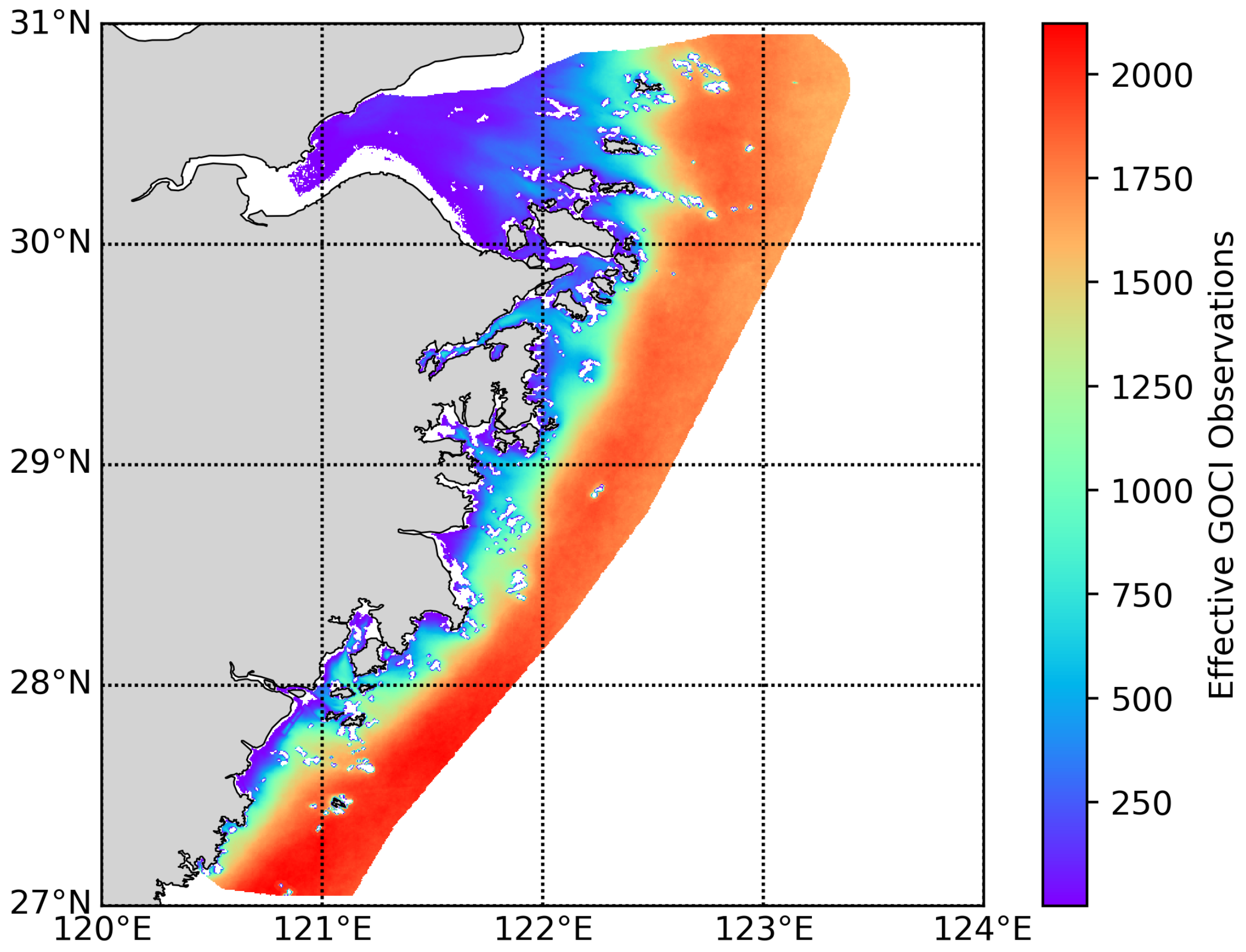
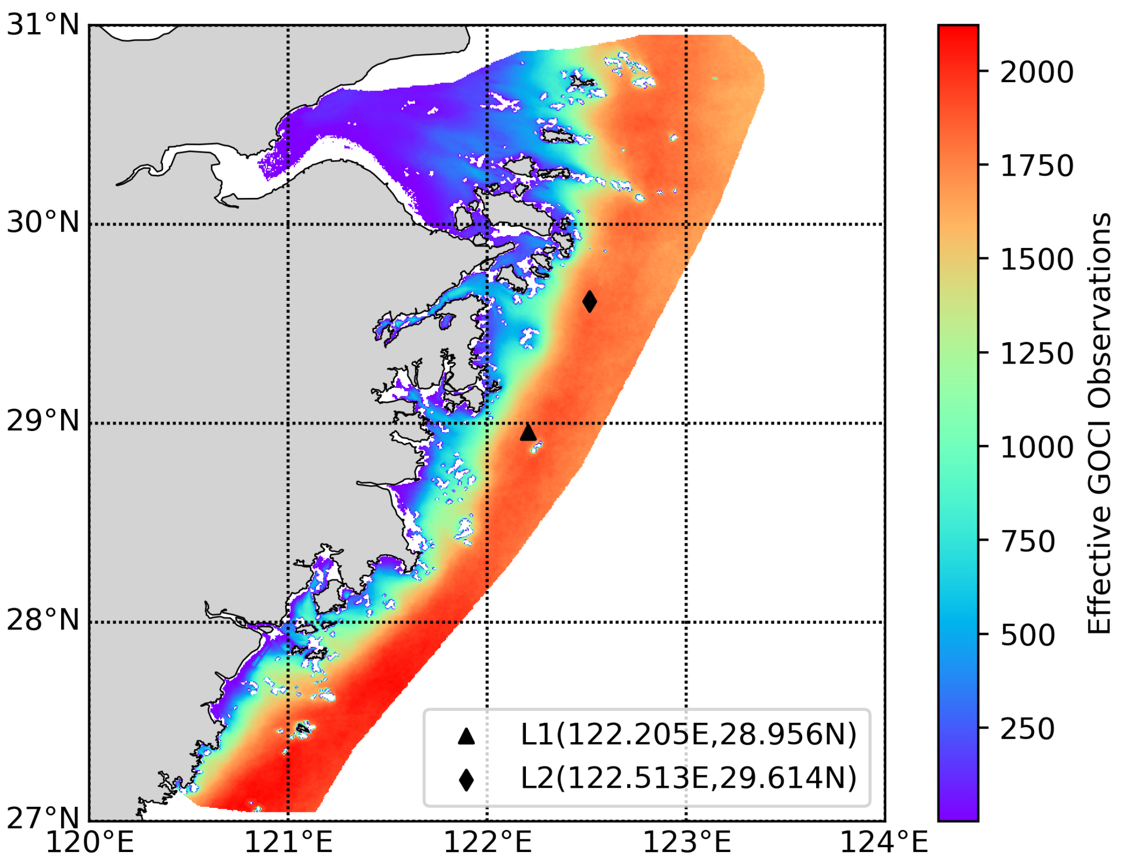
2.1. Study Area

Although HABs are a worldwide problem, they appear particularly severe in China [21], and have been reported in the East China Sea every year in the last decade [22], with the coastal waters of Zhejiang Province suffering the most [23]. From 2014 to 2018, the HAB frequency in the coastal waters of Zhejiang accounted for $41.06\%$ of the total in national waters, and the cumulative area accounted for $36.66\%$ of the national total area [22].

2.2. Long-Term Multisource Satellite Data

As a complex ecological anomaly, HAB results from the combined action of multiple factors. The use of multisource datasets and their analysis with statistical methods is a prerequisite to fully understanding HABs’ onset mechanisms and dynamics [24].

In this study, the data used were divided into two categories: (1) CHL-a, for directly characterizing HABs; and (2) photosynthetically active radiation (PAR) and sea surface temperature (SST) combined to provide a more complete assessment of the underlying factors. As shown in

Table 1. List of the long-term multi-source satellite data.

Parameters	Source	Temporal Range	Temporal Resolution	Spatial Resolution
CHL-a	KOSC GOCI	1 April 2011–31 August 2019	Hourly	500 m
PAR	NASA MODIS		Daily	4 km
G1SST	NOAA Multi-Sensor			1 km
CHL-a	OCCCI Multi-Sensor	6 September 1997–6 September 2017		4 km

, the CHL-a data included the Geostationary Ocean Color Imager (GOCI) 500 m hourly CHL-a from the Korea Ocean Satellite Center (KOSC) and 4 km daily CHL-a from the Ocean Colour Climate Change Initiative (OCCCI), where the KOSC GOCI CHL-a data were retrieved from the remote sensing reflectance data (produced by GDPS 2.0.0 beta version with default settings) by the OC3G algorithm and the OCCCI CHL-a data were daily composites of merged sensor products. The PAR is defined as the quantum energy flux from the Sun in the 400–700 nm range. For ocean color applications, the PAR is a common input for modeling marine primary productivity. The PAR values used in this research were the daily averages of the L3B data from the Moderate Resolution Imaging Spectroradiometer (Modis). The SST data used were the Global 1 km SST (G1SST) data, which combine satellite data from several different sensors and in situ data from drifting and moored buoys, maintaining the fine spatial and temporal resolution needed by SST inputs for a variety of oceanic and atmospheric applications. Considering the launch date of GOCI, the GOCI CHL-a, MODIS PAR, and NOAA G1SST data were unified from 1 April 2011 to 31 August 2019. The OCCCI CHL-a data ranged from 6 September 1997 to 31 August 2019, as the 20-year averaged (climatology) data to fill in missing GOCI CHL-a data.

3. LSTM–EVA-Based Two-Step Detection Scheme

Although GOCI has a higher time resolution as a geostationary satellite and can therefore obtain more effective data than polar orbiting satellites, it is still affected by clouds and aerosols, resulting in a poor data availability rate. As shown in Figure 1, from 1 April 2011 to 31 August 2019, effective GOCI observations of CHL-a in the coastal waters of Zhejiang accounted for up to $22.22\%$ of the total observations, but they dropped to only $11.67\%$ in sea areas close to land. It is extremely difficult to directly perform a spatiotemporal analysis with such incomplete and inexact satellite data.

To address this, an LSTM–EVA-based two-step detection scheme was proposed. In this scheme, LSTMs were trained for each selected coordinate to find potential HAB dates by analyzing the anomalous differences between the predicted and actual values using historical observations. For each potential HAB date, an HAB spatial extraction was then performed based on the selected coordinate using the EVA approach.

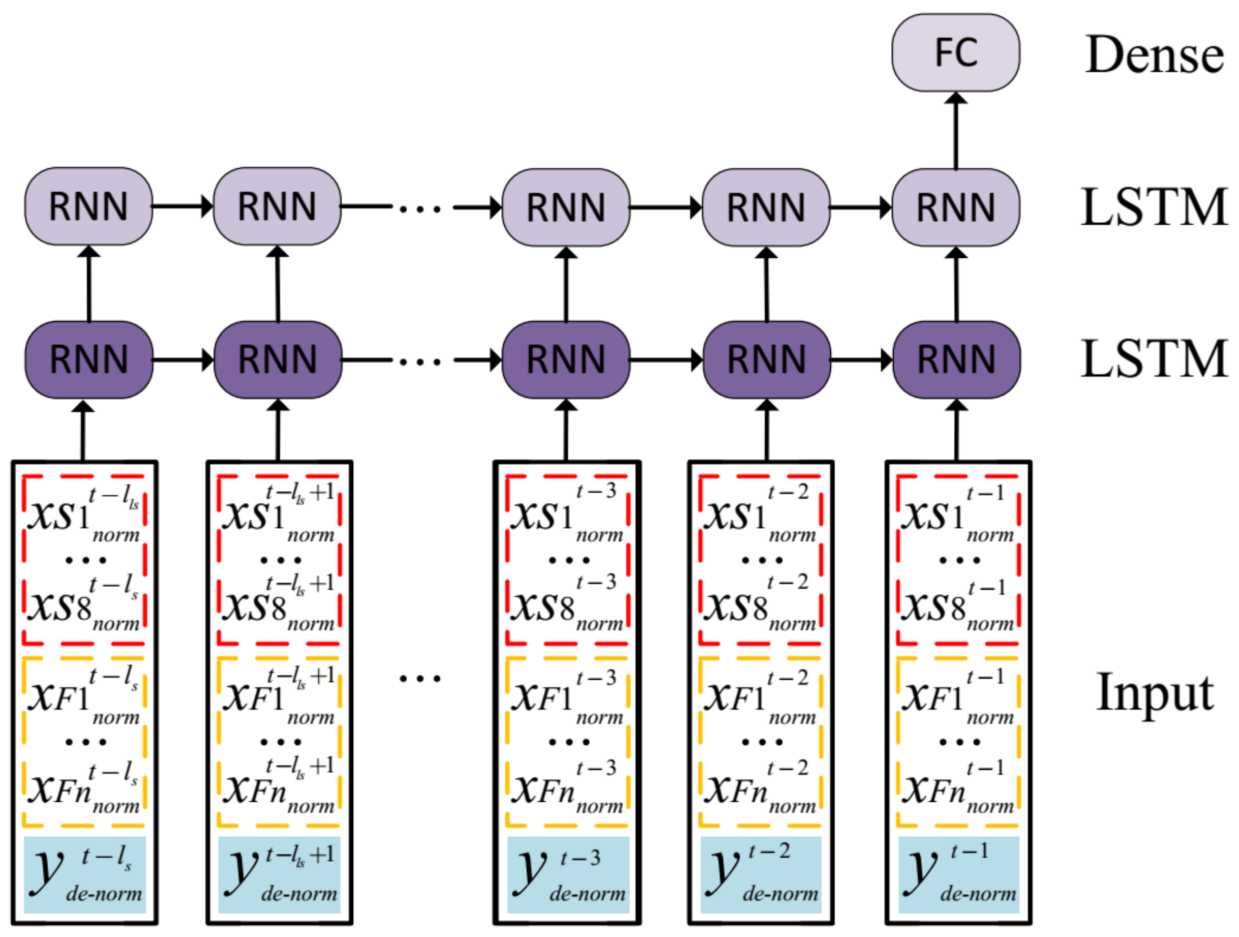
3.1. LSTM-Based Temporal Detection

As a variation of the recurrent neural network (RNN), LSTM represents a significant leap forward for efficiently processing and prioritizing historical information to make accurate predictions. Compared with deep neural networks and early RNNs, LSTM has an improved ability to maintain the memory of long-term dependencies because of the introduction of a weighted self-loop, conditioned on context, that allows it to forget past information in addition to accumulating new information [25,26,27]. The inherent properties of LSTM make it an ideal candidate for anomaly detection tasks involving nonlinear time-series streams of data, driving the increasing use of LSTM networks in this field, with LSTM models fitted on nominal data and the models’ predictions compared with actual data stream values using a set of anomaly detection rules [26,28,29,30,31,32].

In this study, based on LSTM, for the newly observed satellite data at time $t+1$, a sequence of a certain length $l_b$ can be constructed from the historical observations for the selected coordinate, that is, from time $t-l_b+1$ to time t, to predict a value ${\widehat{y}}_{t+1}$ at time $t+1$, and the prediction error $e_{t+1}$ can be expressed as the absolute difference between ${\widehat{y}}_{t+1}$ and the observed value $y_{t+1}$. By sliding the time window one step ahead and using the same pattern, a prediction error series for each day was obtained:

$$E=\{e_{t+1},\dots ,e_{t+l_f+1}\}$$

(1)

where $l_f$ is the length of the prediction error sequence. To then evaluate whether newly observed values are significant, we set a threshold for the prediction errors, and values corresponding to prediction errors above the threshold were classified as anomalies. To determine the threshold, a common method is to make Gaussian assumptions of the error distribution and set the threshold at a fixed multiple of the standard deviation $\sigma \left(E\right)$ from the mean $\mu \left(E\right)$. The probability curve based on the Gaussian distribution has the following characteristics: the value within the range of $\mu \pm \sigma$ covers $68.27\%$ of the data; the value within the range of $\mu \pm 2\sigma$ covers $95.45\%$ of the data; and the value within the value range of $\mu \pm 3\sigma$ covers $99.73\%$ of the data. However, the above probability assumption is only valid when the sample strictly follows the Gaussian distribution. For highly complex ocean systems that change continuously, this method is likely to lead to false positives.

Hundman et al. [33] proposed a complementary unsupervised anomaly thresholding approach to offer false-positive mitigation strategies. The threshold was still set at multiples of $\sigma$ from $\mu$, but the multiple value was determined by the sample. However, their approach was best suited to postprocessing. Inspired by their strategy, we propose an improved approach, where, as in Hundman et al., for the prediction error series E, a new sequence $U=\left\{{\tilde{u}}_k\right\}$ of length k is obtained by

$${\tilde{u}}_k=\mu \left(E\right)+r_k\sigma \left(E\right)$$

(2)

where $r_k$ is a monotonically increasing positive sequence such as $\{1,2,3,\dots \}$, and the sequence U is called the candidate threshold sequence; however, the difference is that, for each element ${\tilde{u}}_k$ in U, the threshold is judged by the following criteria

$$s_k=\frac{\Delta \mu \left(E_k\right)}{\mu \left(E\right)}+\frac{\Delta \sigma \left(E_k\right)}{\sigma \left(E\right)}$$

(3)

where $\Delta \mu \left(E_k\right)=\mu \left(E\right)-\mu \left(\{e_i\in E|e_i<{\tilde{u}}_k\}\right)$ and $\Delta \sigma \left(E_k\right)=\sigma \left(E\right)-\sigma \left(\{e_i\in E|e_i<{\tilde{u}}_k\}\right)$. If $e_{t+l_f+1}$ is an anomalous value, as $r_k$ increases, $\Delta \mu$ and $\Delta \sigma$ will increase more significantly, until when ${\tilde{u}}_k>e_{t+l_f+1}$, $s_k$ is equal to 0 and remains unchanged; if $e_{t+l_f+1}$ is not an anomalous value, $s_k$ will not change significantly with the increase of $r_k$. Therefore, the ${\tilde{u}}_k$ corresponding to the largest $s_k$ is selected as the threshold for determining whether $e_{t+l_f+1}$ is anomalous.

3.2. EVA-Based Spatial Extraction

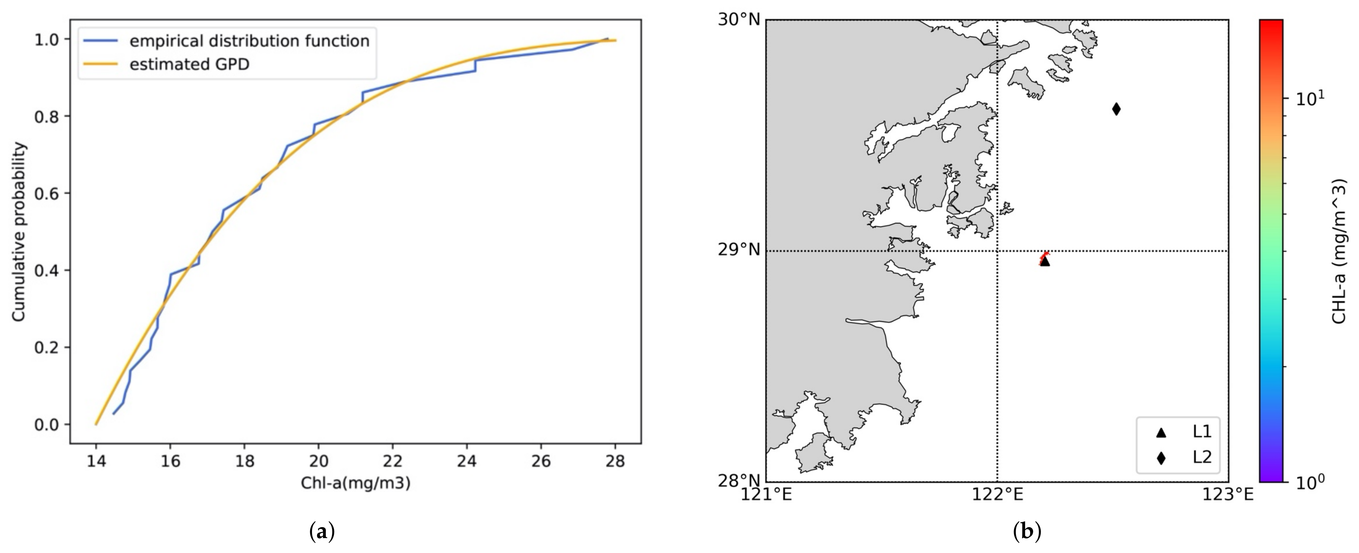
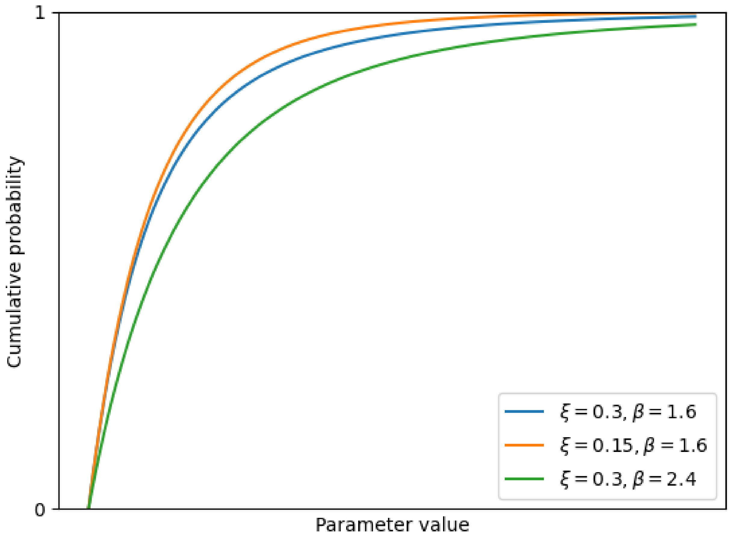
LSTM-based HAB temporal detection cannot reveal the spatial distribution of HABs, and the probability of a pixel-led misjudgment of the incomplete and inexact satellite image is far greater than that of a spatial misjudgment. Therefore, we regarded the abnormal date determined in the previous section as a potential HAB date, and further examined the spatial anomaly distribution. Specifically, we adopted EVA theory to test the fit of HAB areas.

3.2.1. EVA Theory

EVA is a branch of statistics dealing with extreme deviations from the median of probability distributions. This type of research has wide applicability in fields such as climatology, anomaly detection, and financial analysis [34,35,36]. Rather than estimating the cumulative distribution function (CDF) of a variable, the EVA approach estimates directly the CDF of the extreme events that happened for the variable. In this paper, we applied the peaks-over-threshold (POT) method to estimate the distribution of the extreme events. Details about this method can be found in Appendix A or in [37].

It has been proved in [38] that, by applying the POT method, if the threshold u (that determines how extreme the event is) is chosen large enough, the distribution of the extreme events can be approximated by a generalized Pareto distribution (GPD) (see Appendix A for details), $G_{\xi ,\beta }\left(x\right)$, with scale parameter $\beta >0$ and shape parameter $\xi$ defined as follows:

$$G_{\xi ,\beta }\left(x\right)=\left\{\begin{array}{cc}1-{(1+\xi \frac{x}{\beta })}^{-\frac{1}{\xi }},\hfill & if\xi \ne 0\hfill \\ 1-e^{-\frac{x}{\beta }},\hfill & if\xi =0.\hfill \end{array}\right.$$

(4)

However, how to select the threshold u is still an open question. Essentially, u should be chosen to be as large as possible, so the GPD gives a better approximation of the distribution of extreme events. However, if u is too large there will not be enough observations, which could cause overfitting of the GPD function. These factors result in a bias–variance tradeoff for the choice of u.

3.2.2. Dynamic Thresholds

For a selected coordinate, the CHL-a value c at a certain date can be judged by the LSTM-based HAB temporal detection method as a potential abnormality. Considering their spatial correlation, some $\tilde{c}$ adjacent to c can be regarded as the threshold for the extraction of the HAB range (adopting the marching squares algorithm [39]), and $V=\left\{v_i\right|v_i\ge \tilde{c}\}$ provides the CHL-a values of all pixels in this range. A new sequence $C=\left\{{\tilde{c}}_m\right\}$ is obtained by ${\tilde{c}}_m=c\pm 0.25k$, where $k=\{0,1,2,3,\dots \}$, and the sequence C is called the candidate HAB extraction threshold sequence. For each ${\tilde{c}}_m$, a corresponding $V_m$ can be determined. Then, a GPD is estimated based on the observations of $V_m$. Similarly, the optimal threshold $\tilde{c}$ is chosen based on the following unsupervised criteria

$$p_m=\frac{\xi }{\Delta \xi }\frac{\Delta \beta }{\beta }$$

(5)

where $\Delta \xi$ and $\Delta \beta$ denote the difference of the estimate of $\xi$ and $\beta$, respectively, between two threshold candidates ${\tilde{c}}_m$ and ${\tilde{c}}_{m+1}$, and $p_m$ represents the change rate of the CDF.

The threshold determines the starting point of the CDF on the x-axis, and its change should affect the distribution’s tail behavior less. As shown in Figure 2, for the same rate variation, the GPD shape is more sensitive to the value of $\beta$ than to the value of $\xi$. When the candidate threshold is close to the optimal threshold, the shape of the CDF changes the most. In order to maintain the heavy tail behavior, the change rate of $\beta$ is greater than that of $\xi$, and thus maximizes the value of $p_m$, that is, the corresponding ${\tilde{c}}_m$ is the optimal threshold. In particular, when $\Delta \xi =0$, we set $p_m=\frac{\Delta \beta }{\beta }$ because the GPD’s tail behavior is uniquely determined by $\Delta \beta$.

4. Experiment and Discussion

4.1. Representative Sites

The selection of representative sites was based on the following considerations: (1) there were recorded HAB events at the selected sites, and also valid GOCI observation on HAB days, (2) the selected sites needed to have a relatively large number of valid GOCI observations for more a accurate time series analysis, (3) the LSTM model was required to be trained separately on each site, so we used the time series data of 2011 to 2016 for model training, and based on the consideration (1) and (2), representative sites were selected from HAB events during 2017–2018, meanwhile 2019 was used as an HAB unknown reference. We selected two representative sites in Zhejiang coastal waters as our study coordinates for LSTM detection, denoted L1 and L2, as shown in Figure 3. L1 (122.205E, 28.9567N) is located in the Yushan waters of Ningbo, where a large-scale HAB event of up to 420 square kilometers occurred from June to July 2017. L2 (122.5136E, 29.6144N) is located in the sea near Liuheng Island, Zhoushan, where another HAB event of up to 50 square kilometers occurred in May 2017.

4.2. Data Preprocessing

Before feeding the historical observations into LSTM for training, the CHL-a time series of each selected coordinate was preprocessed by spatiotemporal interpolation to obtain a more continuous sequence, and then deseasonalized for more accurate predictions. Combining the proposed LSTM model, historical observations meant the interpolated CHL-a sequence, which were obtained by spatiotemporal interpolation of the GOCI and OCCCI data. Since we were predicting CHL-a, the prediction error could be obtained by subtracting the predicted CHL-a sequence from the historical CHL-a sequence. We assumed that the prediction error followed a Gaussian-like distribution, and any prediction error value that did not fit this distribution was marked as an anomaly, that is, a potential HAB date.

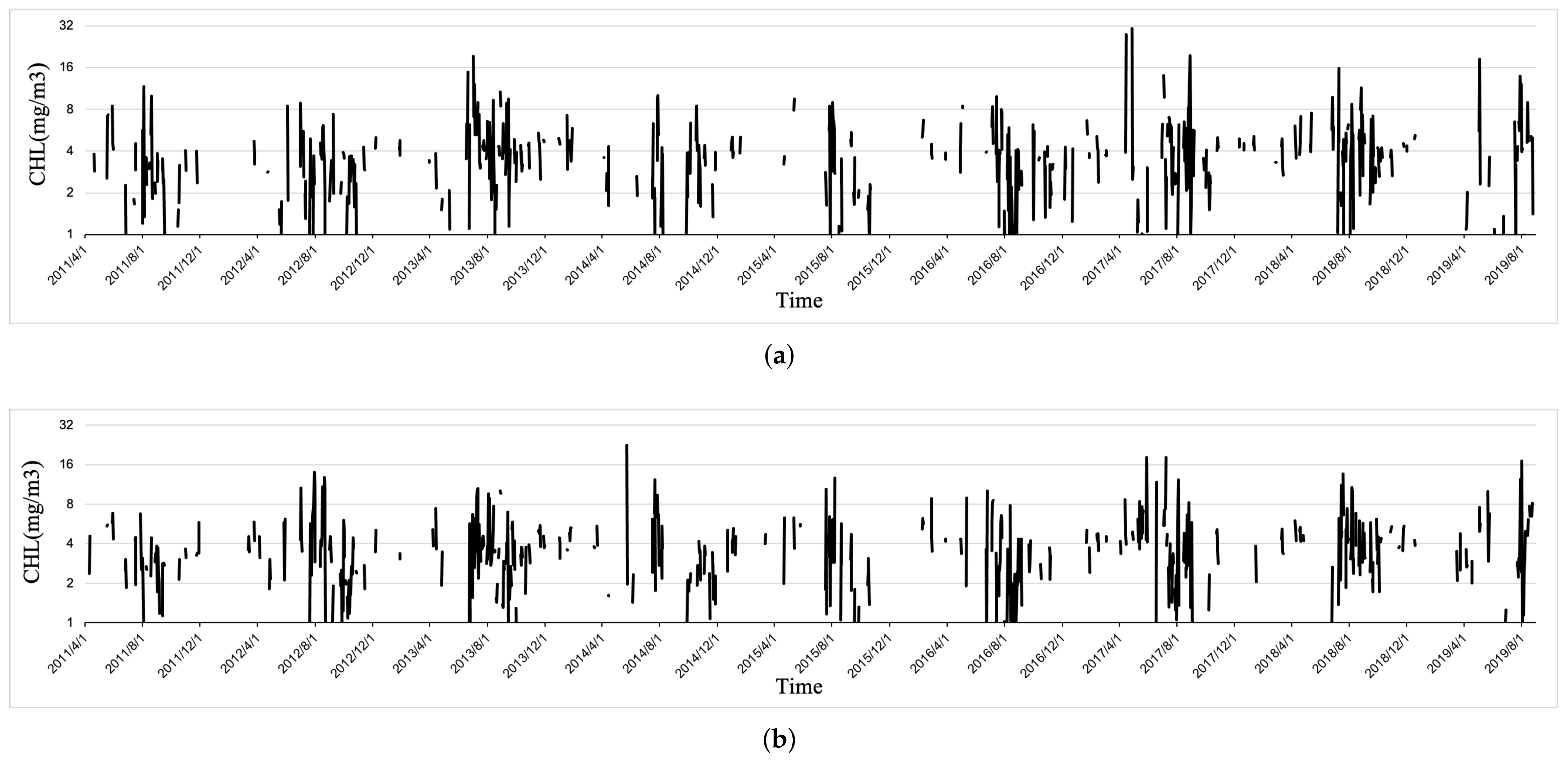
4.2.1. Time Series Extraction

Considering the inconsistent temporal resolution of GOCI CHL-a, MODIS PAR, and NOAA G1SST data and the lower accuracy and quality of ocean color remote sensing under low light conditions [40], we adopted the middle three sets of the eight GOCI observations and averaged them to form a unified temporal resolution. The daily CHL-aat L1 and L2 from 1 April 2011 to 31 August 2019 are shown in Figure 4.

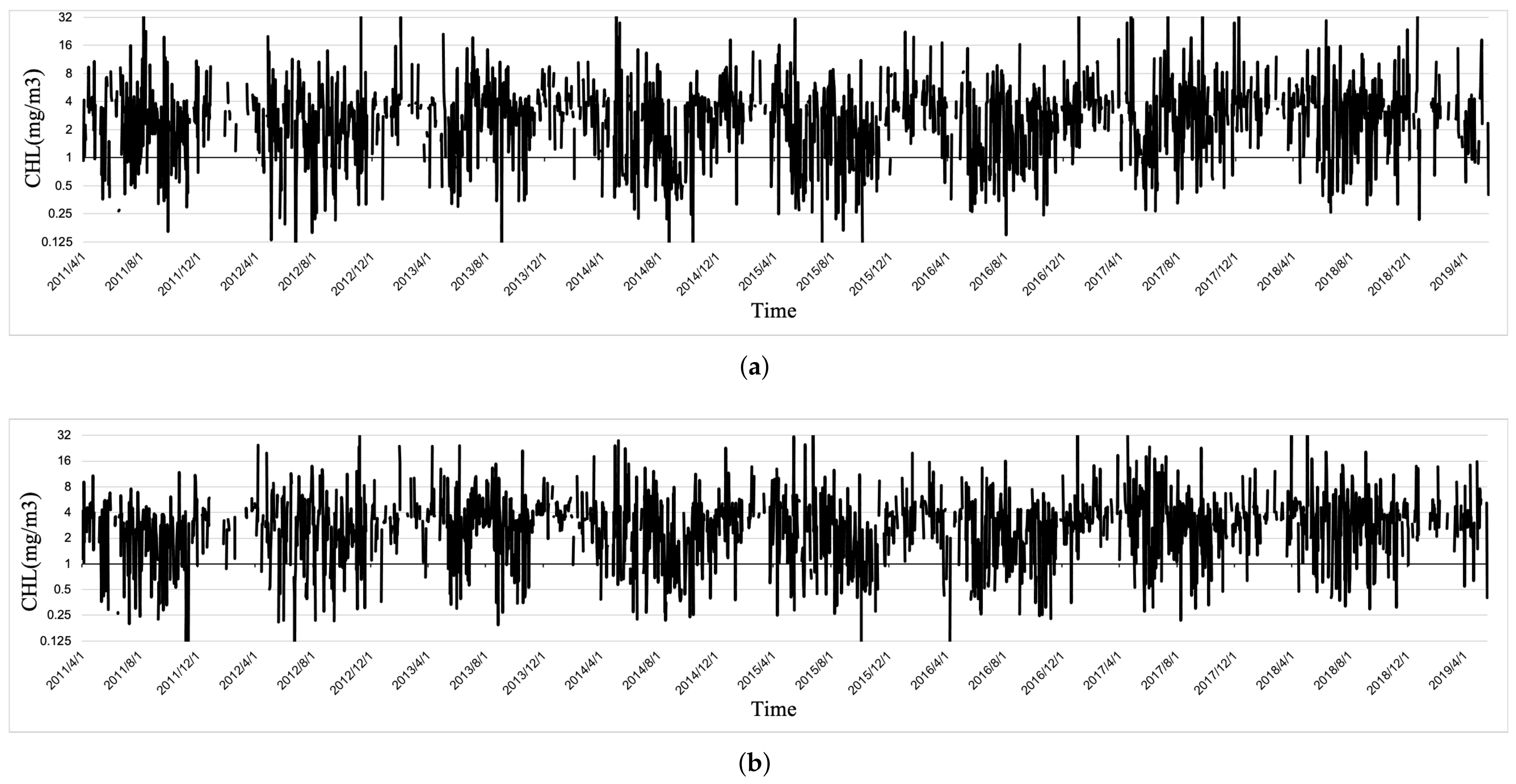
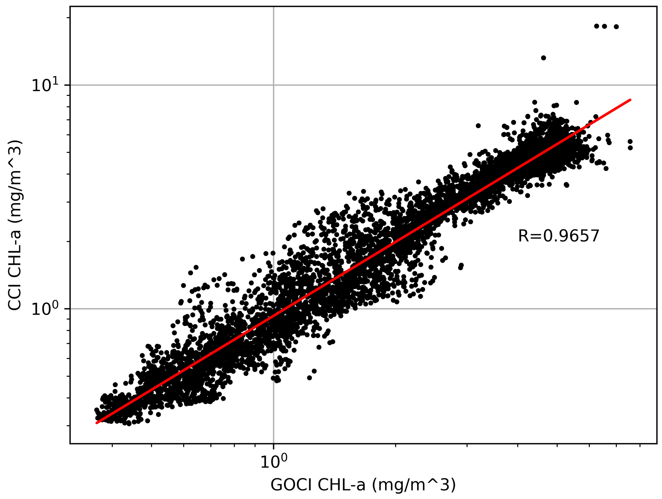
4.2.2. Interpolation of the GOCI CHL-a Time Series

When adopting the LSTM network for predictions, the original GOCI CHL-a time series was divided into multiple subsequences through a sliding window as feature vector inputs; thus, the short-term continuity of the sliding window needed to be guaranteed, otherwise the lack of samples and features would lead to underfitting during predictions. Therefore, the missing GOCI CHL-a time series needed to be interpolated, for which we adopted the following two methods.

First, a spatial interpolation was adopted. Larger spatial sampling windows reduce the credibility of the data, whereas smaller spatial sampling windows may lead to insufficient effective data. Therefore, we adopted a floating distance strategy, gradually increasing the search range from one pixel until a valid pixel value was found, up to a maximum search range.

The interpolated data were not an accurate expression of the target parameters at the original coordinates, so for all pixel values obtained by interpolation there were corresponding spatial weight coefficients used for abnormality discrimination, defined as

$$w=\sqrt[n]{k^d}$$

(6)

where $k\in (0,1)$ is the custom adjustment coefficient, n is the number of effective pixels for sampling, and d is the spatial distance.

Second, we sampled from historical data. The 20-year historical OCCCI CHL-a daily average from 1997 to 2017 accounted for the missing GOCI CHL-a data in the original sequence. To avoid affecting the normal training of the LSTM network by sampling single climatological data multiple times, we randomly distributed the climatological data and sampled them only once.

However, there were inevitable differences between the CHL-a values retrieved by GOCI and OCCCI due to the differences in their sensor performance (e.g., bands and calibration accuracy) and retrieval algorithms (e.g., atmospheric correction and CHL-a algorithms) [41]. To remove these systematic differences, we compared the annual mean CHL-a for each of the pixels derived from GOCI with those derived from OCCCI during their overlapping periods (2011 to 2019), as shown in Figure 5. Thus, we normalized the OCCCI CHL-a by the GOCI CHL-a data according to a linear regression on the logarithmic scale, based on the data in Figure 5 as

$$log\left(\mathit{OCCCI}\right)=1.0901log\left(\mathit{GOCI}\right)-0.0323$$

(7)

and $R=0.9657$ was the correlation coefficient.

Additionally, the as for the spatially interpolated data, a corresponding weight coefficient (fixed at 0) was set for the abnormality discrimination, i.e., values that could not be judged as abnormal. The CHL interpolation sequences at L1 and L2 obtained according to the above method are shown in Figure 6.

4.2.3. Deseasonalization

Deseasonalization, also known as seasonal adjustment, helps to explore the true trend of the time series. In previous studies, when there was seasonality in the time series, forecasts from neural networks estimated on deseasonalized data were significantly more accurate than those based on unadjusted data [42]. To deseasonalize the CHL-a time series, we modeled the seasonality by a combination of sine and cosine [43] as

$$S\left(t\right)=\sum _{n=1}^N(a_{n}cos\left(\frac{2\pi nt}{P}\right)+b_{n}sin\left(\frac{2\pi nt}{P}\right))$$

(8)

whose parameters can be expressed as a column vector

$$\beta ={(a_1,b_1,\dots ,a_N,b_N)}^{\top }$$

(9)

where we have

$$S\left(t\right)=Y\left(t\right)\beta$$

(10)

The initialization of $\beta$ was represented as $\beta$∼$\mathit{Normal}(0,{\sigma }^2)$ and the seasonal effect was controlled by the value of $\sigma$, with larger values representing more obvious seasonal effects.

4.2.4. Model Input and Parameters

To fully consider the spatiotemporal correlation of the original image, we also fed the CHL-a values from around L1 and L2 as spatial features, together with PAR and G1SST series, into the LSTM network, and output the CHL-a prediction sequence. The network parameters are listed in

Table 2. Model Parameters.

Description	Value
Hidden layers	2
Units in hidden layers	36,12
Sequence length	35
Prediction length	7
Dropout	0.3
Optimizer	Adam

. Specifically, the model only had two hidden layers, where the first hidden layer had 36 units and the second had 12 units. We set the time window of the input sequence to 35 to provide a balance between performance and training times. The prediction length was set to 7, with the assumption that forcing the model to predict further into the future would encourage better predictions in the short term (one step ahead in this case) because the loss would be calculated for all seven predictions and be used for training. Combining the above factors, the neural network design is shown as Figure 7.

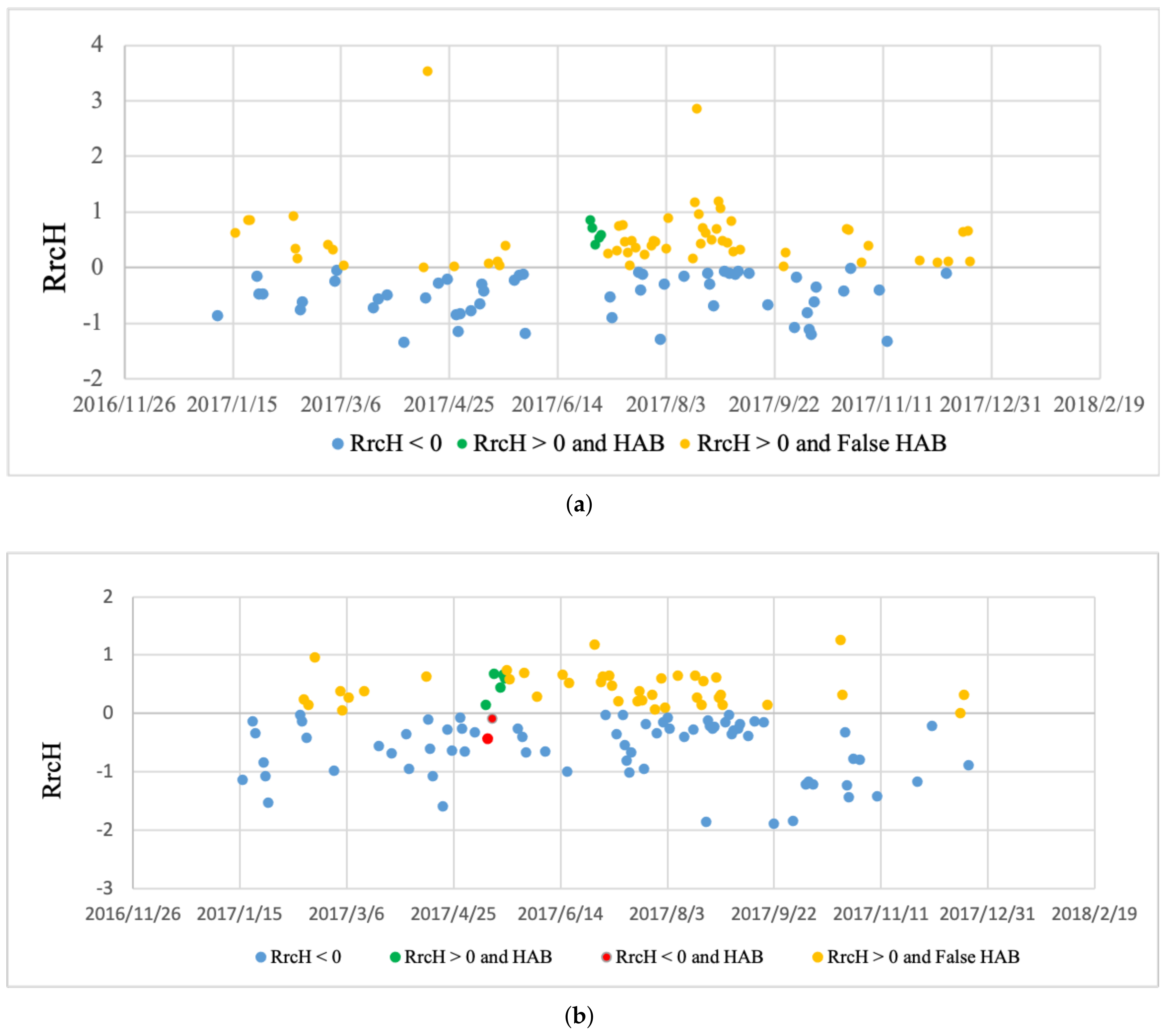
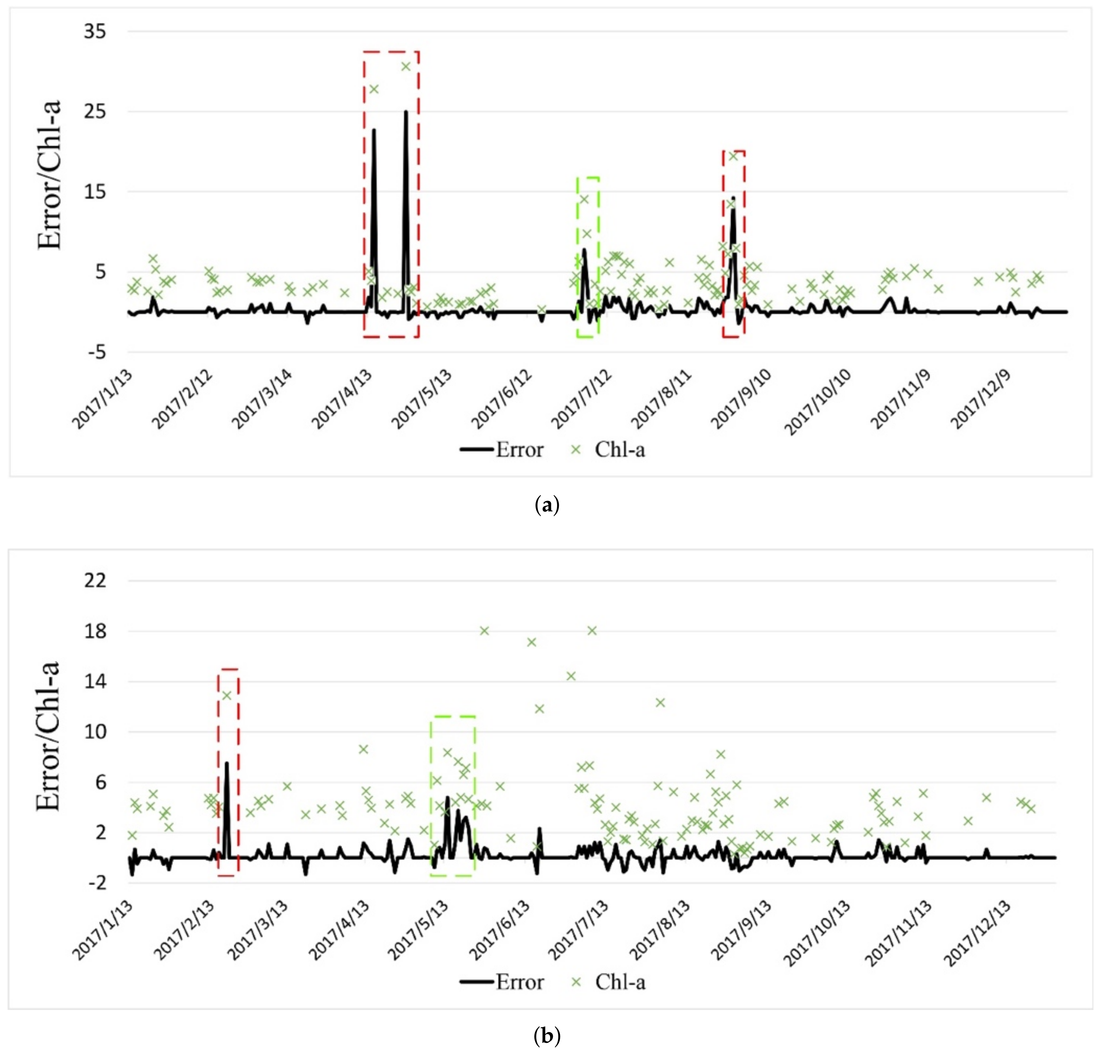
4.3. HAB Temporal Detection Results and Discussion

Once the predictions were generated, a time window of 30 days was set to determine whether these predictions represented potential HAB dates by comparing the prediction errors using the method detailed in Section 3.1. Furthermore, the potential HAB dates detected at L1 and L2 in 2017 are shown in Figure 8. We employed $MAE=\frac{1}{m}{\sum }_{t=1}^m|\widehat{y_t}-y_t|$ to evaluate the quantitative accuracy of the LSTM prediction and we obtained the result that $MA{E}_{L1}=0.1462$, $MA{E}_{L2}=0.1363$ (after normalization). Since the sequence had undergone the interpolation and deseasonalization preprocessing, the results of Figure 8 are the prediction errors of the actual values, which have been multiplied by their corresponding interpolation weight coefficients.

Specifically, a large-scale HAB occurred near L1 from 16 June to 6 July 2017, and another large-scale HAB occurred near L2 from 10 to 19 May 2017. Among the effective remote sensing observation days, 3 and 4 July 2017 at L1, and 14 and 18 May 2017 at L2 were determined as potential HAB dates.

However, as shown by the red dashed line, L1 on 15 and 27 April 2017, and L2 on 19 February 2017 were all identified as potential HAB dates, but no HABs were recorded on those days. Valid remote sensing data also existed on 29 June, 30 June, and 1 July 2017 at L1, with relatively low CHL-a values of 4.45 mg/m${}^3$, 4.64 mg/m${}^3$ and 4.93 mg/m${}^3$, respectively, but these were not identified as potential HAB dates.

The above potentially correct identifications and misjudgments all required a further analysis through the EVA-based HAB spatial extraction method. However, first we compared our results with a traditional spectral-characteristics-based HAB detection approach to illustrate the importance and advancement of our two-step detection scheme. Specifically, we used the HAB extraction index RrcH proposed by [44], defined as:

$$\begin{array}{cc}\hfill \mathrm{RrcH}=& (Rrc\left(555\right)-Rrc\left(443\right))\left(\frac{490-443}{555-443}\right)\hfill \\ \hfill & +Rrc\left(443\right)-Rrc\left(490\right)\hfill \end{array}$$

(11)

where Rrc is the Rayleigh-corrected reflectance.

They found that the RrcH index identified significant differences between different types of water. For instance, turbid water bodies had values lower than 0; clean water had both positive and negative values, fluctuating around 0; and HABs had values higher than 0. We thereby constructed the RrcH scatter plots at L1 and L2 for 2017, as shown in Figure 9 (the RrcH indices are expanded by 1000 times).

Compared with the LSTM-based HAB temporal detection method, the RrcH index produced more misjudgments, mainly identifying HAB occurrences when none were recorded. Therefore, if the RrcH index alone were used for the HAB detection, then a large number of false alarms could be generated. However, if some coordinates were selected in advance for the HAB temporal detection, the false alarm rate could be greatly reduced, as proved by the effectiveness of the LSTM-based HAB temporal detection method in experiments at L1 and L2.

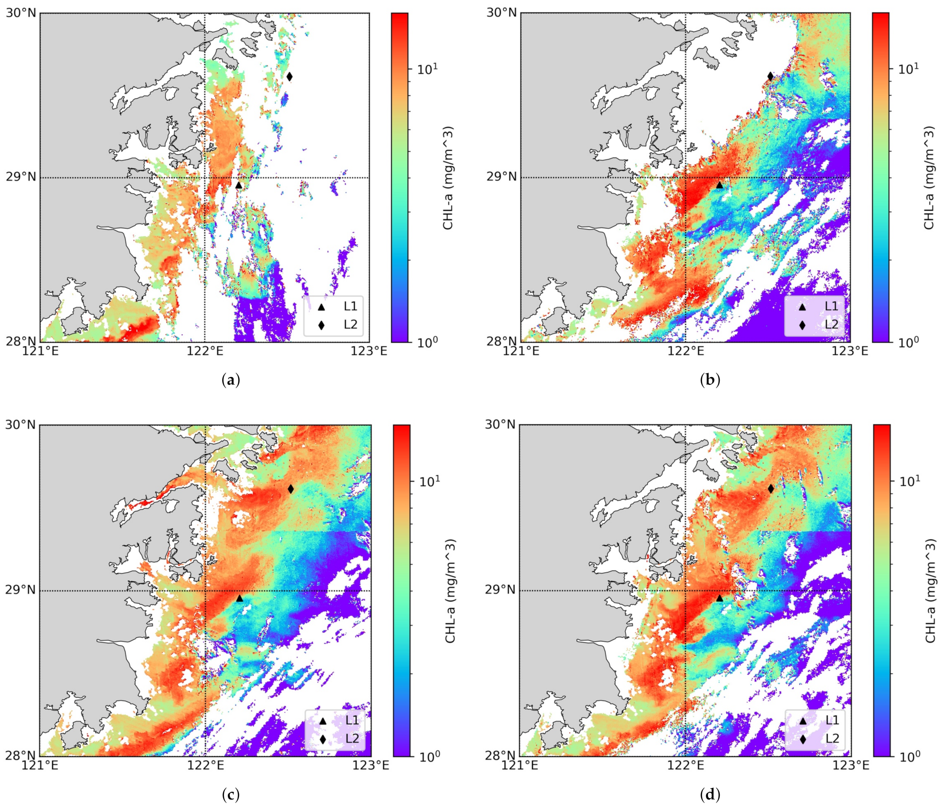
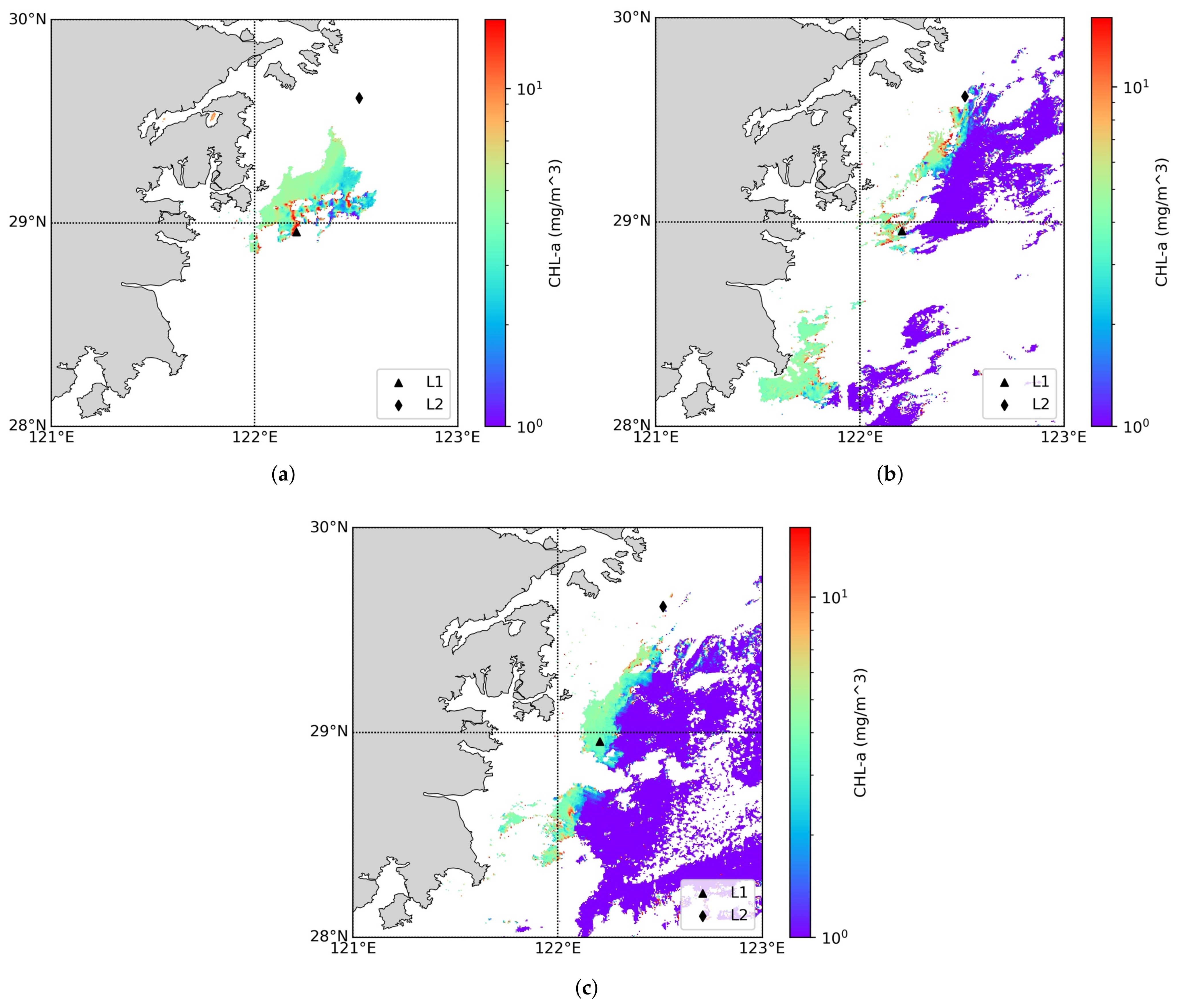
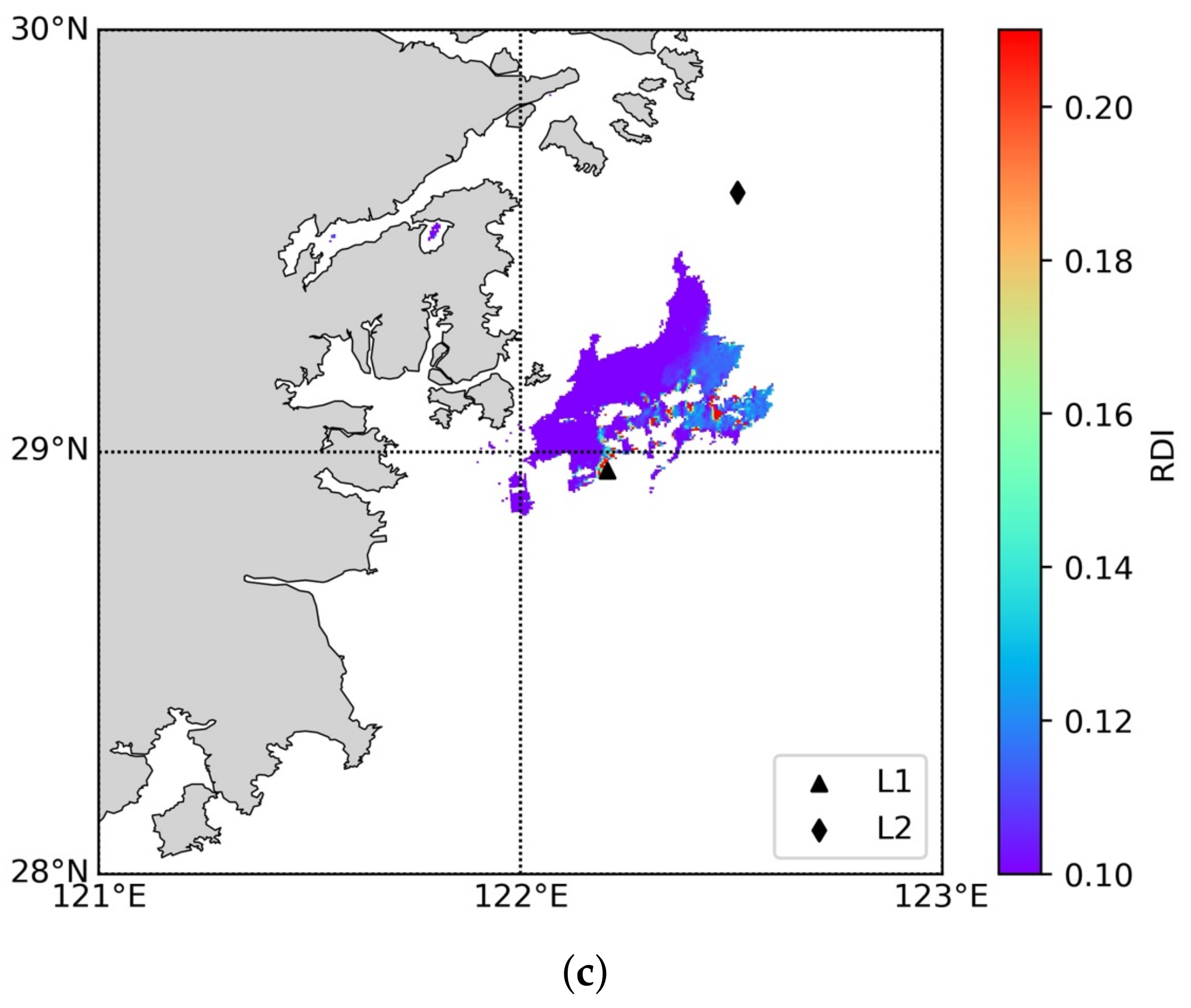
4.4. HAB Spatial Extraction Results and Discussion

In this section, we analyzed the three cases at L1 in the previous section in which recorded HABs were correctly identified as potential HAB dates, unrecorded HABs were identified as potential HAB dates, and recorded HABs were not identified as potential HAB dates. Specifically, based on the coordinates of selected sites and potential HAB dates, the EVA model could be further used to examine the spatial distribution of HABs. That is, according to the coordinate and a certain CHL-a threshold, a certain range was screened, and all CHL-a values in this range were considered to follow a GPD distribution. Notably, when we unified the time resolution of GOCI with the other remote sensing data, we used a daily average of GOCI data, but in practical applications the hourly GOCI data provide critical additional ability to understand the short-term HAB dynamics in highly dynamic environments. Therefore, the following EVA-based HAB spatial extraction was performed on the hourly GOCI data.

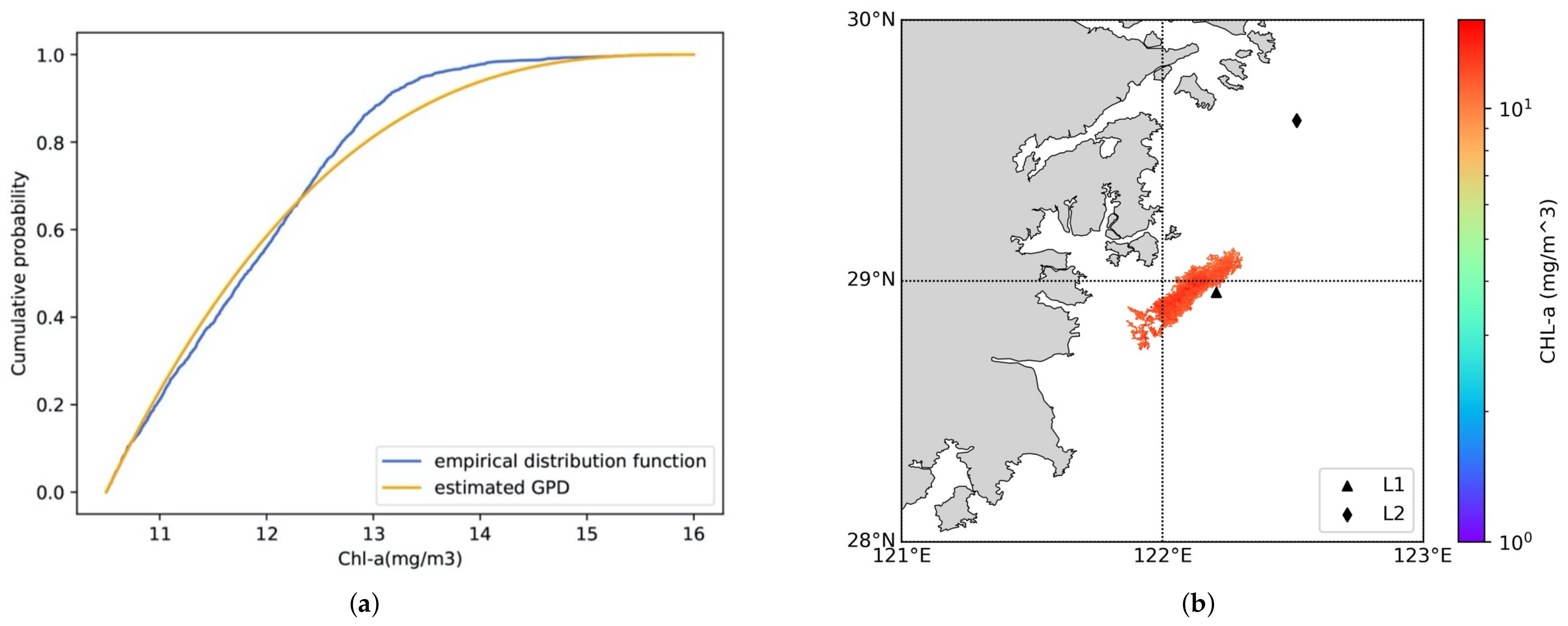
4.4.1. Recorded HAB Correctly Identified as Potential HAB Date

First, we considered the scenario in which recorded HABs were correctly identified as potential HAB dates. As previously mentioned, potential HAB dates at L1 were identified as 3 and 4 July 2017. The GOCI CHL-a images at 12:00 on these days are shown in Figure 10a,b. The effective data coverage of the CHL-a near L1 on 4 July was higher than on 3 July, so for this section, we analyzed 4 July 2017 as an example.

The GOCI CHL-a at 10:00 and 11:00 on 4 July 2017 are shown in Figure 10c,d. Then, the CHL-a values at L1 at 10:00, 11:00, and 12:00 on 4 July were used as the initial thresholds to approach the optimal thresholds, and the EVA-based HAB spatial extraction method was used to analyze the respective HAB spatial distributions. The threshold criteria identified at different thresholds for these three times are shown in

Table 3. GPD fitting results at different thresholds at 10:00 on 4 July 2017.

Thresholds	8.00	8.25	8.50	8.75	9.00	9.25	9.50	9.75
$p_m$	1.6826	0	2.2630	0	2.2776	0	0	1.6782
Thresholds	10.00	10.25	10.50	10.75	11.00	11.25	11.50
$p_m$	2.4888	0	2.7136	2.4728	1.7894	1.5337	1.7710

,

Table 4. GPD fitting results under different thresholds at 11:00 on 4 July 2017.

Thresholds	10.50	10.75	11.00	11.25	11.50	11.75	12.00	12.25	12.50	12.75
$p_m$	0	1.9275	1.9948	1.5791	1.6360	1.8384	1.9096	1.5605	1.9004	1.5200
Thresholds	13.00	13.25	13.50	13.75	14.00	14.25	14.50	14.75	15.00
$p_m$	1.8892	1.4713	2.6471	1.7540	0	0.7941	0.3407	0	0.0550

and

Table 5. GPD fitting results under different thresholds at 12:00 on 4 July 2017.

Thresholds	10.75	11.00	11.25	11.50	11.75	12.00	12.25	12.50	12.75
$p_m$	1.5126	2.1054	1.5384	2.1111	2.0556	2.1176	2.0588	2.1250	1.9250
Thresholds	13.00	13.25	13.50	13.75	14.00	14.25	14.50	14.75
$p_m$	2.1239	2.2038	1.9898	0.4226	0.3581	0.1899	0.1114	0.0461

, the optimal threshold is marked in bold.

Referring to the above results, we set the HAB extraction thresholds near L1 of the three images from 10:00 to 12:00 on 4 July 2017, as 10.5 mg/m${}^3$, 13.5 mg/m${}^3$, and 13.25 mg/m${}^3$, respectively. The GPD fit results and the HAB spatial ranges extracted at these thresholds are shown in Figure 11.

Overall, the CDF of the HAB area extracted by the selected threshold at these three times was close to the GPD, although the fitting result at 10:00 on 4 July 2017 was inferior to the latter two. Furthermore, the HAB spatial range extracted by the above method was compared with the Red tide Detection Index (RDI) distributions proposed by [9], defined as:

$$RDI=(\frac{1}{Rrc\left(660\right)}-\frac{1}{Rrc\left(555\right)})Rrc\left(745\right)$$

(12)

Furthermore, the RDI results are shown in Figure 12. The HAB spatial range extracted by our EVA-based method was similar to the high RDI range, giving our method some credibility.

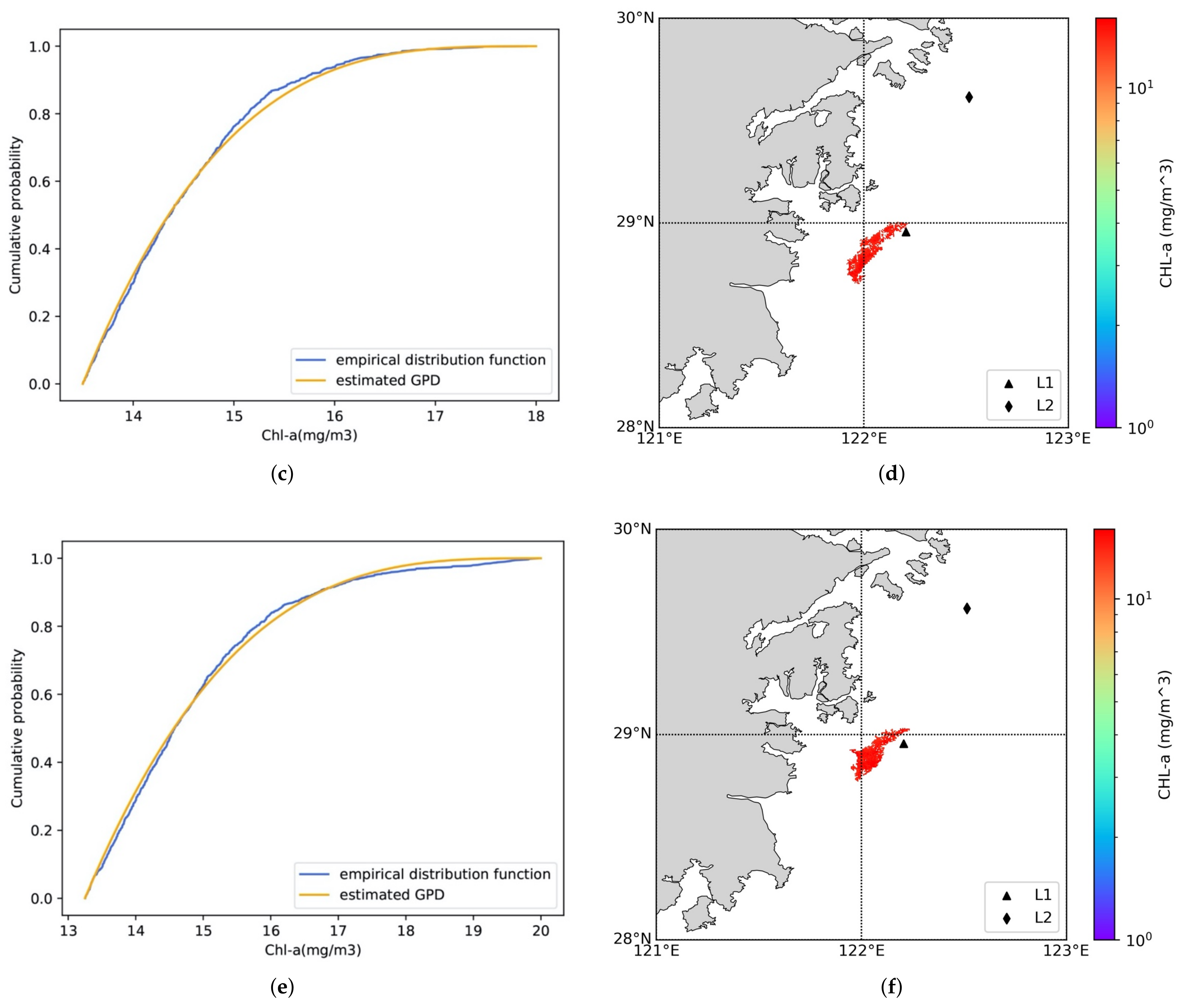
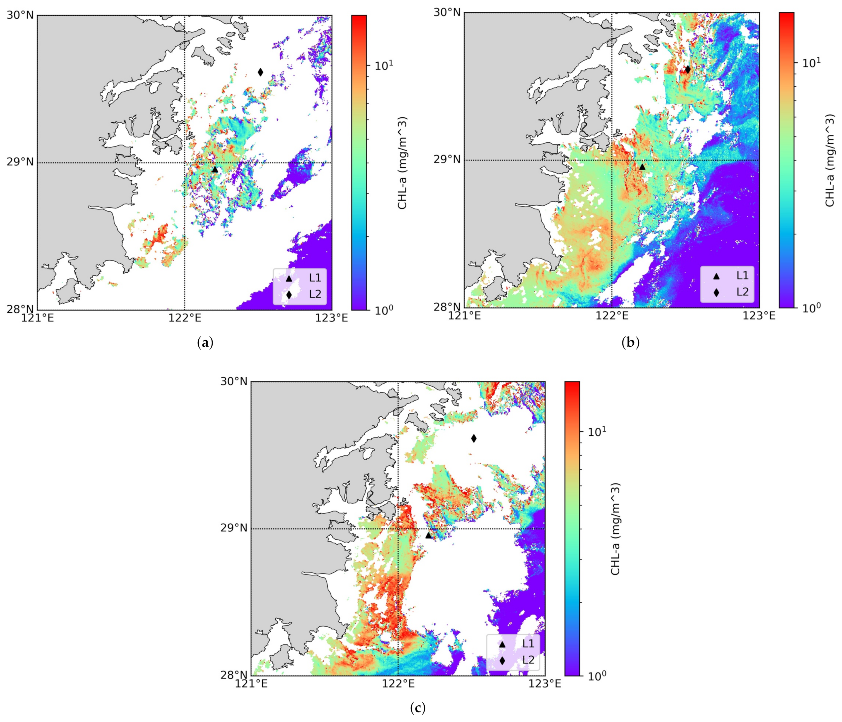
4.4.2. Unrecorded HAB Identified as Potential HAB Date

Second, we considered the scenario in which unrecorded HABs were identified as potential HAB dates. As previously mentioned, potential HAB dates at L1 were identified as 15 and 27 April 2017, but there were no records of HABs on these two days. The GOCI CHL-a images with valid data on these days are shown in Figure 13.

From these images, the anomaly at L1 on 27 April was identified at 11:00. Clearly, this was a single point anomaly that could be eliminated by the marching squares algorithm. By comparison, the anomaly at L1 on 15 April came from the value at 10:00, which affected a wider area, so only this potential anomaly was analyzed.

Adopting the same process as in the previous subsection, the results were as follows: in

Table 6. GPD fitting results under different thresholds at 10:00 on 15 April 2017.

Thresholds	8.00	8.25	8.50	8.75	9.00	9.25	9.50	9.75	10.00
$p_m$	4.5000	6.0000	6.6667	6.3333	4.6667	5.8000	6.0000	5.4000	3.6667
Thresholds	10.25	10.50	10.75	11.00	11.25	11.50	11.75	12.00	12.25
$p_m$	4.3846	6.0000	5.0000	4.2500	5.8000	5.4000	4.3750	2.0000	5.4444
Thresholds	12.50	12.75	13.00	13.25	13.50	13.75	14.00	14.25	14.50
$p_m$	6.3333	4.8889	4.2500	5.8571	3.8333	14.0000	6.8889	4.4000	4.1000

, the number in bold represents the initial threshold at L1 at 10:00 on 15 April set at 27.79 mg/m${}^3$, and the GPD fit result for the CHL-a HAB and RID distributions are shown in Figure 14.

As shown in Figure 14, the CDF of the HAB area extracted by the selected optimal threshold at 10:00 on 15 April 2017 was close to the GPD. The CDF was not as smooth as those at the three times of day on 4 July 2017 because of its smaller sample size (36 samples), but this did not affect the determination of the optimal threshold. The HAB spatial range extracted by our proposed EVA-based approach was similar to the results of the RDI index analysis. Therefore, there may have been an unrecorded HAB on 15 April 2017, detected by the potential abnormality identified by our method. The unrecorded reason may be that the HAB area was so small (about 9 km${}^2$) that it was not detected.

4.4.3. Recorded HAB Not Identified as Potential HAB Date

Third, we considered the scenario in which recorded HABs were not identified as potential HAB dates. As previously mentioned, our method did not identify the recorded HABs on 29 June, 30 June, and 1 July, 2017 at L1 as potential HAB dates. The valid observed GOCI CHL-a images on these days are shown in Figure 15.

Although there were valid observations at L1 on these three days, the CHL-a values were generally low, which was the main reason they were not identified as potential HAB dates. We assumed that the coordinates of L1 were the positions where the HAB was originally discovered and reported. However, considering that HABs move with ocean currents, there were no HABs to observe at L1 on these three days.

5. Conclusions

In this paper, a two-step scheme combining LSTM with EVA for HAB detection was designed to handle incomplete and inexact marine remote sensing data. The LSTM network built a normal time series model for a selected coordinate by long-term multisource satellite data. This model detected potential HAB dates by utilizing the LSTM predictive error for an approximated Gaussian distribution. For each potential HAB date, the EVA approach then extracted the HAB distribution from the selected coordinate with consideration of the spatial correlations. The case study in Zhejiang coastal waters showed that our method combined the advantages of both LSTM and EVA models. It not only exploited LSTM’s good prediction performance, well learned with long-term multisource historical satellite information to reduce the false alarm rate, but also achieved a dynamic HAB extraction through the EVA fitting.

However, this proposed approach has some shortcomings that will require improvement. First, the prediction model constructed by PAR and SST was insufficiently comprehensive to fully demonstrate the causes of HABs. This was mainly limited by the existing data coverage and acquisition capabilities. However, as detection hardware and data processing technology mature, a more complete ocean dynamics model could be considered. Second, the case study was only verified for two coordinates with corresponding HAB records, which could not fully demonstrate the accuracy of the LSTM–EVA model. As more data are accumulated and HABs are recorded, a more comprehensive verification could be performed. Third, for the necessity of the LSTM–EVA model, there was no strong coupling relationship between LSTM and EVA, and only a sequential method was proposed for the high quantity of missing GOCI data. If the spatiotemporal data are complete, it is more appropriate to use ConvLSTM or multivariate EVA for direct spatiotemporal modeling.

References

1. Fleming, L.E.; McDonough, N.; Austen, M.; Mee, L.; Moore, M.; Hess, P.; Depledge, M.H.; White, M.; Philippart, K.; Bradbrook, P.; et al. Oceans and human health: A rising tide of challenges and opportunities for Europe. Mar. Environ. Res. 2014, 99, 16–19. [Google Scholar] [CrossRef] [PubMed]
2. Anderson, D.M. Approaches to monitoring, control and management of harmful algal blooms (HABs). Ocean Coast. Manag. 2009, 52, 342–347. [Google Scholar] [CrossRef] [PubMed]
3. Siswanto, E.; Ishizaka, J.; Tripathy, S.C.; Miyamura, K. Detection of harmful algal blooms of Karenia mikimotoi using MODIS measurements: A case study of Seto-Inland Sea, Japan. Remote Sens. Environ. 2013, 129, 185–196. [Google Scholar] [CrossRef]
4. Stumpf, R.; Culver, M.; Tester, P.; Tomlinson, M.; Kirkpatrick, G.; Pederson, B.; Truby, E.; Ransibrahmanakul, V.; Soracco, M. Monitoring Karenia brevis blooms in the Gulf of Mexico using satellite ocean color imagery and other data. Harmful Algae 2003, 2, 147–160. [Google Scholar] [CrossRef]
5. Tomlinson, M.; Wynne, T.; Stumpf, R. An evaluation of remote sensing techniques for enhanced detection of the toxic dinoflagellate, Karenia brevis. Remote Sens. Environ. 2009, 113, 598–609. [Google Scholar] [CrossRef]
6. Hu, C.; Carder, K.L.; Muller-Karger, F.E. Atmospheric correction of SeaWiFS imagery over turbid coastal waters: A practical method. Remote Sens. Environ. 2000, 74, 195–206. [Google Scholar] [CrossRef]
7. Siegel, D.A.; Wang, M.; Maritorena, S.; Robinson, W. Atmospheric correction of satellite ocean color imagery: The black pixel assumption. Appl. Opt. 2000, 39, 3582–3591. [Google Scholar] [CrossRef]
8. Tao, B.; Mao, Z.; Lei, H.; Pan, D.; Shen, Y.; Bai, Y.; Zhu, Q.; Li, Z. A novel method for discriminating Prorocentrum donghaiense from diatom blooms in the East China Sea using MODIS measurements. Remote Sens. Environ. 2015, 158, 267–280. [Google Scholar] [CrossRef]
9. Shen, F.; Tang, R.; Sun, X.; Liu, D. Simple methods for satellite identification of algal blooms and species using 10-year time series data from the East China Sea. Remote Sens. Environ. 2019, 235, 111484. [Google Scholar] [CrossRef]
10. Ahn, Y.H.; Shanmugam, P. Detecting the red tide algal blooms from satellite ocean color observations in optically complex Northeast-Asia Coastal waters. Remote Sens. Environ. 2006, 103, 419–437. [Google Scholar] [CrossRef]
11. Hu, C.; Muller-Karger, F.E.; Taylor, C.J.; Carder, K.L.; Kelble, C.; Johns, E.; Heil, C.A. Red tide detection and tracing using MODIS fluorescence data: A regional example in SW Florida coastal waters. Remote Sens. Environ. 2005, 97, 311–321. [Google Scholar] [CrossRef]
12. Tester, P.A.; Steidinger, K.A. Gymnodinium breve red tide blooms: Initiation, transport, and consequences of surface circulation. Limnol. Oceanogr. 1997, 42, 1039–1051. [Google Scholar] [CrossRef]
13. Neely, M.B.; Bartels, E.; Cannizzaro, J.; Carder, K.L.; Coble, P.; English, D.; Heil, C.; Hu, C.; Hunt, J.; Ivey, J.; et al. Florida’s Black Water Event. 2004. Available online: https://dspace.mote.org/handle/2075/3022 (accessed on 23 July 2020).
14. Hu, C.; Luerssen, R.; Muller-Karger, F.E.; Carder, K.L.; Heil, C.A. On the remote monitoring of Karenia brevis blooms of the west Florida shelf. Cont. Shelf Res. 2008, 28, 159–176. [Google Scholar] [CrossRef]
15. Gokaraju, B.; Durbha, S.S.; King, R.L.; Younan, N.H. A machine learning based spatio-temporal data mining approach for detection of harmful algal blooms in the Gulf of Mexico. IEEE J. Sel. Top. Appl. Earth Obs. Remote Sens. 2011, 4, 710–720. [Google Scholar] [CrossRef]
16. Gokaraju, B.; Durbha, S.S.; King, R.L.; Younan, N.H. Ensemble methodology using multistage learning for improved detection of harmful algal blooms. IEEE Geosci. Remote Sens. Lett. 2012, 9, 827–831. [Google Scholar] [CrossRef]
17. Hill, P.R.; Kumar, A.; Temimi, M.; Bull, D.R. HABNet: Machine learning, remote sensing-based detection of harmful algal blooms. IEEE J. Sel. Top. Appl. Earth Obs. Remote Sens. 2020, 13, 3229–3239. [Google Scholar] [CrossRef]
18. Liu, W.; Pyrcz, M.J. A spatial correlation-based anomaly detection method for subsurface modeling. Math. Geosci. 2021, 53, 809–822. [Google Scholar] [CrossRef]
19. Hochreiter, S.; Schmidhuber, J. Long short-term memory. Neural Comput. 1997, 9, 1735–1780. [Google Scholar] [CrossRef]
20. Fisher, R.A.; Tippett, L.H.C. Limiting forms of the frequency distribution of the largest or smallest member of a sample. In Mathematical Proceedings of the Cambridge Philosophical Society; Cambridge University Press: Cambridge, UK, 1928; Volume 24, pp. 180–190. [Google Scholar]
21. Li, X.; Shang, S.; Lee, Z.; Lin, G.; Zhang, Y.; Wu, J.; Kang, Z.; Liu, X.; Yin, C.; Gao, Y. Detection and Biomass Estimation of Phaeocystis globosa Blooms off Southern China From UAV-Based Hyperspectral Measurements. IEEE Trans. Geosci. Remote Sens. 2021, 60, 4200513. [Google Scholar] [CrossRef]
22. Ministry of Natural Resources. Available online: https://www.mnr.gov.cn/sj/sjfw/hy/gbgg/zghyzhgb/ (accessed on 23 July 2022).
23. Lou, X.; Hu, C. Diurnal changes of a harmful algal bloom in the East China Sea: Observations from GOCI. Remote Sens. Environ. 2014, 140, 562–572. [Google Scholar] [CrossRef]
24. Blondeau-Patissier, D.; Gower, J.F.; Dekker, A.G.; Phinn, S.R.; Brando, V.E. A review of ocean color remote sensing methods and statistical techniques for the detection, mapping and analysis of phytoplankton blooms in coastal and open oceans. Prog. Oceanogr. 2014, 123, 123–144. [Google Scholar] [CrossRef]
25. Sak, H.; Senior, A.W.; Beaufays, F. Long short-term memory recurrent neural network architectures for large scale acoustic modeling. In Proceedings of the 15th Annual Conference of the International Speech Communication Association, Singapore, 14–18 September 2014. [Google Scholar]
26. Malhotra, P.; Vig, L.; Shroff, G.; Agarwal, P. Long short term memory networks for anomaly detection in time series. In Proceedings of the 23rd European Symposium on Artificial Neural Networks, Computational Intelligence and Machine Learning, ESANN 2015, Bruges, Belgium, 22–24 April 2015. [Google Scholar]
27. Goodfellow, I.; Bengio, Y.; Courville, A. Deep Learning; MIT Press: Cambridge, MA, USA, 2016. [Google Scholar]
28. Chauhan, S.; Vig, L. Anomaly detection in ECG time signals via deep long short-term memory networks. In Proceedings of the 2015 IEEE International Conference on Data Science and Advanced Analytics (DSAA), Paris, France, 19–21 October 2015; pp. 1–7. [Google Scholar]
29. Bontemps, L.; Cao, V.L.; McDermott, J.; Le-Khac, N.A. Collective anomaly detection based on long short-term memory recurrent neural networks. In Proceedings of the International Conference on Future Data and Security Engineering, Can Tho City, Vietnam, 23–25 November 2016; pp. 141–152. [Google Scholar]
30. Malhotra, P.; Ramakrishnan, A.; Anand, G.; Vig, L.; Agarwal, P.; Shroff, G. LSTM-based encoder-decoder for multi-sensor anomaly detection. arXiv 2016, arXiv:1607.00148. [Google Scholar]
31. Nanduri, A.; Sherry, L. Anomaly detection in aircraft data using Recurrent Neural Networks (RNN). In Proceedings of the 2016 Integrated Communications Navigation and Surveillance (ICNS), Herndon, VA, USA, 19–21 April 2016; p. 5C2-1. [Google Scholar]
32. Padrón-Hidalgo, J.A.; Laparra, V.; Camps-Valls, G. Unsupervised Anomaly and Change Detection With Multivariate Gaussianization. IEEE Trans. Geosci. Remote Sens. 2021, 60, 5513010. [Google Scholar] [CrossRef]
33. Hundman, K.; Constantinou, V.; Laporte, C.; Colwell, I.; Soderstrom, T. Detecting spacecraft anomalies using lstms and nonparametric dynamic thresholding. In Proceedings of the 24th ACM SIGKDD International Conference on Knowledge Discovery & Data Mining, London, UK, 19–23 August 2018; pp. 387–395. [Google Scholar]
34. Smith, R.L. Extreme value analysis of environmental time series: An application to trend detection in ground-level ozone. Stat. Sci. 1989, 4, 367–377. [Google Scholar]
35. Roberts, S.J. Novelty detection using extreme value statistics. IEE Proc.-Vision Image Signal Process. 1999, 146, 124–129. [Google Scholar] [CrossRef]
36. Embrechts, P.; Klüppelberg, C.; Mikosch, T. Modelling Extremal Events: For Insurance and Finance; Springer Science & Business Media: Berlin/Heidelberg, Germany, 2013; Volume 33. [Google Scholar]
37. McNeil, A.; Embrechts, P.; Frey, R. Quantitative Risk Management: Concepts, Techniques and Tools; Princeton Series in Finance; New Age International: New Delhi, India, 2010. [Google Scholar]
38. Pickands, J., III. Statistical inference using extreme order statistics. Ann. Stat. 1975, 3, 119–131. [Google Scholar]
39. Maple, C. Geometric design and space planning using the marching squares and marching cube algorithms. In Proceedings of the 2003 International Conference on Geometric Modeling and Graphics, London, UK, 16–18 July 2003; pp. 90–95. [Google Scholar]
40. Choi, J.K.; Park, Y.J.; Lee, B.R.; Eom, J.; Moon, J.E.; Ryu, J.H. Application of the Geostationary Ocean Color Imager (GOCI) to mapping the temporal dynamics of coastal water turbidity. Remote Sens. Environ. 2014, 146, 24–35. [Google Scholar] [CrossRef]
41. Morel, A.; Huot, Y.; Gentili, B.; Werdell, P.J.; Hooker, S.B.; Franz, B.A. Examining the consistency of products derived from various ocean color sensors in open ocean (Case 1) waters in the perspective of a multi-sensor approach. Remote Sens. Environ. 2007, 111, 69–88. [Google Scholar] [CrossRef]
42. Nelson, M.; Hill, T.; Remus, W.; O’Connor, M. Time series forecasting using neural networks: Should the data be deseasonalized first? J. Forecast. 1999, 18, 359–367. [Google Scholar] [CrossRef]
43. Taylor, S.J.; Letham, B. Forecasting at scale. Am. Stat. 2018, 72, 37–45. [Google Scholar] [CrossRef]
44. Feng, Z.; Xuying, Y.; Xiaoxiao, S.; Zhenhong, D.; Renyi, L. Developing Process Detection of Red Tide Based on Multi-Temporal GOCI Images. In Proceedings of the 2018 10th IAPR Workshop on Pattern Recognition in Remote Sensing (PRRS), Beijing, China, 19–20 August 2018; pp. 1–6. [Google Scholar]
45. Balkema, A.A.; De Haan, L. Residual life time at great age. Ann. Probab. 1974, 2, 792–804. [Google Scholar] [CrossRef]
Figure 1. Effective GOCI observations of CHL-a in the coastal waters of Zhejiang from 1 April 2011 to 31 August 2019.
Remotesensing 14 03918 g001
Figure 2. Shapes of GPDs under different values of ξ and β .
Remotesensing 14 03918 g002
Figure 3. Representative sites.
Remotesensing 14 03918 g003
Figure 4. Original CHL-a time series at (a) L1 and (b) L2.
Remotesensing 14 03918 g004
Figure 5. Comparison of annual mean OCCCI CHL-a and GOCI CHL-a from 2011 to 2019. The red line is the linear regression on the logarithmic scale.
Remotesensing 14 03918 g005
Figure 6. Interpolated CHL-a time series at (a) L1 and (b) L2.
Remotesensing 14 03918 g006
Figure 7. Architecture of the proposed LSTM neural network model for CHL-a prediction. X S i are the spatial features, X F i are the underlying factors features (PAT and SST in this paper), and y de norm is the deseasonalized CHL-a.
Remotesensing 14 03918 g007
Figure 8. Prediction error and CHL-a values at (a) L1 and (b) L2 during 2017. The black broken line represents the prediction error, the green scattered dots represent the actual CHL-a value, the red dashed line represents potential HAB dates misjudgments, and the green dashed line represents potential HAB dates’ correct identification according to the HAB records.
Remotesensing 14 03918 g008
Figure 9. RrcH scatter plot at (a) L1 and (b) L2 during 2017. The green and blue points are correctly identified points, which, respectively, represent HAB occurrences with RrcH > 0 and no recorded HABs with RrcH < 0. The yellow and red points are misjudged points, which, respectively, represent no recorded HABs with RrcH > 0 and HAB occurrences with RrcH < 0.
Remotesensing 14 03918 g009
Figure 10. CHL-a at (a) 12:00 on 3 July, (b) 12:00 on 4 July, (c) 10:00 on 4 July, and (d) 11:00 on 4 July, in 2017.
Remotesensing 14 03918 g010
Figure 11. GPD fit results and HAB spatial distribution at L1 at (a,b) 10:00 with 10.5 mg/m 3 , (c,d) 11:00 with 13.5 mg/m 3 , and (e,f) 12:00 with 13.25 mg/m 3 as the extraction threshold, on 4 July 2017.
Remotesensing 14 03918 g011aRemotesensing 14 03918 g011b
Figure 12. RDI at (a) 10:00, (b) 11:00, and (c) 12:00, on 4 July in 2017.
Remotesensing 14 03918 g012
Figure 13. CHL-a at (a) 10:00 on 15 April, (b) 11:00 on 27 April, and (c) 12:00 on 27 April, in 2017.
Remotesensing 14 03918 g013
Figure 14. Results at L1 at 10:00 on 15 April 2017. (a,b) GPD fits and HAB spatial distribution with 13.75 mg/m 3 as the extraction threshold, (c) RDI result.
Remotesensing 14 03918 g014aRemotesensing 14 03918 g014b
Figure 15. CHL-a at (a) 11:00 on 29 June, (b) 11:00 on 30 June, and (c) 11:00 on 1 July, in 2017.
Remotesensing 14 03918 g015