Estimating Global Anthropogenic CO₂ Gridded Emissions Using a Data-Driven Stacked Random Forest Regression Model

Abstract

The accurate estimation of anthropogenic carbon emissions is of great significance for understanding the global carbon cycle and guides the setting and implementation of global climate policy and CO₂ emission-reduction goals. This study built a data-driven stacked random forest regression model for estimating gridded global fossil fuel CO₂ emissions. The driving variables include the annual features of column-averaged CO₂ dry-air mole fraction (XCO₂) anomalies based on their ecofloristic zone, night-time light data from the Visible Infrared Imaging Radiometer Suite (VIIRS), terrestrial carbon fluxes, and vegetation parameters. A two-layer stacked random forest regression model was built to fit 1° gridded inventory of open-source data inventory for anthropogenic CO₂ (ODIAC). Then, the model was trained using the 2014–2018 dataset to estimate emissions in 2019, which provided a higher accuracy compared with a single-layer model with an R² of 0.766 and an RMSE of 0.359. The predicted gridded emissions are consistent with Global Carbon Grid at 1° scale with an R² of 0.665, and the national total emissions provided a higher R² at 0.977 with the Global Carbon Project (GCP) data, as compared to the ODIAC (R² = 0.956) data, in European countries. This study demonstrates that data-driven random forest regression models are capable of estimating anthropogenic CO₂ emissions at a grid scale.

1. Introduction

The increase in greenhouse gases (GHG) in the atmosphere is the main cause of global climate change, and the increase in anthropogenic CO₂ emissions has become the main cause of a 48% surge in atmospheric CO₂ concentrations [1,2]. Half of these anthropogenic CO₂ emissions have occurred in the past 50 years for fossil fuel combustion [3]. The reduction in GHG emissions is regarded as the most effective way to curb global warming [4]. The accurate estimation of anthropogenic CO₂ emissions is the basis for setting and implementing global emission reductions goals and has an influence on national policy actions [5,6]. In addition, it can provide a deeper understanding in many aspects such as the global carbon cycle, atmospheric chemical transport, and feature climate predictions [7,8].

The approaches to carbon emission estimation have been divided into two types: top-down and bottom-up. The bottom-up approach is widely used to estimate CO₂ emissions, which calculates the emissions from energy consumption and emission factors. Limited by the lack of robustness and timeliness in energy statistics from different countries, especially in less-developed regions, the global bottom-up CO₂ emission inventories can be significantly delayed [9] and the biases cannot be ignored [10,11,12]. The top-down approach combined atmospheric observations with atmospheric transport models [13] to gauge the uncertainty in emission inventories and improve the accuracy of CO₂ emission estimations [14,15,16], but it also faces great challenges in distinguishing anthropogenic CO₂ emissions from natural sources, which results in considerable uncertainty [17]. The space-borne atmosphere CO₂ observations have been widely used to monitor and quantify CO₂ emissions [18,19]. The Greenhouse Gases Observing Satellite (GOSAT), the Orbiting Carbon Observatory-2 (OCO-2), OCO-3, TanSat, and other satellites have provided global XCO₂ data by detecting the short-wavelength infrared reflected from surface and the thermal infrared emitted from surface and atmosphere [20,21,22,23]. Numerous studies have shown that spaceborne XCO₂ data can reflect atmospheric CO₂ concentration changes caused by anthropogenic emissions and provide a way to quantitatively assess the accuracy of these inventories [14,15,24,25,26,27,28]. The spatiotemporal-intensive observation of the OCO-3 satellite has quantified intra-urban variations in XCO₂, which revealed 6 ppm enhancement of XCO₂ compared to the surrounding background in Los Angeles [27]. Both GOSAT and OCO-2 satellite XCO₂ data have reflected the decline in atmospheric CO₂ concentration before and after COVID-19, but the declining value of OCO-2 is larger [28]. The GOSAT identifies consistencies between the model simulations from inventory and the XCO₂ enhancements estimated from observations in North America (ratio is 1.05  ±  0.38, p < 0.1), but it has poor consistency in East Asia (ratio is 1.22  ±  0.32, p < 0.32) [14]. The two approaches are complementary to each other and it is necessary to introduce the satellite observation data into CO₂ emission estimates.

The data-driven machine learning approaches provide a new way to estimate CO₂ emissions. This approach can combine CO₂ emission inventories with various data, especially observational data effectively and avoid uncertainties in the simulation of the carbon cycle as it is insensitive to noise and gaps in the model input parameters [29,30,31]. A series of statistical data such as Gross Domestic Product (GDP), economic growth, population, vehicle mileage, power production, and so on are often selected as the driving data for estimation of CO₂ emissions [32,33,34]. Lei et al. [32] and Kenneth et al. [33] estimate CO₂ emissions in a time series and consider the redundancy of input variables. Yang et al. [35] and Mustafa et al. [36] estimated CO₂ emissions at a regional grid level and the XCO₂ anomalies and the effect of vegetation were considered in their model. The selection of input variables has great significance on the accuracy of anthropogenic CO₂ emission estimates [37,38,39]. It is a feasible way to select input variables according to the process of CO₂ emissions and carbon cycle, which has not been fully investigated at present. This study provides an alternative approach to anthropogenic carbon emission estimation using a data-driven stacked random forest regression model to estimate fossil fuel CO₂ emissions. First, we selected 13 annual features as the driving variables from multi-source data including the following: XCO₂ anomalies to express the atmospheric CO₂ changes; the night-time light to reflect human activities; and the ecosystem respiration (RECO) to directly express the contribution of terrestrial ecosystems on variation in atmospheric XCO₂ and vegetation parameters solar-induced chlorophyll fluorescence (SIF) and enhanced vegetation index (EVI) to indirectly reflect the carbon sequestration ability of vegetation. Then, we designed a two-layer stacking structure with the individual random forest regression models as elements to resolve the significantly uneven distribution of fossil fuel CO₂ emissions. Finally, this stacked random forest regression model was trained using an open-source data inventory for anthropogenic CO₂ (ODIAC) data in 2014–2018 and tested using the data in 2019, and the results were verified and compared to Global Carbon Project (GCP) data. This study demonstrates that a data-driven random forest regression model has the potential to accurately estimate fossil fuel CO₂ emissions at a grid scale.

2. Data and Preprocessing

2.1. Anthropogenic Emission Data

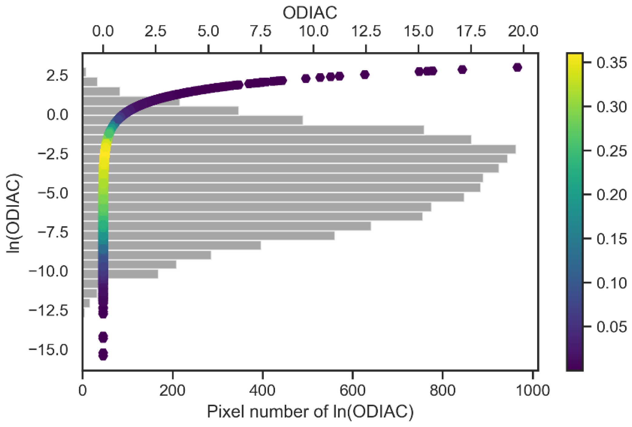
This study involved three anthropogenic emission datasets which were ODIAC, Global Carbon Grid, and GCP results. The ODIAC data was used to train the model and for validation on the test set. The Global Carbon Grid and GCP results were used to compare with our emission estimates at grid scale and national scale, respectively.

2.1.1. ODIAC Data

The ODIAC is a global gridded CO₂ emission inventory of fossil fuel combustion that has been approved and widely used in comparison with other inventories [40,41,42], verification of satellite observations of XCO₂ [43,44], the global carbon cycle [45], and other related research. ODIAC is based on the emission data from the Carbon Dioxide Information Analysis Center (CDIAC) and uses multiple spatial emission proxies to distribute CO₂ emissions on a grid of 1 km × 1 km and 1° × 1° [46]. In this study, we used the natural logarithm form of the annual mean of 1° ODIAC products in 2014–2018 when training the model and restored the model prediction in 2019 to the final emission estimates by exponential transformation [47]. The pixel with ODIAC emissions equaling 0 was directly assigned as the minimum value. Since intense anthropogenic emissions may only cause minor anomalies in atmospheric CO₂ content, which is similar to exponential transformation [24], the logarithmic transformation was used to fit the relationship between the two. At the same time, the values of ODIAC are concentrated near 0, and the logarithmic transformation can expand the value range and makes the sample distribution more dispersed (Figure 1), which enhance discriminations between samples.

2.1.2. Global Carbon Grid Data

The Global Carbon Grid from Global Energy Infrastructure Emissions Database (GID) is a high-resolution gridded inventory of global anthropogenic CO₂ emission which establishes a framework to integrate point sources, country-level sectoral activities and emissions, and transport emissions and distributions [48,49]. The Global Carbon Grid v1.0 provides global CO₂ emission maps with a spatial resolution of 0.1° in 2019 which has been used in research related to gridding of CO₂ emissions [50]. To validate our gridded CO₂ emissions at grid scale, we resampled Global Carbon Grid data to 1° grid by pixel aggregation.

2.1.3. GCP Data

The annually published Global Carbon Budget is a report by the researchers of GCP. The data supplement to the Global Carbon Budget includes the national emissions of most countries and regions in the world. We used the national CO₂ emission data in 2019 from the latest release [51] which added emissions from lime production in China [2] to verify our emission estimates at the national scale.

2.2. Multisource Driving Data

2.2.1. Mapping XCO₂ Anomalies Based on Ecofloristic Zones

The anomalies caused by anthropogenic emissions can be identified by satellite observations of XCO₂ [15,24,25,26,27,28,52]. In this study, we used an XCO₂ space–time expansion product, which is based on the XCO₂ retrievals from GOSAT and OCO-2 satellites [53]. The product completely covers a space ranging from 56°S to 65°N and from 169°W to 180°E with a time resolution of 3 days. The variation in XCO₂ concentration is complex, and it varies based on its ecofloristic zone [54]. Therefore, to enhance the information generated by anthropogenic emissions while distinguishing differences in ecofloristic zones, referring to the method of calculating XCO₂ anomalies proposed by Hakkarainen et al. [24], this study calculated XCO₂ anomalies by ecofloristic zone: each ecofloristic zone was regarded as having the same XCO₂ background value that equaled the median of the area, and the annual mean value of XCO₂ anomalies was used in the model. This study adopted the global ecofloristic zones of the United Nations Food and Agricultural Organization (FAO) and the world is divided into 21 ecological types [55]. The XCO₂ anomalies distinguished by ecofloristic zone (dXCO₂) are derived as:

$${\mathrm{dXCO}}_2={{\mathrm{XCO}}_2}_{\mathrm{original}}-{{\mathrm{XCO}}_2}_{\mathrm{median}}$$

(1)

where ${{\mathrm{XCO}}_2}_{\mathrm{original}}$ represents the original XCO₂ value of each pixel and ${{\mathrm{XCO}}_2}_{\mathrm{median}}$ represents the median of all pixels in the same ecofloristic zone.

2.2.2. Other Driving Data

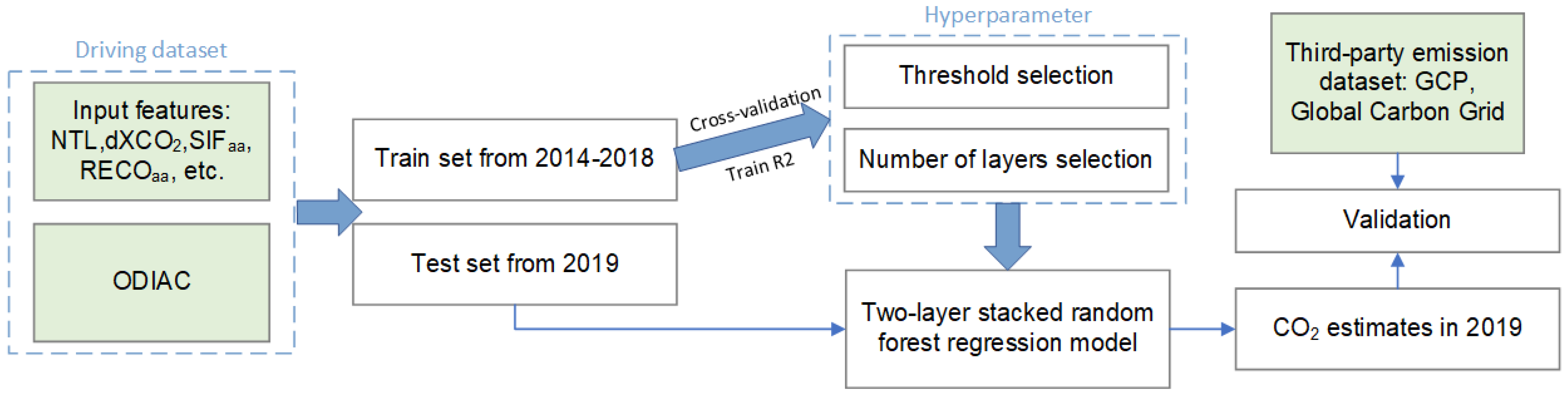
To obtain more information related to anthropogenic CO₂ emission, besides the dXCO₂ mentioned above, the night-time light, terrestrial carbon fluxes parameter, and vegetation parameters were also included in the driving dataset.

The night-time light data was sourced from Visible Infrared Imaging Radiometer Suite (VIIRS) day/night band (DNB) stray light characterization and correction product [56]. Compared with the earlier night-time light dataset, VIIRS DNB has higher spatial and radiation resolutions, it has a stronger detection ability for weak ground radiation signals [57] and this corrected production removes the haze and striping and reduces the offset caused by stray light [56]. The terrestrial carbon fluxes parameter was from RECO data product produced by Zeng et al. [58] with a spatial resolution of 0.1° and a temporal resolution of 10 days. This product is a data-driven upscale product based on FLUXNET 2015 observations by random forest and ranging from 60°S to 80°N, which covers almost all the human activity territory. The vegetation parameters included EVI and SIF. The EVI data was from MOD13C2 v006, which is a monthly product with a spatial resolution of 0.05° and the SIF data was from global ‘OCO-2’ SIF data set (GOSIF) product produced by Li et al. [59] with a spatial resolution of 0.05° and time resolution of 8 days. The two products are both of good temporal and spatial continuity.

3. Methods

A data-driven stacked random forest regression approach was employed to estimate fossil fuel CO₂ emissions. The ODIAC data was used as the fossil fuel CO₂ emissions dataset to train the model and the driving data included 13 annual metrics from XCO₂, night-time light, RECO, SIF, and EVI. All the driving datasets were resized to a resolution of 1° × 1°grids from 2014 to 2019. The two-layer stacked random forest regression model was trained on samples from 2014 to 2018 and tested using samples from 2019 (Figure 2). The uncertainties of model estimates were represented by the standard deviations calculated from the estimates of terminal nodes in 100 trees in the second-layer model [60].

3.1. Variable Selection in the Data-Driven Model

The data-driven model can combine the inventory data and multisource remote sensing data effectively to estimate fossil fuel CO₂ emissions without an accurate simulation of the complicated process. We selected 13 annual features from the driving dataset mentioned above to provide the information for the anthropogenic CO₂ emissions.

Previous studies shows that the satellite-based XCO₂ data can reflect the changes in atmospheric CO₂ concentrations caused by anthropogenic CO₂ emissions and support a semi-quantitative or quantitative estimation of the emissions [14,18,19,27,28,61]. However, as CO₂ is a long-lived gas stable in the atmosphere, the observation of it contains a large portion of background concentrations [24,62], so we used the annual average of dXCO₂ (Section 2.2.1) as a driving variable to express the anomalies of CO₂ concentration (dXCO₂).

Night-time light data directly reflects the distribution of human activities [63,64] which are related to anthropogenic CO₂ emissions. The night-time light is also closely related to energy use and fossil fuel CO₂ emissions [65], and has been widely used in the monitoring and quantification of fossil fuel combustion [66,67]. At the same time, the ODIAC data set also uses two types of night-time light data as spatial proxies in the gridding process [46]. In this study, the annual average of night-time light (NTL) from VIIRS DNB stray light characterization and correction product was selected as a driving variable to express the information of human activities.

The terrestrial ecosystem plays an important part in global carbon cycle, which can slow down the accumulation of anthropogenic CO₂ emissions in the atmosphere [60] and even pause the growth rate of atmospheric CO₂ [68]. The carbon uptake fluctuation is the main driver for the interannual changes in the growth rate of atmospheric CO₂ [69,70]. However, terrestrial CO₂ sink has a complicated response to atmospheric CO₂ concentration. While terrestrial carbon sink reduces atmospheric CO₂ concentration, it can also be enhanced by the increase in temperature caused by the increase in CO₂ concentration [71]. In this study, we used RECO to express information about the terrestrial ecosystems carbon cycle. The annual average RECO (${\mathrm{RECO}}_{\mathrm{aa}}$) was added to the driving variables. To extract the seasonal variation, the annual maximum (${\mathrm{RECO}}_{\max }$) and the annual minimum (${\mathrm{RECO}}_{\min }$) were selected; in addition, as the 10-day temporal resolution contains more details on the time series, we added a variable for the count of values greater than the average of annual maximum and minimum in the time series (${\mathrm{RECO}}_{\mathrm{c}}$) [60].

Vegetation is an important factor of the terrestrial ecosystems carbon cycle, and its photosynthesis is the main carbon sequestration of terrestrial ecosystems. We chose two vegetation parameters obtained by observations, EVI and SIF, to indirectly reflect the carbon sequestration. The vegetation index, which reflects the growth status of vegetation directly, has been shown to reflect the variability of ecosystem carbon flux [72] and EVI is an optimized vegetation index that has less distortions in the reflected light and is less likely to become saturated. SIF is physiologically related to the process of carbon sequestration of vegetation and has a positive relationship with CO₂ assimilation as a whole [73]. In this study, the annul averages of EVI (${\mathrm{EVI}}_{\mathrm{aa}}$) from MOD13C2 v006 and SIF (${\mathrm{SIF}}_{\mathrm{aa}}$) from GOSIF were selected as the driving data. To provide the information on differences in vegetation growth, the annual maximum and the minimum of SIF (${\mathrm{SIF}}_{\max }$ and ${\mathrm{SIF}}_{\min }$) were selected as the driving variables while only the annual maximum of EVI (${\mathrm{EVI}}_{\max }$) was chosen, as the clouds and aerosols have more perceptible effects on the minimum of EVI. In addition, we added the variable that was the count of values greater than the average of annual maximum and minimum in the time series for SIF with a temporal resolution of 8 days (${\mathrm{SIF}}_{\mathrm{c}}$) [60].

As all the other features in the model have distinct latitudinal geographic distribution patterns, the latitudinal information was added to the driving variables (LAT). Therefore, the data-driven model is as follows:

$${\mathrm{FF}}_{{\mathrm{co}}_2}=f\left(\mathrm{LAT}, \mathrm{NLT},{\mathrm{dXCO}}_2,{\mathrm{SIF}}_{\mathrm{aa}},{\mathrm{SIF}}_{\mathrm{c}},{\mathrm{SIF}}_{\min },{\mathrm{SIF}}_{\max }, {\mathrm{RECO}}_{\mathrm{aa}},{\mathrm{RECO}}_{\mathrm{c}},{\mathrm{RECO}}_{\min },{\mathrm{RECO}}_{\max },,{\mathrm{EVI}}_{\mathrm{aa}},{\mathrm{EVI}}_{\max }\right)$$

(2)

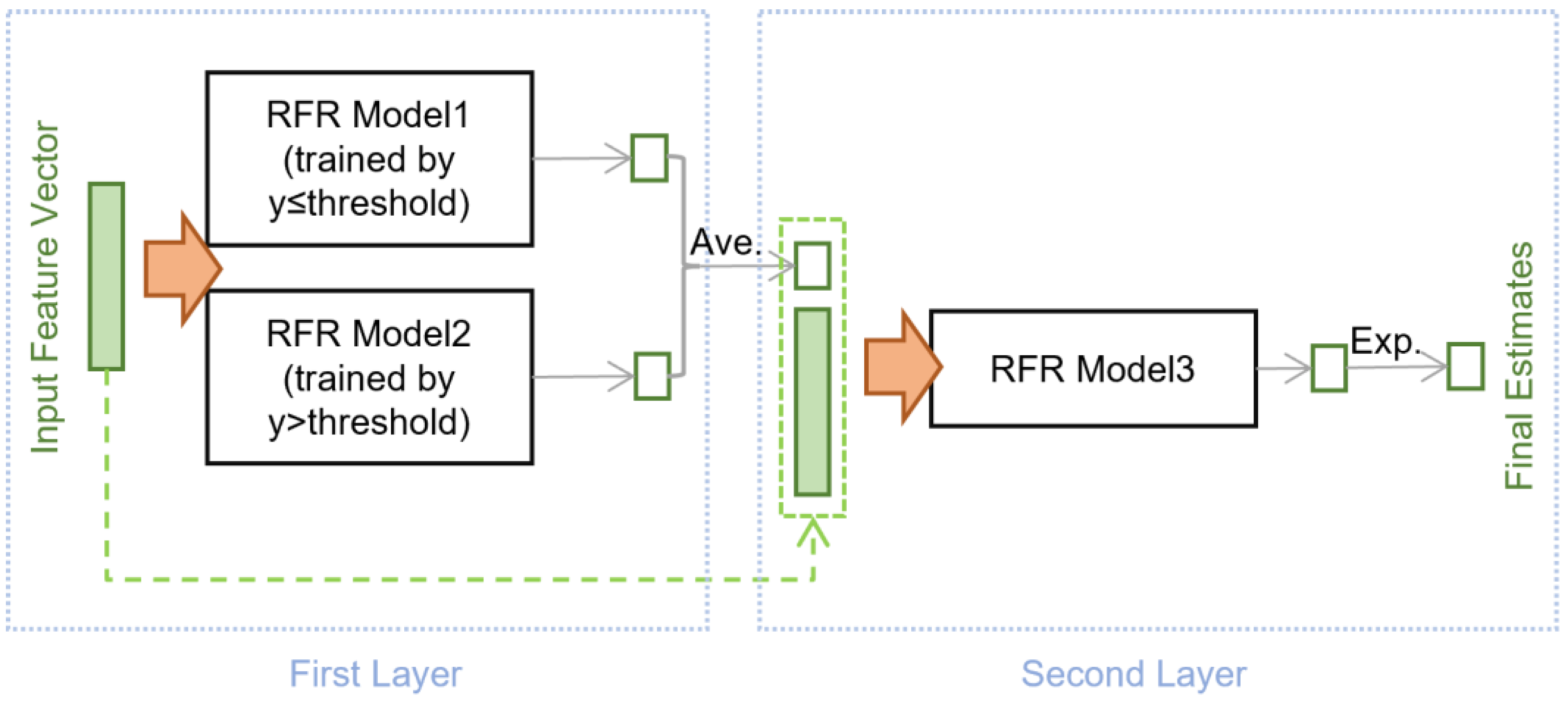
3.2. Two-Layer Stacked Random Forest Regression Model

The fossil fuel CO₂ emission values have an obviously unbalanced distribution. Taking the samples in 2014 as an example, 20.9% of the fossil fuel emissions of global samples are 0, and all samples greater than 0 after logarithmic transformation have a right-skewed distribution with a skewness coefficient [74] of −0.277 (third-order moment) (Figure 1). As compared to other machine learning models, the random forest model has a better performance on unbalanced data [75], but the unbalanced distribution of the samples will still affect the model performance, resulting in high-value underestimation and low-value overestimation in model outputs. To resolve this, this study used the two-layer stacked random forest regression model as shown in Figure 3 [76].

In the first layer, the samples were divided into two segments based on the threshold determined by enumeration, and a random forest regression model was established on each segment of the samples and then calculated the mean value of the output results of two models. Next, the mean value of the output results of two models in the first layer was used as the new input variable of the second-layer model. Finally, the output of the second layer was converted to fossil fuel CO₂ emission estimates by an exponential transformation. The first layer was segmented according to the threshold and modeled separately, which to a certain extent solved the overestimation or underestimation caused by the unbalanced distribution of emission values in a single model. The second-layer model effectively resolved the problem of the obviously inaccurate estimations from sub-models in the first layer when estimating the range not covered with the training samples, which was equivalent to weighting the output results of the first layer.

In addition to the basic hyperparameters involved in random forest, our model also included structure parameters that needed to be discussed, such as the number of the sub-models and thresholds for segmentation in the first layer as well as the number of model layers. We finally determined the optimal model structure above using multiple tests.

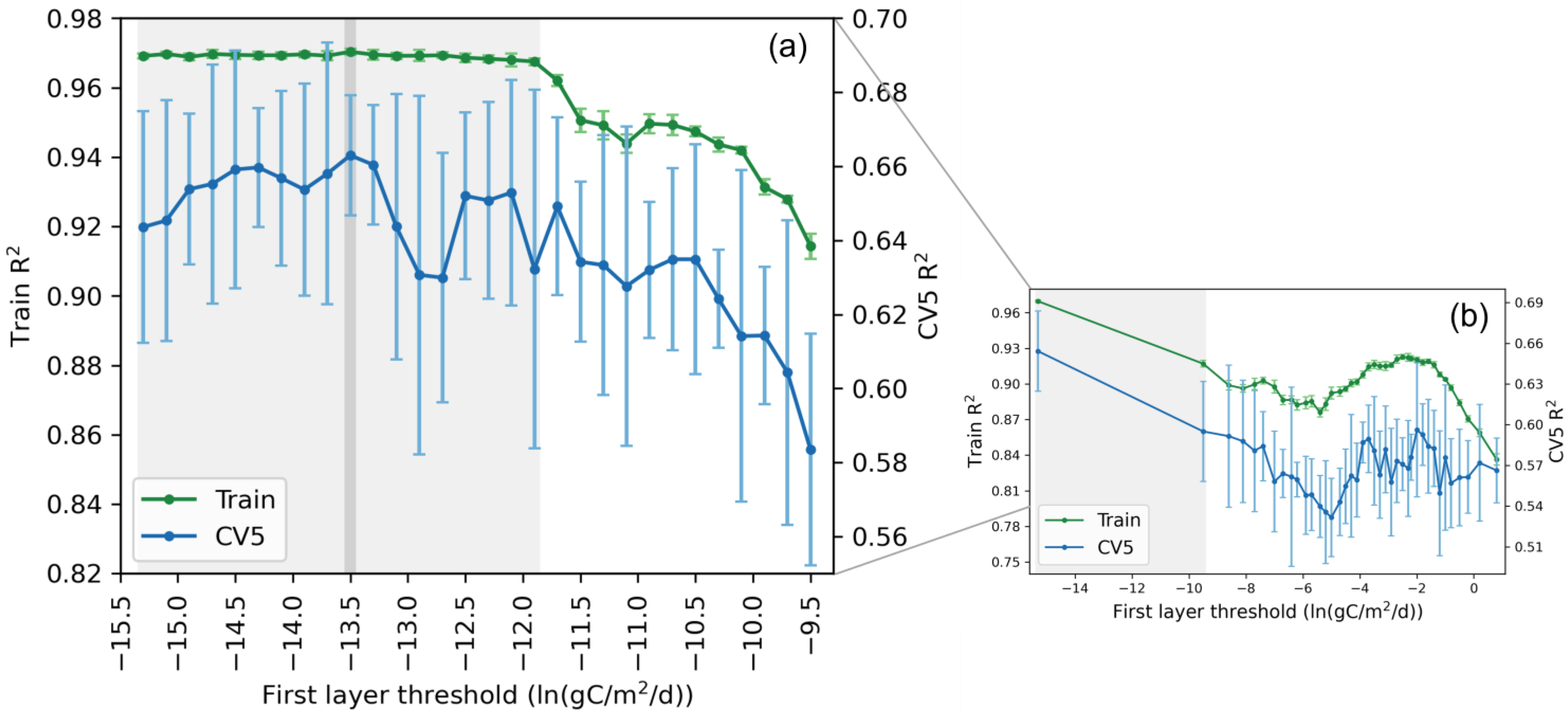
3.2.1. The Segmentation in the First Layer

For the segmentation of the first layer, we divided the model into three segments and five segments according to thresholds equaling μ ± σ and μ ± 2σ of the natural log of ODIAC in the train set, and the fitting performance on the training set of the three-segment model with R² of 0.851 ± 0.005 and RMSE of 0.276 ± 0.005 was similar to the five-segment model with R² of 0.867 ± 0.003 and RMSE of 0.261 ± 0.002, while both were inferior to the two-segment model. Then, we applied a segmentation threshold of a two-segment model from the minimum of the part greater than 0 to the maximum with a step of 2.5% of the total samples and the results of training set and 5-flod cross-validation were both used to evaluate the model. Figure 4b shows that when the threshold was between −15.3 $\left(\ln \left(\mathrm{gC}/{\mathrm{m}}^2/\mathrm{d}\right)\right)$ and −9.5 $\left(\ln \left(\mathrm{gC}/{\mathrm{m}}^2/\mathrm{d}\right)\right)$ which was the first 2.5% part of samples greater than 0, the model could have the best fitting performance according to the consistency of the two evaluation indexes. Figure 4a shows the further tests between −15.3 $\left(\ln \left(\mathrm{gC}/{\mathrm{m}}^2/\mathrm{d}\right)\right)$ and −9.5 $\left(\ln \left(\mathrm{gC}/{\mathrm{m}}^2/\mathrm{d}\right)\right)$ with the step of 0.2 $\left(\ln \left(\mathrm{gC}/{\mathrm{m}}^2/\mathrm{d}\right)\right)$ and illustrates that when the threshold was below −11.7 $\left(\ln \left(\mathrm{gC}/{\mathrm{m}}^2/\mathrm{d}\right)\right)$, the fitting performance was significantly superior to the others and not sensitive to the values. Therefore, −13.5 $\left(\ln \left(\mathrm{gC}/{\mathrm{m}}^2/\mathrm{d}\right)\right)$ was selected as the final segmentation threshold for a slightly better fitting performance than other values in that range.

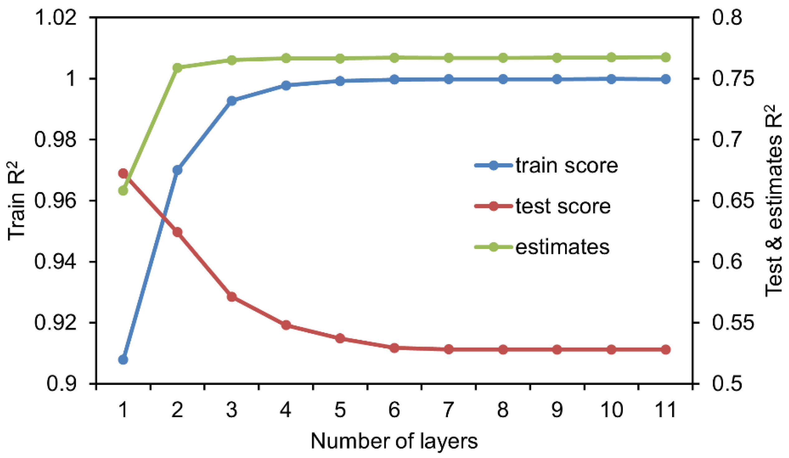
3.2.2. The Number of Model Layers

To select the optimal number of model layers, we increased the number of layers from 1 to 11 and undertook 10 independent trainings for each number (Figure 5). In a comparison of the R² of the training set, the test set, and the estimates, Figure 5 shows that when the number of layers reached 2, the accuracy of the emission estimates (the green line) was stable at a high level, and when the number of model layers exceeded 2, the train score (the blue line) and test score (the red line) appeared to plateau at a high level and a low level, respectively, which indicated that the model had been overfitted. The two-layer model had the advantage of better accuracy on emission estimates and stronger generalization performance; therefore, we adopted the two-layer model.

4. Results

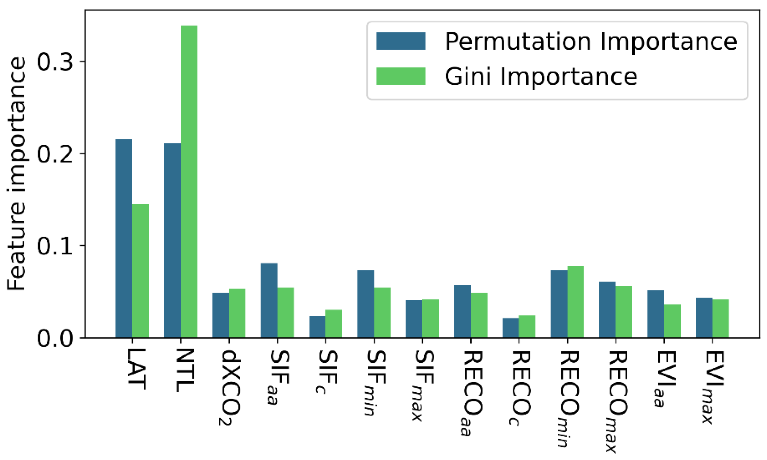
4.1. Feature Importance in the Two-Layer Stacked Model

To further understand the role of each feature in the model, we used the normalized Gini importance [77] and the normalized permutation importance [78] to describe the importance of features. The Gini importance of each feature was the sum of the two sub-models in the first layer and the second-layer model. The permutation importance is the decrease in the model score (R² on the training set is used in this research) when a single feature value is randomly shuffled and we used the average over 10 shuffles.

Figure 6 shows the two importance values for each feature in the two-layer stacked model. The contributions of DNB and LAT were dominant according to both feature importance, while the other variables were lower than those two, among which, the importance of ${\mathrm{RECO}}_{\min }$, ${\mathrm{RECO}}_{\max }$, ${\mathrm{SIF}}_{\mathrm{aa}}$, and ${\mathrm{SIF}}_{\min }$ was slightly more significant. The night-time light played a conspicuous role in the model which may be related to the NTL variable originating from the same night-time light data source as the spatial proxy of ODIAC data [79]. At the same time, the high importance of LAT may relate to distinct latitudinal geographic distribution patterns of all other features. While, neither of the two importance values of dXCO₂ from satellite observations were high. That could be due to the fact that the long lifetime of CO₂ results in the XCO₂ anomalies caused by anthropogenic CO₂ emissions are strongly disturbed by atmospheric transport and terrestrial photosynthetic activities [24] and the XCO₂ anomalies are the coupling effects of the natural carbon cycle and anthropogenic emissions, which makes it difficult to separate them [17,39]. Moreover, ${\mathrm{SIF}}_{\mathrm{c}}$ and ${\mathrm{RECO}}_{\mathrm{c}}$ were not as important as the other variables from the same data source, but their differences were small, which indicated that these timeseries terrestrial features played a complementary role in the two-layer stacked model.

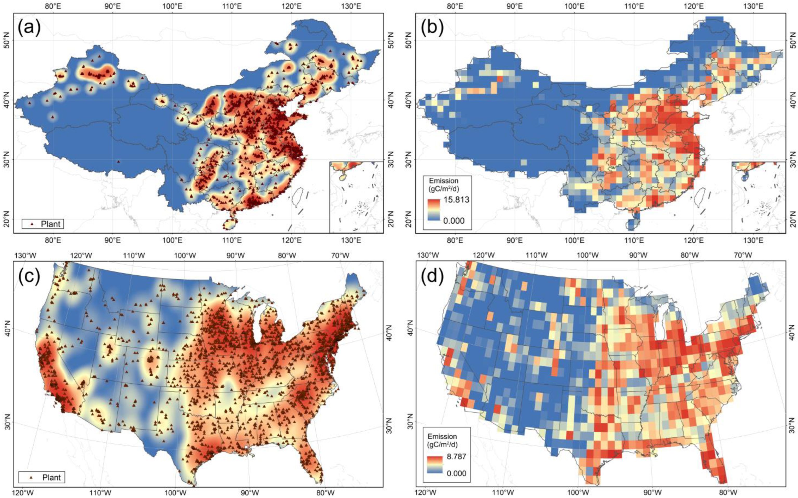
4.2. Spatial Distribution of Estimated CO₂ Emissions

The data-driven two-layer stacked random forest model was trained using the ODIAC fossil fuel CO₂ gridded emission data in 2014–2018 and tested using the 2019 dataset, and driven by the dXCO₂, VIIRS night-time light, terrestrial ecosystem carbon flux, SIF, and EVI data. Since the mapping XCO₂ data does not cover areas north of 65°N and south of 56°S, these areas were not included in the model outputs.

Figure 7 shows the annual average of gridded global fossil fuel emission estimates in 2019 (Figure 7a), the annual average of the ODIAC 1° data products in 2019 (Figure 7b), the uncertainty (Figure 7c), and the estimation error (Figure 7d). As compared to the ODIAC 1° data product (Figure 7b), the missing pixels of output results were mainly distributed in the high latitudes of the northern hemisphere where human activities were scarce and human emissions were low. Overall, the spatial distribution of the model estimation results and the ODIAC data were relatively consistent. There were high-emission areas in southeastern North America, western Europe, the Indian peninsula, and East Asia, which were in line with the distribution of high-emission areas and countries recently reported by the GCP and the Emissions Database for Global Atmospheric Research (EDGAR) [3,80]. In addition, there were continuous large low-emission areas in northern North America, Siberia, the Qinghai Tibet Plateau, most of Africa, the Amazon rainforest region, and central and western Australia, where there were fewer human activities or larger vegetation coverage, which ensured that anthropogenic carbon emissions in these areas were significantly lower than in other regions. The difference in the spatial distribution between the model estimates and the ODIAC was related to the medium-emission and high-emission areas of the model having a more obvious boundary, while in the ODIAC data, these areas were more fragmented, which indicated the model underestimating the high-emission regions distribution in the low-emission accumulation areas. The estimation errors were concentrated around 0 (Figure 7d), and 49.9% of them were lower than 0, which indicated that the numbers of overestimated and underestimated pixels were similar.

4.3. Validation of Emission Estimates

4.3.1. Validation Using the Test Set

Generally, our emission estimates had a similar histogram distribution with ODIAC (Figure 8a). In addition, Figure 8b shows the correlation between our gridded emission estimates and the annual mean of the ODIAC 1° data product in 2019. The R² between them reached 0.766, and the RMSE was 0.359 on a global scale. Our two-layer structure improved the accuracy on emission estimates by 16.4% as compared to the single random forest regression model (R² = 0.658 ± 0.007, RMSE = 0.434 ± 0.004; Figure 5), and the R² of the high-emission samples that were greater than the threshold increased by 17.3% (increased from 0.649 to 0.761), and the RMSE decreased from 0.489 to 0.404.

To further verify the model estimates, we estimated the total emission of each country under sinusoidal projection. Limited by the 1° × 1° spatial resolution, the countries with too small an area (the area of a single pixel was 2470${\mathrm{km}}^2$) were excluded from the total emission calculation; in addition, the countries involving the areas north of 65°N were also excluded due to having no data pixels in the gridded emission estimates. In the end, we obtained emissions from 140 countries. The national emissions estimated by the model were highly consistent with those estimated by 1° ODIAC data, and their R² was 0.991 (Figure 9), which illustrated that from grid level to country level, the correlation between them increased significantly as the scale became thicker.

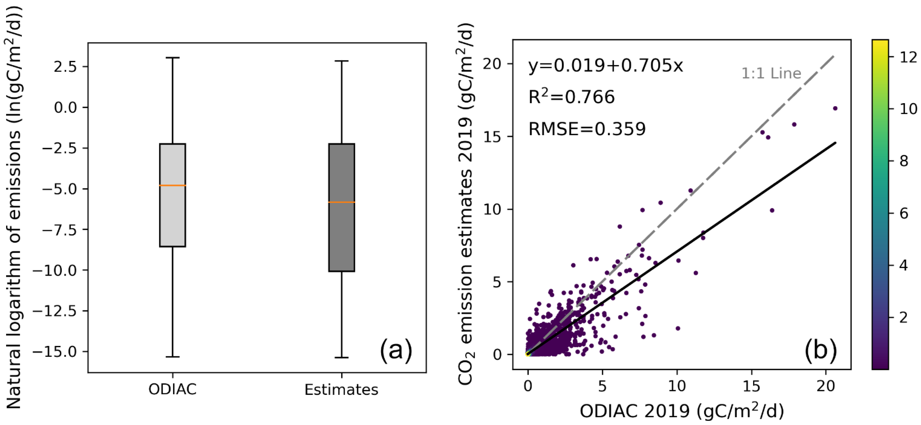
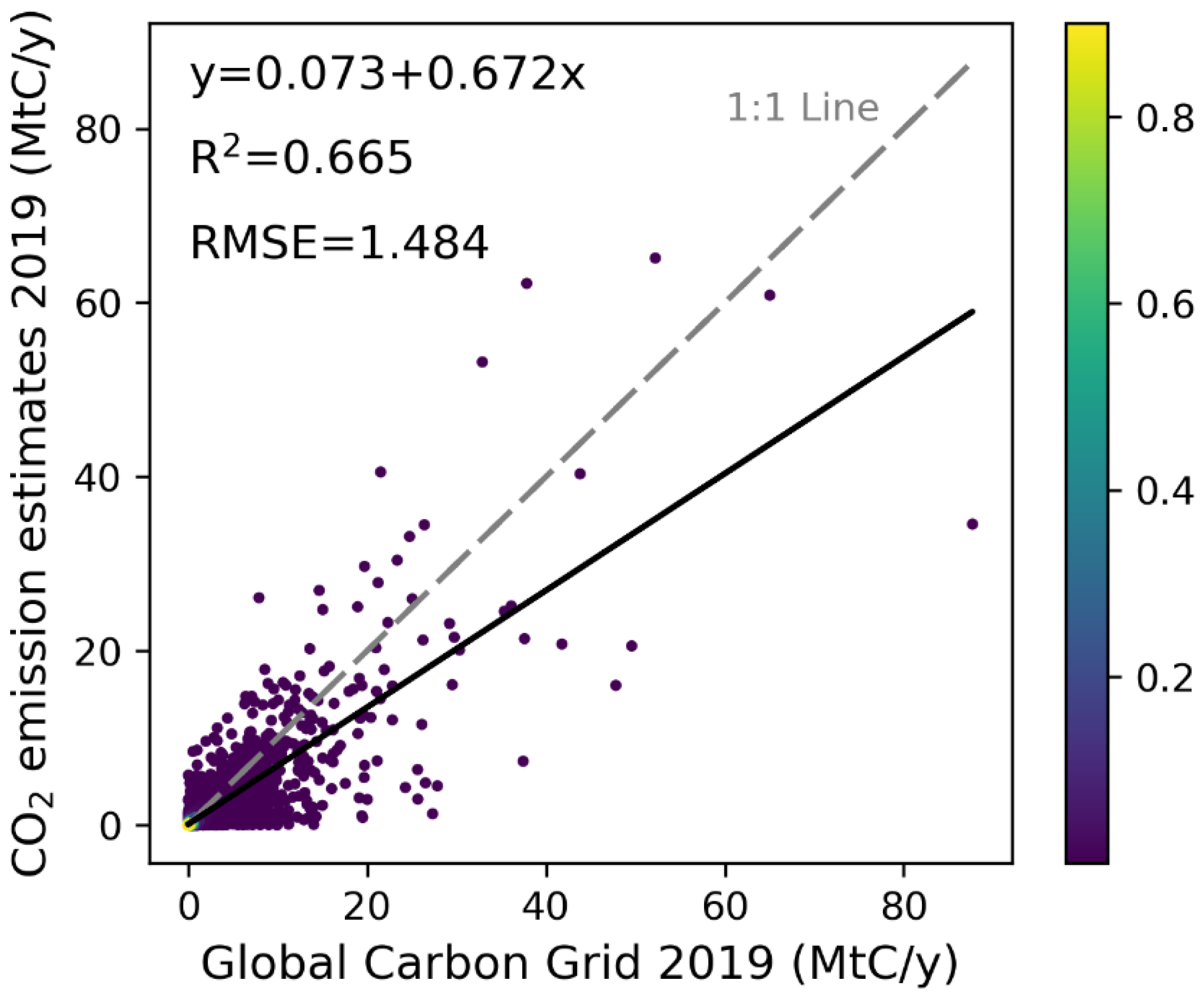
4.3.2. Validation Using the Third-Party Emission Dataset

We undertook a third-party validation at the 1° gridded scale (Figure 10) using Global Carbon Grid emission data [49] from the Global Infrastructure Emission Database (GID). Figure 10 illustrated a close correlation between our emissions and Global Carbon Grid with an R² of 0.665.

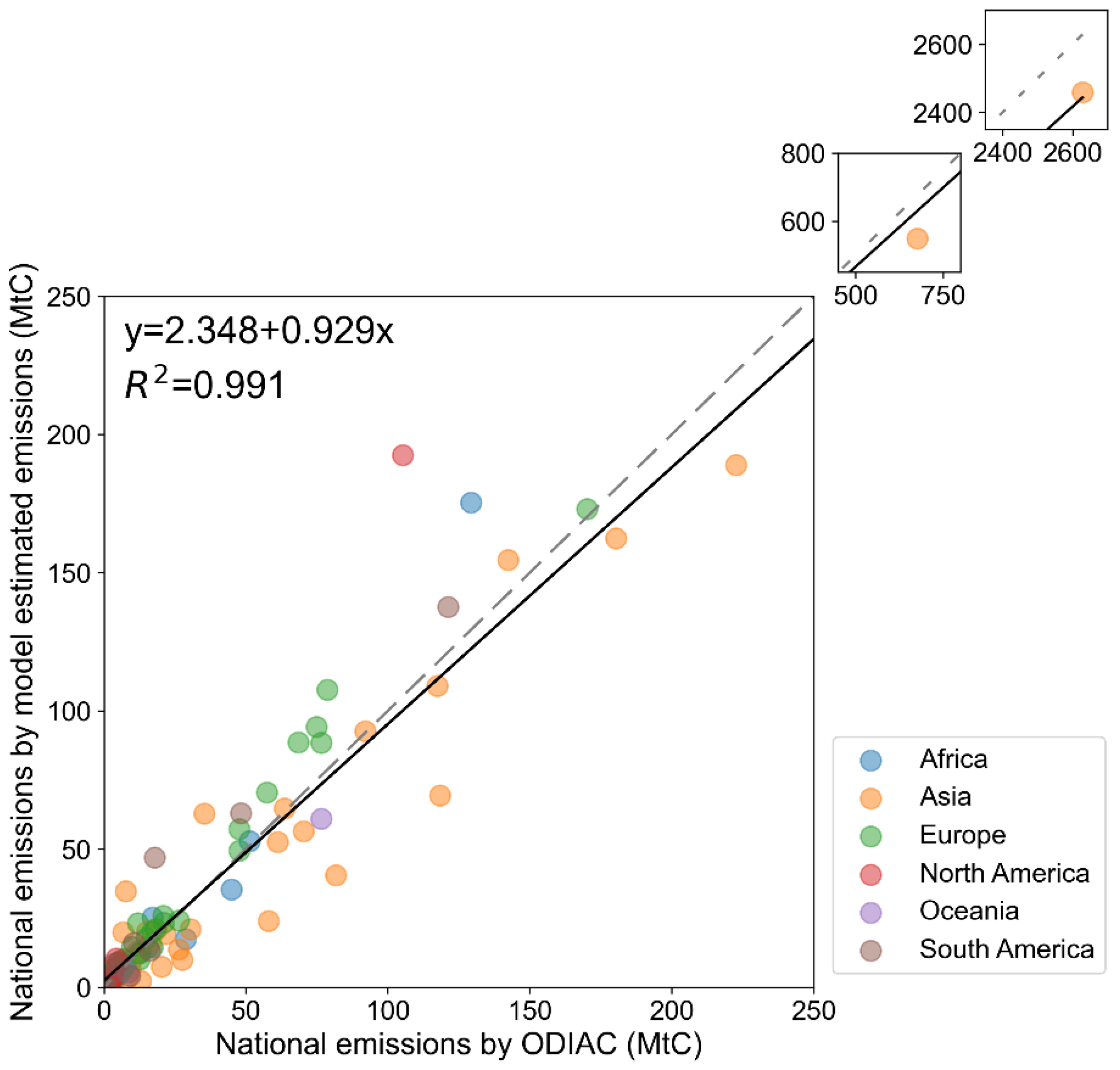
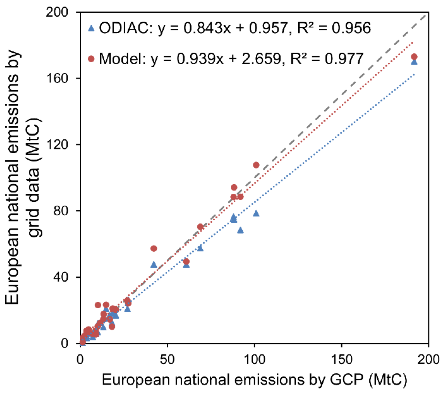
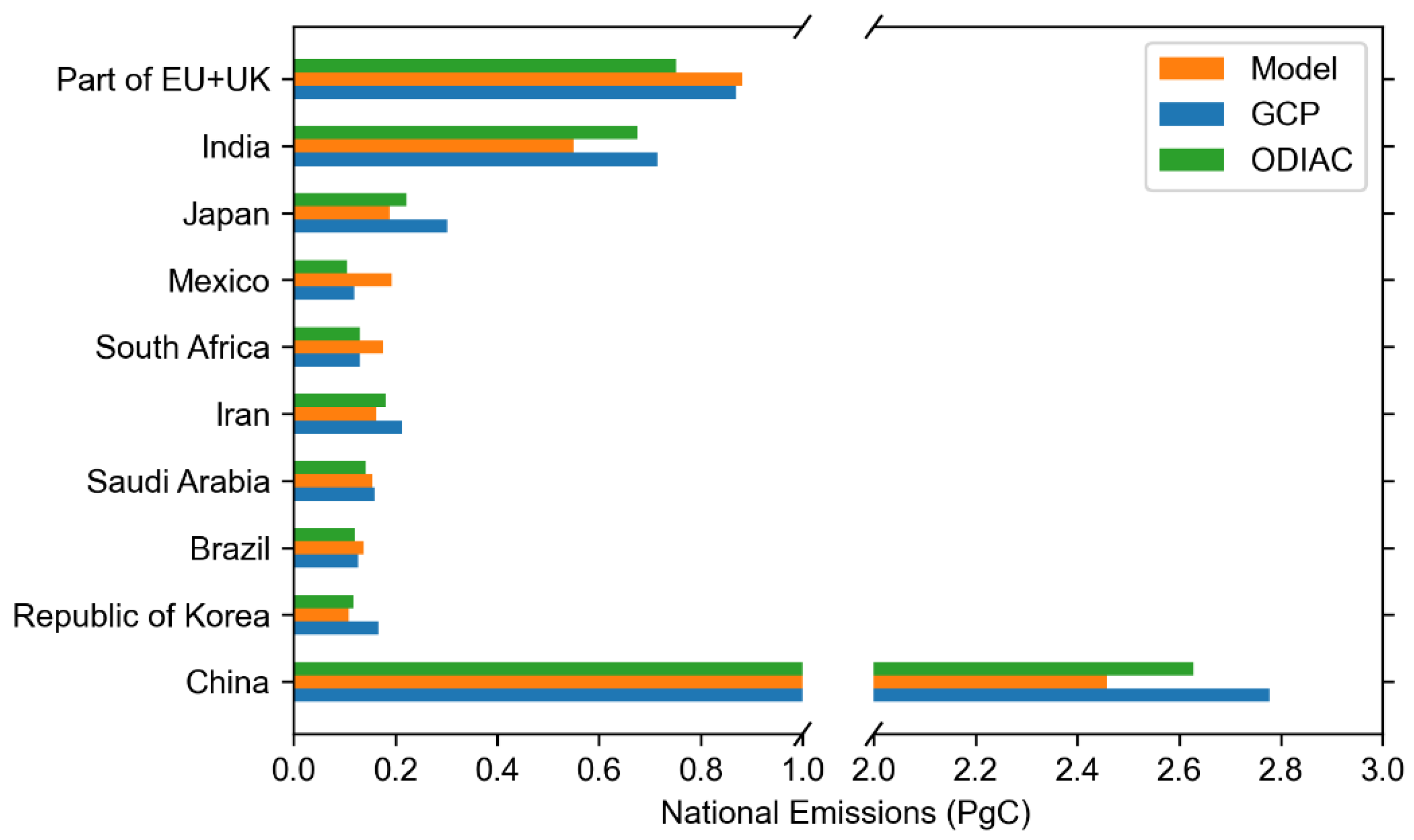
4.4. Consistency with GCP National CO₂ Emissions

We compared the national emissions calculated by two types of grid data (emission estimates using our model and the ODIAC) and the inventory results from the GCP [51]. The results suggested that among the 140 countries calculated by model estimates, European national emissions were more consistent with the GCP results (Figure 11) than the ODIAC, for the R² with the GCP results (R² = 0.977) was 2.2% higher than the ODIAC (R² = 0.956). This was attributed to European countries having denser impervious surfaces compared with the other countries [63] and the impervious surfaces were highly correlated with night-time light of which the feature importance was higher in this model.

Figure 12 shows the top 10 national or regional emissions in 2019 out of 140 countries estimated by the model. We did not include Cyprus, Luxembourg, Malta, Finland, and Sweden in the European Union countries as their areas were either not large enough or involving north of 65°N. Comparing the national or regional emissions of the three data sources, it can be found that the national emissions estimated by our model were significantly lower in China and India than in the other two data sources. China’s emissions in 2019 were estimated at 2.46 PgC, which was 11.5% lower than the GCP data (2.78 PgC) and 6.5% lower than the ODIAC data (2.63 PgC); India was estimated at 0.55 PgC, which was 23% lower than the GCP data (0.71 PgC) and 19% lower than the ODIAC data (0.68 PgC). In comparison, the model estimates were higher than the other two data sources in Mexico (the model estimate was 1.92 PgC, where the GCP was 1.20 PgC and the ODIAC was 1.05 PgC) and South Africa (the model estimate was 1.75 PgC, where the GCP was 1.31 PgC and the ODIAC was 1.29 PgC).

At the same time, the product with 1° spatial resolution was not enough to support the estimation of the total emissions for a country or region, especially in a small area. This model has a great potential to achieve high spatial and temporal resolution estimations of anthropogenic carbon emissions with the continuous improvement of remote sensing satellites for monitoring atmospheric compositions, which will increase the number and scope of available samples and refine the sample grid globally.

5. Discussion

We further compared the spatial distribution of our gridded emissions with fossil fuel fired power plants which are the hot spots of CO₂ emissions [81] in Mainland China (Figure 13a,b) and the contiguous United States (Figure 13c,d). The power plants data of Mainland China was from the Global Coal Plant Tracker [82] and Global Gas Plant Tracker [83] of the Global Energy Monitor (GEM). The power plants data of the contiguous United States in 2019 was from the emissions and generation resource integrated database (eGRID) which was developed by the Clean Air Markets Division of the United States Environmental Protection Agency (EPA). Our emission estimates are highly consistent with the spatial distribution of power plants both in Mainland China and the contiguous United States that the power plant clusters are covered with the high emission pixels, which means our gridded emission estimates can reflect the distribution of the large emission sources. Moreover, it is worth noting that power plants are located in almost all the emission area of the gridded emission map. According to the Carbon Monitor data [9], in 2019, the power sector contributed 43.5% of the national total emissions in China, ranking first, and the ratio is 31.4% in the US which is the second out of the six sectors, 0.8% less than the first. The prominent emissions contribution of the power sector in both regions may account for this overlap in spatial distribution.

6. Conclusions

The accurate estimation of anthropogenic carbon emissions is fundamental to understanding the global carbon cycle process and supporting the setting and implementation of CO₂ emission-reduction goals. This study built a two-layer data-driven stacked random forest regression model to estimate fossil fuel CO₂ emissions at a 1° grid scale. Among the driving features, night-time light and latitude contributed the most to the model, followed by ecosystem respiration and SIF. The validation on the test set showed a consistency between our gridded emission estimates and ODIAC data in spatial distribution, and the two-layer stacked random forest regression model improved the accuracy as compared to the single-layer model with an R² of 0.766 and an RMSE of 0.359. The cross-validation using third-party datasets of Global Carbon Grid and Carbon Monitor illustrated that our gridded emission map in 2019 was credible with an R² of 0.665. At a national scale, the emissions calculated by our model estimates were consistent with the national emissions reported by the GCP with an R² of 0.977, which was 2.2% higher than that between the GCP and the ODIAC data in European countries. This study provides a new approach for estimating global anthropogenic carbon emissions at grid scale.

References

1. Stocker, T.F.; Qin, D.; Plattner, G.-K.; Tignor, M.; Allen, S.K.; Boschung, J.; Nauels, A.; Xia, Y.; Bex, V.; Midgley, P.M. (Eds.) Carbon and Other Biogeochemical Cycles. In Climate Change 2013: The Physical Science Basis. Contribution of Working Group I to the Fifth Assessment Report of the Intergovernmental Panel on Climate Change; Cambridge University Press: Cambridge, UK, 2014; pp. 465–570. [Google Scholar]
2. Friedlingstein, P.; Jones, M.W.; O’Sullivan, M.; Andrew, R.M.; Bakker, D.C.E.; Hauck, J.; Le Quéré, C.; Peters, G.P.; Peters, W.; Pongratz, J.; et al. Global Carbon Budget 2021. Earth Syst. Sci. Data Discuss. 2021, 2021, 1–191. [Google Scholar] [CrossRef]
3. Friedlingstein, P.; O’Sullivan, M.; Jones, M.W.; Andrew, R.M.; Hauck, J.; Olsen, A.; Peters, G.P.; Peters, W.; Pongratz, J.; Sitch, S.; et al. Global Carbon Budget 2020. Earth Syst. Sci. Data 2020, 12, 3269–3340. [Google Scholar] [CrossRef]
4. Nations, U. Paris Agreement. 2015. Available online: https://unfccc.int/files/essential_background/convention/application/pdf/english_paris_agreement.pdf (accessed on 30 March 2022).
5. Le Quéré, C.; Korsbakken, J.I.; Wilson, C.; Tosun, J.; Andrew, R.; Andres, R.J.; Canadell, J.G.; Jordan, A.; Peters, G.P.; van Vuuren, D.P. Drivers of declining CO2 emissions in 18 developed economies. Nat. Clim. Change 2019, 9, 213–217. [Google Scholar] [CrossRef]
6. Rogelj, J.; den Elzen, M.; Höhne, N.; Fransen, T.; Fekete, H.; Winkler, H.; Schaeffer, R.; Sha, F.; Riahi, K.; Meinshausen, M. Paris Agreement climate proposals need a boost to keep warming well below 2 °C. Nature 2016, 534, 631–639. [Google Scholar] [CrossRef] [PubMed]
7. Ballantyne, A.P.; Alden, C.B.; Miller, J.B.; Tans, P.P.; White, J.W.C. Increase in observed net carbon dioxide uptake by land and oceans during the past 50 years. Nature 2012, 488, 70–72. [Google Scholar] [CrossRef] [PubMed]
8. Zheng, B.; Cheng, J.; Geng, G.; Wang, X.; Li, M.; Shi, Q.; Qi, J.; Lei, Y.; Zhang, Q.; He, K. Mapping anthropogenic emissions in China at 1 km spatial resolution and its application in air quality modeling. Sci. Bull. 2021, 66, 612–620. [Google Scholar] [CrossRef]
9. Liu, Z.; Ciais, P.; Deng, Z.; Davis, S.J.; Zheng, B.; Wang, Y.; Cui, D.; Zhu, B.; Dou, X.; Ke, P.; et al. Carbon Monitor, a near-real-time daily dataset of global CO2 emission from fossil fuel and cement production. Sci. Data 2020, 7, 392. [Google Scholar] [CrossRef] [PubMed]
10. Andres, R.; Boden, T.; Higdon, D. A new evaluation of the uncertainty associated with CDIAC estimates of fossil fuel carbon dioxide emission. Tellus B 2014, 66, 23616. [Google Scholar] [CrossRef]
11. Andres, R.J.; Boden, T.A.; Bréon, F.M.; Ciais, P.; Davis, S.; Erickson, D.; Gregg, J.S.; Jacobson, A.; Marland, G.; Miller, J.; et al. A synthesis of carbon dioxide emissions from fossil-fuel combustion. Biogeosciences 2012, 9, 1845–1871. [Google Scholar] [CrossRef]
12. Andres, R.J.; Boden, T.A.; Higdon, D.M. Gridded uncertainty in fossil fuel carbon dioxide emission maps, a CDIAC example. Atmos. Chem. Phys. 2016, 16, 14979–14995. [Google Scholar]
13. Sargent, M.; Barrera, Y.; Nehrkorn, T.; Hutyra, L.R.; Gately, C.K.; Jones, T.; McKain, K.; Sweeney, C.; Hegarty, J.; Hardiman, B.; et al. Anthropogenic and biogenic CO2 fluxes in the Boston urban region. Proc. Natl. Acad. Sci. USA 2018, 115, 7491. [Google Scholar] [CrossRef]
14. Janardanan, R.; Maksyutov, S.; Oda, T.; Saito, M.; Kaiser, J.W.; Ganshin, A.; Stohl, A.; Matsunaga, T.; Yoshida, Y.; Yokota, T. Comparing GOSAT observations of localized CO2 enhancements by large emitters with inventory-based estimates. Geophys. Res. Lett. 2016, 43, 3486–3493. [Google Scholar] [CrossRef]
15. Bovensmann, H.; Buchwitz, M.; Burrows, J.P.; Reuter, M.; Krings, T.; Gerilowski, K.; Schneising, O.; Heymann, J.; Tretner, A.; Erzinger, J. A remote sensing technique for global monitoring of power plant CO2 emissions from space and related applications. Atmos. Meas. Tech. 2010, 3, 781–811. [Google Scholar] [CrossRef]
16. Newman, S.; Xu, X.; Gurney, K.R.; Hsu, Y.K.; Li, K.F.; Jiang, X.; Keeling, R.; Feng, S.; O’Keefe, D.; Patarasuk, R.; et al. Toward consistency between trends in bottom-up CO2 emissions and top-down atmospheric measurements in the Los Angeles megacity. Atmos. Chem. Phys. 2016, 16, 3843–3863. [Google Scholar] [CrossRef]
17. Chevallier, F.; Palmer, P.I.; Feng, L.; Boesch, H.; O’Dell, C.W.; Bousquet, P. Toward robust and consistent regional CO2 flux estimates from in situ and spaceborne measurements of atmospheric CO2. Geophys. Res. Lett. 2014, 41, 1065–1070. [Google Scholar] [CrossRef]
18. Detmers, R.G.; Hasekamp, O.; Aben, I.; Houweling, S.; van Leeuwen, T.T.; Butz, A.; Landgraf, J.; Köhler, P.; Guanter, L.; Poulter, B. Anomalous carbon uptake in Australia as seen by GOSAT. Geophys. Res. Lett. 2015, 42, 8177–8184. [Google Scholar] [CrossRef]
19. Wang, H.; Jiang, F.; Liu, Y.; Yang, D.; Wu, M.; He, W.; Wang, J.; Wang, J.; Ju, W.; Chen, J.M. Global Terrestrial Ecosystem Carbon Flux Inferred from TanSat XCO2 Retrievals. J. Remote Sens. 2022, 2022, 9816536. [Google Scholar] [CrossRef]
20. Eldering, A.; Wennberg, P.O.; Crisp, D.; Schimel, D.S.; Gunson, M.R.; Chatterjee, A.; Liu, J.; Schwandner, F.M.; Sun, Y.; O’Dell, C.W.; et al. The Orbiting Carbon Observatory-2 early science investigations of regional carbon dioxide fluxes. Science 2017, 358, eaam5745. [Google Scholar] [CrossRef] [PubMed]
21. Eldering, A.; Taylor, T.E.; O’Dell, C.W.; Pavlick, R. The OCO-3 mission: Measurement objectives and expected performance based on 1 year of simulated data. Atmos. Meas. Tech. 2019, 12, 2341–2370. [Google Scholar] [CrossRef]
22. Yokota, T.; Yoshida, Y.; Eguchi, N.; Ota, Y.; Tanaka, T.; Watanabe, H.; Maksyutov, S.J.S. Global Concentrations of CO2 and CH4 Retrieved from GOSAT: First Preliminary Results. SOLA 2009, 5, 160–163. [Google Scholar] [CrossRef]
23. Yang, D.; Boesch, H.; Liu, Y.; Somkuti, P.; Cai, Z.; Chen, X.; Di Noia, A.; Lin, C.; Lu, N.; Lyu, D.; et al. Toward High Precision XCO2 Retrievals from TanSat Observations: Retrieval Improvement and Validation Against TCCON Measurements. J. Geophys. Res. Atmos. 2020, 125, e2020JD032794. [Google Scholar] [CrossRef] [PubMed]
24. Hakkarainen, J.; Ialongo, I.; Tamminen, J. Direct space-based observations of anthropogenic CO2 emission areas from OCO-2. Geophys. Res. Lett. 2016, 43, 11, 400-11, 406. [Google Scholar] [CrossRef]
25. Schwandner Florian, M.; Gunson Michael, R.; Miller Charles, E.; Carn Simon, A.; Eldering, A.; Krings, T.; Verhulst Kristal, R.; Schimel David, S.; Nguyen Hai, M.; Crisp, D.; et al. Spaceborne detection of localized carbon dioxide sources. Science 2017, 358, eaam5782. [Google Scholar] [CrossRef] [PubMed]
26. Schneising, O.; Heymann, J.; Buchwitz, M.; Reuter, M.; Bovensmann, H.; Burrows, J.P. Anthropogenic carbon dioxide source areas observed from space: Assessment of regional enhancements and trends. Atmos. Chem. Phys. 2013, 13, 2445–2454. [Google Scholar] [CrossRef]
27. Kiel, M.; Eldering, A.; Roten, D.D.; Lin, J.C.; Feng, S.; Lei, R.; Lauvaux, T.; Oda, T.; Roehl, C.M.; Blavier, J.-F.; et al. Urban-focused satellite CO2 observations from the Orbiting Carbon Observatory-3: A first look at the Los Angeles megacity. Remote Sens. Environ. 2021, 258, 112314. [Google Scholar] [CrossRef]
28. Buchwitz, M.; Reuter, M.; Noël, S.; Bramstedt, K.; Schneising, O.; Hilker, M.; Fuentes Andrade, B.; Bovensmann, H.; Burrows, J.P.; Di Noia, A.; et al. Can a regional-scale reduction of atmospheric CO2 during the COVID-19 pandemic be detected from space? A case study for East China using satellite XCO2 retrievals. Atmos. Meas. Tech. 2021, 14, 2141–2166. [Google Scholar] [CrossRef]
29. Belgiu, M.; Drăguţ, L. Random forest in remote sensing: A review of applications and future directions. ISPRS J. Photogramm. Remote Sens. 2016, 114, 24–31. [Google Scholar] [CrossRef]
30. Tramontana, G.; Jung, M.; Schwalm, C.R.; Ichii, K.; Camps-Valls, G.; Ráduly, B.; Reichstein, M.; Arain, M.A.; Cescatti, A.; Kiely, G.; et al. Predicting carbon dioxide and energy fluxes across global FLUXNET sites with regression algorithms. Biogeosciences 2016, 13, 4291–4313. [Google Scholar] [CrossRef]
31. Mahdianpari, M.; Salehi, B.; Mohammadimanesh, F.; Motagh, M. Random forest wetland classification using ALOS-2 L-band, RADARSAT-2 C-band, and TerraSAR-X imagery. ISPRS J. Photogramm. Remote Sens. 2017, 130, 13–31. [Google Scholar] [CrossRef]
32. Wen, L.; Cao, Y. Influencing factors analysis and forecasting of residential energy-related CO2 emissions utilizing optimized support vector machine. J. Clean. Prod. 2020, 250, 119492. [Google Scholar] [CrossRef]
33. Leerbeck, K.; Bacher, P.; Junker, R.G.; Goranović, G.; Corradi, O.; Ebrahimy, R.; Tveit, A.; Madsen, H. Short-term forecasting of CO2 emission intensity in power grids by machine learning. Appl. Energy 2020, 277, 115527. [Google Scholar] [CrossRef]
34. Magazzino, C.; Mele, M.; Schneider, N. A machine learning approach on the relationship among solar and wind energy production, coal consumption, GDP, and CO2 emissions. Renew. Energy 2021, 167, 99–115. [Google Scholar] [CrossRef]
35. Yang, S.; Lei, L.; Zeng, Z.; He, Z.; Zhong, H. An Assessment of Anthropogenic CO2 Emissions by Satellite-Based Observations in China. Sensors 2019, 19, 1118. [Google Scholar] [CrossRef] [PubMed]
36. Mustafa, F.; Bu, L.; Wang, Q.; Yao, N.; Shahzaman, M.; Bilal, M.; Aslam, R.W.; Iqbal, R. Neural-network-based estimation of regional-scale anthropogenic CO2 emissions using an Orbiting Carbon Observatory-2 (OCO-2) dataset over East and West Asia. Atmos. Meas. Tech. 2021, 14, 7277–7290. [Google Scholar] [CrossRef]
37. Kohavi, R.; John, G.H. Wrappers for feature subset selection. Artif. Intell. 1997, 97, 273–324. [Google Scholar] [CrossRef]
38. Guyon, I.; Elisseeff, A. An introduction to variable and feature selection. J. Mach. Learn. Res. 2003, 3, 1157–1182. [Google Scholar]
39. Ye, X.; Lauvaux, T.; Kort, E.A.; Oda, T.; Feng, S.; Lin, J.C.; Yang, E.G.; Wu, D. Constraining Fossil Fuel CO2 Emissions from Urban Area Using OCO-2 Observations of Total Column CO2. J. Geophys. Res. Atmos. 2020, 125, e2019JD030528. [Google Scholar] [CrossRef]
40. Janssens-Maenhout, G.; Crippa, M.; Guizzardi, D.; Muntean, M.; Schaaf, E.; Dentener, F.; Bergamaschi, P.; Pagliari, V.; Olivier, J.G.J.; Peters, J.A.H.W.; et al. EDGAR v4.3.2 Global Atlas of the three major greenhouse gas emissions for the period 1970–2012. Earth Syst. Sci. Data 2019, 11, 959–1002. [Google Scholar] [CrossRef]
41. Andrew, R.M. A comparison of estimates of global carbon dioxide emissions from fossil carbon sources. Earth Syst. Sci. Data 2020, 12, 1437–1465. [Google Scholar] [CrossRef]
42. Gurney, K.R.; Liang, J.; O’Keeffe, D.; Patarasuk, R.; Hutchins, M.; Huang, J.; Rao, P.; Song, Y. Comparison of Global Downscaled Versus Bottom-Up Fossil Fuel CO2 Emissions at the Urban Scale in Four U.S. Urban Areas. J. Geophys. Res. Atmos. 2019, 124, 2823–2840. [Google Scholar] [CrossRef]
43. Fu, P.; Xie, Y.; Moore, C.E.; Myint, S.W.; Bernacchi, C.J. A Comparative Analysis of Anthropogenic CO2 Emissions at City Level Using OCO-2 Observations: A Global Perspective. Earths Future 2019, 7, 1058–1070. [Google Scholar] [CrossRef]
44. Wang, Y.; Ciais, P.; Broquet, G.; Bréon, F.M.; Oda, T.; Lespinas, F.; Meijer, Y.; Loescher, A.; Janssens-Maenhout, G.; Zheng, B.; et al. A global map of emission clumps for future monitoring of fossil fuel CO2 emissions from space. Earth Syst. Sci. Data 2019, 11, 687–703. [Google Scholar] [CrossRef]
45. Crowell, S.; Baker, D.; Schuh, A.; Basu, S.; Jacobson, A.R.; Chevallier, F.; Liu, J.; Deng, F.; Feng, L.; McKain, K.; et al. The 2015–2016 carbon cycle as seen from OCO-2 and the global in situ network. Atmos. Chem. Phys. 2019, 19, 9797–9831. [Google Scholar] [CrossRef]
46. Oda, T.; Maksyutov, S.; Andres, R.J. The Open-source Data Inventory for Anthropogenic CO2, version 2016 (ODIAC2016): A global monthly fossil fuel CO2 gridded emissions data product for tracer transport simulations and surface flux inversions. Earth Syst. Sci. Data 2018, 10, 87–107. [Google Scholar] [CrossRef] [PubMed]
47. Tomohiro, O.; Shamil, M. ODIAC Fossil Fuel CO2 Emissions Dataset, Center for Global Environmental Research, National Institute for Environmental Studies, ODIAC2020b. NIES 2015. [Google Scholar] [CrossRef]
48. Tong, D.; Zhang, Q.; Zheng, Y.; Caldeira, K.; Shearer, C.; Hong, C.; Qin, Y.; Davis, S.J. Committed emissions from existing energy infrastructure jeopardize 1.5 °C climate target. Nature 2019, 572, 373–377. [Google Scholar] [CrossRef]
49. Global Energy Infrastructure Emissions Database. 2021. Available online: http://gidmodel.org.cn/ (accessed on 17 June 2022).
50. Dou, X.; Wang, Y.; Ciais, P.; Chevallier, F.; Davis, S.J.; Crippa, M.; Janssens-Maenhout, G.; Guizzardi, D.; Solazzo, E.; Yan, F.; et al. Near-real-time global gridded daily CO2 emissions. Innovation 2022, 3, 100182. [Google Scholar] [CrossRef]
51. Project, G.C. Supplemental Data of Global Carbon Budget 2021, Global Carbon Project, Version 1.0; 2021. Available online: http://10.18160/gcp-2021 (accessed on 9 March 2022).
52. Broquet, G.; Bréon, F.M.; Renault, E.; Buchwitz, M.; Reuter, M.; Bovensmann, H.; Chevallier, F.; Wu, L.; Ciais, P. The potential of satellite spectro-imagery for monitoring CO2 emissions from large cities. Atmos. Meas. Tech. 2018, 11, 681–708. [Google Scholar] [CrossRef]
53. Sheng, M.; Lei, L.; Zeng, Z.-C.; Rao, W.; Song, H.; Wu, C. Global land 1° mapping XCO2 dataset using satellite observations of GOSAT and OCO-2 from 2009 to 2020. Big Earth Data 2021. Harvard Dataverse, V4. Available online: http://10.7910/DVN/4WDTD8 (accessed on 9 March 2022).
54. Randerson, J.T.; Thompson, M.V.; Conway, T.J.; Fung, I.Y.; Field, C.B. The contribution of terrestrial sources and sinks to trends in the seasonal cycle of atmospheric carbon dioxide. Glob. Biogeochem. Cycles 1997, 11, 535–560. [Google Scholar] [CrossRef]
55. FAO; Aaron, A.B.R.; Gibbs, H.K. Global Ecofloristic Zones Mapped by the United Nations Food and Agricultural Organization. 2008. Available online: https://databasin.org/datasets/dc4f6efd1fa84ea99df61ae9c5b3b763/ (accessed on 14 January 2022).
56. Stephen, M.; Stephanie, W.; Calvin, L. VIIRS day/night band (DNB) stray light characterization and correction. In Proceedings of the SPIE, San Diego, CA, USA, 25–29 August 2013. [Google Scholar]
57. Bennett, M.M.; Smith, L.C. Advances in using multitemporal night-time lights satellite imagery to detect, estimate, and monitor socioeconomic dynamics. Remote Sens. Environ. 2017, 192, 176–197. [Google Scholar] [CrossRef]
58. Zeng, J. A Data-Driven Upscale Product of Global Gross Primary Production, Net Ecosystem Exchange and Ecosystem Respiration; Center for Global Environmental Research, National Institute for Environmental Studies. 2020. Available online: http://10.17595/20200227.001 (accessed on 9 March 2022).
59. Li, X.; Xiao, J. A Global, 0.05-Degree Product of Solar-Induced Chlorophyll Fluorescence Derived from OCO-2, MODIS, and Reanalysis Data. Remote Sens. 2019, 11, 517. [Google Scholar] [CrossRef]
60. Zeng, J.; Matsunaga, T.; Tan, Z.-H.; Saigusa, N.; Shirai, T.; Tang, Y.; Peng, S.; Fukuda, Y. Global terrestrial carbon fluxes of 1999–2019 estimated by upscaling eddy covariance data with a random forest. Sci. Data 2020, 7, 313. [Google Scholar] [CrossRef] [PubMed]
61. Schneising, O.; Reuter, M.; Buchwitz, M.; Heymann, J.; Bovensmann, H.; Burrows, J.P. Terrestrial carbon sink observed from space: Variation of growth rates and seasonal cycle amplitudes in response to interannual surface temperature variability. Atmos. Chem. Phys. 2014, 14, 133–141. [Google Scholar] [CrossRef]
62. Basu, S.; Lehman, S.J.; Miller, J.B.; Andrews, A.E.; Sweeney, C.; Gurney, K.R.; Xu, X.; Southon, J.; Tans, P.P. Estimating US fossil fuel CO2 emissions from measurements of 14C in atmospheric CO2. Proc. Natl. Acad. Sci. USA 2020, 117, 13300–13307. [Google Scholar] [CrossRef] [PubMed]
63. Zhang, X.; Liu, L.Y.; Wu, C.S.; Chen, X.D.; Gao, Y.; Xie, S.; Zhang, B. Development of a global 30 m impervious surface map using multisource and multitemporal remote sensing datasets with the Google Earth Engine platform. Earth Syst. Sci. Data 2020, 12, 1625–1648. [Google Scholar] [CrossRef]
64. Chen, H.; Wu, B.; Yu, B.; Chen, Z.; Wu, Q.; Lian, T.; Wang, C.; Li, Q.; Wu, J. A New Method for Building-Level Population Estimation by Integrating LiDAR, Nighttime Light, and POI Data. J. Remote Sens. 2021, 2021, 9803796. [Google Scholar] [CrossRef]
65. Raupach, M.; Rayner, P.; Paget, M. Regional variations in spatial structure of nightlights, population density and fossil-fuel CO2 emissions. Energy Policy 2010, 38, 4756–4764. [Google Scholar] [CrossRef]
66. Elvidge, C.D.; Ziskin, D.; Baugh, K.E.; Tuttle, B.T.; Ghosh, T.; Pack, D.W.; Erwin, E.H.; Zhizhin, M. A Fifteen Year Record of Global Natural Gas Flaring Derived from Satellite Data. Energies 2009, 2, 595–622. [Google Scholar] [CrossRef]
67. Ou, J.; Liu, X.; Li, X.; Li, M.; Li, W. Evaluation of NPP-VIIRS Nighttime Light Data for Mapping Global Fossil Fuel Combustion CO2 Emissions: A Comparison with DMSP-OLS Nighttime Light Data. PLoS ONE 2015, 10, e0138310. [Google Scholar] [CrossRef]
68. Keenan, T.F.; Prentice, I.C.; Canadell, J.G.; Williams, C.A.; Wang, H.; Raupach, M.; Collatz, G.J. Recent pause in the growth rate of atmospheric CO2 due to enhanced terrestrial carbon uptake. Nat. Commun. 2016, 7, 13428. [Google Scholar] [CrossRef] [PubMed]
69. Kindermann, J.; Würth, G.; Kohlmaier, G.H.; Badeck, F.-W. Interannual variation of carbon exchange fluxes in terrestrial ecosystems. Glob. Biogeochem. Cycles 1996, 10, 737–755. [Google Scholar] [CrossRef]
70. Bousquet, P.; Peylin, P.; Ciais, P.; Le Quéré, C.; Friedlingstein, P.; Tans, P.P. Regional Changes in Carbon Dioxide Fluxes of Land and Oceans Since 1980. Science 2000, 290, 1342–1346. [Google Scholar] [CrossRef] [PubMed]
71. Jung, M.; Reichstein, M.; Schwalm, C.; Huntingford, C.; Sitch, S.; Ahlström, A.; Arneth, A.; Camps-Valls, G.; Ciais, P.; Friedlingstein, P.; et al. Compensatory water effects link yearly global land CO2 sink changes to temperature. Nature 2017, 541, 516–520. [Google Scholar] [CrossRef] [PubMed]
72. Donnelly, A.; Yu, R.; Liu, L.; Hanes, J.M.; Liang, L.; Schwartz, M.D.; Desai, A.R. Comparing in-situ leaf observations in early spring with flux tower CO2 exchange, MODIS EVI and modeled LAI in a northern mixed forest. Agric. For. Meteorol. 2019, 278, 107673. [Google Scholar] [CrossRef]
73. Damm, A.; Elbers, J.; Erler, A.; Gioli, B.; Hamdi, K.; Hutjes, R.; Kosvancova, M.; Meroni, M.; Miglietta, F.; Moersch, A.; et al. Remote sensing of sun-induced fluorescence to improve modeling of diurnal courses of gross primary production (GPP). Glob. Change Biol. 2010, 16, 171–186. [Google Scholar] [CrossRef]
74. Zwillinger, D.; Kokoska, S. Coefficient of Skewness, in Standard Probability and Statistics Tables and Formulae; CRC Press: Boca Raton, FL, USA, 2000; p. 554. [Google Scholar]
75. Khoshgoftaar, T.M.; Golawala, M.; Hulse, J.V. An Empirical Study of Learning from Imbalanced Data Using Random Forest. In Proceedings of the 19th IEEE International Conference on Tools with Artificial Intelligence (ICTAI 2007), Patras, Greece, 29–31 October 2007. [Google Scholar]
76. Zhang, X.; Liu, L.; Chen, X.; Xie, S.; Gao, Y. Fine Land-Cover Mapping in China Using Landsat Datacube and an Operational SPECLib-Based Approach. Remote Sens. 2019, 11, 1056. [Google Scholar] [CrossRef]
77. Breiman, L.; Friedman, J.H.; Olshen, R.A.; Stone, C.J. Classification and Regression Trees; Routledge: Oxfordshire, UK, 2017. [Google Scholar]
78. Breiman, L. Random Forests. Mach. Learn. 2001, 45, 5–32. [Google Scholar] [CrossRef]
79. Oda, T.; Maksyutov, S. A very high-resolution (1 km × 1 km) global fossil fuel CO2 emission inventory derived using a point source database and satellite observations of nighttime lights. Atmos. Chem. Phys. 2011, 11, 543–556. [Google Scholar] [CrossRef]
80. Olivier, J.; Guizzardi, D.; Schaaf, E.; Solazzo, E.; Crippa, M.; Vignati, E.; Banja, M.; Muntean, M. GHG Emissions of All World: 2021 Report; Publications Office of the European Union: Luxembourg, 2021. [Google Scholar]
81. Freund, P. Making deep reductions in CO2 emissions from coal-fired power plant using capture and storage of CO2. Proc. Inst. Mech. Eng. Part A J. Power Energy 2003, 217, 1–7. [Google Scholar] [CrossRef]
82. Global Coal Plant Tracker. in Global Energy Monitor. January 2022. Available online: https://globalenergymonitor.org/projects/global-coal-plant-tracker/ (accessed on 14 June 2022).
83. Global Gas Plant Tracker. in Global Energy Monitor. February 2022. Available online: https://globalenergymonitor.org/projects/global-gas-plant-tracker/ (accessed on 14 June 2022).
Figure 1. Comparison of the non-zero part of ODIAC data before and after logarithmic transformation in 2014. The x-coordinate of each hexagon points is the ODIAC value of the sample, the y-coordinate is the natural logarithm of the sample, and the color shows the kernel density calculated by the Gaussian kernel. The gray histogram shows the quantity distribution after logarithmic transformation.
Remotesensing 14 03899 g001
Figure 2. The general flowchart of estimating CO2 emissions using a data-driven stacked random forest regression model.
Remotesensing 14 03899 g002
Figure 3. The two-layer stacked random forest model.
Remotesensing 14 03899 g003
Figure 4. The relationship between the segmentation threshold of the first layer and the model’s accuracy. The horizontal axis represents the segmentation threshold of the first layer. The vertical axis represents 5-fold cross-validation R2 and the R2 on training set, respectively. Each point represents an average of 10 times independent training, and the error bar represents the standard deviation. (a) Shows the two evaluation indexes from −15.3 ( ln ( gC / m 2 / d ) ) to −9.7 ( ln ( gC / m 2 / d ) ) , which is the details of gray part in (b), and (b) shows the R2 from −15.3 ( ln ( gC / m 2 / d ) ) to 0.8 ( ln ( gC / m 2 / d ) ) with a step of 2.5% of total samples.
Remotesensing 14 03899 g004
Figure 5. The relationship between the number of model layers and the fitting performance of the model. The R2 values were the average of 10 times independent training.
Remotesensing 14 03899 g005
Figure 6. Normalized feature importance of different inputs in the two-layer stacked model.
Remotesensing 14 03899 g006
Figure 7. Spatial distribution of (a) the annual average of gridded global fossil fuel emission estimates in 2019, (b) the annual average of the ODIAC 1° data products in 2019, (c) the uncertainty of the estimated results, and (d) the difference between the estimate and the ODIAC data (estimate- ODIAC), in which a value greater than 0 indicated overestimation, and vice versa.
Remotesensing 14 03899 g007
Figure 8. Validation on the test set. (a) Boxplot of our gridded emission estimates and ODIAC. (b) Scatterplots between gridded emission estimates and ODIAC data in 2019. The color indicates the kernel density calculated by the Gaussian kernel of the points.
Remotesensing 14 03899 g008
Figure 9. Scatterplots of national emissions. It shows the correlation between national emissions of 140 countries calculated by ODIAC and model estimates.
Remotesensing 14 03899 g009
Figure 10. Scatterplots between our gridded emission estimates and Global Carbon Grid data in 2019. The color indicates the kernel density calculated by the Gaussian kernel of the points.
Remotesensing 14 03899 g010
Figure 11. The correlation between emissions of European countries by GCP results and two grid data: the orange circles indicate the results of the GCP and model estimates and the blue triangles indicate the results of the GCP and the ODIAC data.
Remotesensing 14 03899 g011
Figure 12. National and regional emissions in 2019. Included are the top 10 countries or regions out of 140 countries estimated by the model. The European Union countries did not include Cyprus, Luxembourg, Malta, Finland, and Sweden.
Remotesensing 14 03899 g012
Figure 13. Spatial distribution of (a) power plants from GEM with the background of kernel density in Mainland China, (b) 1° gridded emission estimates in Mainland China, (c) power plants from eGRID with the background of kernel density in the contiguous United States, and (d) 1° gridded emission estimates in the contiguous United States.
Remotesensing 14 03899 g013
Publisher’s Note: MDPI stays neutral with regard to jurisdictional claims in published maps and institutional affiliations.