
Accurate Spatial Positioning of Target Based on the Fusion of Uncalibrated Image and GNSS


Abstract
:
1. Introduction
- (1)
- We present a novel accurate spatial positioning method based on uncalibrated fixed camera image and GNSS. As far as we know, it is the first time that accurate spatial geolocations from the fusion of fixed camera image and GNSS have been directly output, free from the highly calibration-error-sensitive 3D reconstruction and tricky positioning feature point selection;
- (2)
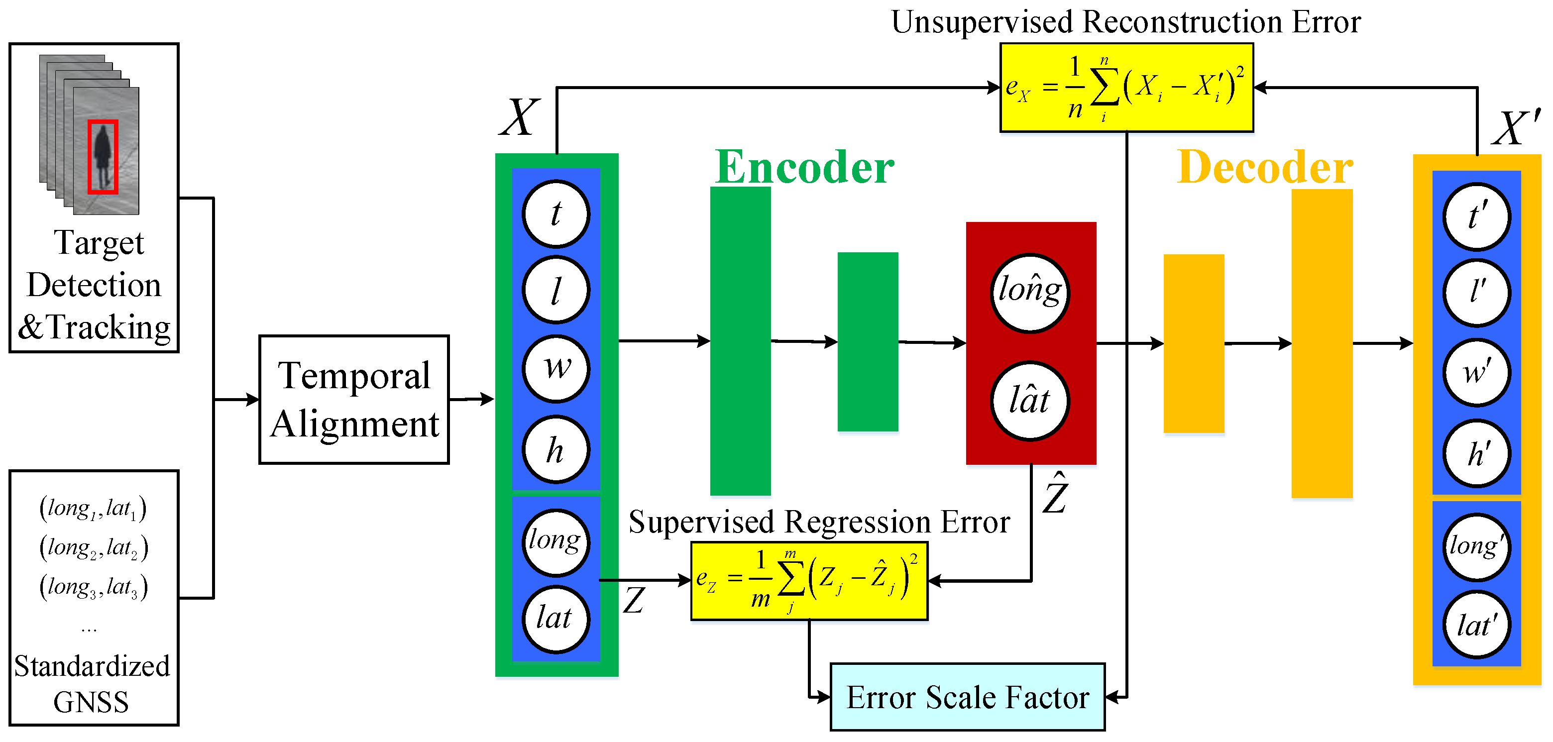
- We design a hybrid supervised and unsupervised auto-encoder fusion and regression framework for multi-sensor optimal position estimation. To the best of our knowledge, this is the first paper to optimize spatial positioning based on the fusion of image and GNSS using auto-encoder. We also mathematically prove that the proposed hybrid auto-encoder can yield optimal solution to the fusion and regression problem of multi-sensor position estimation;
- (3)
- Since our proposal is learning based, we make it possible that once the regression network is well trained offline with the assistance of GNSS, the camera itself can online automatically output the accurate geolocations of the targets in its view field. This function is significantly useful in some GNSS partially denied environments, where we first train a visual locator when GNSS is available, and then use it to predict the spatial positions of target when GNSS is not available;
- (4)
- We elaborately handcraft datasets which contain fixed camera images and GNSS in simulated and real-world scenes for the visual spatial positioning community. It is available at https://github.com/sculiang/image-spatial-localization (accessed on 23 April 2021).
2. Related Work
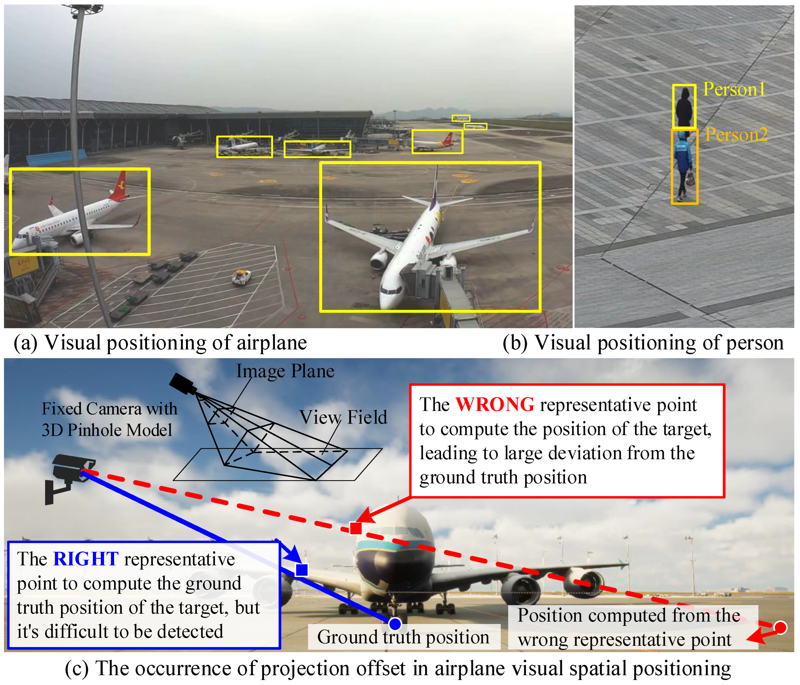
2.1. Image-Based Spatial Positioning
2.2. Multi-Sensor Fusion Based Spatial Positioning
3. Methodology
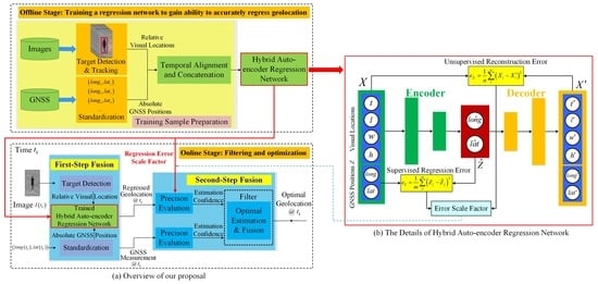
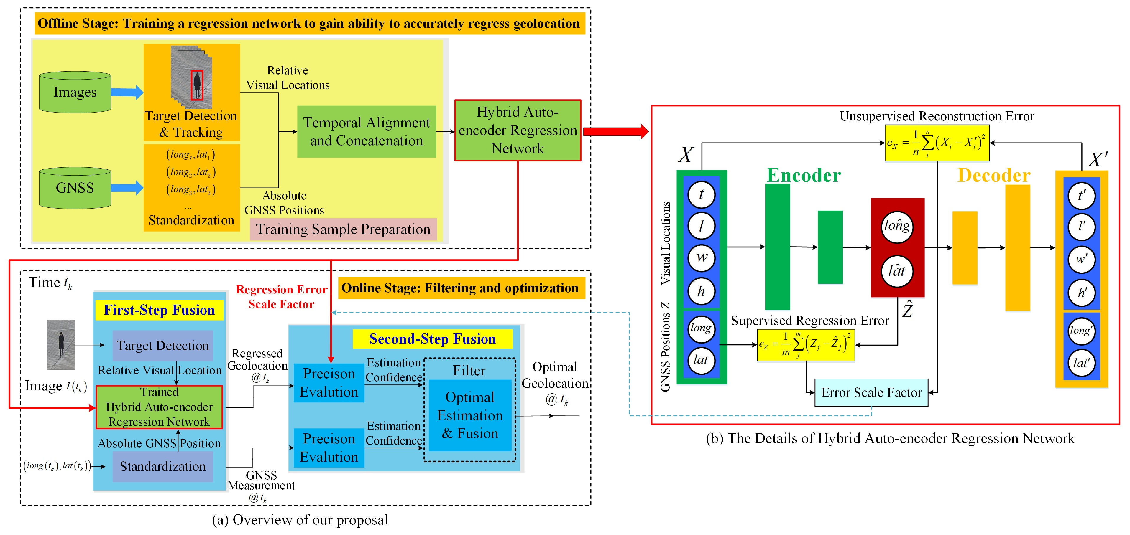
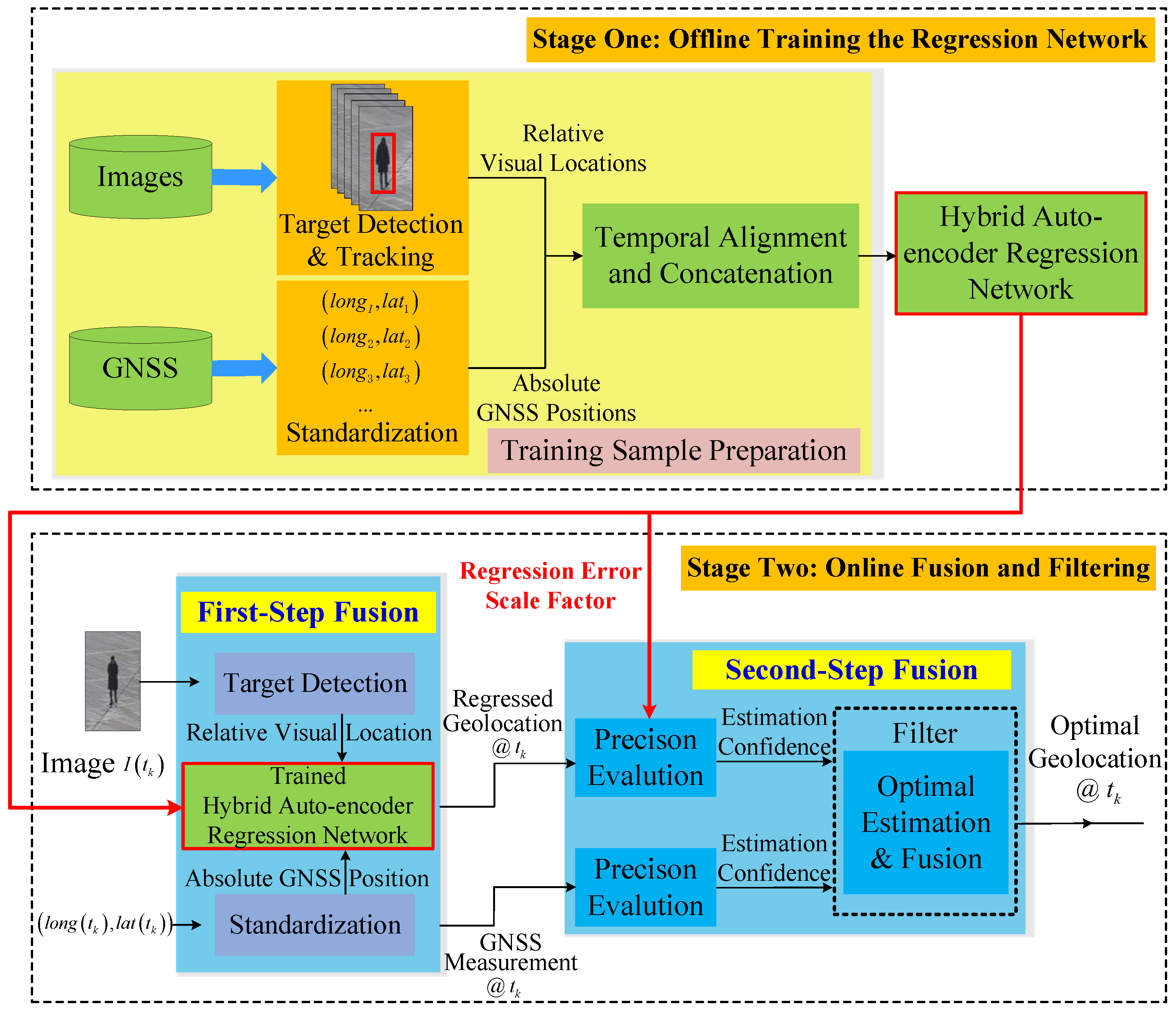
3.1. Stage One: Offline Training the Regression Network
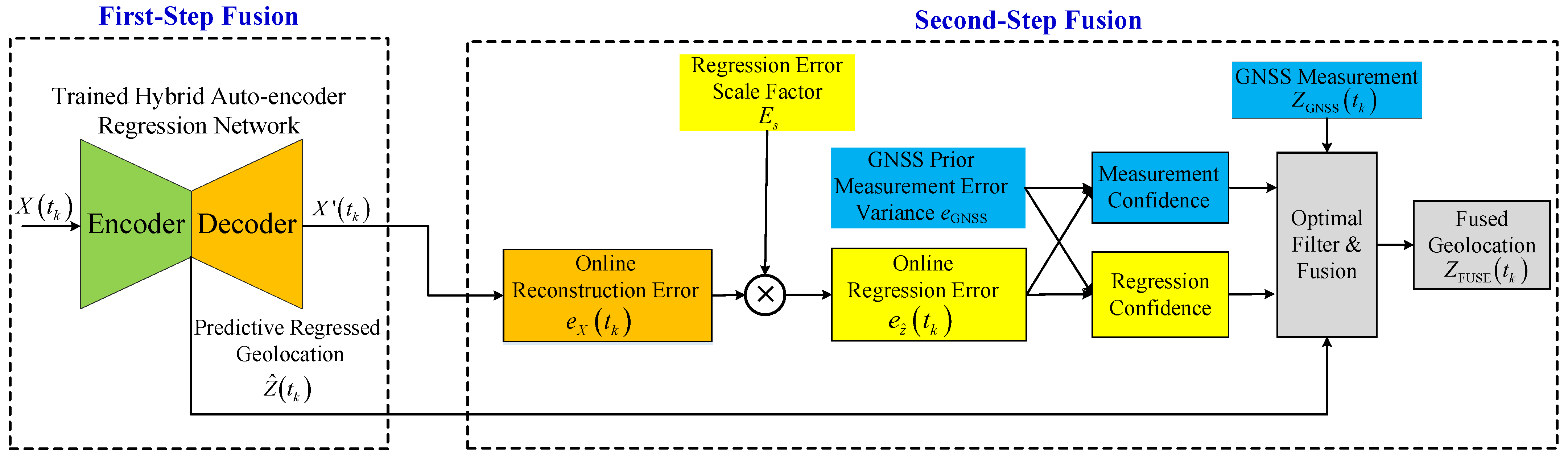
3.2. Stage Two: Online Fusion and Filtering
4. Experiments and Results
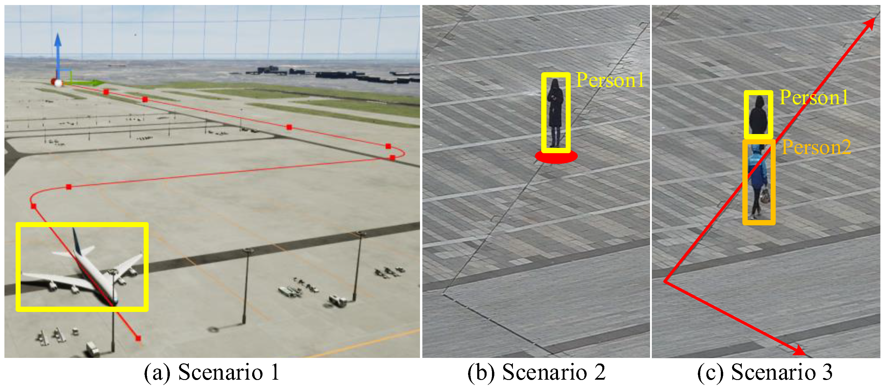
4.1. Experimental Setup
4.2. Experimental Results and Discussions
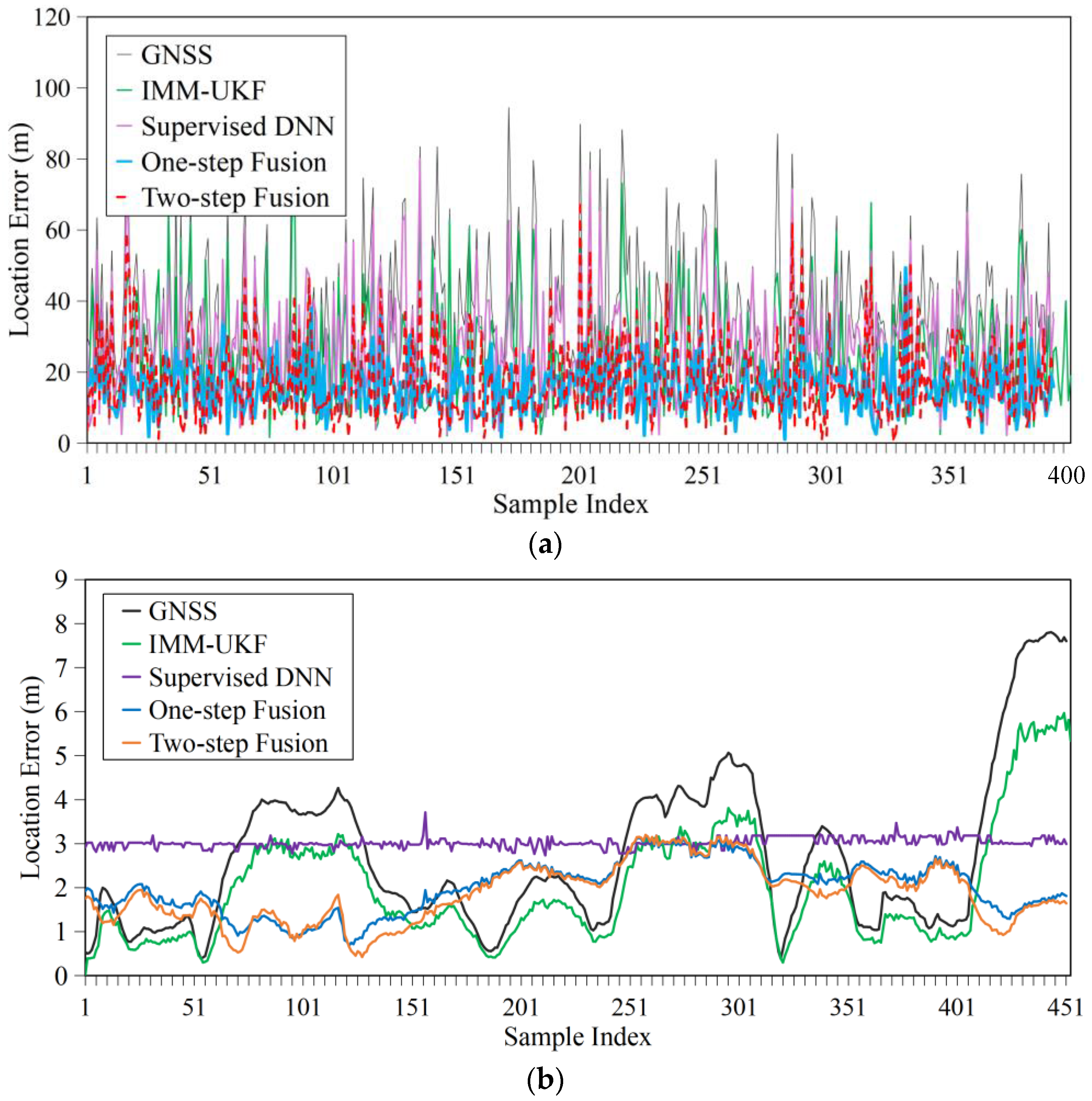
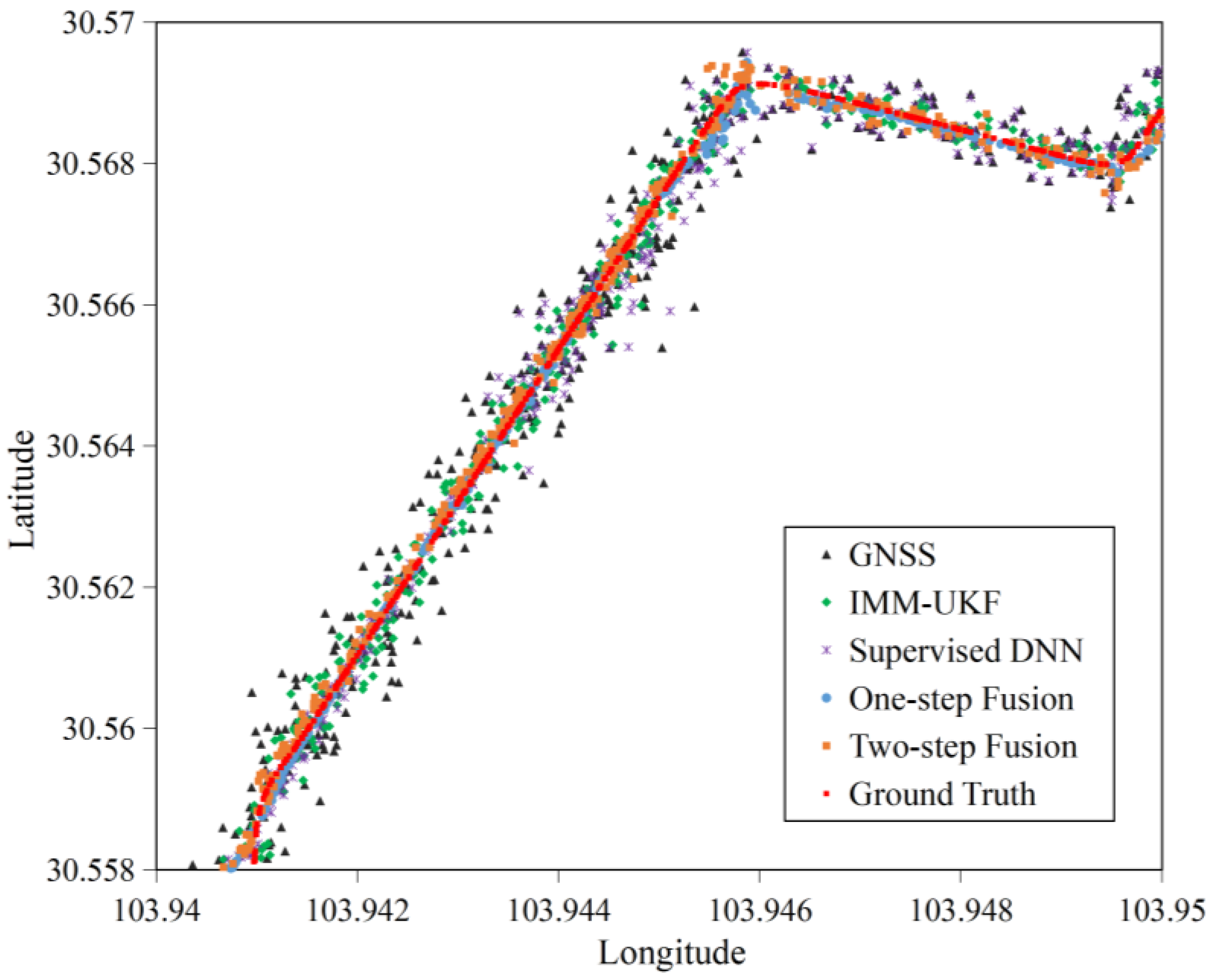
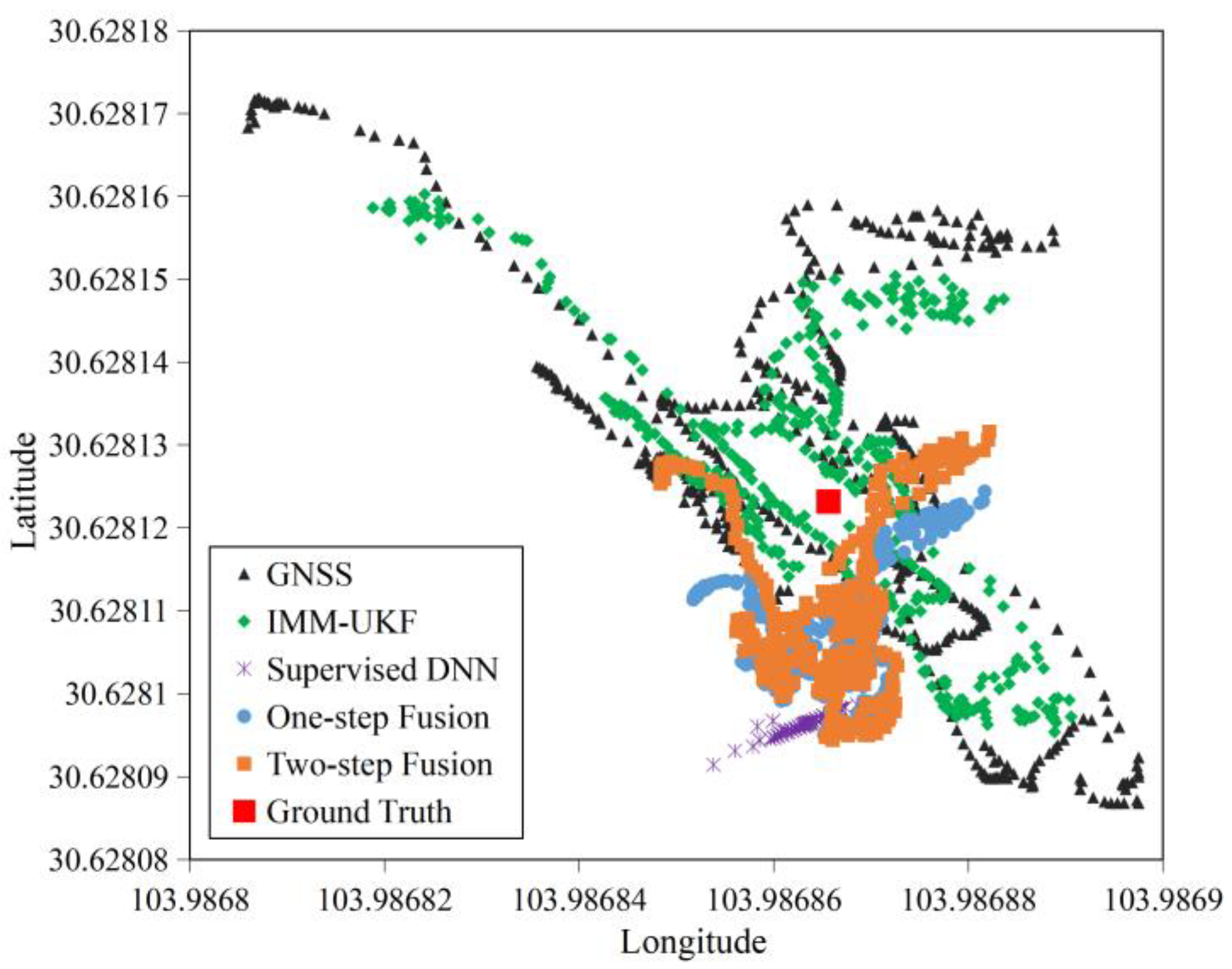
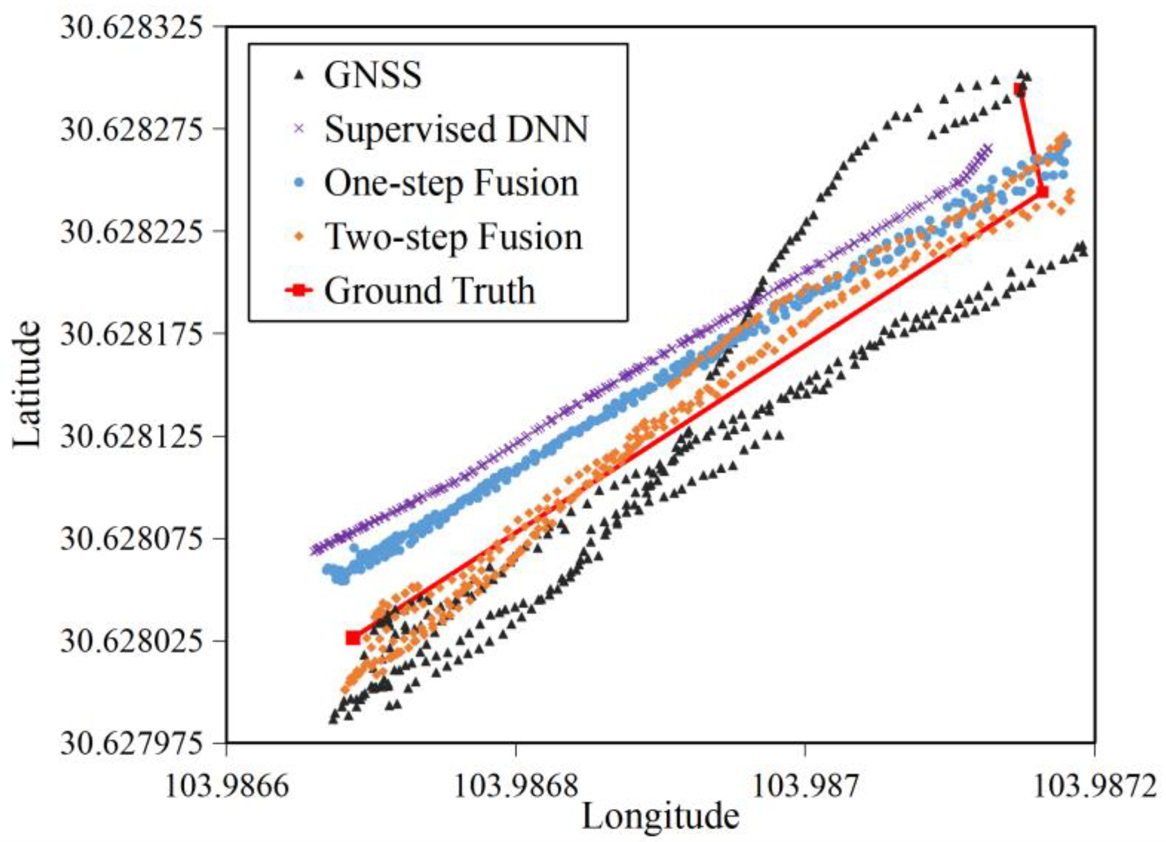
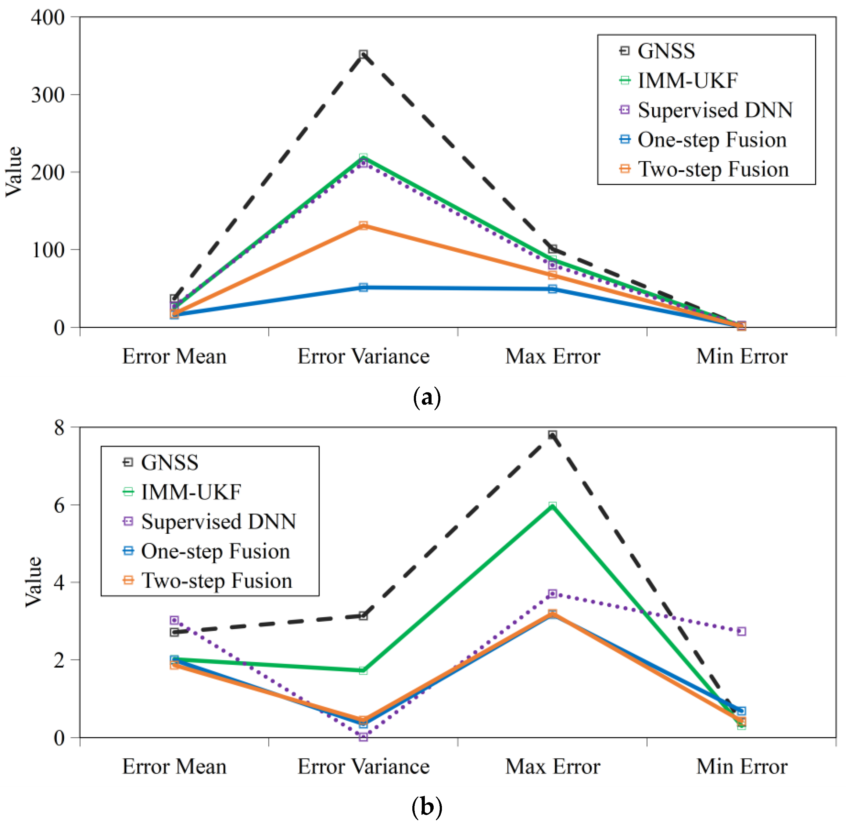
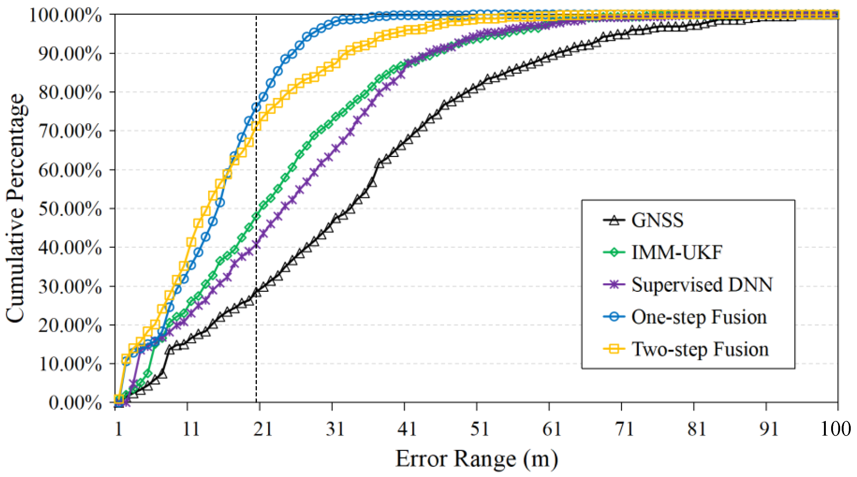
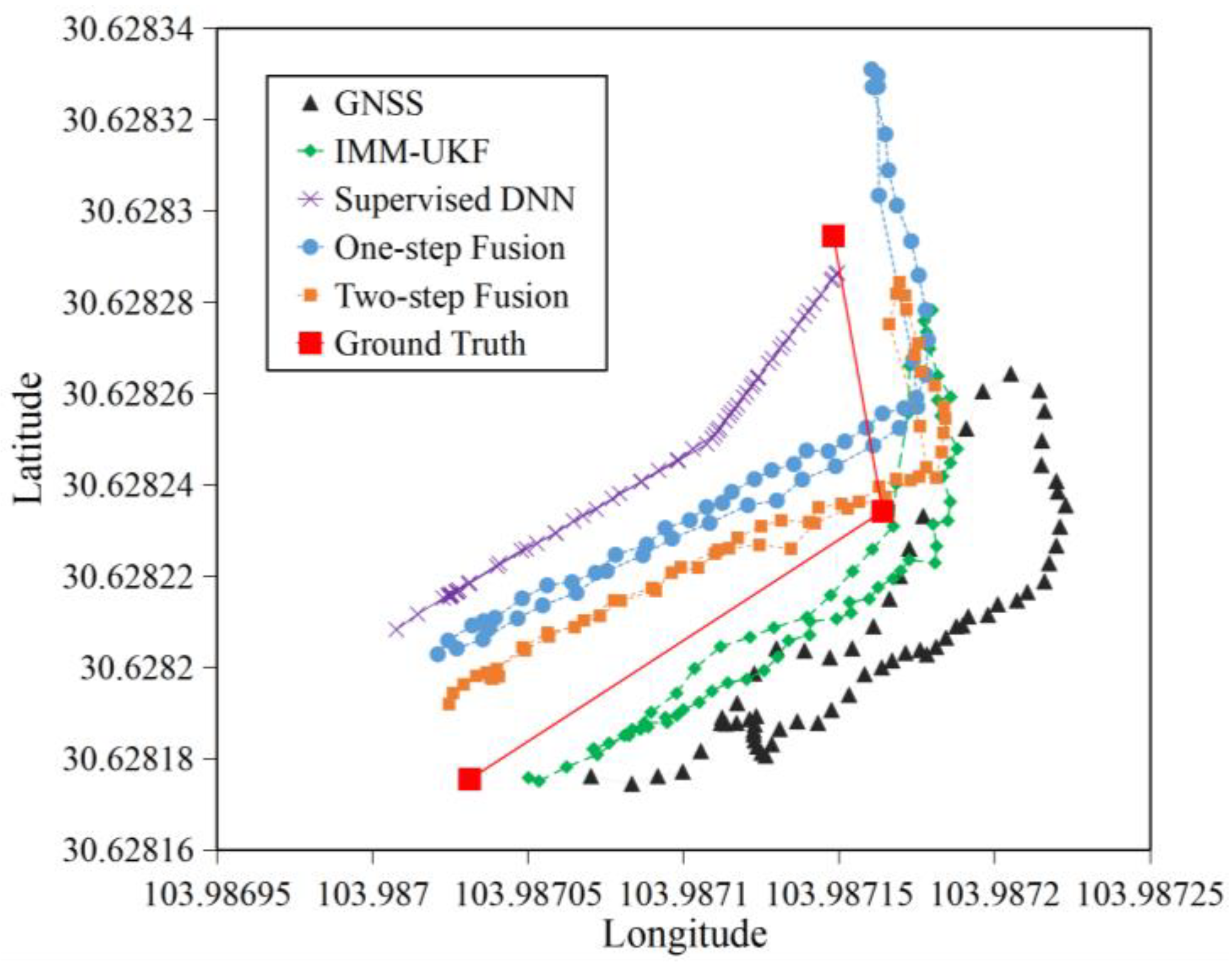
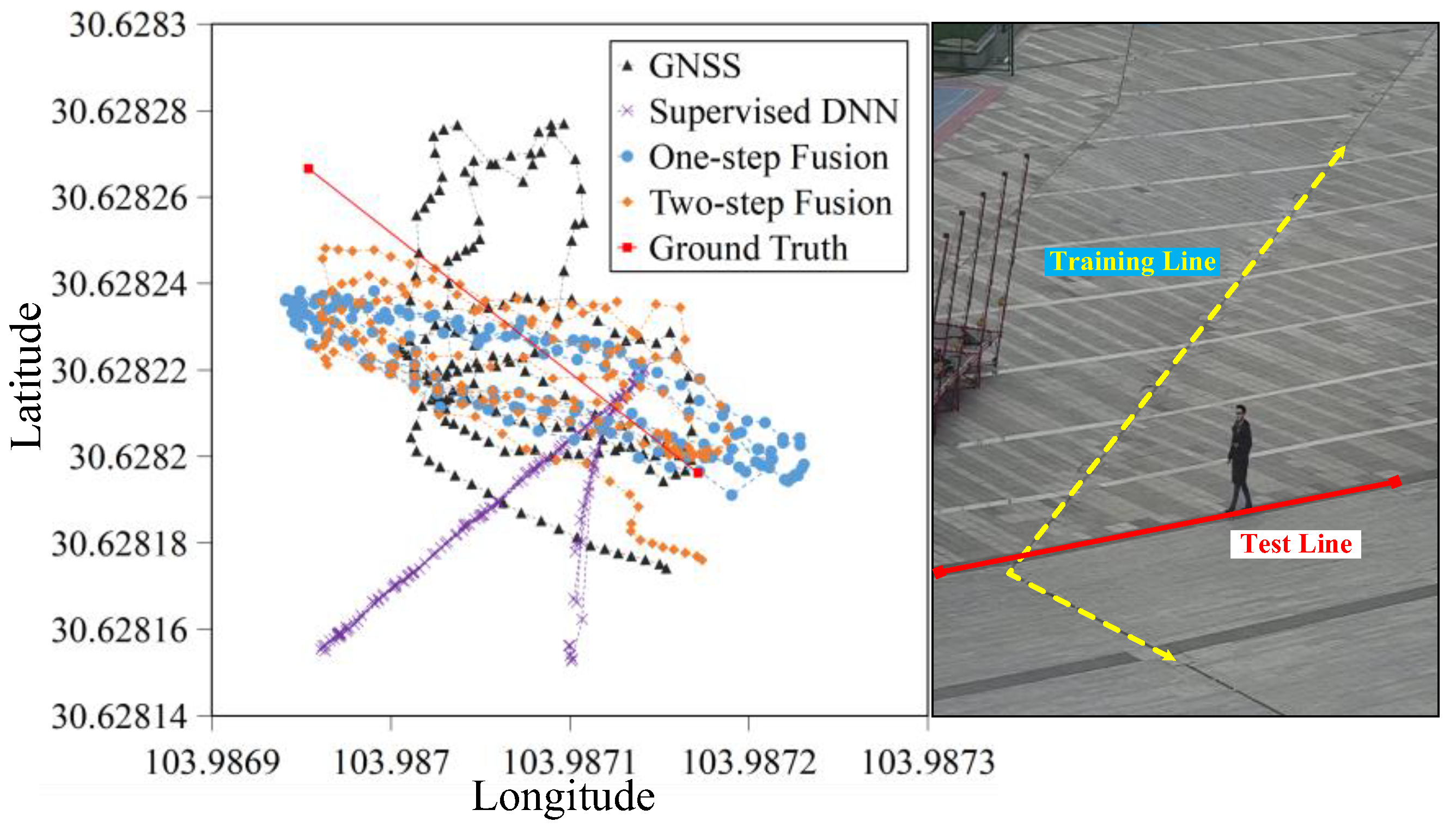
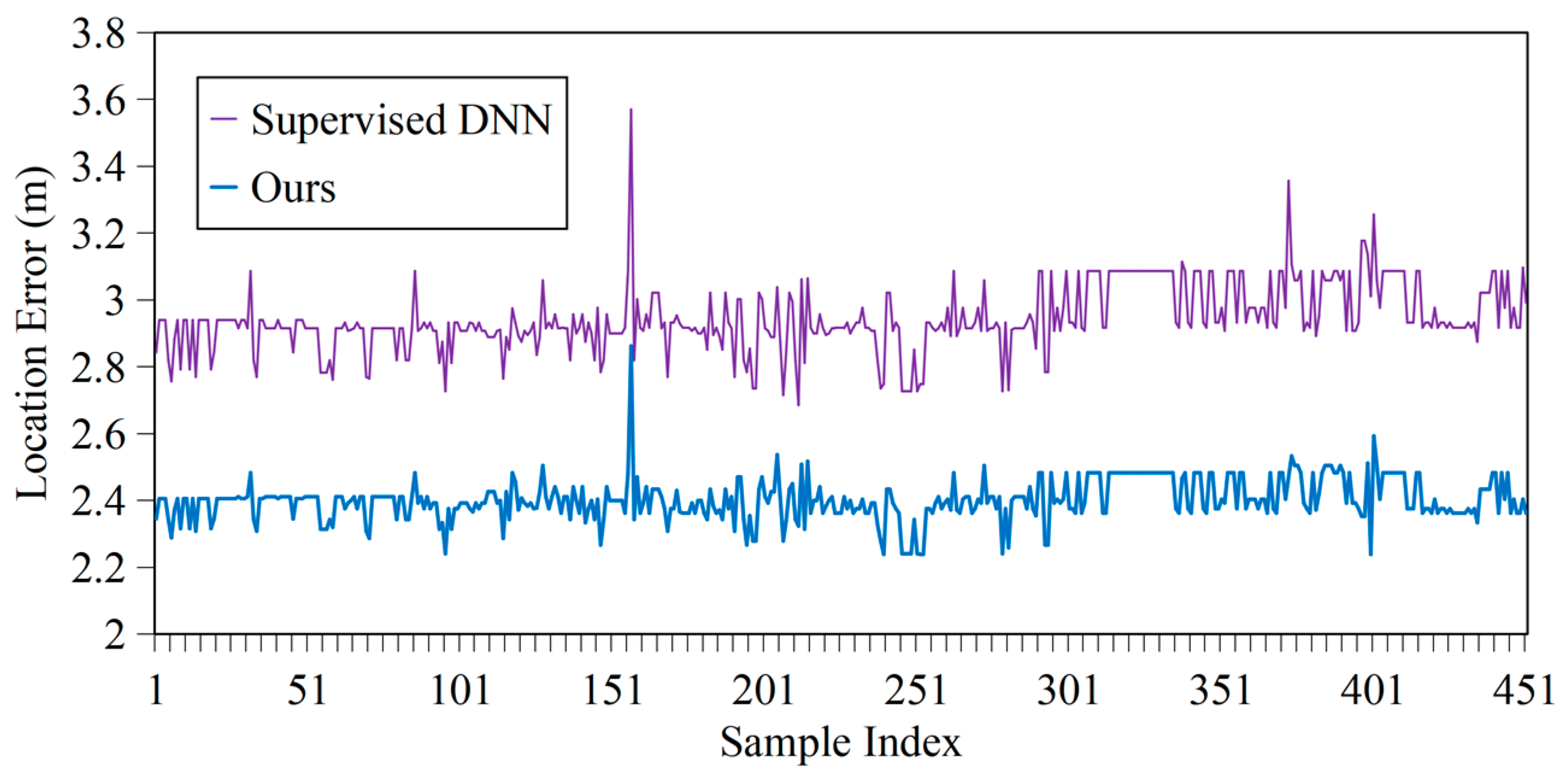
4.2.1. Accuracy
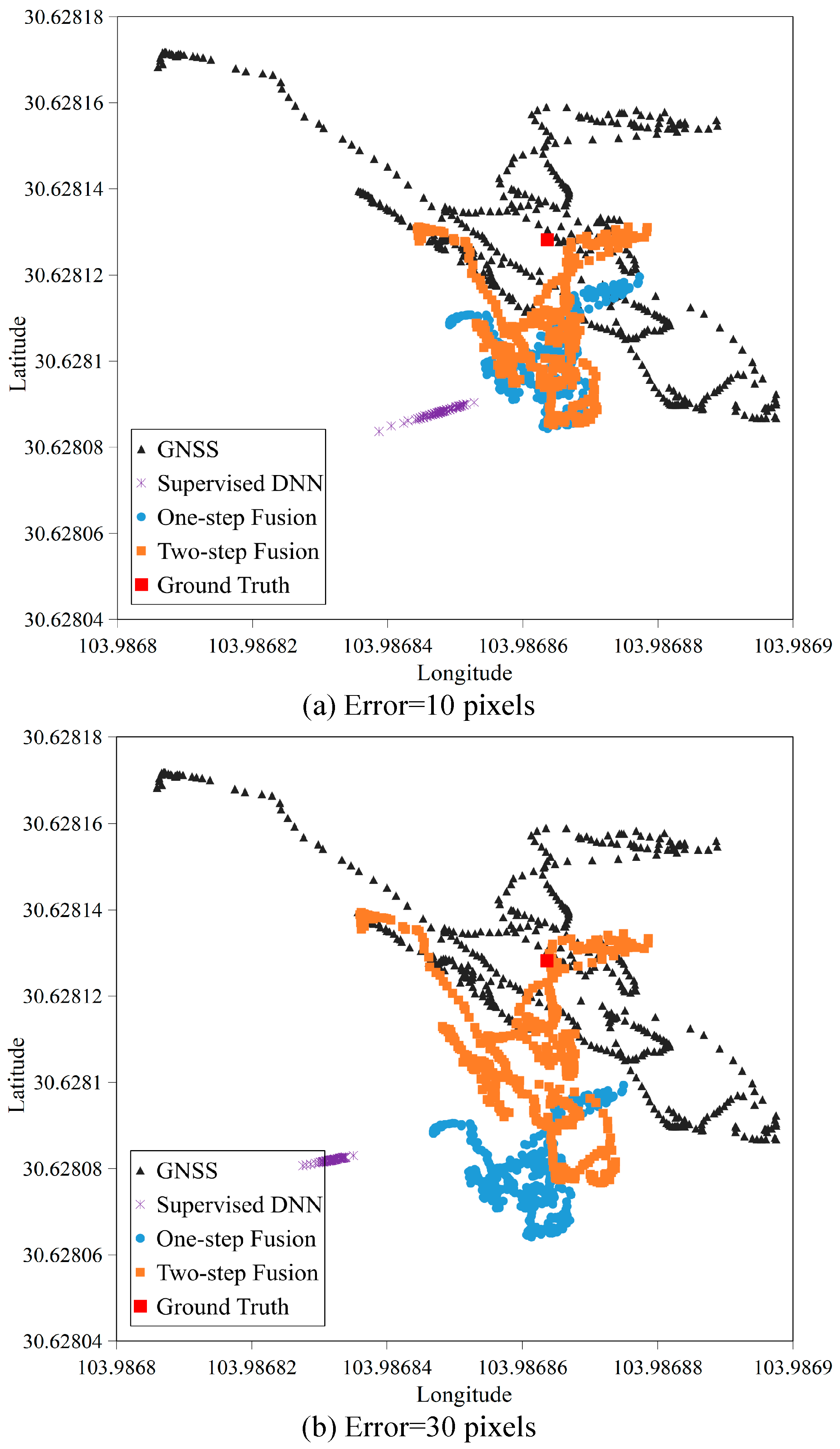
4.2.2. Robustness
4.2.3. Generalization
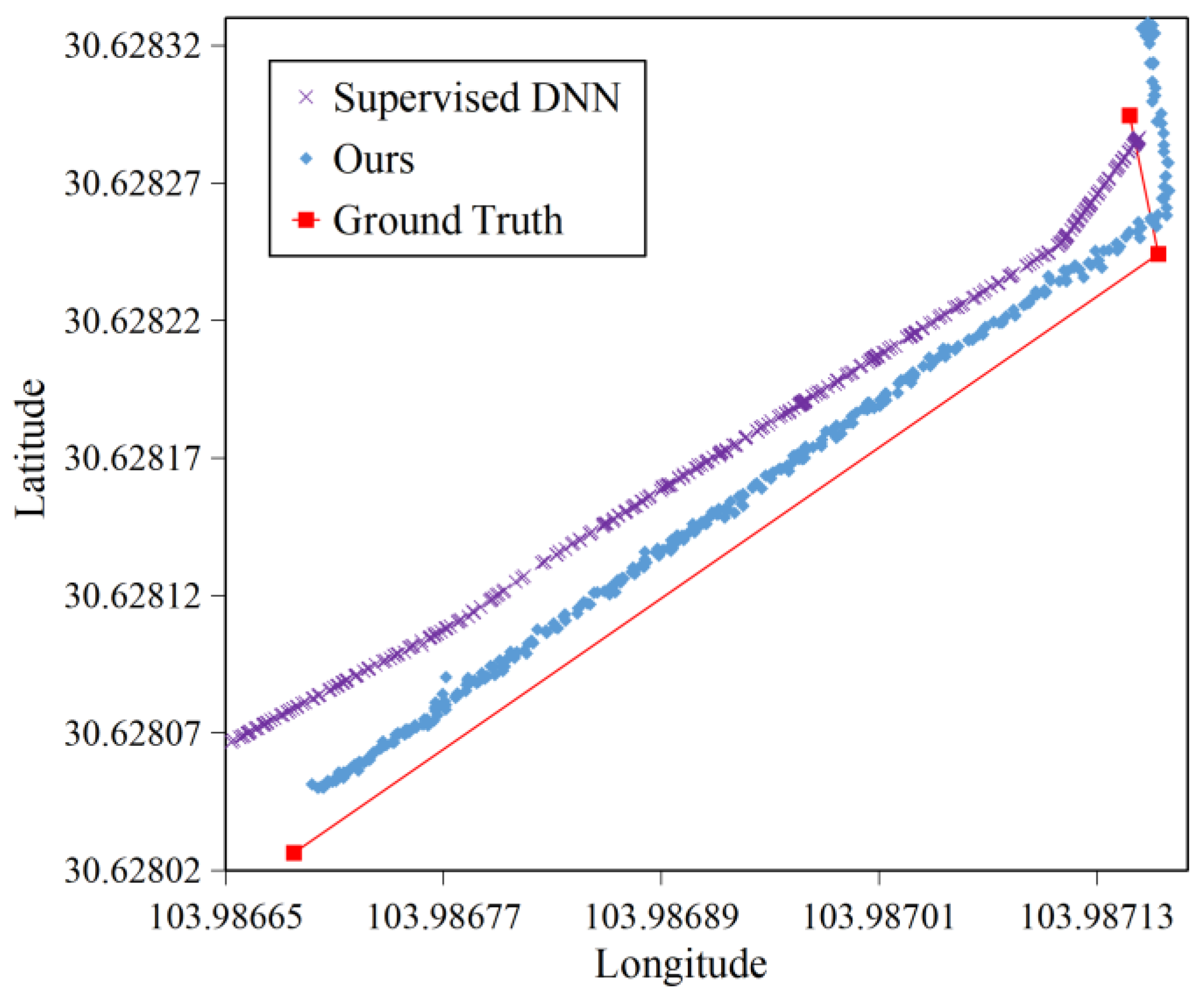
4.2.4. Performance in GNSS Denied Environments
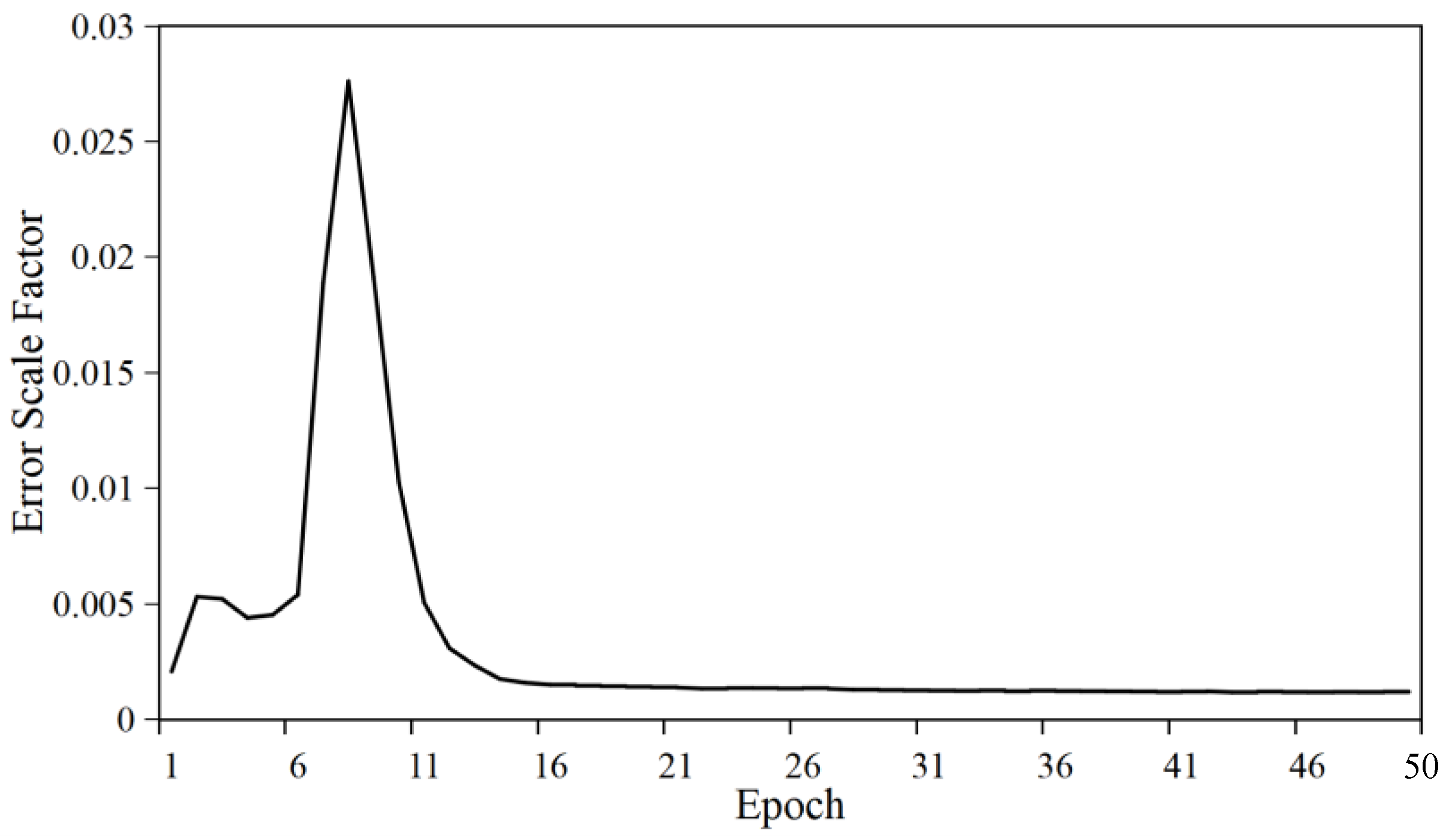
4.2.5. Convergence Analysis of Regression Error Scale Factor
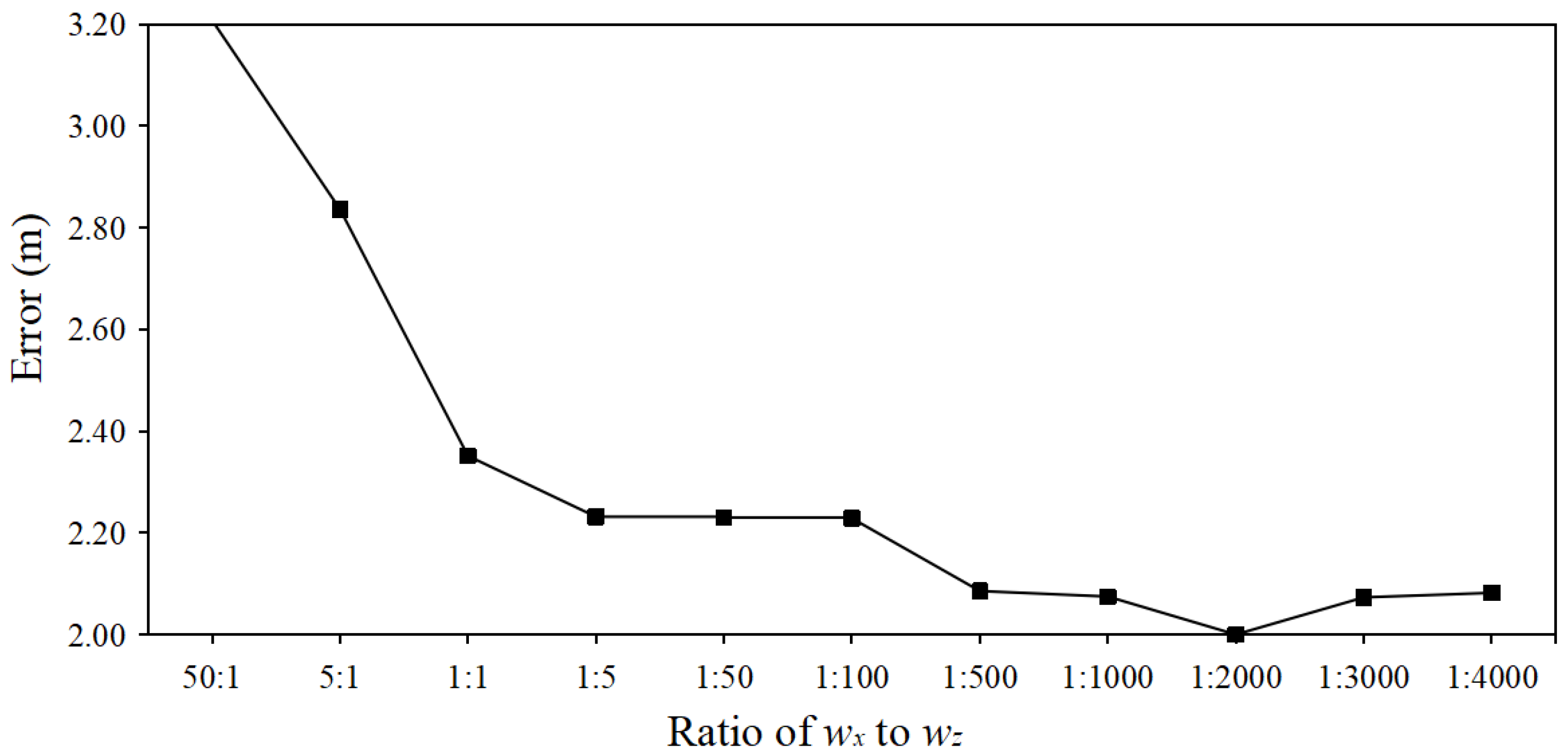
4.2.6. Comparative Analysis of Different and
5. Conclusions
Author Contributions
Funding
Conflicts of Interest
Appendix A. Mathematical Derivation that Our Hybrid Auto-Encoder Can Yield Optimal Solution to Our Regression Problem

References
- Zhang, Z. A flexible new technique for camera calibration. IEEE Trans. Pattern Anal. Mach. Intell. 2000, 22, 1330–1334. [Google Scholar] [CrossRef] [Green Version]
- Chuang, J.H.; Ho, C.H.; Umam, A.; Chen, H.Y.; Hwang, J.N.; Chen, T.A. Geometry- based camera calibration using closed-form solution of principal line. IEEE Trans. Image Processing 2021, 30, 2599–2610. [Google Scholar] [CrossRef] [PubMed]
- Chen, J.; Zhang, B.; Tang, X.; Li, G.; Zhou, X.; Hu, L.; Dou, X. On-Orbit Geometric Calibration and Accuracy Validation for Laser Footprint Cameras of GF-7 Satellite. Remote Sens. 2022, 14, 1408. [Google Scholar] [CrossRef]
- Xu, F.; Wang, H.; Liu, Z.; Chen, W. Adaptive Visual Servoing for an Underwater Soft Robot Considering Refraction Effects. IEEE Trans. Ind. Electron. 2020, 67, 10575–10586. [Google Scholar] [CrossRef]
- Gong, Z.; Tao, B.; Yang, H.; Yin, Z.; Ding, H. An Uncalibrated Visual Servo Method Based on Projective Homography. IEEE Trans. Autom. Sci. Eng. 2018, 15, 806–817. [Google Scholar] [CrossRef]
- Liang, X.; Wang, H.; Liu, Y.H.; You, B.; Liu, Z.; Jing, Z.; Chen, W. Fully Uncalibrated Image-Based Visual Servoing of 2DOFs Planar Manipulators with a Fixed Camera. IEEE Trans. Cybern. 2021, 1–14. [Google Scholar] [CrossRef]
- Abosekeen, A.; Iqbal, U.; Noureldin, A.; Korenberg, M.J. A Novel Multi-Level Integrated Navigation System for Challenging GNSS Environments. IEEE Trans. Intell. Transp. Syst. 2021, 22, 4838–4852. [Google Scholar] [CrossRef]
- Min, H.; Wu, X.; Cheng, C.; Zhao, X. Kinematic and dynamic vehicle model-assisted global positioning method for autonomous vehicles with low-cost GPS/camera/in-vehicle sensors. Sensors 2019, 19, 5430. [Google Scholar] [CrossRef] [Green Version]
- Chen, X.; Hu, W.; Zhang, L.; Shi, Z.; Li, M. Integration of low-cost GNSS and monocular cameras for simultaneous positioning and mapping. Sensors 2018, 18, 2193. [Google Scholar] [CrossRef] [Green Version]
- Baldoni, S.; Battisti, F.; Brizzi, M.; Neri, A. A hybrid position estimation framework based on GNSS and visual sensor fusion. In Proceedings of the 2020 IEEE/ION Position, Location and Navigation Symposium (PLANS), Portland, OR, USA, 20–23 April 2020; pp. 979–986. [Google Scholar]
- Bochkovskiy, A.; Wang, C.; Liao, H. YOLOv4: Optimal speed and accuracy of object detection. arXiv 2020, arXiv:2004.10934. [Google Scholar]
- Wu, Y.; Tang, F.; Li, H. Image-based camera positioning: An overview. Vis. Comput. Ind. Biomed. Art. 2018, 1, 8. [Google Scholar] [CrossRef] [PubMed] [Green Version]
- Huang, W.; Jiang, S.; Jiang, W. Camera Self-Calibration with GNSS Constrained Bundle Adjustment for Weakly Structured Long Corridor UAV Images. Remote Sens. 2021, 13, 4222. [Google Scholar] [CrossRef]
- Zhang, J.; Zhu, J.; Deng, H.; Chai, Z.; Ma, M.; Zhong, X. Multi-camera calibration method based on a multi-plane stereo target. Appl. Optics. 2019, 58, 9353–9359. [Google Scholar] [CrossRef] [PubMed]
- Nguyen, T.P.; Tran, T.H.P.; Jeon, J.W. MultiLevel Feature Pooling Network for Uncalibrated Stereo Rectification in Autonomous Vehicles. IEEE Trans. Ind. Inform. 2021, 68, 10281–10290. [Google Scholar] [CrossRef]
- Abdelaal, M.; Farag, R.M.; Saad, M.S.; Bahgat, A.; Emara, H.M.; El-Dessouki, A. Uncalibrated stereo vision with deep learning for 6-DOF pose estimation for a robot arm system. Robot. Auton. Syst. 2021, 145, 103847. [Google Scholar] [CrossRef]
- Wen, W.; Bai, X.; Kan, Y.C.; Hsu, L.T. Tightly coupled GNSS/INS integration via factor graph and aided by fish-eye camera. IEEE Trans. Veh. Technol. 2019, 68, 10651–10662. [Google Scholar] [CrossRef] [Green Version]
- Chang, L.; Niu, X.; Liu, T.; Tang, J.; Qian, C. GNSS/INS/LiDAR-SLAM integrated navigation system based on graph optimization. Remote Sens. 2019, 11, 1009. [Google Scholar] [CrossRef] [Green Version]
- Zheng, Z.; Li, X.; Sun, Z.; Song, X. A novel visual measurement framework for land vehicle positioning based on multimodule cascaded deep neural network. IEEE Trans. Ind. Inform. 2021, 17, 2347–2356. [Google Scholar] [CrossRef]
- Yuwen, X.; Chen, L.; Yan, F.; Zhang, H.; Tang, J.; Tian, B.; Ai, Y. Improved Vehicle LiDAR Calibration with Trajectory-Based Hand-Eye Method. IEEE Trans. Intell. Transp. Syst. 2022, 23, 215–224. [Google Scholar] [CrossRef]
- Xu, Q.; Li, X.; Chan, C.-Y. A Cost-Effective Vehicle Localization Solution Using an Interacting Multiple Model−Unscented Kalman Filters (IMM-UKF) Algorithm and Grey Neural Network. Sensors 2017, 17, 1431. [Google Scholar] [CrossRef]
- Chiang, K.W.; Le, D.T.; Duong, T.T.; Sun, R. The performance analysis of INS/GNSS/V-SLAM integration scheme using smartphone sensors for land vehicle navigation applications in gnss-challenging environments. Remote Sens. 2020, 12, 1732. [Google Scholar] [CrossRef]
- Yao, Y.; Xu, X.; Zhu, C.; Chan, C.Y. A hybrid fusion algorithm for GPS/INS integration during GPS outages. Measurement 2017, 103, 42–51. [Google Scholar] [CrossRef]
- Aslinezhad, M.; Malekijavan, A.; Abbasi, P. ANN-assisted robust GPS/INS information fusion to bridge GPS outage. EURASIP J. Wirel. Commun. Netw. 2020, 129. [Google Scholar] [CrossRef]
- Zhang, T.; Xu, X. A new method of seamless land navigation for GPS/INS integrated system. Measurement 2012, 45, 691–701. [Google Scholar] [CrossRef]
- Sun, S.; Sarukkai, R.; Kwok, J.; Shet, V. Accurate deep direct geo-positioning from ground imagery and phone-grade GPS. In Proceedings of the IEEE Conference on Computer Vision and Pattern Recognition Workshops, Salt Lake City, UT, USA, 18–22 June 2018; pp. 1129–11297. [Google Scholar]
- Liu, X.; Zhang, Z. A Vision-Based Target Detection, Tracking, and Positioning Algorithm for Unmanned Aerial Vehicle. Wirel. Commun. Mob. Comput. 2021, 2021, 5565589. [Google Scholar] [CrossRef]
- Zhang, H.; Hu, B.; Xu, S.; Chen, B.; Li, M.; Jiang, B. Feature fusion using stacked denoising auto-encoder and GBDT for Wi-Fi fingerprint-based indoor positioning. IEEE Access 2020, 8, 114741–114751. [Google Scholar] [CrossRef]
- Zhu, F.; Zhang, Y.; Su, X.; Li, H.; Guo, H. GNSS position estimation based on unscented Kalman filter. In Proceedings of the 2015 International Conference on Optoelectronics and Microelectronics (ICOM), Changchun, China, 16–18 July 2015; pp. 152–155. [Google Scholar]


| Scenarios | GNSS | IMM-UKF | Supervised DNN | One-Step Fusion | Two-Step Fusion |
|---|---|---|---|---|---|
| Scenario 1 | 36.95 | 25.42 | 27.32 | 15.95 | 17.67 |
| Scenario 2 | 2.72 | 2.02 | 3.03 | 2.00 | 1.87 |
| Location Error | Mean (m) | Variance (m2) | Maximum (m) |
|---|---|---|---|
| Supervised DNN | 3.02 | 0.01 | 3.57 |
| Our One-step Fusion | 2.40 | 0.004 | 2.86 |
Publisher’s Note: MDPI stays neutral with regard to jurisdictional claims in published maps and institutional affiliations. |
© 2022 by the authors. Licensee MDPI, Basel, Switzerland. This article is an open access article distributed under the terms and conditions of the Creative Commons Attribution (CC BY) license (https://creativecommons.org/licenses/by/4.0/).
Share and Cite
Liang, B.; Han, S.; Li, W.; Fu, D.; He, R.; Huang, G. Accurate Spatial Positioning of Target Based on the Fusion of Uncalibrated Image and GNSS. Remote Sens. 2022, 14, 3877. https://doi.org/10.3390/rs14163877
Liang B, Han S, Li W, Fu D, He R, Huang G. Accurate Spatial Positioning of Target Based on the Fusion of Uncalibrated Image and GNSS. Remote Sensing. 2022; 14(16):3877. https://doi.org/10.3390/rs14163877
Chicago/Turabian StyleLiang, Binbin, Songchen Han, Wei Li, Daoyong Fu, Ruliang He, and Guoxin Huang. 2022. "Accurate Spatial Positioning of Target Based on the Fusion of Uncalibrated Image and GNSS" Remote Sensing 14, no. 16: 3877. https://doi.org/10.3390/rs14163877
APA StyleLiang, B., Han, S., Li, W., Fu, D., He, R., & Huang, G. (2022). Accurate Spatial Positioning of Target Based on the Fusion of Uncalibrated Image and GNSS. Remote Sensing, 14(16), 3877. https://doi.org/10.3390/rs14163877