Article

A Spatial Downscaling Method for Remote Sensing Soil Moisture Based on Random Forest Considering Soil Moisture Memory and Mass Conservation

1
Southern Marine Science and Engineering Guangdong Laboratory (Zhuhai), Guangdong Province Key Laboratory for Climate Change and Natural Disaster Studies, School of Atmospheric Sciences, Sun Yat-sen University, Guangzhou 510275, China
2
College of Computer Science and Technology, Changchun Normal University, Changchun 130032, China
3
State Key Laboratory of Severe Weather, Chinese Academy of Meteorological Sciences, Beijing 100081, China
4
Guangdong Climate Center, Guangzhou 510275, China
*
Author to whom correspondence should be addressed.
Remote Sens. 2022, 14(16), 3858; https://doi.org/10.3390/rs14163858
Submission received: 3 July 2022 / Revised: 3 August 2022 / Accepted: 5 August 2022 / Published: 9 August 2022
(This article belongs to the Section AI Remote Sensing)

Abstract

:
Remote sensing soil moisture (SM) has been widely used in various earth science studies and applications, but their low resolution limits their usage and downscaling of them is needed. In this study, we proposed a spatial downscaling method for SM based on random forest considering soil moisture memory and mass conservation to improve downscaling performance. The lagged SM was added as a predictor to represent soil moisture memory, in addition to the regular predictors in previous downscaling studies. The Soil Moisture Active Passive (SMAP) SM data of the Pearl River Basin were used to test our downscaling method. The results show that the downscaling model obtained good performance on the test set (R2 = 0.848, ubRMSE = 0.034 m3/m3 and Bias = 0.008 m3/m3). The spatial and temporal performance of the RF downscaling model can be improved by adding lagged SM variables. Downscaled data obtained can retain the information of the original SMAP SM data well and show more spatial details, and mass conservation correction is considered to be useful to eliminate systematic bias of the downscaling model. Downscaled SM achieved acceptable performance in in situ validation, though it was inevitably limited by the performance of the original SMAP data. The proposed downscaling method can serve as a powerful tool for the development of high-resolution SM information.

Graphical Abstract

1. Introduction

Soil moisture (SM) is a key variable in the Earth system, which controls the exchange of water and energy fluxes between land surface and atmosphere [1]; it plays an important role in the circulation of water and energy of the Earth system [2,3]. SM has a wide range of applications in drought monitoring [4], water resources management [5,6], weather forecasting [2,7,8], geological disaster detection [9] and other aspects. Therefore, it is of great significance to obtain accurate temporal and spatial distribution of SM.
However, due to the common impact of topography, soil, landcover and meteorological forcing [10,11], SM has high spatial heterogeneity, and it is still challenging to obtain high precision SM information. The traditional ground-based measurements of SM such as gravimetric methods [12,13], neutron scattering [14], time domain reflectometry [13,15] can obtain relatively reliable SM at different depths, but it is still not easy to obtain spatially continuous distribution of SM at different spatial scales through ground-based measurements due to their poor spatial representativeness, especially for areas with sparse sites.
With the development of remote sensing techniques, SM from regional to global scales can be obtained by different satellites, through making use of the connection between the electromagnetic radiation and SM. Many SM products from different microwave sensors have been widely used, such as Advanced Microwave Scanning Radiometer–EOS (AMSR-E) [16], the Soil Moisture and Ocean Salinity (SMOS) [17,18], and the Soil Moisture Active Passive (SMAP) mission [17].
However, as most of SM products mentioned above have a relatively coarse spatial resolution (around tens of kilometers), which limits their applications in hydrological and agricultural studies; it is necessary to downscale SM products to meet resolution requirements in the practical applications. In order to obtain SM spatial information with finer resolution, several downscaling methods have been proposed to downscale SM, such as the regression fitting approach [19,20,21], disaggregation based on physical and theoretical scale change (DISPATCH) [22,23] and machine learning approach [24,25].
The statistics-based and physics-based downscaling method mentioned above is mainly based on the idea of establishing a statistical correlation or a physical-based model between coarse-scale SM and fine-scale auxiliary variables [26]. Among the methods, the so-called polynomial-fitting method based on the “universal triangle” space between LST and vegetation index was widely applied in many studies [9,19,20,21,27,28]. This method expressed the high-resolution SM as a polynomial function of LST, vegetation index, and surface albedo derived from optical/thermal data [26]. However, most existing downscaling methods, especially the polynomial-fitting method, cannot describe the complicated relationship between the SM and auxiliary variables due to their linear fitting assumption [29,30].
Inspired by the great ability to model the nonlinear relationship between the auxiliary variables and prediction variables, the machine learning downscaling method has been proposed to obtain remote sensing products with finer resolution, not only SM products [24,25,31,32,33,34,35,36,37]. Among these machine learning downscaling methods, random forest (RF) was a popular and convenient machine learning model to be used to downscale SM products. Liu et al. (2020) compared the SM downscaling performance of six machine learning models and found that RF is the best model in the comparison [37]. Among the previous machine learning downscaling studies, auxiliary variables which are considered to be closely related to SM, including LST, vegetation index, albedo derived from optical/thermal data and topographical parameters are applied in different machine learning models. These machine learning methods are data-driven methods, similar to the regression fitting approach which depends on the relationship between auxiliary variables derived from optical/thermal satellites and passive remote sensing SM, though they have better performance. Therefore, the downscaling performance of these machine methods may also be influenced by the availability of optical/thermal data, such as other regression fitting downscaling approaches [38,39]. In addition, the methods depending on optical/thermal data rely on a strong atmospheric evaporative demand and are more adapted to arid and semiarid areas because LST is linked to SM in the case of nonenergy limited conditions [26].
The selection of the auxiliary variables of the machine learning downscaling methods mentioned above mainly focused on the variables with finer resolutions, and few studies viewed lagged SM (i.e., SM at previous time steps) as an important spatial downscaling feature. As the indicator of SM memory [40], lagged SM is often applied in the study of SM time series prediction [41,42], and it is considered as an important predicting variable in machine learning prediction models [43,44]. Therefore, adding lagged SM in machine learning downscaling methods may improve the representation of SM temporal characteristics and reduce the dependence on the availability of optical/thermal data. At the same time, the output data of these machine learning downscaling methods may have systematic errors that do not conform to the law of mass conservation, because these machine downscaling methods are statistic-based. Thus, downscaled data may be underestimated for high values and overestimated for low values.
In our study, we intended to downscale SMAP SM in the area of the Pearl River Basin (PRB) and improved the machine learning downscaling method by adding lagged SM variables as a predictor and introducing the correction of mass conservation to the downscaled SM. The objectives of our study were as follows: (1) to downscale SMAP SM in Pearl PRB through constructing a nonlinear relationship between SM and various predictors by random forest; (2) to explore and discuss the influence of the lagged SM values and correction of mass conservation on downscaling results; (3) to validate the performance of the downscaling model by in-situ data.
The arrangements of our paper are as follows. In Section 2, we introduce the study area, data and method. In Section 3 and Section 4, the result of the downscaling methods is shown and discussed. In Section 5, conclusions are presented.

2. Materials and Methodology

2.1. Study Area

The Pearl River Basin (PRB) is one of the three major basins in China, with an area of about 442,000 km2 [45]. Located in the subtropical monsoon climate zone, the PRB has an annual average temperature ranging from 14 °C to 22 °C. The annual average precipitation is between 1200 mm and 2200 mm, with uneven distribution in space and time. The precipitation is mainly concentrated from April to September each year, which accounts for 72% to 88% of the total annual precipitation [46]. The altitude of the basin becomes lower from the northwest to the southeast (Figure 1). The main vegetation cover of the basin is evergreen broad-leaved forest (65.3%), and agricultural land accounts for 18.1% of the total area (Figure 2). The flat areas in the downstream PRB have shown urban clusters with rapid social and economic development in recent decades. Therefore, high-precision soil moisture data is of great significance for land surface hydrology research and water resources management in the PRB.

2.2. Datasets

In this study, we downscaled the SMAP soil moisture by using multiply covariates (auxiliary variables) including MODIS, ERA5-Land, in situ soil moisture, soil properties and topographic data (Table 1). This section describes these data sets.

2.2.1. SMAP Soil Moisture

SMAP (Soil Moisture Active and Passive) satellite is one of the earth observation satellites of the United States, which was launched on 31 January 2015 [47]. Though SMAP originally planned to use L-band radar and radiometers to measure surface SM at different resolutions at global scale, only passive radiometers work after 31 January 2015 when radar sensors failed to work on. SMAP satellite is in near-polar orbit and passes over the observation area at 06:00 (descend) and 18:00 (ascend) local time. Some studies have shown that SMAP passive remote sensing products have reached the accuracy requirements of the satellite launch mission [48,49]. Therefore, SMAP passive remote sensing products play an important role in global soil moisture detection.
In our work, we used SMAP Level-3 (L3) passive SM product with a spatial resolution of 36 km as our downscaling target. Zhao et al. (2018) have found that data from ascending and descending half-orbits have little influence to the downscaling process [50]. Therefore, in order to obtain as much training samples for RF model as possible and improve the representativeness of the data, we used the average of the SMAP L3 SM (after quality control) of ascending and descending half-orbits to obtain the daily SMAP L3 SM for downscaling.

2.2.2. CMA In Situ Soil Moisture

The in situ SM data is obtained from the China Meteorological Administration (CMA), which provides SM measurement data from 10-cm depth to 100-cm depth. We selected the SM data at the 10-cm depth from the 120 stations located in our study region to validate our downscaled SM. Due to some measurement sensor may occur to break down, we deleted some constant values, abnormally high and low values in in situ data for quality control following the method of Dorigo et al. (2013) [51].

2.2.3. MODIS Data

As mentioned in Section 1, surface variables such as land surface temperature (LST), vegetation index and albedo have been widely used to build the relationship between auxiliary variables and SM. Therefore, we used the MODIS (moderate-resolution imaging spectroradiometer) products for these variables. The MODIS products used in our paper include 1-km resolution daily LST (MOD11A1 from Terra satellites and MYD11A1 from Aqua satellite) [52], 1-km resolution 16-day Normalized Difference Vegetation Index (NDVI) and Enhanced Vegetation Index (EVI) (MOD13A2 from Terra satellite and MYD12A2 from Aqua satellite) [53], 500-m resolution 16-day albedo (MCD43A3) [54].
Similar to SMAP L3 SM, the mean values of MODIS datasets were calculated to obtain as many training samples as possible. The temporal resolution of 16-day was interpolated to 1-day by the linear interpolation method. The actual albedo was calculated by empirical equations proposed by [55]. The equations are as follows:
a = absa × (1 − r) + awsa × r
r = 0.122 + 0.85 × exp (−4.8 × cosθ)
absa and awsa are Black-Sky Albedo and White-Sky Albedo from MODIS respectively, and θ is the solar zenith angle at noon. We found that the near-infrared band albedo of the study area has too many missing values, so we abandoned this variable in our model.

2.2.4. ERA5-Land Data

The precipitation data in our work come from ERA5-Land datasets. ERA5 datasets is the fifth-generation reanalysis dataset of global climate from the European Centre for Medium-Range Weather Forecasts (ECMWF). ERA5-Land is an enhanced version of ERA5 land component, forced by meteorological fields from ERA5 [56,57]. This dataset provides hourly data of land surface variables, such as precipitation, soil moisture, and radiation, with a spatial resolution of 0.1°, and plays an important role in flood or drought monitoring.

2.2.5. Chinese Soil Properties Dataset

The soil properties variables used in our work are the proportion of sand, silt and clay. These data come from the Chinese soil properties dataset used in The Common Land Model (CoLM) [58]. This dataset was developed from the Soil Map of China (1:1,000,000) and 8979 soil profiles, and it provides physical and chemical attributes with a spatial resolution of 30 arc-second (about 1 km), which has higher quality than the HWSD (Harmonized World Soil Database) because it used more soil profiles, a soil map with higher resolution, and more reasonable study method and quality control [59].

2.2.6. Topographic Data

Topographic variables can influence the spatial distribution of SM at different scale [60] and have been applied in many downscaling studies [61,62,63,64]. We used the altitude variable as the topographic variable of the downscaling model. The altitude data come from the Shuttle Radar Topography Mission (SRTM) [65]. The topographic data can be download from http://earthexplorer.usgs.gov/ (accessed on 6 April 2022)

2.3. Methods

2.3.1. Random Forest

Random forest (RF) is a popular machine learning method widely used in many studies [66]. This method has great fitting ability for classification and regression problems. RF builds some decision trees in the training process, and it outputs the mean values of prediction from these decision trees as the prediction of the whole model. RF splits the input feature space into many decision trees; hence, it is called forest. The training samples input in each decision tree is generated by the bootstrap sample method, which can ensure that the RF model includes different kinds of decision trees generated by different training subset. Due to the bootstrap sample method, not all of the training samples are used to train the model. Usually, two thirds of the training samples are selected to build trees, and the rest of the samples will be used to validate each tree. This concept is known as out-of-bag samples to estimate the model generalization errors. RF reduces generalization errors by assembling the predictions generated from each tree, which makes it stable and difficult to overfit. The RF model used in our paper was established using sklearn package in python. In the aspect of super parameter setting, in order to prevent the model from overfitting and ensure the training efficiency, the number of trees (n_estimators) was set to 1000, and other super parameters were set by grid search method (min_samples_split: 4; max_depth parameters: 28), though it cannot improve models significantly compared to the default settings.

2.3.2. Downscaling Process

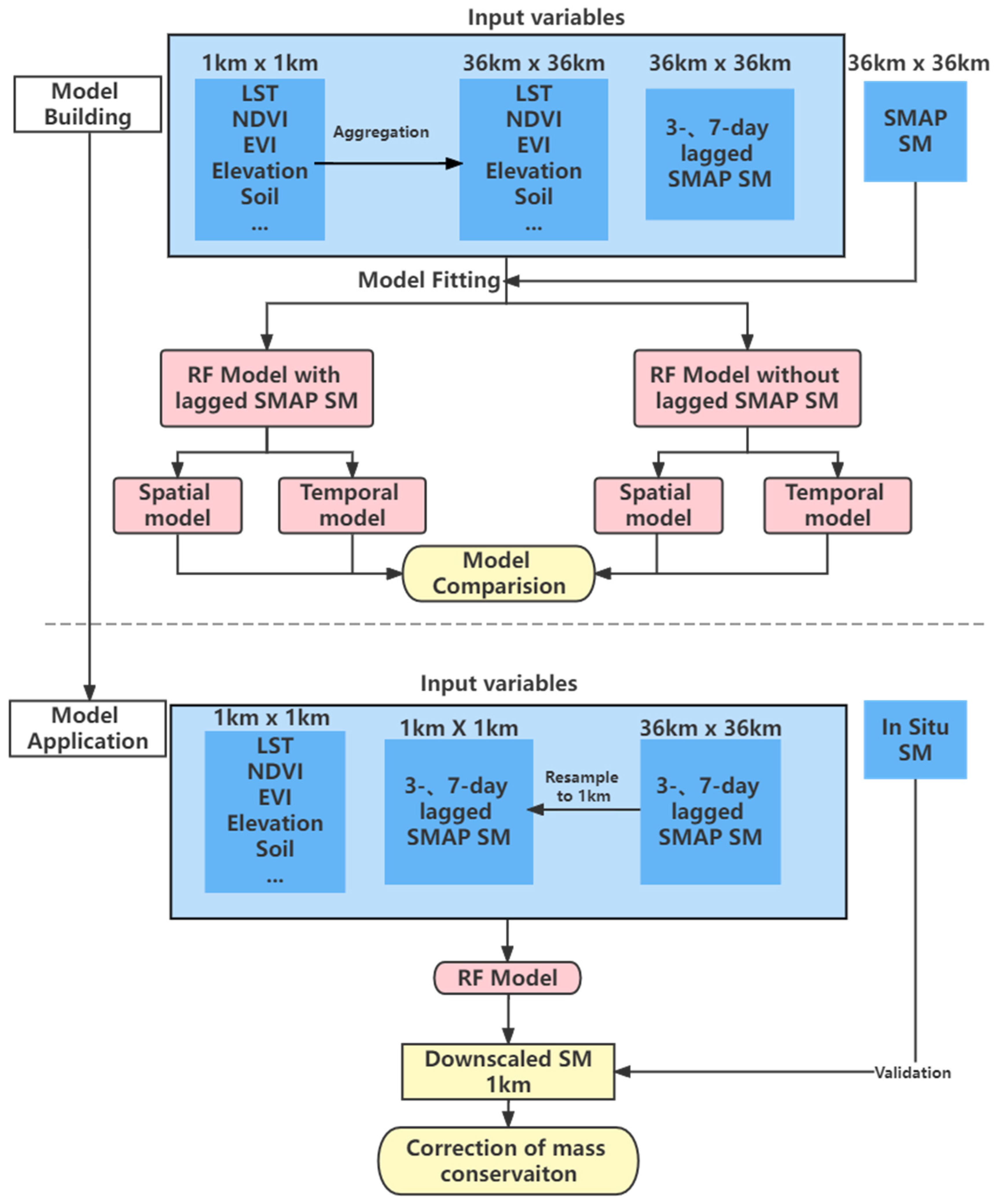
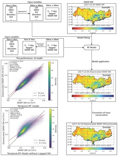
The flow chart of our experiment is shown in Figure 3. The upper part of the figure is about the establishment of the downscaling model and the rest part of the figure is about the application and validation of the downscaling model. The whole process of our experiment is as follows:
(1)
Firstly, we aggregated the variable with finer resolution to 36 km, which is consistent with SMAP SM, by the mean of arithmetic average [67], because the training process is on the 36-km grids of the SMAP SM. In order to ensure the representativeness of the data, if the invalid proportion of some variables was more than 50% of the corresponding 36-km grid in the aggregation, we would view the output of this aggregation as invalid value. Otherwise, the corresponding grid is not used. This is inevitable for the reason of cloud cover to optical/thermal remote sensing data and scanning gap.
(2)
Then, in order to explore if the lagged SM can improve the downscaling model, we trained a downscaling model with lagged SM and another one without lagged SM for comparison. The three-day and seven-day lagged SM were selected according our primary experiments using different days of lagged SM.
(3)
We adopted two strategies to split the train set and test set to explore the temporal and spatial performance of the downscaling model. In temporal splitting strategy, we randomly selected half of the study date as train set, and the rest as test set. The temporal splitting strategy means that all samples of the whole study area on a day are either in the train set or in the test set. In spatial splitting strategy, we randomly selected half of the 36-km grids of the study area as train set, and the rest as test set. The spatial splitting strategy means that all samples of the whole time series on a 36-km grid are either in the train set or in the test set. Through temporal and spatial splitting strategies, we can obtain the performance of downscaling model on temporal test set and spatial test set.
(4)
Auxiliary data processed to the resolution of 1-km were input to the downscaling model to obtain the downscaled SMAP SM. Before inputting, we resampled the 36-km lagged SM to 1 km by means of simple bilinear interpolation. We validated the downscaled SM with in situ data and compared the downscaled SM with the original SMAP SM. Finally, we made correction of mass conservation to the downscaled SM, which makes the mean values of downscaled SM (1296 grids) in an original 36-km grid the same as the values of the original SMAP SM.

2.3.3. Evaluation Method

In order to evaluate the performance of the downscaling model, we used five statistical metrics to evaluate the model. The metrics include determination coefficient (R2), Pearson correlation coefficient (r), root mean square error (RMSE), unbiased RMSE (ubRMSE), and bias. The calculation equations of these metrics are as follows:
R 2 = 1 i = 1 n ( Y i Y ^ i ) 2 i = 1 n ( Y i Y ¯ ) 2
Correlation   = i = 1 n ( Y ^ i Y ^ ¯ ) ( Y i Y ¯ ) i = 1 n ( Y ^ i Y ^ ¯ ) ² i = 1 n ( Y i Y ¯ ) ²
RMSE = i = 1 n ( Y i Y ^ i ) 2 n
ubRMSE   = i = 1 n [ ( Y ^ i Y ^ ¯ ) ( Y i Y ¯ ) ] 2 n
b i a s = i = 1 n ( Y i Y ^ i ) n
where Y ^ represents the downscaled SM or the original SMAP SM data to be evaluated, Y represents the in situ SM. Y ^ ¯ and Y ¯ represent the mean of the corresponding data.

3. Results

3.1. The Performance of Test Sets of Downscaling Models

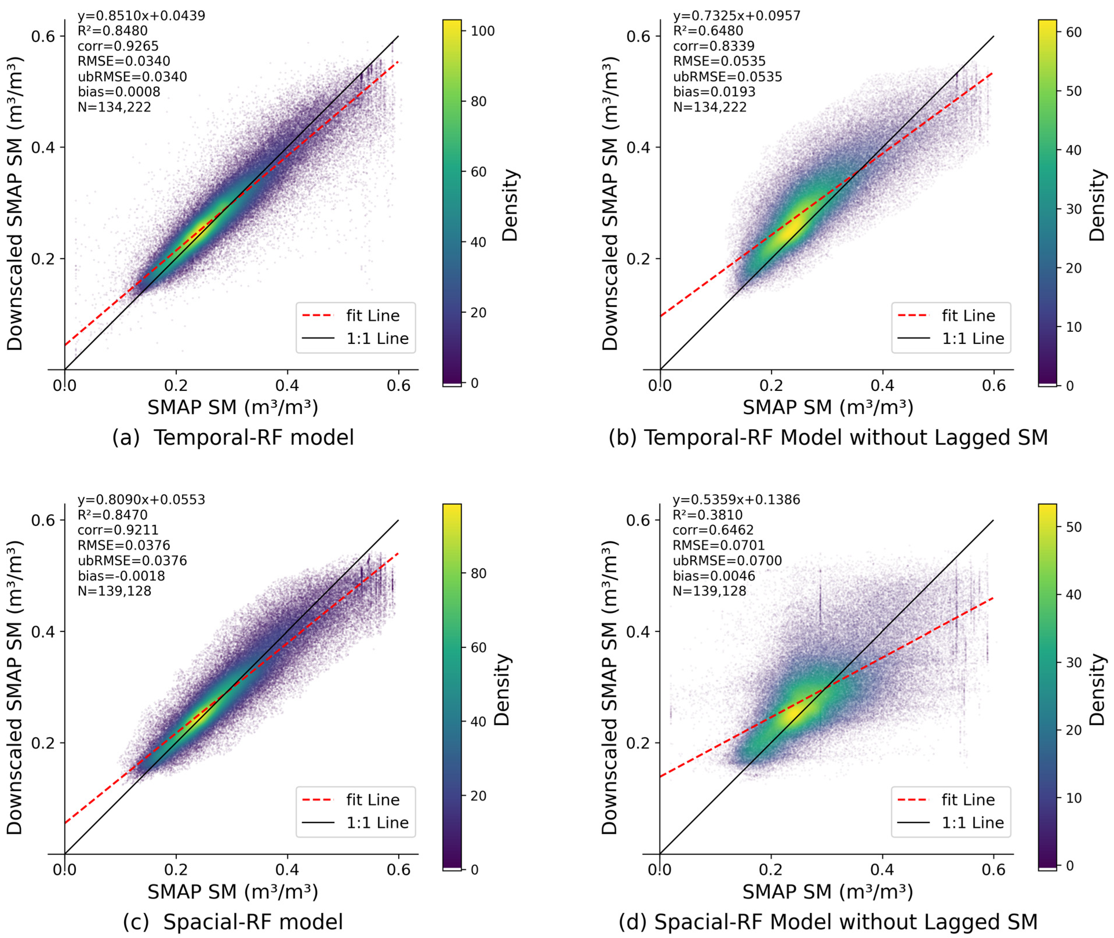
In this section, we first analyze the models’ performance on test sets. Figure 4 shows the scatter plot of the original SMAP SM and downscaled SM on test sets of each downscaling method. As is shown in the figure, the temporal model (model evaluated by the temporal splitting strategy) with lagged SM variables obtained the best performance in the test set. Its R2 was 0.848, both its RMSE and ubRMSE were 0.034 m3/m3, and its bias was 0.0008 m3/m3. Meanwhile, the R2 of spatial model (model evaluated by the spatial splitting strategy) with lagged SM variables reached 0.847, which was slightly lower than the temporal model with lagged SM. Both temporal and spatial models with lagged SM variables performed better than models without lagged SM variables. That is, the scatter-plot distributions for models without lagged SM in Figure 4b,d were more divergent than those for models with lagged SM in Figure 4a,c, and their metrics were worse. The performance of spatial model without lagged SM had the worst performance with a R2 of 0.381 among all models, which means that the spatial simulation of this model cannot meet the satisfying downscaling results in practice. In general, we can conclude that, compared with the previous common RF downscaling model, the downscaling model with lagged SM variables had improvement and maintained good performance in temporal and spatial evaluations. Because the temporal model with lagged SMs had similar performance with the spatial model with lagged SM, we chose to demonstrate the results of the temporal model with lagged SM only in the following discussion.

3.2. Roles of Variables in Downscaling SM

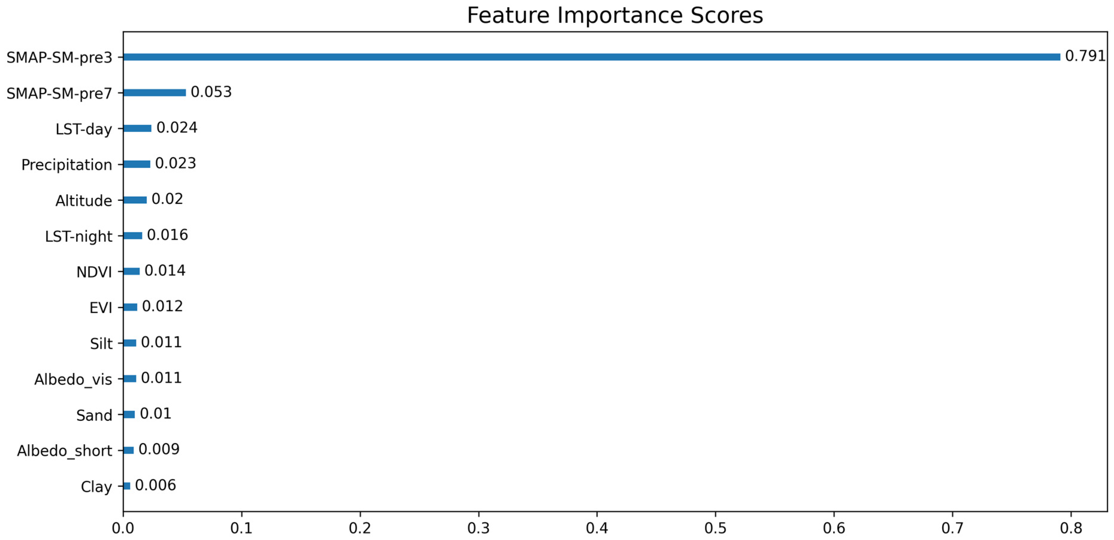
Figure 5 presents the feature importance rank of the temporal model with lagged SM variables. We can see that SMAP-SM-pre3 and SMAP-SM-pre7 variables that represent the three-day and seven-day lagged SM had the highest relative variable importance, which indicated that they had the largest contribution to reducing model error in the training process. This result mainly reflects the importance of lagged SM in reflecting SM temporal changes. Although the spatial resolution of the information provided by lagged SM is limited by the original SMAP SM products which cannot provide more spatial details, the average quality of the downscaling product in the 36-km grid is maintained by lagged SM variables. Thus, the downscaled data will not deviate too far from the original data. The lagged SM variables provide the basic simulated SM in the 36 km grids, and the spatial details are provided by other variables, such as LST-day, LST-night, precipitation and altitude presented in Figure 5. It is worth noting that the feature importance rank of the RF model indicates each variable′s average contribution to the prediction of the time series of the target variable in the training process; however, it cannot directly reflect the ability of each variable to provide spatial details.
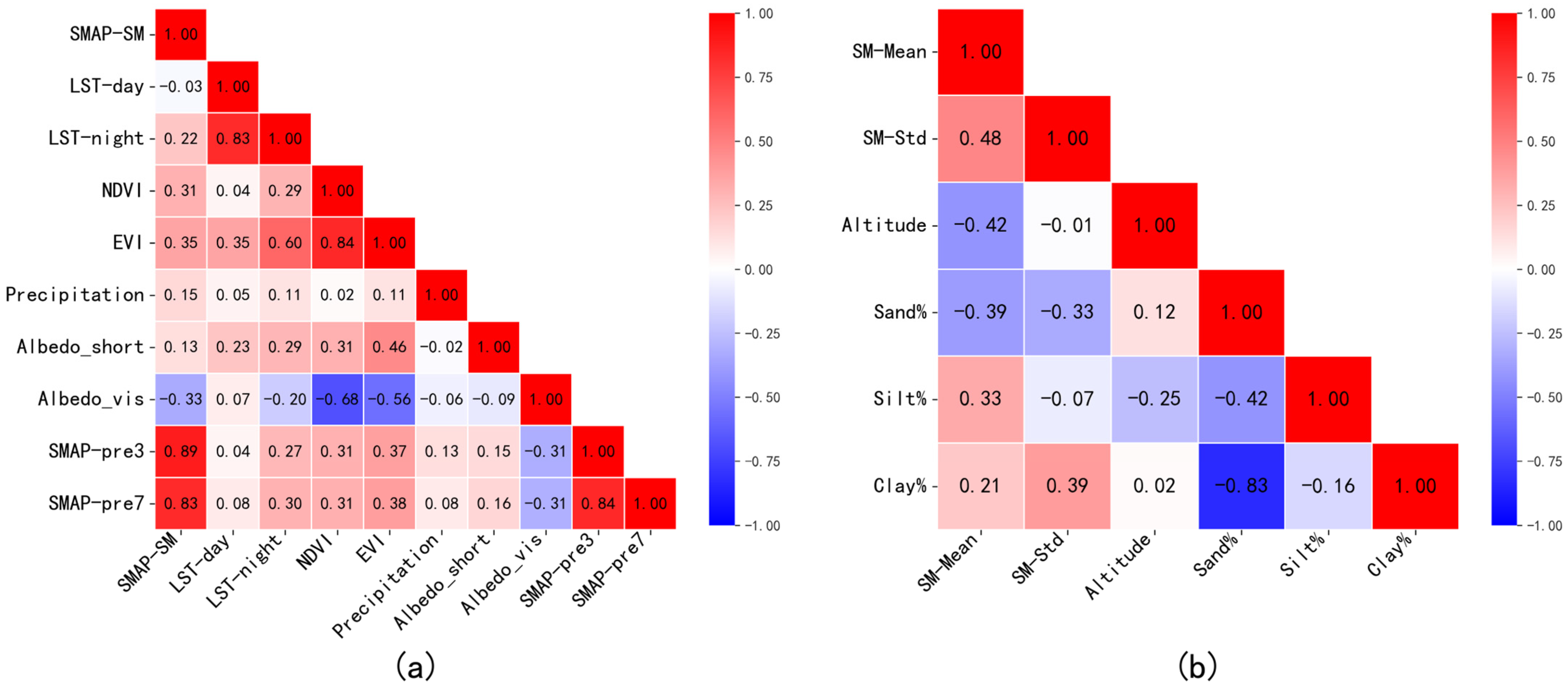
Figure 6a shows the mean r between dynamic variables. It should be noted that some small r values are still statistically significant (p < 0.001) due to the large sample size (13,422 samples in Figure 6a and 1166 samples in Figure 6b). We can see that the rank of r between each dynamic variable and SM in the training set is not completely consistent with the importance ranking in Figure 5, indicating that the importance rank of RF can not be used as the only indicator for variable relationship analysis. In Figure 6a, SMAP-SM-pre3 and SMAP-SM-pre7 variables correlated better with SM than other variables due to SM memory. However, the r of LST-day and precipitation variables with SMAP SM were low while these variables were third and fourth variables in the above rank of importance of variables.The r between SMAP SM and LST-night was higher than between SMAP SM and LST-day, which is consistent with previous findings [51]. In Figure 6b, The proportion of silt and clay had a positive r with mean SM, which is related to their good water storage capacity. Accordingly, the proportion of sand had negative r with mean SM and the standard deviation of SM, which should be caused by the low water-holding capacity of sand, similar to the results observed by Karthikeyan, L. et al. (2021) [68]. There was a relatively strong negative r between altitude and mean SM, but there was a small r between altitude and standard deviation of SM, so the influence of altitude on SM was more reflected in the mean climate state of SM. In general, we can know that most variables had a significant correlation with SM, and static variables had strong influences on the spatial distribution of SM rather than tempral change. Considering the fact that the r indicates the linear relationship between two variables, and the feature importance rank mainly reflects the nonlinear relationship of auxiliary variables, it is reasonable that there were some inconsistences between values′ rank in Figure 5 and Figure 6. The r and feature importance rank should be combined to analyze the importance of auxiliary variables.

3.3. Spatial Distribution of the Downscaled SM

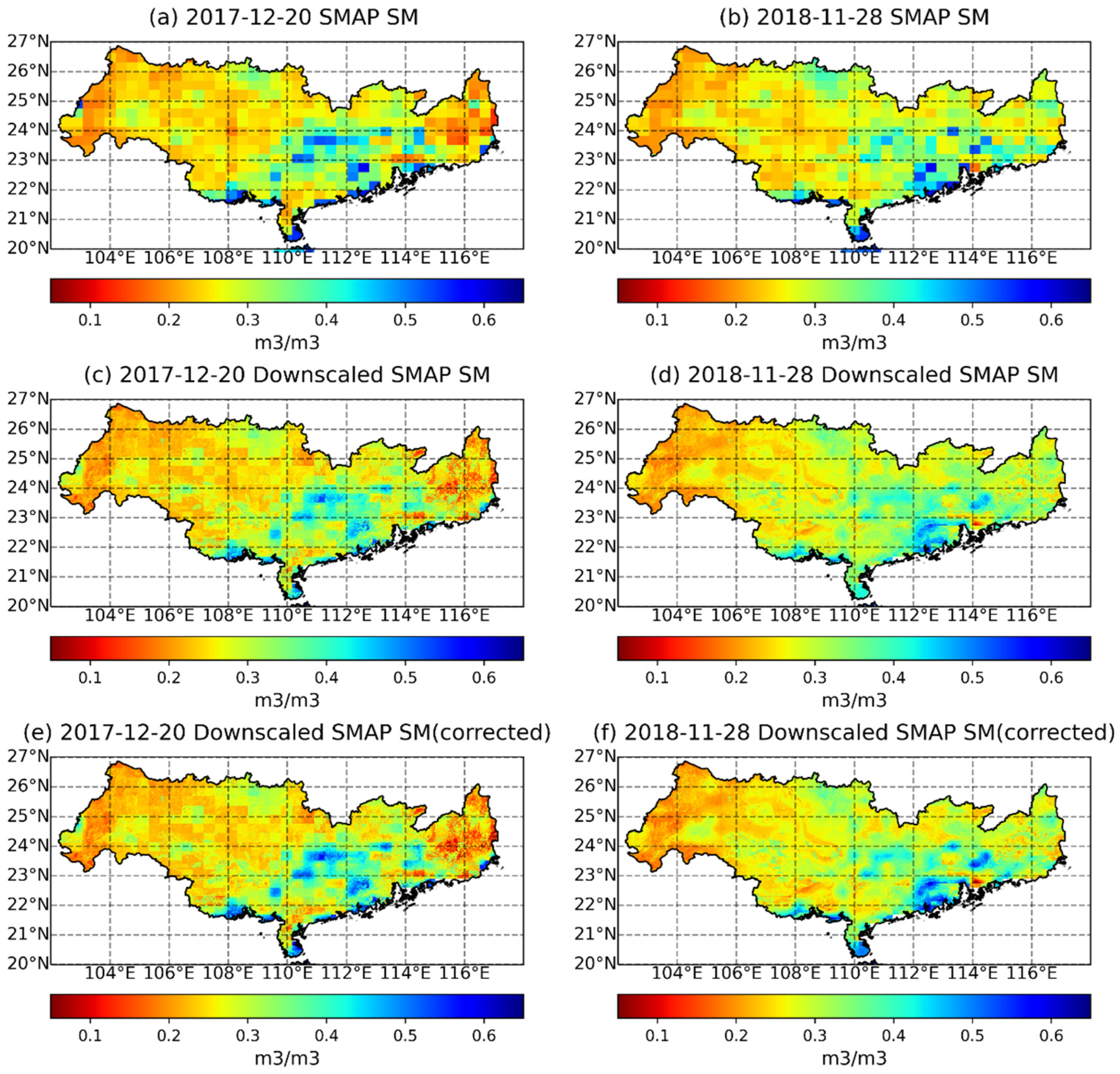
In Figure 7, we selected 20 December 2017 and 28 November 2018, in the test set of the temporal model to analyze the spatial distribution of downscaled SM. We selected these two sunny days to ensure the availability of MODIS data and SMAP data. It can be seen from Figure 7c,d that the distribution of downscaled SM was similar to the distribution of the original SMAP SM (Figure 7a,b), and the location of low and high value centers of downscaled SM matched well with the original SMAP SM. Downscaled SM showed more spatial details and was smoother than the original SMAP SM. It is worth noting that there was still some information loss on downscaled SM compared to the original SMAP SM, which appeared as the underestimation of high value and overestimation of low value in Figure 7c,d. This is because the downscaling model was built on the scale of a 36-km grid, and some extreme values were smoothed in the process of variable averaging [51]. To improve the above situation, we corrected downscaled SM by mass conservation. Figure 7e,f show the distribution of downscaled SM after correcting. We can see that the values of low and high center were more consistent with the original SMAP SM, and the original downscaling details were maintained at the same time, which indicates that using correction of mass conservation to downscaled SM can improve the information loss in downscaling process.
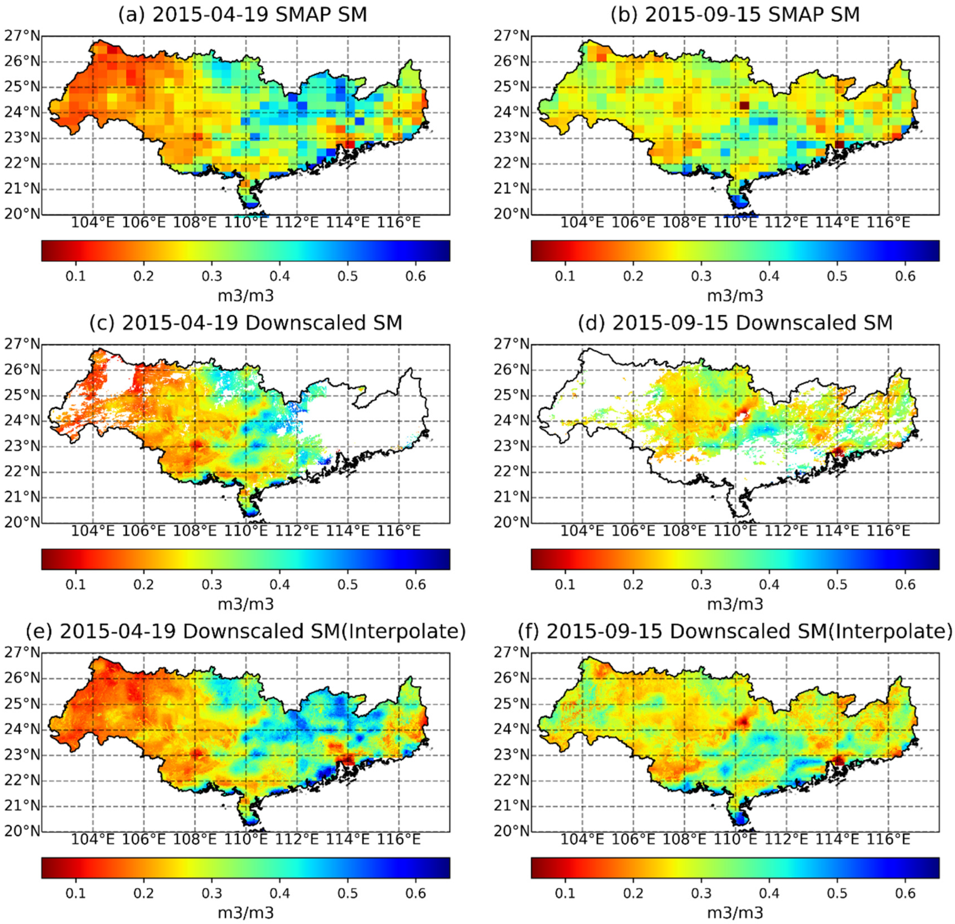
Meanwhile, two cloudy days, i.e., 20 December 2017 and 28 November 2018, were selected to study the effect of MODIS data missing due to cloud cover on downscaling model (Figure 8). Figure 8a,b are the original SMAP SM used as reference, Figure 8c–f are the distribution of downscaled SM. In Figure 8c,d, we can find there were many missing values in the picture because auxiliary variables data-derived from MODIS are missing due to cloud cover, and the downscaling model cannot downscale SM at the pixel where there was not enough auxiliary variable data. To fill up these missing values, we filled the missing MODIS variables data by linear interpolation in temporal dimension. Figure 8e,f show the distribution of downscaled SM after variables interpolation. Although linear interpolation cannot reflect the real values of auxiliary variables and will add errors to downscaling models, the distribution of downscaled SM after variables interpolation stills obtained good performance.

3.4. Validations by In Situ SM

The above analyses of results are mainly based on the test set of RF downscaling model. To further study the performance of the downscaled SM, we used in situ SM as a reference to validate the downscaled SM and the original SM in the following analysis.
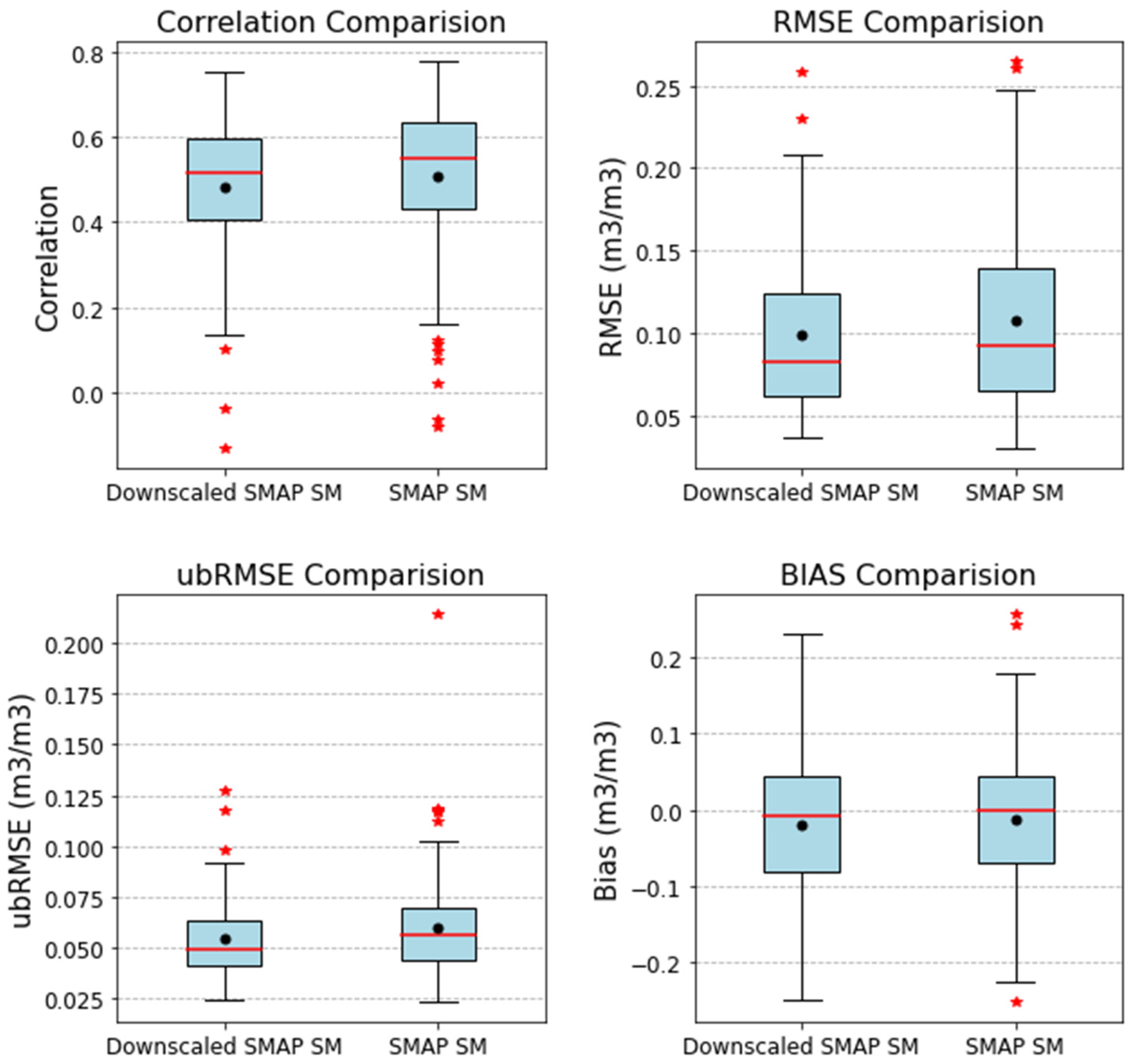
Figure 9 shows the comparison of in situ validations of 105 stations between the downscaled SM and the original SMAP SM. The validation results of the downscaled SM were basically close to those of SMAP SM. The median (0.52) and mean (0.49) of the r of the downscaled SM were slightly lower than those of SMAP SM data (median: 0.54, mean: 0.51). The RMSE of downscaled SM (median: 0.083 m3/m3, mean: 0.099 m3/m3) and the ubRMSE of downscaled SM (median: 0.049 m3/m3, mean: 0.055 m3/m3) were slightly lower than those of SMAP SM (median: 0.092 m3/m3, RMSE mean: 0.108 m3/m3; median ubRMSE: 0.056 m3/m3, ubRMSE mean: 0.06 m3/m3). As for bias comparison, the median and mean of downscaled SM were −0.009 m3/m3 and −0.02 m3/m3, both of which were larger than SMAP SM (median: −0.001 m3/m3 and mean: −0.013 m3/m3), indicating that downscaling data had certain bias amplification. The existence of relatively large bias provides a certain basis for the correction of mass conservation mentioned in Section 3.3.
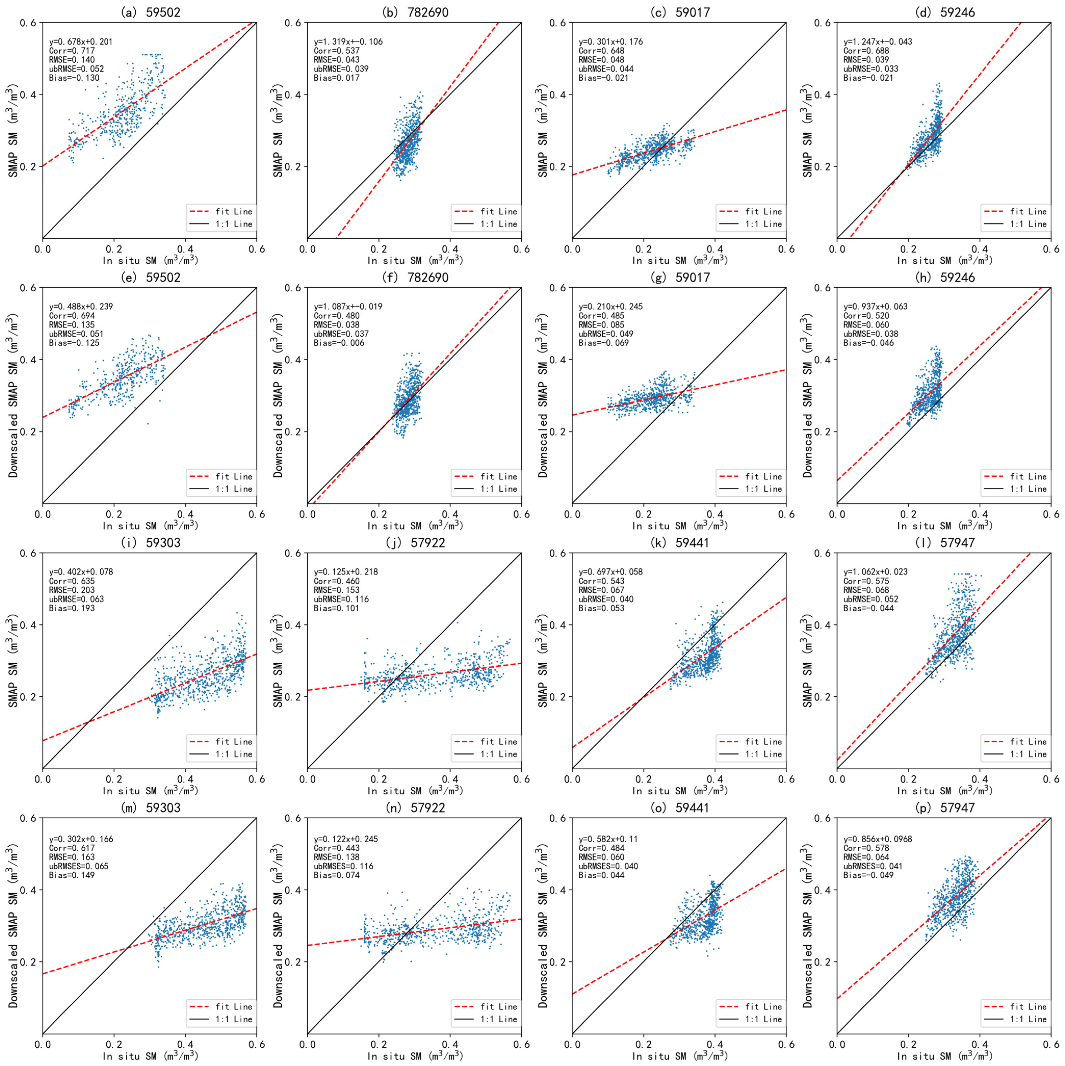
In Figure 10, eight stations (station number: 59502, 782690, 59017, 59249, 59303, 57922, 59441, 57947) were randomly selected to compare the downscaled SM and SMAP SM through drawing with in situ SM respectively. By comparing the scatters of downscaled SM and SMAP SM in corresponding stations, we can discover that the scatter distribution of the downscaled SM was basically consistent with that of SMAP SM, indicating that the downscaled SM retained most of the information of SMAP SM. Furthermore, the divergence degree of scatter distribution of the downscaled SM was smaller than that of SMAP SM, which was mainly reflected in fewer abnormal scatters and more concentrated scatters. This is consistent with Figure 9, which shows that the mean RMSE and ubRMSE of downscaled SM was lower than that of SMAP SM. In general, the downscaled SM maintained most information of the original SMAP SM and presented a reasonable distribution compared to the original SM.
Figure 11 shows the time series of the downscaled SM, SMAP SM, in situ SM and rainfall in four randomly selected stations (57955, 56697, 56985 and 57923). The time coverage of the time series is the date of the temporal model’s test set. It can be seen in Figure 11 that the temporal variation of downscaled (red points) was almost consistent with SMAP SM (blues points), which indicates that downscaled SM basically can capture the temporal change of SMAP SM, which is attributed to the addition of lagged SM variables into the downscaling model. At the same time, both SMAP SM and downscaled SM had a good response to precipitation, and both of them showed an increasing trend after precipitation occurred.
When there was a large bias between SMAP SM and in situ SM, the downscaled SM simulated based on SMAP SM also had a large bias compared to in situ SM, such as the green circle part in the figure and the whole time series of the second stations (56697). The SMAP SM and the downscaled SM in the green circle had relatively large deviations from in situ SM. In the whole time series of 56697 site, although the fluctuations of SMAP SM and the downscaled SM were consistent with that of in situ data, their values were lower than in situ SM, but it seems that the underestimation of the downscaled SM was smaller than the SMAP SM, which indicates that there may be some improvement of the downscaled SM at this station. In general, the performance of the downscaling SM validated by in situ SM was limited by the original SMAP SM as the downscaled SM maintained most information of SMAP SM, but there were still some improvements of the downscaled SM at some stations.

4. Discussion

From the comparison of downscaling models (Figure 4), we can find that downscaling models with lagged SM variables obtained good performance and basically meet the downscaling requirements. The R2 of the temporal model reached 0.848 and the R2 of the spatial model reached 0.847. Compared to downscaling models without lagged SM variables, our models with lagged SM variables had strong stabilities in temporal and spatial scales, which indicates that lagged SM variables brought great improvement to downscaling model. It can be seen in Figure 5 and Figure 6 that lagged SM variables plays a vital role in the importance rank of RF downscaling model, which can be used to explain the improvement of downscaling model: the lagged SM variables ensured the prediction quality on the 36-km grid by their strong temporal autocorrelation. The high temporal autocorrelation caused by SM memory provides a benchmark of prediction, which means that downscaled SM on each grid would not deviate too far from the original SMAP SM, while the finer spatial distribution was predicted by the information of other finer-resolution variables to meet the downscaling requirements. These variables such as LST, NDVI and albedo have been proved by previous studies that their temporal and spatial variations can strongly influence the distribution of SM [69,70,71].
In addition, from the comparison of the downscaled SM on selected sunny and cloudy days (Figure 7 and Figure 8), the downscaled SM under the two weather conditions had acceptable performance. It shows that the downscaling model maintained a certain stability in the absence of auxiliary variables under the impact of cloud cover. This may be explained by the fact that lagged SM variables ensured the quality of the 36-km grid in the average state; therefore, even if the MODIS variables had a certain deviation due to simple linear interpolation, the output downscaled SM would not have large bias, which further confirmed that the lagged SM variables can improve the downscaling model to some extent. However, the downscaled SM still had bias in the high and low values, which is a common problem of downscaling models because the variables were aggregated to 36 km by averaging, and the variation range of variables was smoothed [51]. This problem affects downscaling models, which may then output simulations that do not conform to the physical law: e.g., conservation of mass. However, this problem can be improved using simple post-processing of mass conservation correction (Figure 7). Similar correction methods were also applied in the studies of downscaling land surface temperature [72].
From the in situ validation for the downscaled SM and SMAP SM (Figure 9, Figure 10 and Figure 11), the downscaled SM retained most information of SMAP SM due to the great performance of the downscaling model. Therefore, the performance validated by in situ SM was also largely limited by the original SMAP SM, though there may be some improvements of the downscaled SM at some stations. It is reasonable that the performance of the downscaled SM was determined by the quality of the original SMAP SM, because SMAP SM was the training target of the RF downscaling model, and the output downscaled SM were predicted on the basis of the relationship between training target and auxiliary variables learned by RF downscaling model [37,73]. Additionally, there were still some experimental errors in in situ validation due to the different scales of the downscaled SM (1 km), in situ SM (point scale), and the SMAP SM (36 km), and depth difference between SMAP SM (0–5 cm) and in situ SM (10 cm).
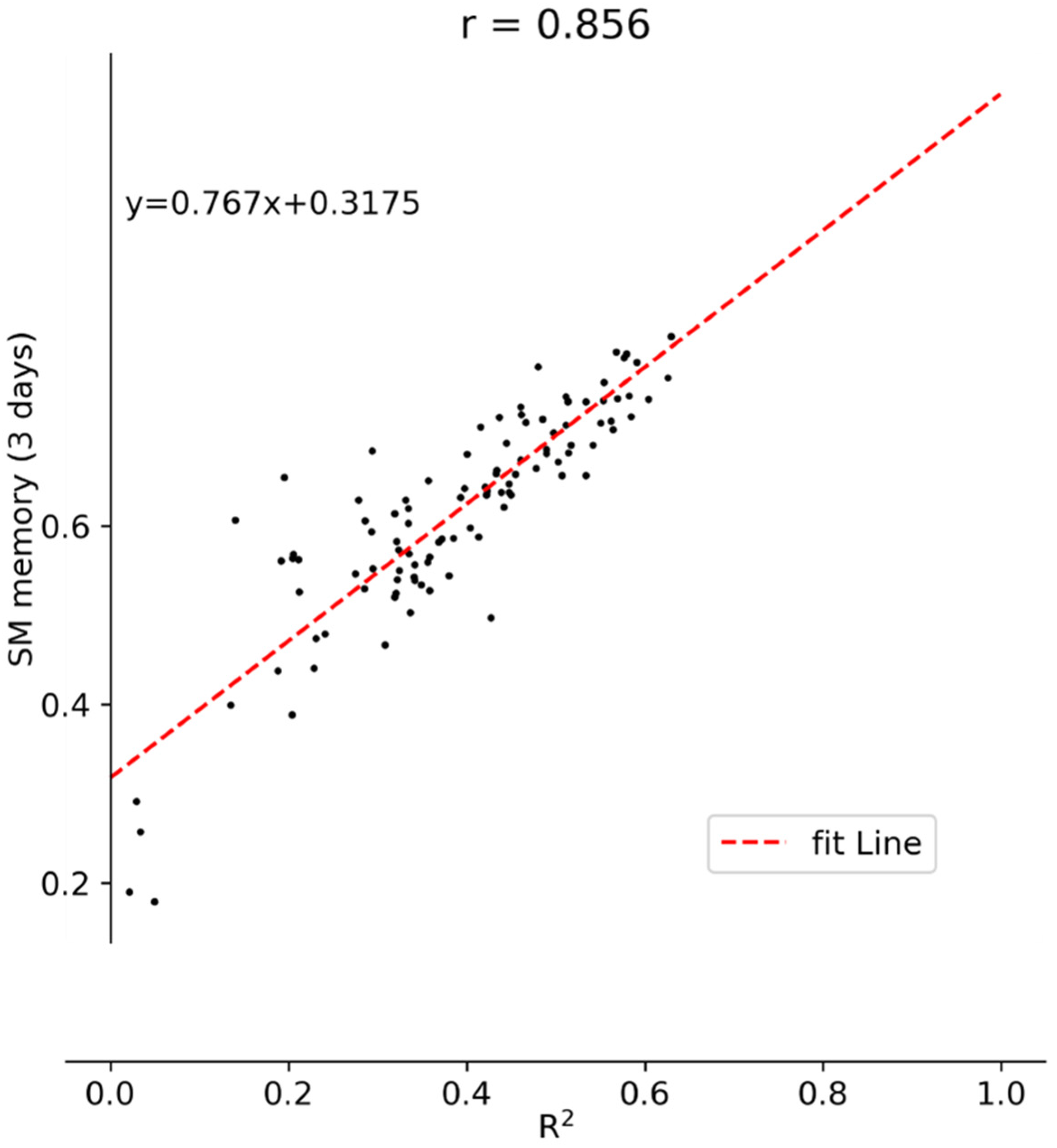
In order to discuss the influence of lagged SM variables, Figure 12 shows the relationship between the model performance measured by R2 and SM memory representing by the three-day lagged autocorrelation at each grid. It can be seen from the figure that there is an obvious positive correlation (0.856) between soil moisture memory and downscaling model performance. The better the soil moisture memory, the better the downscaling performs. This coincides well with previous studies [44].
There are still some shortcomings in this work. First, there is a mismatch problem of the spatial scale of different data when the downscaling model is constructed and verified. When the model is constructed, the fine resolution variables were averaged to match SMAP SM, which leads to errors; uncertainty was introduced by the direct comparison of in situ SM (point scale) and grid data in the validation experiment. Second, due to the different sensor types and inversion algorithms used in multi-source data, the uncertainty of the model increased. At the same time, although the remote sensing data is quality controlled, they will still be affected by cloud covers, resulting in errors or even missing values. Interpolation of these remote sensing data added errors to the model [50,73]. Third, some variables of the downscaling model, such as NDVI and EVI, are nonlinear indicators, but they were directly averaged to aggregate to the resolution of 36 km, which may produce errors and reduce the performance of the model. Finally, due to the limitation of the study area, the downscaling model did not have sufficient train samples to study more extreme cases and spatial patterns.

5. Conclusions

The novelty of this paper has two major aspects: the usage of the lagged SM and the mass conservation correction. The downscaling model with lagged SM variables was built and compared with a typical machine learning downscaling model without lagged SM variables. We also studied whether the correction of mass conservation can be applied to output downscaled SM and its influence on the outcomes. Finally, we validated the downscaled SM by in situ SM and compared its validation with the original SMAP SM. The conclusions are as follows:
(1)
Lagged SM variables and the mass conservation correction can improve the performance of the downscaling model. From the features importance ranking and correlation coefficient analysis of the model, it can be concluded that the lagged SM variables are very important for the downscaling model.
(2)
The lagged SM variables provide the basis of SM in the original grids, and the spatial details are provided by high resolution static and time series data, including LST, precipitation, topography, NDVI and so on.
(3)
The improved downscaling model can not only output more spatial distribution details and more accurate SM, but it also has a certain interpolation ability so that the model can still reasonably predict the spatial distribution of SM in cloudy weather.
(4)
From the comparison of in situ validation, the downscaled SM retains most of the information of the original SMAP SM, though the performance of the downscaling SM is largely limited by the original SMAP SM. However, in some areas, the validation performance of the downscaled SM may be slightly better than that of the original SMAP SM.
In general, the research findings proposed in this work can provide some reference values for the improvement of the SM downscaling model, which is significant to the development of high-resolution SM information. However, there are still some aspects to be improved. First, more samples and larger research areas are needed to optimize the machine learning model and the proposed model needs to be applied and validated in other areas. Second, in situ SM data should be upscaled to match the scale of grid data to reduce the uncertainty in validation. Third, the gap filling method should be developed to improve the lack of remote sensing variables, and better related auxiliary variables should be explored to improve the downscaling model. Fourth, some nonlinear auxiliary variables such as NDVI and EVI were directly averaged to aggregate to the resolution of 36 km, which may produce errors and reduce the performance of the model. The aggregation method of these variables needs to be optimized. Last but not the least, the proposed model should be tested and applied with other SM products.

Author Contributions

Conceptualization, W.S.; methodology, T.M. and W.S.; validation, J.L., T.M. and W.S.; formal analysis, W.S. and T.M.; investigation, W.S., Q.L. and T.M.; writing—original draft preparation, T.M.; writing—review and editing, W.S., T.M., W.L., Y.Z. and F.H.; visualization, T.M., L.L. and R.Z.; supervision, W.S.; project administration, W.S.; funding acquisition, W.S. All authors have read and agreed to the published version of the manuscript.

Funding

This research was funded by the National Natural Science Foundation of China under Grants 41975122, U1811464, and 42088101, the National Key R&D Program of China under Grant 2017YFA0604300, the Innovation Group Project of Southern Marine Science and Engineering Guangdong Laboratory (Zhuhai) (311020008), and the Fundamental Research Funds for the Central Universities, Sun Yat-sen University.

Data Availability Statement

SMAP data can be downloaded from the website of the National Snow and Ice Data Center (NSIDC, https://nsidc.org/data/SPL3SMP). The in situ soil moisture data is available at http://data.cma.cn with certain permissions. The ERA5-Land dataset is available at https://cds.climate.copernicus.eu/cdsapp#!/dataset/reanalysis-era5-land?tab=form. The MODIS data can be obtained from the official website of MODIS (https://modis.gsfc.nasa.gov). The Chinese soil properties dataset can be obtained at http://globalchange.bnu.edu.cn (all accessed on 15 June 2022).

Acknowledgments

The authors thank the anonymous reviewers for providing such valuable comments.

Conflicts of Interest

The authors declare no conflict of interest.

References

  1. Seneviratne, S.I.; Corti, T.; Davin, E.L.; Hirschi, M.; Jaeger, E.B.; Lehner, I.; Orlowsky, B.; Teuling, A.J. Investigating Soil Moisture-Climate Interactions in a Changing Climate: A Review. Earth-Sci. Rev. 2010, 99, 125–161. [Google Scholar] [CrossRef]
  2. Koster, R.D.; Dirmeyer, P.A.; Guo, Z.; Bonan, G.; Chan, E.; Cox, P.; Gordon, C.T.; Kanae, S.; Kowalczyk, E.; Lawrence, D.; et al. Regions of Strong Coupling Between Soil Moisture and Precipitation. Science 2004, 305, 1138–1140. [Google Scholar] [CrossRef] [PubMed] [Green Version]
  3. Robinson, D.A.; Campbell, C.S.; Hopmans, J.W.; Hornbuckle, B.K.; Jones, S.B.; Knight, R.; Ogden, F.; Selker, J.; Wendroth, O. Soil Moisture Measurement for Ecological and Hydrological Watershed-Scale Observatories: A Review. Vadose Zone J. 2008, 7, 358–389. [Google Scholar] [CrossRef] [Green Version]
  4. Bolten, J.D.; Crow, W.T.; Zhan, X.; Jackson, T.J.; Reynolds, C.A. Evaluating the Utility of Remotely Sensed Soil Moisture Retrievals for Operational Agricultural Drought Monitoring. IEEE J. Sel. Top. Appl. Earth Obs. Remote Sens. 2009, 3, 57–66. [Google Scholar] [CrossRef] [Green Version]
  5. Dobriyal, P.; Qureshi, A.; Badola, R.; Hussain, S.A. A Review of the Methods Available for Estimating Soil Moisture and Its Implications for Water Resource Management. J. Hydrol. 2012, 458, 110–117. [Google Scholar] [CrossRef]
  6. Renzullo, L.J.; Van Dijk, A.; Perraud, J.-M.; Collins, D.; Henderson, B.; Jin, H.; Smith, A.B.; McJannet, D.L. Continental Satellite Soil Moisture Data Assimilation Improves Root-Zone Moisture Analysis for Water Resources Assessment. J. Hydrol. 2014, 519, 2747–2762. [Google Scholar] [CrossRef]
  7. Dirmeyer, P.A.; Wu, J.; Norton, H.E.; Dorigo, W.A.; Quiring, S.M.; Ford, T.W.; Santanello, J.A., Jr.; Bosilovich, M.G.; Ek, M.B.; Koster, R.D.; et al. Confronting Weather and Climate Models with Observational Data from Soil Moisture Networks over the United States. J. Hydrometeorol. 2016, 17, 1049–1067. [Google Scholar] [CrossRef]
  8. Tuttle, S.; Salvucci, G. Empirical Evidence of Contrasting Soil Moisture–Precipitation Feedbacks across the United States. Science 2016, 352, 825–828. [Google Scholar] [CrossRef] [Green Version]
  9. Ray, R.L.; Jacobs, J.M.; Cosh, M.H. Landslide Susceptibility Mapping Using Downscaled AMSR-E Soil Moisture: A Case Study from Cleveland Corral, California, US. Remote Sens. Environ. 2010, 114, 2624–2636. [Google Scholar] [CrossRef]
  10. Peng, J.; Shen, H.; He, S.W.; Wu, J.S. Soil Moisture Retrieving Using Hyperspectral Data with the Application of Wavelet Analysis. Environ. Earth Sci. 2013, 69, 279–288. [Google Scholar] [CrossRef]
  11. Petropoulos, G.P.; Ireland, G.; Barrett, B. Surface Soil Moisture Retrievals from Remote Sensing: Current Status, Products & Future Trends. Phys. Chem. Earth Parts A B C 2015, 83, 36–56. [Google Scholar]
  12. Robock, A.; Vinnikov, K.Y.; Srinivasan, G.; Entin, J.K.; Hoiiinger, S.E.; Speranskaya, N.A.; Liu, S.; Namkhai, A. The Global Soil Moisture Data Bank. Bull. Am. Meteorol. Soc. 2000, 81, 1281–1300. [Google Scholar] [CrossRef] [Green Version]
  13. Vinnikov, K.Y.; Yeserkepova, I.B. Soil Moisture: Empirical Data and Model Results. J. Clim. 1991, 4, 66–79. [Google Scholar] [CrossRef] [Green Version]
  14. Hollinger, S.E.; Isard, S.A. A Soil Moisture Climatology of Illinois. J. Clim. 1994, 7, 822–833. [Google Scholar] [CrossRef] [Green Version]
  15. Robinson, D.A.; Jones, S.B.; Wraith, J.M.; Or, D.; Friedman, S.P. A Review of Advances in Dielectric and Electrical Conductivity Measurement in Soils Using Time Domain Reflectometry. Vadose Zone J. 2003, 2, 444–475. [Google Scholar] [CrossRef]
  16. Owe, M.; de Jeu, R.; Holmes, T. Multisensor Historical Climatology of Satellite-derived Global Land Surface Moisture. J. Geophys. Res. Earth Surf. 2008, 113, F01002. [Google Scholar] [CrossRef]
  17. Entekhabi, D.; Njoku, E.G.; O’Neill, P.E.; Kellogg, K.H.; Crow, W.T.; Edelstein, W.N.; Entin, J.K.; Goodman, S.D.; Jackson, T.J.; Johnson, J. The Soil Moisture Active Passive (SMAP) Mission. Proc. IEEE 2010, 98, 704–716. [Google Scholar] [CrossRef]
  18. Jacquette, E.; Al Bitar, A.; Mialon, A.; Kerr, Y.; Quesney, A.; Cabot, F.; Richaume, P. SMOS CATDS Level 3 Global Products over Land. In Remote Sensing for Agriculture, Ecosystems, and Hydrology XII.; International Society for Optics and Photonics: Washington, DC, USA, 2010; Volume 7824, p. 78240K. [Google Scholar]
  19. Chauhan, N.S.; Miller, S.; Ardanuy, P. Spaceborne Soil Moisture Estimation at High Resolution: A Microwave-Optical/IR Synergistic Approach. Int. J. Remote Sens. 2003, 24, 4599–4622. [Google Scholar] [CrossRef]
  20. Piles, M.; Camps, A.; Vall-Llossera, M.; Sánchez, N.; Martínez-Fernández, J.; Monerris, A.; Baroncini-Turricchia, G.; Pérez-Gutiérrez, C.; Aguasca, A.; Acevo, R. Soil Moisture Downscaling Activities at the REMEDHUS Cal/Val Site and Its Application to SMOS. In Proceedings of the 2010 11th Specialist Meeting on Microwave Radiometry and Remote Sensing of the Environment, Washington, DC, USA, 1–4 March 2010; IEEE: New York, NY, USA, 2010; pp. 17–21. [Google Scholar]
  21. Zhan, X.; Miller, S.; Chauhan, N.; Di, L.; Ardanuy, P. Soil Moisture Visible/Infrared Radiometer Suite Algorithm Theoretical Basis Document; Raytheon Systems Company: Lanham, MD, USA, 2002. [Google Scholar]
  22. Merlin, O.; Chehbouni, A.; Walker, J.P.; Panciera, R.; Kerr, Y.H. A Simple Method to Disaggregate Passive Microwave-Based Soil Moisture. IEEE Trans. Geosci. Remote Sens. 2008, 46, 786–796. [Google Scholar] [CrossRef] [Green Version]
  23. Merlin, O.; Walker, J.P.; Chehbouni, A.; Kerr, Y. Towards Deterministic Downscaling of SMOS Soil Moisture Using MODIS Derived Soil Evaporative Efficiency. Remote. Sens. Environ. 2008, 112, 3935–3946. [Google Scholar] [CrossRef] [Green Version]
  24. Ke, Y.; Im, J.; Park, S.; Gong, H. Downscaling of MODIS One Kilometer Evapotranspiration Using Landsat-8 Data and Machine Learning Approaches. Remote Sens. 2016, 8, 215. [Google Scholar] [CrossRef] [Green Version]
  25. Im, J.; Park, S.; Rhee, J.; Baik, J.; Choi, M. Downscaling of AMSR-E Soil Moisture with MODIS Products Using Machine Learning Approaches. Environ. Earth Sci. 2016, 75, 1120. [Google Scholar] [CrossRef]
  26. Peng, J.; Loew, A.; Merlin, O.; Verhoest, N.E.C. A Review of Spatial Downscaling of Satellite Remotely Sensed Soil Moisture. Rev. Geophys. 2017, 55, 341–366. [Google Scholar] [CrossRef]
  27. Piles, M.; Petropoulos, G.P.; Sánchez, N.; González-Zamora, Á.; Ireland, G. Towards Improved Spatio-Temporal Resolution Soil Moisture Retrievals from the Synergy of SMOS and MSG SEVIRI Spaceborne Observations. Remote Sens. Environ. 2016, 180, 403–417. [Google Scholar] [CrossRef] [Green Version]
  28. Zhao, W.; Li, A. A Downscaling Method for Improving the Spatial Resolution of AMSR-E Derived Soil Moisture Product Based on MSG-SEVIRI Data. Remote Sens. 2013, 5, 6790–6811. [Google Scholar] [CrossRef] [Green Version]
  29. Zhao, W.; Li, A.; Jin, H.; Zhang, Z.; Bian, J.; Yin, G. Performance Evaluation of the Triangle-Based Empirical Soil Moisture Relationship Models Based on Landsat-5 TM Data and in Situ Measurements. IEEE Trans. Geosci. Remote Sens. 2017, 55, 2632–2645. [Google Scholar] [CrossRef]
  30. Zhao, W.; Li, A. A Comparison Study on Empirical Microwave Soil Moisture Downscaling Methods Based on the Integration of Microwave-Optical/IR Data on the Tibetan Plateau. Int. J. Remote Sens. 2015, 36, 4986–5002. [Google Scholar] [CrossRef]
  31. Abbaszadeh, P.; Moradkhani, H.; Zhan, X. Downscaling SMAP Radiometer Soil Moisture Over the CONUS Using an Ensemble Learning Method. Water Resour. Res. 2019, 55, 324–344. [Google Scholar] [CrossRef] [Green Version]
  32. Long, D.; Bai, L.; Yan, L.; Zhang, C.; Yang, W.; Lei, H.; Quan, J.; Meng, X.; Shi, C. Generation of Spatially Complete and Daily Continuous Surface Soil Moisture of High Spatial Resolution. Remote Sens. Environ. 2019, 233, 111364. [Google Scholar] [CrossRef]
  33. Pelletier, C.; Valero, S.; Inglada, J.; Champion, N.; Dedieu, G. Assessing the Robustness of Random Forests to Map Land Cover with High Resolution Satellite Image Time Series over Large Areas. Remote Sens. Environ. 2016, 187, 156–168. [Google Scholar] [CrossRef]
  34. Peng, J.; Loew, A.; Zhang, S.; Wang, J.; Niesel, J. Spatial Downscaling of Satellite Soil Moisture Data Using a Vegetation Temperature Condition Index. IEEE Trans. Geosci. Remote Sens. 2015, 54, 558–566. [Google Scholar] [CrossRef]
  35. Teluguntla, P.; Thenkabail, P.S.; Oliphant, A.; Xiong, J.; Gumma, M.K.; Congalton, R.G.; Yadav, K.; Huete, A. A 30-m Landsat-Derived Cropland Extent Product of Australia and China Using Random Forest Machine Learning Algorithm on Google Earth Engine Cloud Computing Platform. ISPRS J. Photogramm. Remote Sens. 2018, 144, 325–340. [Google Scholar] [CrossRef]
  36. Wei, Z.; Meng, Y.; Zhang, W.; Peng, J.; Meng, L. Downscaling SMAP Soil Moisture Estimation with Gradient Boosting Decision Tree Regression over the Tibetan Plateau. Remote Sens. Environ. 2019, 225, 30–44. [Google Scholar] [CrossRef]
  37. Liu, Y.; Jing, W.; Wang, Q.; Xia, X. Generating High-Resolution Daily Soil Moisture by Using Spatial Downscaling Techniques: A Comparison of Six Machine Learning Algorithms. Adv. Water Resour. 2020, 141, 103601. [Google Scholar] [CrossRef]
  38. Djamai, N.; Magagi, R.; Goïta, K.; Merlin, O.; Kerr, Y.; Roy, A. A Combination of DISPATCH Downscaling Algorithm with CLASS Land Surface Scheme for Soil Moisture Estimation at Fine Scale during Cloudy Days. Remote Sens. Environ. 2016, 184, 1–14. [Google Scholar] [CrossRef]
  39. Molero, B.; Merlin, O.; Malbéteau, Y.; Al Bitar, A.; Cabot, F.; Stefan, V.; Kerr, Y.; Bacon, S.; Cosh, M.H.; Bindlish, R. SMOS Disaggregated Soil Moisture Product at 1 Km Resolution: Processor Overview and First Validation Results. Remote Sens. Environ. 2016, 180, 361–376. [Google Scholar] [CrossRef]
  40. McColl, K.A.; Alemohammad, S.H.; Akbar, R.; Konings, A.G.; Yueh, S.; Entekhabi, D. The Global Distribution and Dynamics of Surface Soil Moisture. Nat. Geosci. 2017, 10, 100–104. [Google Scholar] [CrossRef]
  41. Hong, Z.; Kalbarczyk, Z.; Iyer, R.K. A Data-Driven Approach to Soil Moisture Collection and Prediction. In Proceedings of the 2016 IEEE International Conference on Smart Computing (SMARTCOMP), St. Louis, MO, USA, 18–20 May 2016; IEEE: New York, NY, USA, 2016; pp. 1–6. [Google Scholar]
  42. Zaman, B.; McKee, M. Spatio-Temporal Prediction of Root Zone Soil Moisture Using Multivariate Relevance Vector Machines. Open J. Mod. Hydrol. 2014, 4, 80. [Google Scholar] [CrossRef] [Green Version]
  43. Carranza, C.; Nolet, C.; Pezij, M.; van der Ploeg, M. Root Zone Soil Moisture Estimation with Random Forest. J. Hydrol. 2021, 593, 125840. [Google Scholar] [CrossRef]
  44. Pan, J.; Shangguan, W.; Li, L.; Yuan, H.; Zhang, S.; Lu, X.; Wei, N.; Dai, Y. Using Data-Driven Methods to Explore the Predictability of Surface Soil Moisture with FLUXNET Site Data. Hydrol. Process. 2019, 33, 2978–2996. [Google Scholar] [CrossRef]
  45. Pearl River Water Resources Committee (PRWRC). The Zhujiang Archive; Guandong Science and Technology Press: Guangzhou, China, 1991; Volume 1. [Google Scholar]
  46. Zhang, Q.; Xu, C.; Gemmer, M.; Chen, Y.D.; Liu, C. Changing Properties of Precipitation Concentration in the Pearl River Basin, China. Stoch. Environ. Res. Risk Assess. 2009, 23, 377–385. [Google Scholar] [CrossRef]
  47. O’Neill, P.E.; Chan, S.; Njoku, E.G.; Jackson, T.; Bindlish, R.; Chaubell, J. SMAP L3 Radiometer Global Daily 36 km EASE-Grid Soil Moisture, Version 8; NASA National Snow and Ice Data Center Distributed Active Archive Center: Boulder, CO, USA, 2021. [CrossRef]
  48. Chen, Q.; Zeng, J.; Cui, C.; Li, Z.; Chen, K.-S.; Bai, X.; Xu, J. Soil Moisture Retrieval from SMAP: A Validation and Error Analysis Study Using Ground-Based Observations over the Little Washita Watershed. IEEE Trans. Geosci. Remote Sens. 2017, 56, 1394–1408. [Google Scholar] [CrossRef]
  49. Colliander, A.; Jackson, T.J.; Bindlish, R.; Chan, S.; Das, N.; Kim, S.B.; Cosh, M.H.; Dunbar, R.S.; Dang, L.; Pashaian, L. Validation of SMAP Surface Soil Moisture Products with Core Validation Sites. Remote Sens. Environ. 2017, 191, 215–231. [Google Scholar] [CrossRef]
  50. Zhao, W.; Sánchez, N.; Lu, H.; Li, A. A Spatial Downscaling Approach for the SMAP Passive Surface Soil Moisture Product Using Random Forest Regression. J. Hydrol. 2018, 563, 1009–1024. [Google Scholar] [CrossRef]
  51. Dorigo, W.A.; Xaver, A.; Vreugdenhil, M.; Gruber, A.; Hegyiová, A.; Sanchis-Dufau, A.D.; Zamojski, D.; Cordes, C.; Wagner, W.; Drusch, M. Global Automated Quality Control of In Situ Soil Moisture Data from the International Soil Moisture Network. Vadose Zone J. 2013, 12, vzj2012.0097. [Google Scholar] [CrossRef]
  52. Wan, Z.; Hook, S.; Hulley, G. MODIS/Terra Land Surface Temperature/Emissivity Daily L3 Global 1 km SIN Grid V061. NASA EOSDIS Land Processes DAAC. Available online: https://lpdaac.usgs.gov/products/mod11a1v061/ (accessed on 23 June 2022).
  53. Didan, K. MODIS/Terra Vegetation Indices 16-Day L3 Global 1 km SIN Grid V061. NASA EOSDIS Land Processes DAAC. Available online: https://lpdaac.usgs.gov/products/mod13a2v061/ (accessed on 23 June 2022).
  54. Schaaf, C.; Wang, Z. MODIS/Terra + Aqua BRDF/Albedo Daily L3 Global—500 m V061. NASA EOSDIS Land Processes DAAC. Available online: https://lpdaac.usgs.gov/products/mcd43a3v061/ (accessed on 6 April 2022).
  55. Lewis, P.; Barnsley, M.J. Influence of the Sky Radiance Distribution on Various Formulations of the Earth Surface Albedo. In Proceedings of the 6th International Symposium on Physical Measurements and Signatures in Remote Sensing, ISPRS, Val d’Isere, France, 17–21 January 1994; CNES: Tolouse, France, 1994; pp. 707–715. [Google Scholar]
  56. Sabater, J.M. ERA5-Land Hourly Data from 1981 to Present, Copernicus Climate Change Service (C3S) Climate Data Store (CDS) [Data Set]; Copernicus Climate Data Store: Brussels, Belgium, 2019. [Google Scholar]
  57. Sabater, J.M. ERA5-Land Hourly Data from 1950 to 1980, Copernicus Climate Change Service (C3S) Climate Data Store (CDS) [Data Set]; Copernicus Climate Data Store: Brussels, Belgium, 2021. [Google Scholar]
  58. Dai, Y.; Zeng, X.; Dickinson, R.E.; Baker, I.; Bonan, G.B.; Bosilovich, M.G.; Denning, A.S.; Dirmeyer, P.A.; Houser, P.R.; Niu, G. The Common Land Model. Bull. Am. Meteorol. Soc. 2003, 84, 1013–1024. [Google Scholar] [CrossRef] [Green Version]
  59. Shangguan, W.; Dai, Y.; Liu, B.; Zhu, A.; Duan, Q.; Wu, L.; Ji, D.; Ye, A.; Yuan, H.; Zhang, Q.; et al. A China Data Set of Soil Properties for Land Surface Modeling. J. Adv. Model. Earth Syst. 2013, 5, 212–224. [Google Scholar] [CrossRef]
  60. Crow, W.T.; Berg, A.A.; Cosh, M.H.; Loew, A.; Mohanty, B.P.; Panciera, R.; De Rosnay, P.; Ryu, D.; Walker, J.P. Upscaling Sparse Ground-Based Soil Moisture Observations for the Validation of Coarse-Resolution Satellite Soil Moisture Products. Rev. Geophys. 2012, 50, RG2002. [Google Scholar] [CrossRef] [Green Version]
  61. Ranney, K.J.; Niemann, J.D.; Lehman, B.M.; Green, T.R.; Jones, A.S. A Method to Downscale Soil Moisture to Fine Resolutions Using Topographic, Vegetation, and Soil Data. Adv. Water Resour. 2015, 76, 81–96. [Google Scholar] [CrossRef] [Green Version]
  62. Busch, F.A.; Niemann, J.D.; Coleman, M. Evaluation of an Empirical Orthogonal Function–Based Method to Downscale Soil Moisture Patterns Based on Topographical Attributes. Hydrol. Process. 2012, 26, 2696–2709. [Google Scholar] [CrossRef]
  63. Coleman, M.L.; Niemann, J.D. Controls on Topographic Dependence and Temporal Instability in Catchment-scale Soil Moisture Patterns. Water Resour. Res. 2013, 49, 1625–1642. [Google Scholar] [CrossRef]
  64. Mascaro, G.; Vivoni, E.R.; Deidda, R. Soil Moisture Downscaling across Climate Regions and Its Emergent Properties. J. Geophys. Res. Atmos. 2011, 116, D22114. [Google Scholar] [CrossRef] [Green Version]
  65. NASA JPL. NASA Shuttle Radar Topography Mission Global 3 Arc Second Number. NASA EOSDIS Land Processes DAAC. Available online: https://lpdaac.usgs.gov/products/srtmgl3nv003/ (accessed on 23 June 2022).
  66. Breiman, L. Random Forests. Mach. Learn. 2001, 45, 5–32. [Google Scholar] [CrossRef] [Green Version]
  67. Hu, F.; Wei, Z.; Zhang, W.; Dorjee, D.; Meng, L. A Spatial Downscaling Method for SMAP Soil Moisture through Visible and Shortwave-Infrared Remote Sensing Data. J. Hydrol. 2020, 590, 125360. [Google Scholar] [CrossRef]
  68. Karthikeyan, L.; Mishra, A.K. Multi-Layer High-Resolution Soil Moisture Estimation Using Machine Learning over the United States. Remote. Sens. Environ. 2021, 266, 112706. [Google Scholar] [CrossRef]
  69. Ghanbarian, B.; Taslimitehrani, V.; Dong, G.; Pachepsky, Y.A. Sample Dimensions Effect on Prediction of Soil Water Retention Curve and Saturated Hydraulic Conductivity. J. Hydrol. 2015, 528, 127–137. [Google Scholar] [CrossRef] [Green Version]
  70. Giraldo, M.A.; Bosch, D.; Madden, M.; Usery, L.; Finn, M. Ground and Surface Temperature Variability for Remote Sensing of Soil Moisture in a Heterogeneous Landscape. J. Hydrol. 2009, 368, 214–223. [Google Scholar] [CrossRef] [Green Version]
  71. Guan, X.; Huang, J.; Guo, N.; Bi, J.; Wang, G. Variability of Soil Moisture and Its Relationship with Surface Albedo and Soil Thermal Parameters over the Loess Plateau. Adv. Atmos. Sci. 2009, 26, 692–700. [Google Scholar] [CrossRef]
  72. Yang, Y.; Cao, C.; Pan, X.; Li, X.; Zhu, X. Downscaling Land Surface Temperature in an Arid Area by Using Multiple Remote Sensingindices with Random Forest Regression. Remote. Sens. 2017, 9, 789. [Google Scholar] [CrossRef] [Green Version]
  73. Zeng, L.; Hu, S.; Xiang, D.; Zhang, X.; Li, D.; Li, L.; Zhang, T. Multilayer Soil Moisture Mapping at a Regional Scale from Multisource Data via a Machine Learning Method. Remote Sens. 2019, 11, 284. [Google Scholar] [CrossRef] [Green Version]
Figure 1. Altitude of the study area.
Remotesensing 14 03858 g001
Figure 2. Land cover and locations of meteorological stations.
Remotesensing 14 03858 g002
Figure 3. Flow chart of experiment. RF = random forest.
Remotesensing 14 03858 g003
Figure 4. Scatters-plot of the test set of different models.
Remotesensing 14 03858 g004
Figure 5. Rank of the importance of variables in RF model. SMAP-SM-pre3 = 3-day lagged SM; SMAP-SM-pre7 = 7-day lagged SM; LST-day = land surface temperature during day time; LST-night = land surface temperature during the night; Albedo_vis = albedo of visible band; Albedo_short = albedo of shortwave band.
Remotesensing 14 03858 g005
Figure 6. Heatmap of the Pearson correlation coefficient between each variable. (a) indicates r heatmap of dynamic variables. (b) indicates r heatmap of static variables, SM-Mean (SM-Std) means that the average (standard deviation) of SM in a 36-km cell.
Remotesensing 14 03858 g006
Figure 7. Distributions of the downscaled SM and the original SMAP SM on 20 December 2017 and 28 November 2018 (sunny).
Remotesensing 14 03858 g007
Figure 8. Distributions of the downscaled SM and original SMAP SM on 20 December 2017 and 28 November 2018 (cloudy).
Remotesensing 14 03858 g008
Figure 9. Box-plot of the in situ validations of the downscaled SM and the original SMAP SM. The red “*” are the outliers.
Remotesensing 14 03858 g009
Figure 10. Scatters-plot of downscaled SM and in situ SM. The first and third row of scatter plots are generated by SMAP SM and in situ SM; the second and fourth row of scatter plots are generated by the downscaled SM and in situ SM.
Remotesensing 14 03858 g010
Figure 11. Time series of the original SMAP SM, the downscaled SM and the in situ SM at four stations.
Remotesensing 14 03858 g011
Figure 12. Time series of the original SMAP SM, the downscaled SM and the in situ SM at four stations.
Remotesensing 14 03858 g012
Table 1. Data sets used in the downscaling model.
Valuables *Data SourceSpatial ResolutionTemporal Resolution
SMAP Soil MoistureSMAP Level3 Soil Moisture36 kmDaily
in situ Soil MoistureChina Meteorological AdministrationPoint scaleHourly
LSTMODIS MOD11A1 and MYD11A11 kmDaily
NDVIMODIS MOD13A21 km16-day
EVIMODIS MOD13A21 km16-day
AlbedoMODIS MCD43A3500 m16-day
PrecipitationERA5-Land0.1°Hourly
ElevationShuttle Radar Topography Mission90 mStatic
Soil TextureChina Dataset of Soil Properties for Land Surface Modeling1 kmStatic
* SMAP = Soil Moisture Active and Passive; LST = Land surface temperature; NDVI = Normalized Difference Vegetation Index; EVI = Enhanced Vegetation Index; MODIS = Moderate-resolution Imaging Spectroradiometer.
Publisher’s Note: MDPI stays neutral with regard to jurisdictional claims in published maps and institutional affiliations.