CO2 in Beijing and Xianghe Observed by Ground-Based FTIR Column Measurements and Validation to OCO-2/3 Satellite Observations

Zhou, Minqiang; Ni, Qichen; Cai, Zhaonan; Langerock, Bavo; Nan, Weidong; Yang, Yang; Che, Ke; Yang, Dongxu; Wang, Ting; Liu, Yi; Wang, Pucai

doi:10.3390/rs14153769

Open AccessArticle

CO₂ in Beijing and Xianghe Observed by Ground-Based FTIR Column Measurements and Validation to OCO-2/3 Satellite Observations

by

Minqiang Zhou

¹

,

Qichen Ni

^1,2,

Zhaonan Cai

^1,*,

Bavo Langerock

³,

Weidong Nan

⁴,

Yang Yang

⁵,

Ke Che

^1,2

,

Dongxu Yang

¹,

Ting Wang

¹,

Yi Liu

^1,2 and

Pucai Wang

^1,2

¹

CNRC & LAGEO, Institute of Atmospheric Physics, Chinese Academy of Sciences, Beijing 100029, China

²

University of Chinese Academy of Sciences, Beijing 100049, China

³

Royal Belgian Institute for Space Aeronomy (BIRA-IASB), B-1180 Brussels, Belgium

⁴

Xianghe Observatory of Whole Atmosphere, Institute of Atmospheric Physics, Chinese Academy of Sciences, Langfang 065400, China

⁵

Shanghai Ecological Forecasting and Remote Sensing Center, Shanghai 200030, China

^*

Author to whom correspondence should be addressed.

Remote Sens. 2022, 14(15), 3769; https://doi.org/10.3390/rs14153769

Submission received: 1 July 2022 / Revised: 29 July 2022 / Accepted: 4 August 2022 / Published: 5 August 2022

(This article belongs to the Special Issue China's First Dedicated Carbon Satellite Mission (TanSat))

Download

Browse Figures

Versions Notes

Abstract

:

Monitoring the atmospheric CO

_{2}

columns inside and around a city is of great importance to understand the temporal–spatial variation of XCO

_{2}

near strong anthropogenic emissions. In this study, we use two FTIR CO

_{2}

column measurements in Beijing (Bruker EM27/SUN) and Xianghe (Bruker IFS 125HR) between 2019 and 2021 to investigate the differences of XCO

_{2}

between Beijing (urban) and Xianghe (suburb) in North China and to validate the OCO-2 and OCO-3 satellite XCO

_{2}

retrievals. The mean and standard deviation (std) of the

Δ

XCO

_{2}

between Beijing and Xianghe (Beijing–Xianghe) observed by two FTIR instruments are 0.206 ± 1.736 ppm, which has a seasonal variation and varies with meteorological conditions (wind speed and wind direction). The mean and std of the XCO

_{2}

differences between co-located satellite and FTIR measurements are −0.216 ± 1.578 ppm in Beijing and −0.343 ± 1.438 ppm in Xianghe for OCO-2 and 0.637 ± 1.594 ppm in Beijing and 1.206 ± 1.420 ppm in Xianghe for OCO-3. It is found that the OCO-3 snapshot area mode (SAM) measurements can capture the spatial gradient of XCO

_{2}

between urban and suburbs well. However, the FTIR measurements indicate that the OCO-3 SAM measurements are about 0.9–1.4 ppm overestimated in Beijing and Xianghe.

Keywords:

CO₂; FTIR TCCON and COCCON; OCO-2/3; satellite validation; Beijing

Graphical Abstract

1. Introduction

Carbon dioxide (CO

_{2}

) is the most important anthropogenic greenhouse gas that affects climate change and global warming. Atmospheric CO

_{2}

is mainly emitted from fossil fuel combustion and partly from land-use changes [1]. Urban areas, which only comprise about 2% of the area of the Earth’s surface but account for more than 70% of global CO

_{2}

emissions, are the concentrated sources of fossil fuel combustion [2]. Due to rapid urbanization in developing countries, especially in China, during the last decades, there is a large demand for energy consumption.

Monitoring the atmospheric CO

_{2}

inside or around the city is of great importance to understand the temporal–spatial variation of CO

_{2}

, and to calculate the CO

_{2}

flux. Beijing, the capital of China, has a population of more than 21 million. The large fossil fuel combustion leads to strong CO

_{2}

emissions [3,4,5]. The in situ measurements show that the CO

_{2}

concentration near the surface inside the urban area is larger than that in the suburb, with the CO

_{2}

mean concentration between October 2018 and September 2019 of 448.4 ± 12.8 ppm in Beijing (urban) and 436.0 ± 9.2 ppm in Xianghe (suburb) [6]. The temporal–spatial variation of the CO

_{2}

concentrations observed by the in situ or sampling measurements are crucial to the carbon flux calculation using the “top-down” method [7,8,9]. However, the CO

_{2}

concentrations near the surface are strongly affected by the local meteorological conditions, e.g., boundary layer height [6,10,11].

The dry air total column-averaged mole fraction of CO

_{2}

(XCO

_{2}

) is less sensitive to variations in local meteorological conditions and can represent a regional mean [12]. XCO

_{2}

can be observed by space-based and ground-based spectrometers via the remote sensing technique. The Orbiting Carbon Observatory (OCO)-2/3 satellites provide XCO

_{2}

measurements with a high spatial resolution (<3 km

^{2}

), which can monitor the XCO

_{2}

level above a city or an emission hot spot [13,14]. Moreover, the OCO-3 has the snapshot area mode (SAM), which can provide the spatial distribution of XCO

_{2}

in a city [15]. However, by using the reflected and scattered lights from solar radiation, the satellite XCO

_{2}

retrievals suffer from the variations in the surface type, atmospheric scatters, and other instrumental parameters. Different from the satellite, the well-calibrated ground-based Fourier Transform Infrared spectrometer (FTIR) records direct solar radiation, which is less affected by the uncertainties of surface and atmospheric scatters. Therefore, it can provide XCO

_{2}

measurements with high precision and accuracy. Consequently, the ground-based FTIR XCO

_{2}

data are often used to validate and calibrate the satellite retrievals [16,17,18].

Currently, there are two international networks of FTIR XCO

_{2}

measurements, namely the Total Carbon Column Observing Network (TCCON) [19] and the Collaborative Carbon Column Observing Network (COCCON) [20]. TCCON uses a very stable instrument (Bruker IFS 125HR) and records solar near-infrared (NIR) absorption spectra from 4000 to 11,000 cm

^{- 1}

with a spectral resolution of 0.02 cm

^{- 1}

. The systematic uncertainty of TCCON XCO

_{2}

has been corrected by comparison with in situ (aircraft and AirCore) vertical profiles using a WMO standard, and the remaining systematic uncertainty of TCCON XCO

_{2}

measurements is limited (within 0.05%) [19,21]. COCCON uses a portable FTIR (Bruker EM27/SUN) and records NIR spectra with a spectral resolution of 0.5 cm

^{- 1}

. Previous studies have demonstrated that the TCCON and COCCON XCO

_{2}

measurements show good agreement, with similar precision [22,23]. The Bruker IFS 125HR FTIR measurements have been carried out in Xianghe since June 2018 (about 50 km southeast of Beijing), affiliated to the TCCON. The FTIR measurements between June 2018 and July 2019 in Xianghe have been used to validate the OCO-2 v9 satellite retrievals [24], and they found that the mean and std of the differences between OCO-2 and TCCON (GGG2014) measurements between June 2018 and May 2019 are 0.62 ± 1.20 ppm. Both TCCON and OCO-2 XCO

_{2}

retrieval algorithms have been updated since then. Since the time coverage is relatively short (about one year), a loose co-location threshold (5

^{\circ}

latitude × 10

^{\circ}

longitude around Xianghe) was adopted [24].

Previous satellite validation studies mainly focused on the global and continental scales [16,18,25,26]. The performance of the SAM mode of the OCO-3 satellite measurements around the mega-city of Beijing has not yet been evaluated. In January 2019, we started the Bruker EM27/SUN FTIR measurements on the roof of IAP in the center of Beijing [27]. By combining the Bruker EM27/SUN FTIR measurements in Beijing and the Bruker 125HR FTIR measurements in Xianghe, the objective of this study is to better understand the differences of XCO

_{2}

between Beijing (urban) and Xianghe (suburb), and to validate the OCO-2 and OCO-3 satellite XCO

_{2}

retrievals in this area. The data and method used in this study are presented in Section 2. The FTIR XCO

_{2}

measurements in Beijing and Xianghe between January 2019 and December 2021 are presented in Section 3. Moreover, the OCO-2 and OCO-3 XCO

_{2}

measurements in Beijing and Xianghe are validated by the corresponding FTIR measurements. The differences in FTIR XCO

_{2}

measurements between Beijing and Xianghe are also applied to compare the co-located OCO-3 measurements to evaluate the spatial gradient of XCO

_{2}

observed by the OCO-3 SAM mode. Finally, the conclusions are drawn in Section 4.

2. Materials and Methods

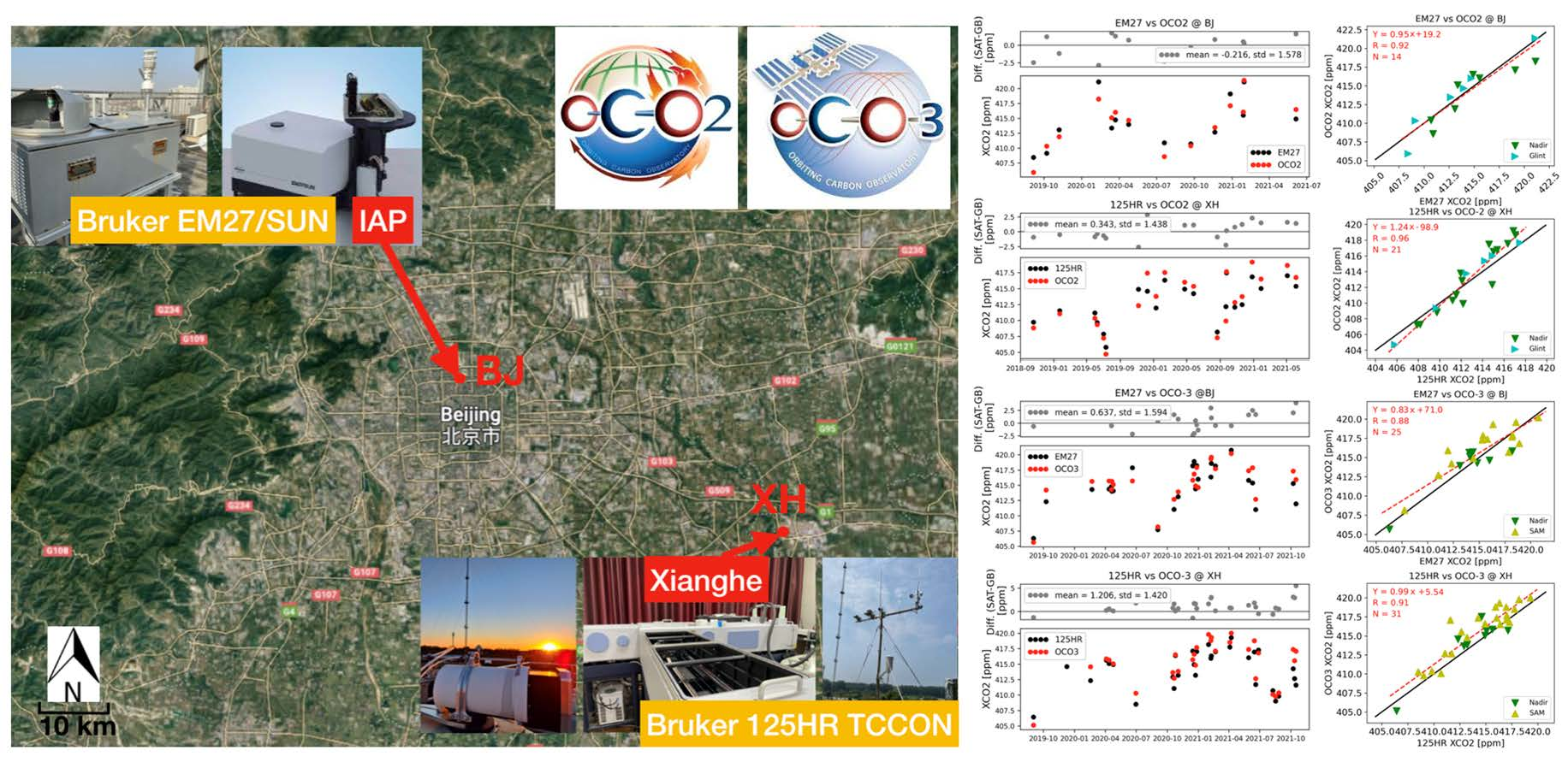
2.1. Data

The ground-based FTIR XCO

_{2}

measurements are operated in Xianghe (39.75

^{\circ}

N, 116.96

^{\circ}

E), which is about 50 km southeast of Beijing, and are affiliated with TCCON, (Figure 1). More detail about the Xianghe FTIR site can be found in Yang et al., (2020) [24]. The spectrum is recorded by 2 scans with the spectral resolution of 0.02 cm

^{- 1}

. The GGG2020 retrieval code, updated from the previous version GGG2014 [28], is used to derive XCO

_{2}

from the observed solar near-infrared (NIR) absorption spectra. The GGG2020 code includes software to convert the interferogram to spectra with the DC correction, a non-linear least-squares fitting algorithm (GFIT), and a post-correction to scale XCO

_{2}

to the WMO standards [19]. The XCO

_{2}

is derived from the CO

_{2}

(

T C_{C O_{2}}

) and O

_{2}

(

T C_{O_{2}}

) retrieved total columns

X C O_{2} = 0.2095 \times \frac{T C_{C O_{2}}}{T C_{O_{2}}} .

(1)

The retrieval windows of CO

_{2}

and O

_{2}

are listed in Table 1. The surface temperature, pressure, and humidity come from the local auto-weather station. The meteorological profiles (H

_{2}

O, T and P) and CO

_{2}

a priori profile are derived from the 3-hourly Goddard Earth Observing System Model, Forward Processing for Instrument Teams (GEOS FP-IT model; https://gmao.gsfc.nasa.gov/GMAO_products/GEOS-IT/, accessed on 30 June 2022). The FTIR XCO

_{2}

measurements in Xianghe are publicly available in https://tccondata.org/, accessed on 30 June 2022.

The portable Bruker EM27/SUN (SN095) instrument is operated on the roof of the IAP (39.98

^{\circ}

N, 116.39

^{\circ}

E), which is located in the center of the city (Figure 1). The measurement setup follows the COCCON. The spectrum is recorded by 10 scans with a spectral resolution of 0.5 cm

^{- 1}

. The EM27/SUN spectra are tested with two retrieval codes: GGG2020 and PROFFAST v1.0. Compared to the GGG2020, the same O

_{2}

retrieval window is used in the PROFFAST v1.0, while the CO

_{2}

retrieval window used in the PROFFAST v1.0 is slightly wider (see Table 1). PROFFAST v1.0 also includes software to convert interferogram to spectra with the DC correction (preprocess) and a non-linear least squares fitting algorithm (inverse). The GEOS FP-IT model data are used for the meteorological and CO

_{2}

a priori profiles. To speed up, the PROFFAST v1.0 uses the meteorological and CO

_{2}

a priori profiles on every measurement day to generate a look-up absorption cross sections table (pcxs) [20]. To reduce the systematic uncertainty, the PROFFAST v1.0 code applies a post-processing to scale the PROFFAST v1.0 retrievals to the TCCON measurements [26].

The lite_v10_FP version of OCO-2 and the lite_v10.4_FP version of the OCO-3 satellite XCO

_{2}

measurements are used in this study. The satellite data are downloaded from https://disc.gsfc.nasa.gov/, accessed on 30 June 2022. The XCO

_{2}

product is retrieved from the O

_{2}

band 0.76

μ

m, the weak CO

_{2}

band at 1.61

μ

m, and the strong CO

_{2}

band at 2.06

μ

m [29]. Both OCO-2 and OCO-3 XCO

_{2}

products have been bias-corrected against with TCCON measurements when Xianghe was not part of the TCCON network [25,29,30]. The spatial resolutions of the OCO-2 and OCO-3 XCO

_{2}

observations are approximately 1.3 km × 2.2 km and 1.6 km × 2.2 km, respectively. OCO-2 was launched to a sun-synchronous orbit in July 2014, and the overpass time is about 13:30 local time. Two observation modes (nadir and glint) are operated by the OCO-2 satellite above Beijing and Xianghe. OCO-3 was launched to the International Space Station in May 2019, and it maintains an orbit with an average altitude of about 400 km. Note that OCO-3 sampling at a particular location varies across all hours of the day. Two observation modes (nadir and SAM) are operated by the OCO-3 satellite above Beijing and Xianghe. Both OCO-2 and OCO-3 XCO

_{2}

data are filtered out with bad quality filtering (qf = 1). To reduce the sampling error, we selected all the OCO-2/3 satellite XCO

_{2}

measurements within only 50 km around the Beijing and Xianghe sites.

In addition to the ground-based and satellite XCO

_{2}

measurements, the ECMWF ERA5 hourly re-analysis data [31] are used to understand the mean meteorological condition between Beijing and Xianghe. ERA5 provides the atmospheric variables with a 0.25

^{\circ}

× 0.25

^{\circ}

horizontal resolution and 137 vertical levels (from surface to ∼80 km).

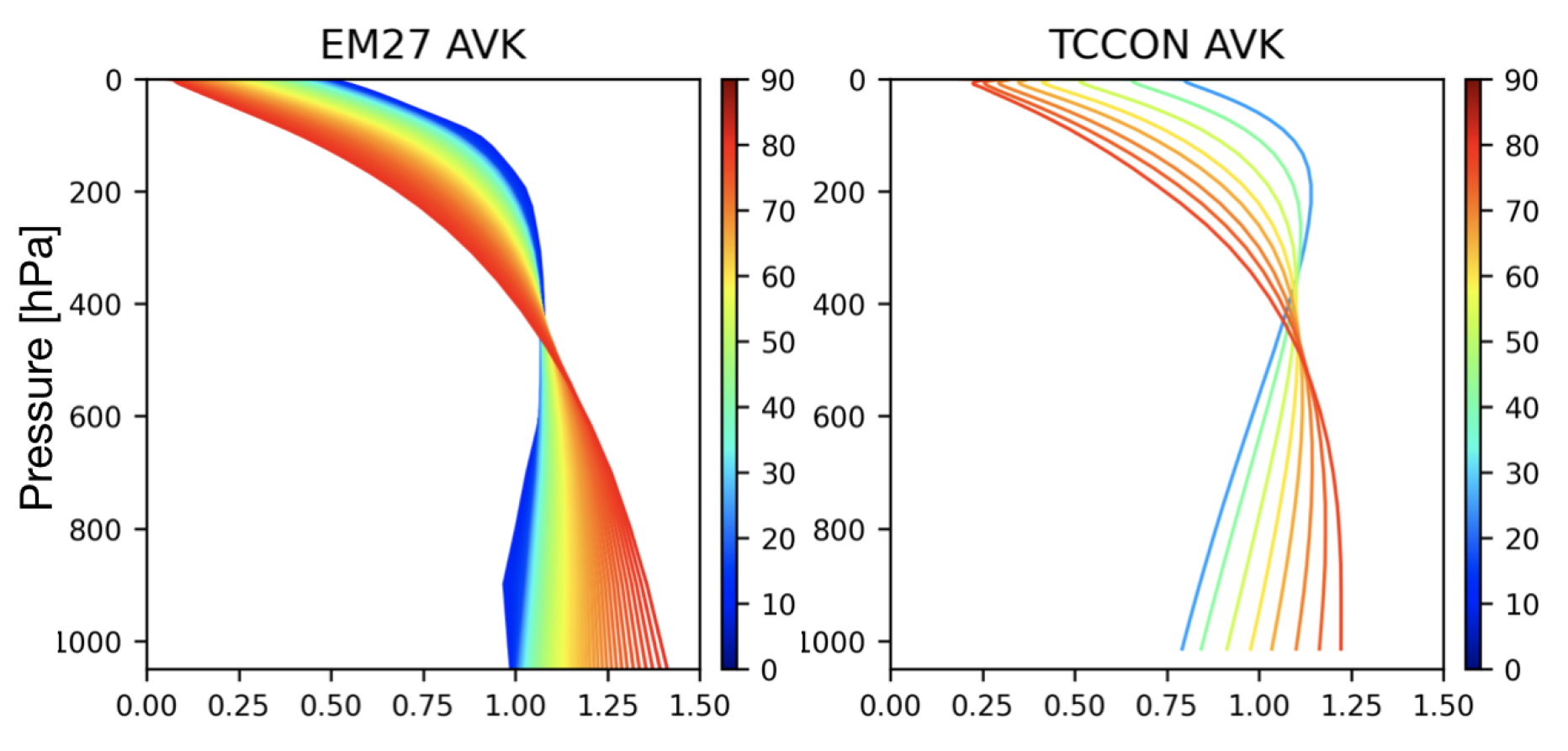
2.2. Method

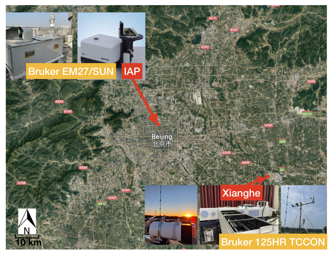
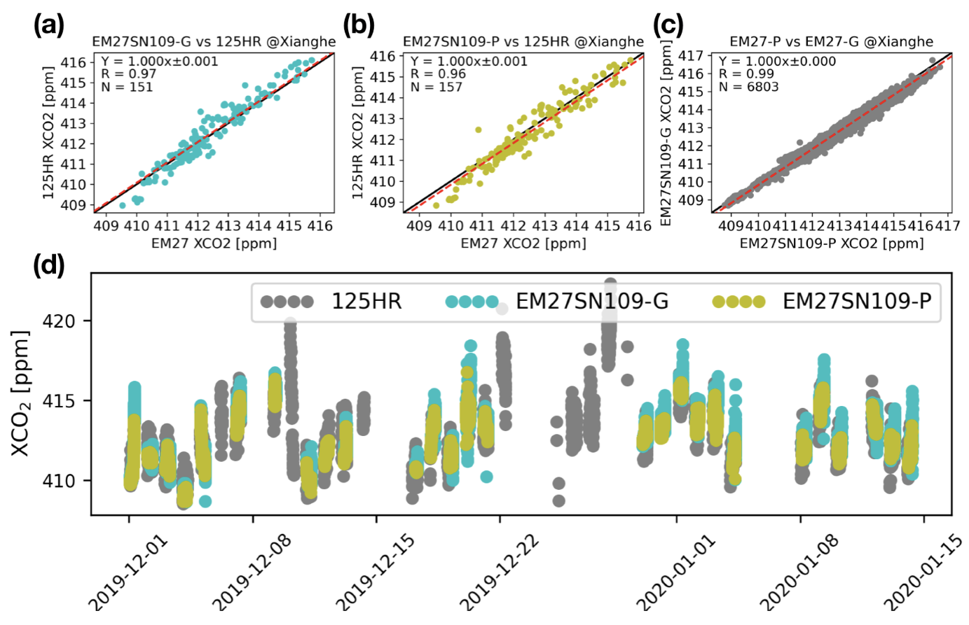
2.2.1. Bruker EM27/SUN in Beijing against Bruker IFS 125HR in Xianghe

To reduce the systematic bias between the EM27/SUN (SN095) measurements in Beijing and Bruker IFS 125HR measurements (TCCON) in Xianghe, we use another EM27/SUN instrument (SN109) as a transfer calibration. First, we operated it close to the EM27/SUN (SN095) in Beijing for about 10 days in 2019 and then moved it close to 125HR TCCON measurements in Xianghe between November 2019 and January 2020. Finally, the EM27/SUN (SN095) retrievals were scaled according to the 125HR measurements.

According to the optimal estimation method [32], the retrieved CO

_{2}

total column can be written as

\begin{matrix} T C_{r} = T C_{a} + \vec{A} \cdot P C_{a i r} ({\vec{x}}_{t} - {\vec{x}}_{a}) + ϵ, \end{matrix}

(2)

where

T C_{r}

and

T C_{a}

are retrieved and a priori total columns, respectively;

{\vec{x}}_{t}

and

{\vec{x}}_{a}

are the true and a priori CO

_{2}

dry air mole fraction profile, respectively. In this study, the same a priori profile is used for the Bruker IFS 125HR measurements (TCCON) in Xianghe and Bruker EM27/SUN (both GGG2020 and PROFFAST v1.0).

P C_{a i r}

is the dry air partial column profile.

\vec{A}

is the column averaging kernel, representing the sensitivity of the retrieved total column to the true CO

_{2}

partial column. Due to the different spectral resolutions, the averaging kernels of Bruker EM27/SUN and Bruker IFS 125HR are slightly different (Figure 2). Note that the averaging kernels derived from GGG2020 and PROFFAST v1.0 are very similar (not shown), which agrees well with previous studies [22,33]. According to the PROFFAST technical note (https://www.imk-asf.kit.edu/downloads/Coccon/Technical%20note%20on%20XCO2%20bias%20in%20current%20P.pdf, accessed on 30 June 2022), we scale the PROFFAST v1.0 retrieved XCO

_{2}

with the following scaling factor f.

\begin{matrix} f = 1.0018 - 0.001 {(S Z A / 90^{\circ})}^{2} . \end{matrix}

(3)

The smoothing error resulting from the different averaging kernels between Bruker IFS 125HR and Bruker EM27/SUN retrievals is

\begin{matrix} T C_{r, H R} - T C_{r, E M} = ({\vec{A}}_{H R} - {\vec{A}}_{E M}) \cdot P C_{a i r} ({\vec{x}}_{t} - {\vec{x}}_{a}) + ϵ, \end{matrix}

(4)

where the subscript

_{H R}

and

_{E M}

donate 125HR and EM27/SUN, respectively. As the

{\vec{x}}_{t}

is unknown, here we use the retrieved TCCON CO

_{2}

in Xianghe as the true status to estimate the uncertainty of

({\vec{x}}_{t} - {\vec{x}}_{a})

. The

({\vec{x}}_{t} - {\vec{x}}_{a})

is about 1%. As a result, the difference caused by different averaging kernels between Bruker IFS 125HR and Bruker EM27/SUN retrievals is estimated to be within 0.008% (∼0.03 ppm). As the smoothing error is relatively small, it is ignored in the following sections.

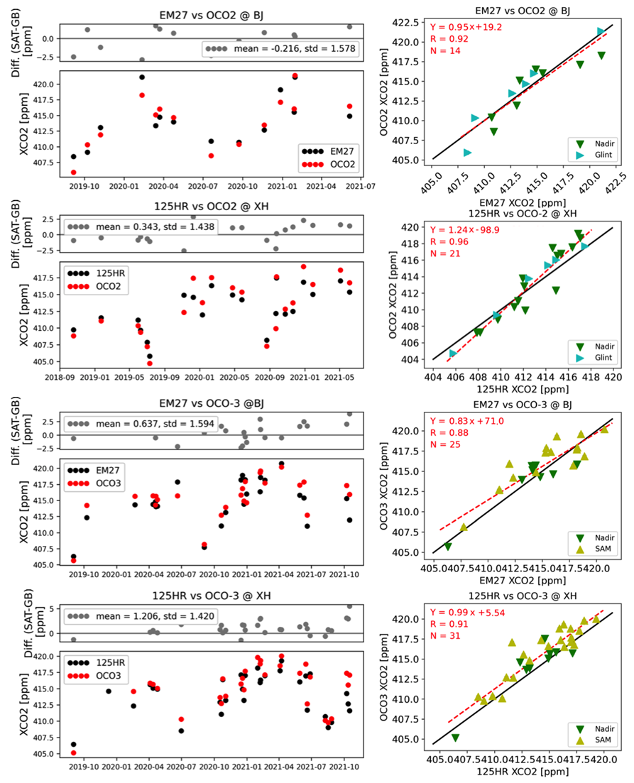
2.2.2. OCO-2/3 Satellite against FTIR Measurements

As mentioned above, the OCO-2/3 satellite measurements within 50 km around Xianghe and Beijing were selected. For each satellite footprint, we chose all the ground-based FTIR measurements within a temporal window of ± 2 h. The criteria (within 50 km and ±2 h) can be motivated because the FTIR signal is typically spread over a 50 km in 2 h with a wind speed of 7 m/s. For each satellite-FTIR data pair, the a priori substitution was performed. In the ACOS version 10, the a priori profile of CO

_{2}

also comes from the GEOS-PFIT model [34]. However, the a priori profiles for each satellite-FTIR data pair can still be different due to their spatial–temporal difference. When comparing the FTIR and satellite retrievals, we use the co-located OCO-2/3 satellite a priori profile for the FTIR retrievals to reduce the impact from their different a priori profiles [35].

\begin{matrix} T C_{r, F} = T C_{a, F} + {\vec{A}}_{F} \cdot P C_{a i r} ({\vec{x}}_{t} - {\vec{x}}_{a, F}) + ϵ, \end{matrix}

(5)

\begin{matrix} T C_{r, F}^{'} = T C_{a, S} + {\vec{A}}_{F} \cdot P C_{a i r} ({\vec{x}}_{t} - {\vec{x}}_{a, S}) + ϵ = T C_{r, F} + ({\vec{A}}_{F} - \vec{I}) \cdot P C_{a i r} ({\vec{x}}_{a, F} - {\vec{x}}_{a, S}), \end{matrix}

(6)

where subscript

_{F}

and

_{S}

represent ground-based FTIR and satellite, respectively. The mean and standard deviation (std) of

T C_{r, F}^{'} - T C_{r, F}

are 0.086 ± 0.109 ppm in Xianghe and 0.092 ± 0.102 ppm in Beijing, respectively. After that, the mean of the corrected FTIR retrievals (

\bar{T C_{r, F}^{'}}

) is used to compare to each satellite retrieval (

T C_{r, S}

). If more than one satellite footprint within 50 km exists around the FTIR site, we use the mean of the satellite retrievals (

\bar{T C_{r, S}}

) to compare to the mean of co-located FTIR measurements. The remaining smoothing error after the priori substitution due to different averaging kernels of ground-based FTIR and OCO-2/3 satellite measurements are estimated to be less than 0.010% (∼0.04 ppm) by using the TCCON retrievals as the true, which is also relative small. Therefore, in this study, the effect from the different averaging kernels between ground-based FTIR and the OCO-2/3 satellite is not taken into account either.

There are mountains with an altitude of over 1 km a.s.l. sited 30 km west and north of Beijing (Figure 1). To reduce the impact of the surface altitude difference between the ground-based FTIR and the satellite measurements, we only select the satellite measurements with a surface pressure (

P_{s}^{S}

) close to that of the co-located FTIR measurement (

P_{s}^{F}

)

| P_{s}^{S} - P_{s}^{F} | < 20 h P a

.

3. Results and Discussion

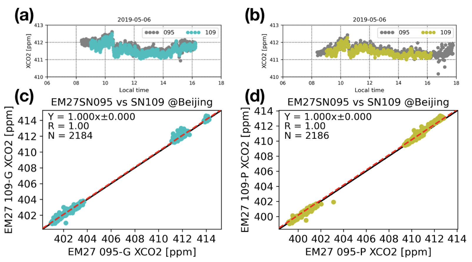
3.1. Scaling Factor of Bruker EM27/SUN Measurements

Two EM27/SUN instruments (SN095 and SN109) were operated together at IAP, Beijing for 10 days between May and September 2019. The relative mean and std bias between the co-located Bruker EM27/SUN SN095 and the SN109 ((SN095-SN109)/SN109 × 100%) were 0.022 ± 0.033% for GGG2020 and 0.039 ± 0.050% for PROFFAST v1.0, respectively. As an example, the EM27/SUN SN095 and SN109 XCO

_{2}

retrievals on 6 May 2019 are shown in Figure 3a,b. We find that the two EM27/SUN instruments have a good agreement. As GGG2020 and PROFFAST v1.0 retrieval codes use different quality control criteria, they do not provide the same valid measurements. For example, there are no GGG2020 retrievals after 16:10 on 6 May 2019, while PROFFAST v1.0 keeps the results after 16:10 for EM27/SUN SN095. Note that the XCO

_{2}

retrievals derived from GGG2020 and PROFFAST v1.0 are slightly different. The reason is probably that a PROFFAST v1.0 airmass correction is made based on the previous TCCON retrievals (GGG2014). Currently, the upgrading of the PROFFAST algorithm from v1.0 to v2.0 is underway, led by Karlsruhe Institute of Technology (Dr. Frank Hase, personal communication), including improvements in the a priori profile, the spectroscopy, and the post corrections. We are looking forward to obtaining a better agreement between EM27/SUN PROFFAST v2.0 and GGG2020 retrievals.

Figure 4 shows the time series of the Bruker 125HR (TCCON) XCO

_{2}

measurements and the Bruker EM27/SUN SN109 measurements retrieved by the GGG2020 and PROFFAST v1.0 codes between December 2019 and January 2020. In total, there are 27 days having both datasets. The Bruker EM27/SUN SN109 XCO

_{2}

measurements retrieved by GGG2020 and PROFFAST v1.0 are very similar, with a good correlation coefficient (R) of 0.99. In addition, both datasets have high correlations against the TCCON measurements with R of 0.97 and 0.96 for GGG2020 and PROFFAST v1.0, respectively. The relative mean and std bias between the co-located Bruker EM27/SUN SN109 and Bruker 125HR ((SN109-125HR)/125HR × 100%) hourly means are −0.018 ± 0.10% for GGG2020 and 0.042 ± 0.11% for PROFFAST v1.0, respectively. Several parameters, e.g., water vapor, temperature, SZA, and SNR, have been further investigated, but we do not find they significantly affect the difference between Bruker EM27/SUN SN109 and Bruker 125HR XCO

_{2}

measurements. Therefore, apart from a constant scaling factor, no further correction is applied to reduce the uncertainty of the Bruker EM27/SUN XCO

_{2}

retrievals.

By applying the EM27/SUN SN109 as the transfer calibration, the EM27/SUN SN095 XCO

_{2}

in Beijing are then scaled with 0.99996 and 0.99920 for GGG2020 and PRFFAST v1.0 retrievals, respectively. As the EM27/SUN GGG2020 retrievals have a slightly better correlation with the 125HR TCCON measurements compared to PROFFAST v1.0 retrievals, we will only show the scaled EM27/SUN SN095 GGG2020 retrievals in the next sections.

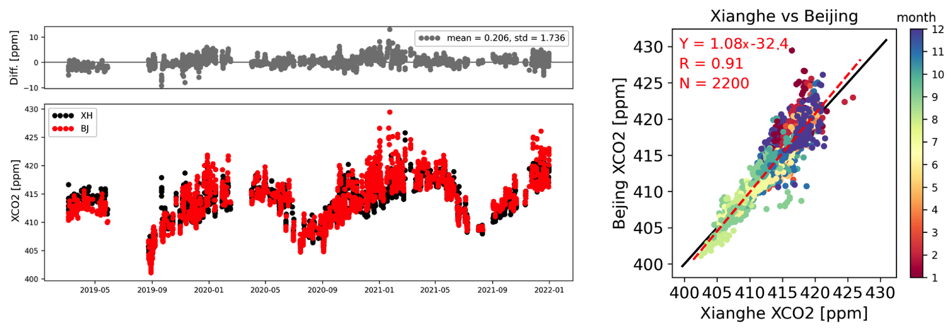
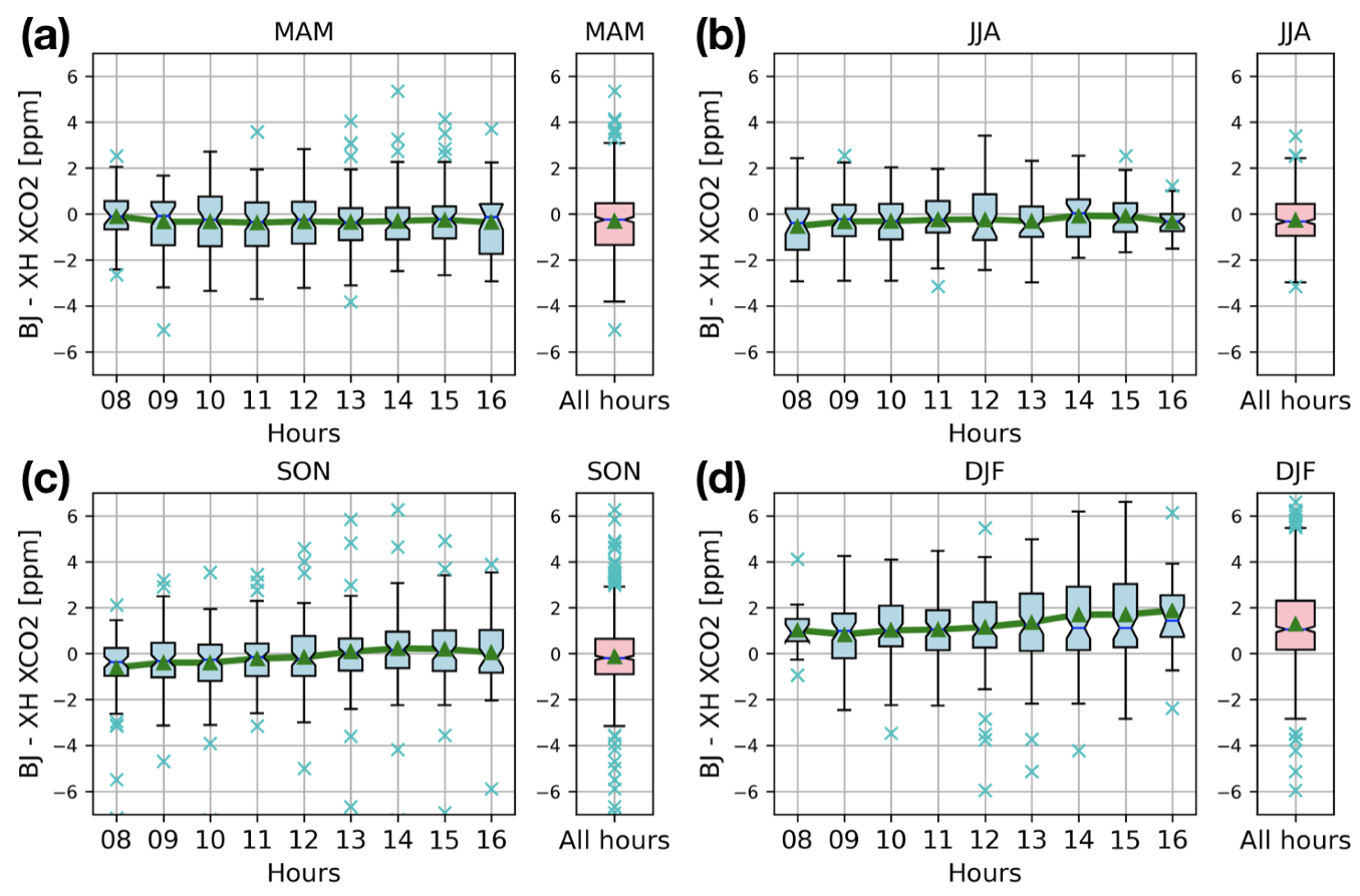
3.2. The Difference between Bruker EM27/SUN Measurements in Beijing and Bruker 125HR Measurements in Xianghe

The time series of the co-located Bruker EM27/SUN XCO

_{2}

hourly means in Beijing and the Bruker 125HR XCO

_{2}

hourly means in Xianghe between March 2019 and December 2021, together with their differences and correlations, are shown in Figure 5. The seasonal cycles of XCO

_{2}

in Beijing and Xianghe are similar, with a maximum in winter and a minimum in summer. The mean and std of the XCO

_{2}

difference (

Δ

XCO

_{2}

) between Beijing and Xianghe (Beijing-Xianghe) are 0.206 ± 1.736 ppm. High correlation (R = 0.91) is found between Beijing and Xianghe. The minimum of

Δ

XCO

_{2}

is about −10 ppm on 21 September 2019, and the maximum of

Δ

XCO

_{2}

is about 13 ppm on 23 January 2021.

The median values of

Δ

XCO

_{2}

are −0.25, −0.33, −0.19, and 1.09 ppm in spring, summer, autumn, and winter, respectively (Figure 6). The mean and median values of

Δ

XCO

_{2}

are close to 0 in spring, summer and autumn, but the XCO

_{2}

in Beijing is larger than that in Xianghe in winter. In spring and summer, there is almost hour-to-hour variation in the

Δ

XCO

_{2}

hourly means. In autumn and winter, the

Δ

XCO

_{2}

hourly means are larger in the afternoon than in the morning. The afternoon–morning differences in XCO

_{2}

(15:00–09:00) are 0.6 ppm in autumn and 0.7 ppm in winter. The large

Δ

XCO

_{2}

in winter observed by two FTIR measurements agrees well with the large

Δ

CO

_{2}

near the surface in winter observed by the Picarro instruments [6]. According to the ERA5 reanalysis data, the boundary layer height (BLH) is about 1 km (about 900 hPa) around local noon in winter. Assuming the CO

_{2}

column difference between Beijing and Xianghe are caused by the CO

_{2}

mole fraction difference in the boundary layer at two places. Consequently, 1.1 ppm difference in XCO

_{2}

leads to about 11 ppm difference in CO

_{2}

mole fraction in the boundary layer.

Meteorological parameters, especially wind speed and wind direction, are crucial to atmospheric transport [36]. Here, we use the ERA5 wind speed and wind direction within 39.5–40.0

^{\circ}

N (latitude) and 116.0–117.0

^{\circ}

E (longitude) at 950 hPa (∼500 m a.s.l) to represent the wind information in the boundary layer in this region. Figure 7a shows the distribution of the wind speed and direction on all FTIR measurement hours. From March to November (spring, summer, and autumn), the dominant wind direction is southwest (b) and from December to February (winter), the dominant wind direction is northwest (c). In all seasons, the wind coming from the east is limited, which accounts for less than 5%. The medians of the

Δ

XCO

_{2}

in eight wind directions are also shown in Figure 7 in all seasons (d), in spring, summer, and autumn (from March to November) (e), and in winter (from December to February) (f). We classify the wind into two categories: wind speed less than 3 m/s (weak wind) and larger than 3 m/s (strong wind). In all seasons (d), the medians of the

Δ

XCO

_{2}

are positive (0.5–1 ppm) with the east, southeast, and south wind directions for both weak and strong wind conditions. For the remaining wind directions, the median of the

Δ

XCO

_{2}

is close to 0 with the weak wind, but it is negative (∼−0.5 ppm) with the strong wind. In spring, summer, and autumn, the medians of the

Δ

XCO

_{2}

in eight directions are slightly less than those in all seasons. In winter, the distribution of

Δ

XCO

_{2}

is quite different. The medians of the

Δ

XCO

_{2}

are about 1–3 ppm with a weak wind speed. The

Δ

XCO

_{2}

medians decrease when increasing the wind speed in west, north, and south directions. The

Δ

XCO

_{2}

medians become close to 0 with the strong wind speed in north, northwest, and west directions. As in other seasons, the

Δ

XCO

_{2}

median is relatively large with the east wind in winter, and the

Δ

XCO

_{2}

median increases when increasing the east wind speed. Tianjin and Tangshan with large CO

_{2}

emissions are both located in the east of Beijing. With a weak east wind, the

Δ

XCO

_{2}

between Beijing and Xianghe is more related to their local emissions difference. With a strong east wind, CO

_{2}

emissions from Tangshan and Tianjin can be transported to Beijing as well. The air mass with a high CO

_{2}

mole fraction can be blocked by the mountain on the west side of Beijing, leading to a larger

Δ

XCO

_{2}

difference between Beijing and Xianghe.

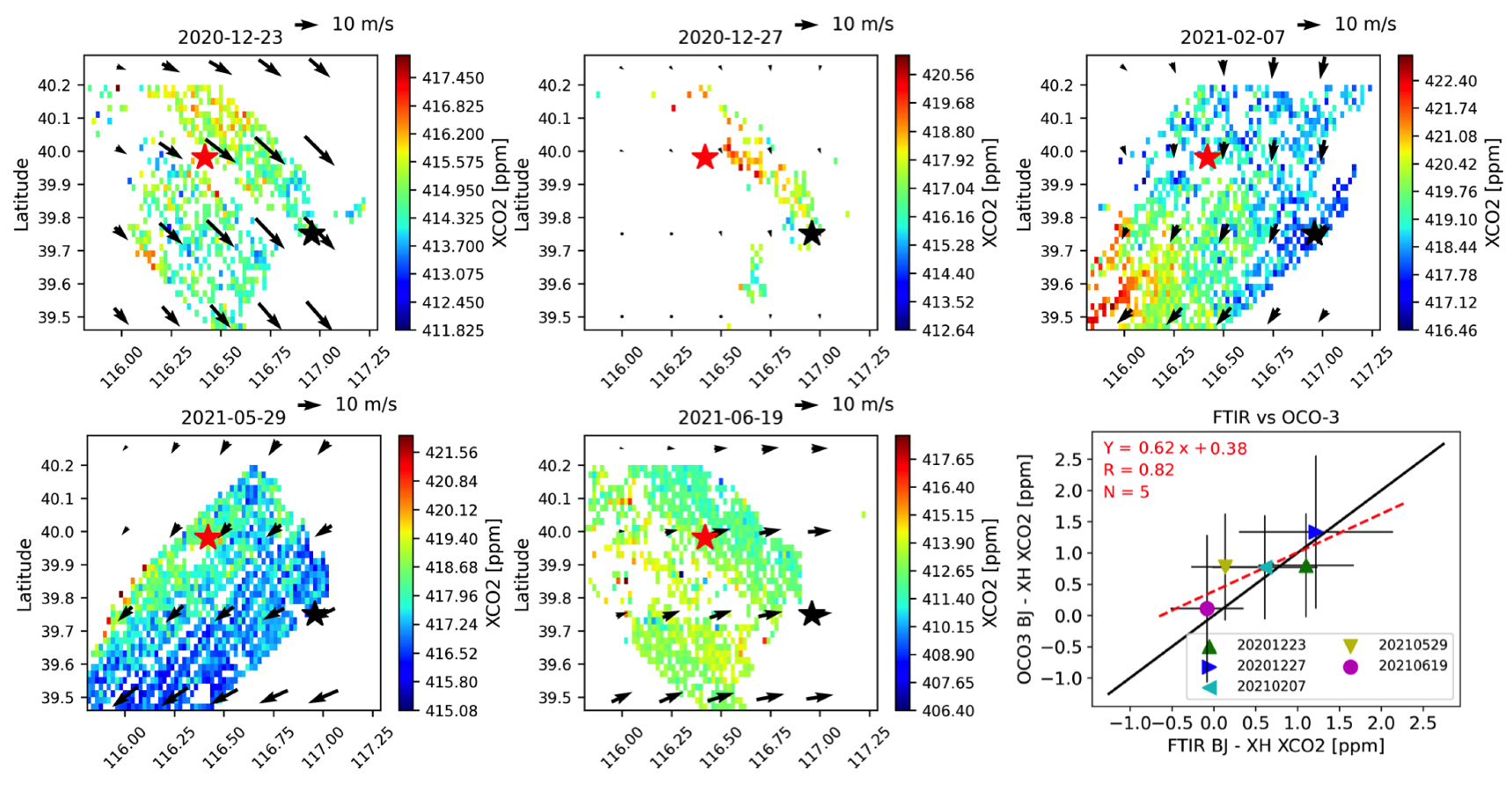
3.3. Validation of OCO-2/3 Satellite Measurements

The time series of the co-located FTIR (EM27/SUN in Beijing and 125HR in Xianghe) and OCO-2/3 XCO

_{2}

measurements, together with their differences and correlations are shown in Figure 8 and Table 2. In general, the OCO-2/3 satellite measurements observe the same seasonal variation of XCO

_{2}

as the one observed by the ground-based FTIR measurements. We find good correlations between OCO-2/3 XCO

_{2}

measurements and the co-located FTIR measurements, with R values ranging from 0.88 to 0.96.

According to the ground-based FTIR measurements, the std of the XCO

_{2}

differences (SAT-GB) for OCO-2 and OCO-3 measurements are similar (about 1.5 ppm). The means of the XCO

_{2}

differences for OCO-2 are relatively small and within 0.35 ppm. Moreover, we do not find a clear difference in the two OCO-2 observation modes (nadir and glint). Regarding the OCO-3 measurements, the mean of the XCO

_{2}

differences for OCO-3 is 0.637 ppm in Beijing and 1.206 ppm in Xianghe, which is larger than the OCO-2. By looking at the different observation modes, the mean of the XCO

_{2}

differences is 0.131 ppm in Beijing and 0.531 ppm in Xianghe for OCO-3 nadir measurements and 0.921 ppm in Beijing and 1.482 ppm in Xianghe for OCO-3 SAM measurements. Both FTIR measurements in Beijing and Xianghe show that the OCO-3 nadir measurements are close to the OCO-2 nadir measurements. However, the OCO-3 SAM measurements are estimated to be 0.9–1.5 ppm overestimated. The OCO-3 SAM mode collects data over 80 × 80 km

^{2}

in 2 min. To further reduce the sampling error, we apply a stricter co-location criterion (within 25 km around the FTIR site and ±1 h FTIR means around each satellite overpass; last row in Table 2). The mean and std of the XCO

_{2}

differences for OCO-3 all data become 0.918 ± 1.512 ppm in Beijing and 0.871 ± 0.617 ppm in Xianghe. It is found that the OCO-3 SAM measurements are still 1.324 ppm and 0.976 ppm larger than the co-located FTIR measurements in Beijing and Xianghe, respectively. The uncertainty of the OCO-3 first public release of OCO-3 Level 2 data (vEarly) SAM XCO

_{2}

have been well estimated with the small area approximation truth proxy training datasets [25], where they found that the root mean square error (RMSE) between the vEarly SAM/target data and the truth proxy (∼1 ppm) is comparable to the RMSE between OCO-2 v9 target mode observations and their truth proxy. However, they pointed out that OCO-3 observations are likely impacted by cloud and aerosol contamination in Southeast Asia, where the quality filtering may not be aggressive enough. In addition, the swath-to-swath bias, which may be driven by the viewing geometries coupled with the polarization angle dependencies in the pointing mirror assembly, may also lead to the uncertainty of OCO-3 SAM observation

Finally, we compare the

Δ

XCO

_{2}

(BJ-XH) observed by the two FTIR measurements and the OCO-3 measurements to understand the spatial gradient observed by the OCO-3 SAM measurements. Figure 9 shows the XCO

_{2}

distribution on the days when the OCO-3 measurements have both measurements around Beijing and Xianghe sites using the strict criteria (within 25 km; ±1 h). The

Δ

XCO

_{2}

observed by the FTIR and OCO-3 measurements have a good agreement, with an R of 0.82 and a slope of 0.619. Although the number of co-located FTIR and OCO-3 SAM measurements is limited (only 5 days), we find that the spatial gradient observed by the OCO-3 SAM measurements is reasonable and promising. The spatial gradient of the XCO

_{2}

observed OCO-2 and OCO-3 nadir and glint measurements have already been applied to calculate the CO

_{2}

flux [14,37,38]. Our result suggests that the spatial gradient of the XCO

_{2}

observed by the OCO-3 SAM mode can be further used for emission estimation in this region despite the systematic bias.

4. Conclusions

Two FTIR instruments (Bruker EM27/SUN SN095 in Beijing and Bruker 125HR in Xianghe) have been recording the solar absorption spectra simultaneously since 2019. Both the 125HR and EM27/SUN spectra are analysed with the latest TCCON retrieval code (GGG2020). The EM27/SUN FTIR XCO

_{2}

measurements in Beijing are scaled with a factor of 0.99996 to get rid of the systematic uncertainty. Based on about 3-years of FTIR measurements, we investigated the differences of XCO

_{2}

between Beijing (urban) and Xianghe (suburb) and showed the FTIR measurements can be used for OCO-2/3 satellite XCO

_{2}

validation.

The mean and std of the

Δ

XCO

_{2}

between Beijing and Xianghe (Beijing–Xianghe) observed by two FTIR instruments were 0.206 ± 1.736 ppm. The

Δ

XCO

_{2}

has a clear seasonal variation. The median values of

Δ

XCO

_{2}

in spring, summer, and autumn are between −0.33 ppm and −0.19 ppm. They are slightly negative, but close to 0. In winter, the median of the

Δ

XCO

_{2}

is 1.09 ppm, which is probably due to that more anthropogenic CO

_{2}

emissions difference between Beijing and Xianghe in winter. Moreover, we found that the

Δ

XCO

_{2}

varies with wind speed and wind direction, especially in winter.

The OCO-2/3 satellite measurements within 50 km around Beijing and Xianghe FTIR sites were selected. Good correlations were found between OCO-2/3 XCO

_{2}

measurements and the co-located FTIR measurements, with R values between 0.88 and 0.96. The mean and std of the XCO

_{2}

differences between OCO-2 and FTIR measurements are −0.216 ± 1.578 ppm in Beijing and −0.343 ± 1.438 ppm in Xianghe. The two observation modes of OCO-2 (nadir and glint) have a similar result. Regarding OCO-3, the mean and std of the XCO

_{2}

differences between OCO-2 and FTIR measurements are 0.637 ± 1.594 ppm in Beijing and 1.206 ± 1.420 ppm in Xianghe. The mean bias of the OCO-3 nadir measurements is similar to the OCO-2 nadir measurements. However, the OCO-3 SAM measurements are overestimated, with the mean bias of 0.9–1.4 ppm. Further investigations are needed to compare the OCO-3 SAM measurements with more ground-based FTIR measurements. Finally, the

Δ

XCO

_{2}

between Beijing and Xianghe observed by two ground-based FTIR measurements were compared to those observed by the OCO-3 SAM measurements, and we found that the OCO-3 SAM measurements can capture the spatial gradient of XCO

_{2}

between urban and suburb well. The FTIR measurements in Beijing and Xianghe suggest that the spatial gradient observed by the OCO-3 SAM mode can be further used for emissions estimation in this region.

Author Contributions

Conceptualization, M.Z. and Z.C.; methodology, M.Z. and Z.C.; writing—original draft preparation, M.Z.; writing—review and editing, Z.C., B.L., Q.N., W.N., Y.Y., K.C., D.Y., T.W., Y.L. and P.W.; visualization, M.Z. All authors have read and agreed to the published version of the manuscript.

Funding

This research was funded by the National Key Research and Development Program of China (2021YFB3901002) and the National Natural Science Foundation of China (41975035).

Data Availability Statement

The OCO-2/3 satellite data are publicly available at https://disc.gsfc.nasa.gov/. The TCCON measurements at Xianghe are publicly available at https://tccondata.org/ (please contact Minqiang Zhou when you use the Xianghe TCCON measurements). The EM27/SUN measurements at Beijing are available upon request to the authors.

Acknowledgments

The authors would like to thank the TCCON and COCCON communities for providing the retrieval codes (GGG2020 and PROFFAST v1.0) and the a priori meteorological data (GEOS FP-IT model simulations), NASA for providing the OCO-2/3 satellite provides. The authors also want to thank Qun Cheng and Qing Yao for their maintenance of TCCON measurements at Xianghe, as well as Yongheng Bi for providing the surface meteorological data at Beijing.

Conflicts of Interest

The authors declare no conflict of interest.

References

IPCC. Climate Change 2013: The Physical Science Basis. Contribution of Working Group I to the Fifth Assessment Report of the Intergovernmental Panel on Climate Change; IPCC: Geneva, Switzerland, 2013. [Google Scholar]
International Energy Agency. World Energy Outlook 2008; OECD Publishing: Paris, France, 2008; p. 576. [Google Scholar] [CrossRef]
Asefi-Najafabady, S.; Rayner, P.J.; Gurney, K.R.; McRobert, A.; Song, Y.; Coltin, K.; Huang, J.; Elvidge, C.; Baugh, K. A multiyear, global gridded fossil fuel CO₂ emission data product: Evaluation and analysis of results. J. Geophys. Res. Atmos. 2014, 119, 10213–10231. [Google Scholar] [CrossRef] [Green Version]
Crippa, M.; Solazzo, E.; Huang, G.; Guizzardi, D.; Koffi, E.; Muntean, M.; Schieberle, C.; Friedrich, R.; Janssens-Maenhout, G. High resolution temporal profiles in the Emissions Database for Global Atmospheric Research. Sci. Data 2020, 7, 121. [Google Scholar] [CrossRef] [PubMed]
Oda, T.; Maksyutov, S.; Andres, R.J. The Open-source Data Inventory for Anthropogenic CO₂, version 2016 (ODIAC2016): A global monthly fossil fuel CO₂ gridded emissions data product for tracer transport simulations and surface flux inversions. Earth Syst. Sci. Data 2018, 10, 87–107. [Google Scholar] [CrossRef] [PubMed] [Green Version]
Yang, Y.; Zhou, M.; Wang, T.; Yao, B.; Han, P.; Ji, D.; Zhou, W.; Sun, Y.; Wang, G.; Wang, P. Spatial and temporal variations of CO₂ mole fractions observed at Beijing, Xianghe, and Xinglong in North China. Atmos. Chem. Phys. 2021, 21, 11741–11757. [Google Scholar] [CrossRef]
Andres, R.J.; Gregg, J.S.; Losey, L.; Marland, G.; Boden, T.A. Monthly, global emissions of carbon dioxide from fossil fuel consumption. Tellus B Chem. Phys. Meteorol. 2011, 63, 309–327. [Google Scholar] [CrossRef] [Green Version]
Baker, D.F.; Law, R.M.; Gurney, K.R.; Rayner, P.; Peylin, P.; Denning, A.S.; Bousquet, P.; Bruhwiler, L.; Chen, Y.H.; Ciais, P.; et al. TransCom 3 inversion intercomparison: Impact of transport model errors on the interannual variability of regional CO₂ fluxes, 1988–2003. Glob. Biogeochem. Cycles 2006, 20. [Google Scholar] [CrossRef] [Green Version]
Nassar, R.; Napier-Linton, L.; Gurney, K.; Andres, R.; Oda, T.; Vogel, F.; Deng, F. Improving the temporal and spatial distribution of co2 emissions from global fossil fuel emission data sets. J. Geophys. Res. Atmos. 2013, 118, 917–933. [Google Scholar] [CrossRef]
Göckede, M.; Michalak, A.M.; Vickers, D.; Turner, D.P.; Law, B.E. Atmospheric inverse modeling to constrain regional-scale CO₂ budgets at high spatial and temporal resolution. J. Geophys. Res. Atmos. 2010, 115. [Google Scholar] [CrossRef] [Green Version]
Kretschmer, R.; Gerbig, C.; Karstens, U.; Koch, F.T. Error characterization of CO₂ vertical mixing in the atmospheric transport model WRF-VPRM. Atmos. Chem. Phys. 2012, 12, 2441–2458. [Google Scholar] [CrossRef] [Green Version]
Keppel-Aleks, G.; Wennberg, P.O.; Schneider, T. Sources of variations in total column carbon dioxide. Atmos. Chem. Phys. 2011, 11, 3581–3593. [Google Scholar] [CrossRef] [Green Version]
Wu, D.; Lin, J.C.; Oda, T.; Kort, E.A. Space-based quantification of per capita CO₂ emissions from cities. Environ. Res. Lett. 2020, 15, 035004. [Google Scholar] [CrossRef]
Nassar, R.; Mastrogiacomo, J.P.; Bateman-Hemphill, W.; McCracken, C.; MacDonald, C.G.; Hill, T.; O’Dell, C.W.; Kiel, M.; Crisp, D. Advances in quantifying power plant CO₂ emissions with OCO-2. Remote Sens. Environ. 2021, 264, 112579. [Google Scholar] [CrossRef]
Kiel, M.; Eldering, A.; Roten, D.D.; Lin, J.C.; Feng, S.; Lei, R.; Lauvaux, T.; Oda, T.; Roehl, C.M.; Blavier, J.F.; et al. Urban-focused satellite CO₂ observations from the Orbiting Carbon Observatory-3: A first look at the Los Angeles megacity. Remote Sens. Environ. 2021, 258, 112314. [Google Scholar] [CrossRef]
Dils, B.; Buchwitz, M.; Reuter, M.; Schneising, O.; Boesch, H.; Parker, R.; Guerlet, S.; Aben, I.; Blumenstock, T.; Burrows, J.P.; et al. The greenhouse gas climate change initiative (GHG-CCI): Comparative validation of GHG-CCI SCIAMACHY/ENVISAT and TANSO-FTS/GOSAT CO₂ and CH4 retrieval algorithm products with measurements from the TCCON. Atmos. Meas. Tech. 2014, 7, 1723–1744. [Google Scholar] [CrossRef] [Green Version]
Zhou, M.; Dils, B.; Wang, P.; Detmers, R.; Yoshida, Y.; O’Dell, C.W.; Feist, D.G.; Velazco, V.A.; Schneider, M.; De Mazière, M. Validation of TANSO-FTS/GOSAT XCO2 and XCH4 glint mode retrievals using TCCON data from near-ocean sites. Atmos. Meas. Tech. 2016, 9, 1415–1430. [Google Scholar] [CrossRef] [Green Version]
Wunch, D.; Wennberg, P.O.; Osterman, G.; Fisher, B.; Naylor, B.; Roehl, C.M.; O’Dell, C.; Mandrake, L.; Viatte, C.; Kiel, M.; et al. Comparisons of the Orbiting Carbon Observatory-2 (OCO-2) XCO2 measurements with TCCON. Atmos. Meas. Tech. 2017, 10, 2209–2238. [Google Scholar] [CrossRef] [Green Version]
Wunch, D.; Toon, G.C.; Blavier, J.F.L.; Washenfelder, R.A.; Notholt, J.; Connor, B.J.; Griffith, D.W.T.; Sherlock, V.; Wennberg, P.O. The Total Carbon Column Observing Network. Philos. Trans. R. Soc. A Math. Phys. Eng. Sci. 2011, 369, 2087–2112. [Google Scholar] [CrossRef] [Green Version]
Frey, M.; Sha, M.K.; Hase, F.; Kiel, M.; Blumenstock, T.; Harig, R.; Surawicz, G.; Deutscher, N.M.; Shiomi, K.; Franklin, J.E.; et al. Building the COllaborative Carbon Column Observing Network (COCCON): Long-term stability and ensemble performance of the EM27/SUN Fourier transform spectrometer. Atmos. Meas. Tech. 2019, 12, 1513–1530. [Google Scholar] [CrossRef] [Green Version]
Messerschmidt, J.; Geibel, M.C.; Blumenstock, T.; Chen, H.; Deutscher, N.M.; Engel, A.; Feist, D.G.; Gerbig, C.; Gisi, M.; Hase, F.; et al. Calibration of TCCON column-averaged CO₂: The first aircraft campaign over European TCCON sites. Atmos. Chem. Phys. 2011, 11, 10765–10777. [Google Scholar] [CrossRef] [Green Version]
Tu, Q.; Hase, F.; Blumenstock, T.; Kivi, R.; Heikkinen, P.; Sha, M.K.; Raffalski, U.; Landgraf, J.; Lorente, A.; Borsdorff, T.; et al. Intercomparison of atmospheric CO₂ and CH4 abundances on regional scales in boreal areas using Copernicus Atmosphere Monitoring Service (CAMS) analysis, COllaborative Carbon Column Observing Network (COCCON) spectrometers, and Sentinel-5 Precursor satellite observations. Atmos. Meas. Tech. 2020, 13, 4751–4771. [Google Scholar] [CrossRef]
Sha, M.K.; De Mazière, M.; Notholt, J.; Blumenstock, T.; Chen, H.; Dehn, A.; Griffith, D.W.T.; Hase, F.; Heikkinen, P.; Hermans, C.; et al. Intercomparison of low- and high-resolution infrared spectrometers for ground-based solar remote sensing measurements of total column concentrations of CO₂, CH₄, and CO. Atmos. Meas. Tech. 2020, 13, 4791–4839. [Google Scholar] [CrossRef]
Yang, Y.; Zhou, M.; Langerock, B.; Sha, M.K.; Hermans, C.; Wang, T.; Ji, D.; Vigouroux, C.; Kumps, N.; Wang, G.; et al. New ground-based Fourier-transform near-infrared solar absorption measurements of XCO2, XCH4 and XCO at Xianghe, China. Earth Syst. Sci. Data 2020, 12, 1679–1696. [Google Scholar] [CrossRef]
Taylor, T.E.; Eldering, A.; Merrelli, A.; Kiel, M.; Somkuti, P.; Cheng, C.; Rosenberg, R.; Fisher, B.; Crisp, D.; Basilio, R.; et al. OCO-3 early mission operations and initial (vEarly) XCO2 and SIF retrievals. Remote Sens. Environ. 2020, 251, 112032. [Google Scholar] [CrossRef]
Sha, M.K.; Langerock, B.; Blavier, J.F.L.; Blumenstock, T.; Borsdorff, T.; Buschmann, M.; Dehn, A.; De Mazière, M.; Deutscher, N.M.; Feist, D.G.; et al. Validation of Methane and Carbon Monoxide from Sentinel-5 Precursor using TCCON and NDACC-IRWG stations. Atmos. Meas. Tech. 2021, 14, 6249–6304. [Google Scholar] [CrossRef]
Cai, Z.; Che, K.; Liu, Y.; Yang, D.; Liu, C.; Yue, X. Decreased Anthropogenic CO₂ Emissions during the COVID-19 Pandemic Estimated from FTS and MAX-DOAS Measurements at Urban Beijing. Remote Sens. 2021, 13, 517. [Google Scholar] [CrossRef]
Wunch, D.; Toon, G.C.; Sherlock, V.; Deutscher, N.M.; Liu, C.; Feist, D.G.; Wennberg, P.O. The Total Carbon Column Observing Network’s GGG2014 Data Version; Technical Report; California Institute of Technology: Pasadena, CA, USA, 2015. [Google Scholar] [CrossRef]
O’Dell, C.W.; Eldering, A.; Wennberg, P.O.; Crisp, D.; Gunson, M.R.; Fisher, B.; Frankenberg, C.; Kiel, M.; Lindqvist, H.; Mandrake, L.; et al. Improved retrievals of carbon dioxide from Orbiting Carbon Observatory-2 with the version 8 ACOS algorithm. Atmos. Meas. Tech. 2018, 11, 6539–6576. [Google Scholar] [CrossRef] [Green Version]
Eldering, A.; Taylor, T.E.; O’Dell, C.W.; Pavlick, R. The OCO-3 mission: Measurement objectives and expected performance based on 1 year of simulated data. Atmos. Meas. Tech. 2019, 12, 2341–2370. [Google Scholar] [CrossRef] [Green Version]
Muñoz Sabater, J. ERA5-Land Hourly Data from 1950 to present. Copernicus Climate Change Service (C3S) Climate Data Store (CDS). Technical Report. 2021. Available online: https://doi.org/10.24381/cds.e2161bac (accessed on 23 February 2020).
Rodgers, C.D. Inverse Methods for Atmospheric Sounding—Theory and Practice, Series on Atmospheric Oceanic and Planetary Physics; World Scientific Publishing Co. Pte. Ltd.: Singapore, 2000; Volume 2, p. 256. [Google Scholar] [CrossRef] [Green Version]
Hedelius, J.K.; Viatte, C.; Wunch, D.; Roehl, C.M.; Toon, G.C.; Chen, J.; Jones, T.; Wofsy, S.C.; Franklin, J.E.; Parker, H.; et al. Assessment of errors and biases in retrievals of X_CO2, X_CH4, X_CO, and X_N2O from a 0.5 cm⁻¹ resolution solar-viewing spectrometer. Atmos. Meas. Tech. 2016, 9, 3527–3546. [Google Scholar] [CrossRef] [Green Version]
Taylor, T.E.; O’Dell, C.W.; Crisp, D.; Kuze, A.; Lindqvist, H.; Wennberg, P.O.; Chatterjee, A.; Gunson, M.; Eldering, A.; Fisher, B.; et al. An 11-year record of XCO₂ estimates derived from GOSAT measurements using the NASA ACOS version 9 retrieval algorithm. Earth Syst. Sci. Data 2022, 14, 325–360. [Google Scholar] [CrossRef]
Rodgers, C.D.; Connor, B.J. Intercomparison of remote sounding instruments. J. Geophys. Res. 2003, 108, 46–48. [Google Scholar] [CrossRef] [Green Version]
Metya, A.; Datye, A.; Chakraborty, S.; Tiwari, Y.K.; Sarma, D.; Bora, A.; Gogoi, N. Diurnal and seasonal variability of CO₂ and CH₄ concentration in a semi-urban environment of western India. Sci. Rep. 2021, 11, 2931. [Google Scholar] [CrossRef] [PubMed]
Zheng, T.; Nassar, R.; Baxter, M. Estimating power plant CO₂ emission using OCO-2 XCO2 and high resolution WRF-Chem simulations. Environ. Res. Lett. 2019, 14, 085001. [Google Scholar] [CrossRef]
Zheng, B.; Chevallier, F.; Ciais, P.; Broquet, G.; Wang, Y.; Lian, J.; Zhao, Y. Observing carbon dioxide emissions over China’s cities and industrial areas with the Orbiting Carbon Observatory-2. Atmos. Chem. Phys. 2020, 20, 8501–8510. [Google Scholar] [CrossRef]

Figure 1. The location of the Bruker EM27/SUN measurements in Beijing (urban) and the Bruker IFS 125HR measurements in Xianghe (suburb). The background map is from Google Maps with the name (English and Chinese) of Beijing remarked (https://www.google.com/maps, accessed on 30 June 2022).

Figure 2. The column averaging kernels of Bruker EM27/SUN (left) and Bruker IFS 125HR (right) CO

_{2}

retrievals varying with the solar zenith angle, which are both analysed by the GGG2020 code.

Figure 2. The column averaging kernels of Bruker EM27/SUN (left) and Bruker IFS 125HR (right) CO

_{2}

retrievals varying with the solar zenith angle, which are both analysed by the GGG2020 code.

Figure 3. The EM27/SUN SN095 and SN109 XCO

_{2}

measurements retrieved by GGG2020 (a) and PRFFAST v1.0 (b) on 6 May 2019, together with their correlation plots on all 10 measurement days using GGG2020 (c) and PRFFAST v1.0 (d). The red dashed line is the linear fitting (

y = a x

). R is the Pearson correlation coefficient. N is the number of co-located data.

Figure 3. The EM27/SUN SN095 and SN109 XCO

_{2}

measurements retrieved by GGG2020 (a) and PRFFAST v1.0 (b) on 6 May 2019, together with their correlation plots on all 10 measurement days using GGG2020 (c) and PRFFAST v1.0 (d). The red dashed line is the linear fitting (

y = a x

). R is the Pearson correlation coefficient. N is the number of co-located data.

Figure 4. The scatter plots between the Bruker 125HR (TCCON) and the Bruker EM27/SUN SN109 co-located XCO

_{2}

hourly means retrieved by the GGG2020 code (a) and by the PROFFAST code (b) in Xianghe. The scatter plots between the Bruker EM27/SUN SN109 individual XCO

_{2}

retrieved by the GGG2020 code and by the PROFFAST code (c). The red dashed line is the linear fitting (

y = a x

). R is the Pearson correlation coefficient. N is the number of co-located data. The time series of the Bruker 125HR (TCCON) XCO

_{2}

measurements and the Bruker EM27/SUN SN109 measurements retrieved by the GGG2020 and PROFFAST v1.0 codes between December 2019 and January 2020 (d).

Figure 4. The scatter plots between the Bruker 125HR (TCCON) and the Bruker EM27/SUN SN109 co-located XCO

_{2}

hourly means retrieved by the GGG2020 code (a) and by the PROFFAST code (b) in Xianghe. The scatter plots between the Bruker EM27/SUN SN109 individual XCO

_{2}

retrieved by the GGG2020 code and by the PROFFAST code (c). The red dashed line is the linear fitting (

y = a x

). R is the Pearson correlation coefficient. N is the number of co-located data. The time series of the Bruker 125HR (TCCON) XCO

_{2}

measurements and the Bruker EM27/SUN SN109 measurements retrieved by the GGG2020 and PROFFAST v1.0 codes between December 2019 and January 2020 (d).

Figure 5. Left panels: the time series of the co-located EM27/SUN SN095 XCO

_{2}

hourly means in Beijing (red) and 125 HR XCO

_{2}

hourly means in Xianghe (black), together with their absolute difference (BJ–XH). Right panel: the scatter plots of the co-located EM27/SUN SN095 and 125 HR XCO

_{2}

hourly means. The red dashed line is the linear fitting (

y = a x

). R is the Pearson correlation coefficient. N is the number of co-located data. The dots are coloured with the measurement months.

Figure 5. Left panels: the time series of the co-located EM27/SUN SN095 XCO

_{2}

hourly means in Beijing (red) and 125 HR XCO

_{2}

hourly means in Xianghe (black), together with their absolute difference (BJ–XH). Right panel: the scatter plots of the co-located EM27/SUN SN095 and 125 HR XCO

_{2}

hourly means. The red dashed line is the linear fitting (

y = a x

). R is the Pearson correlation coefficient. N is the number of co-located data. The dots are coloured with the measurement months.

Figure 6. Box plots of the

Δ

XCO

_{2}

(BJ-XH) observed by two FTIR measurements in each hour and in four seasons ((a) MAM: spring; (b) JJA: summer; (c) SON: autumn; (d) DJF: winter). Each box plot shows the values of relative difference for the maximum (upper solid line), 75th percentile (top of box), median (line through middle of box), mean (green triangle), 25th percentile (bottom of box), and minimum (bottom of solid line) of the distribution. The blue crosses are the outliers.

Figure 6. Box plots of the

Δ

XCO

_{2}

(BJ-XH) observed by two FTIR measurements in each hour and in four seasons ((a) MAM: spring; (b) JJA: summer; (c) SON: autumn; (d) DJF: winter). Each box plot shows the values of relative difference for the maximum (upper solid line), 75th percentile (top of box), median (line through middle of box), mean (green triangle), 25th percentile (bottom of box), and minimum (bottom of solid line) of the distribution. The blue crosses are the outliers.

Figure 7. The wind rose plot of the regional mean wind speed and wind direction within 39.5–40.0

^{\circ}

(latitude) and 116.0–117.0

^{\circ}

(longitude) at 950 hPa derived from the ERA5 reanalysis data on all the FTIR measurement hours (a); in spring, summer, and autumn (March–November (b)); and in winter (DJF (c)). The medians of the

Δ

XCO

_{2}

at eight wind directions in all seasons (d); in spring, summer, and autumn (March–November (e)); and in winter (DJF; (f)). Here, we define weak wind and strong wind with a wind speed of <3 m/s and >3 m/s, respectively.

Figure 7. The wind rose plot of the regional mean wind speed and wind direction within 39.5–40.0

^{\circ}

(latitude) and 116.0–117.0

^{\circ}

(longitude) at 950 hPa derived from the ERA5 reanalysis data on all the FTIR measurement hours (a); in spring, summer, and autumn (March–November (b)); and in winter (DJF (c)). The medians of the

Δ

XCO

_{2}

at eight wind directions in all seasons (d); in spring, summer, and autumn (March–November (e)); and in winter (DJF; (f)). Here, we define weak wind and strong wind with a wind speed of <3 m/s and >3 m/s, respectively.

Figure 8. The time series and correlation plots of the co-located FTIR and OCO-2/3 satellite measurements. From top to bottom: EM27/SUN against OCO-2 in Beijing; 125HR against OCO-2 in Xianghe, EM27/SUN against OCO-3 in Beijing; and 125HR against OCO-3 in Xianghe. OCO-2 provides nadir and glint measurements, and OCO-3 provides nadir and snapshot area mode (SAM) measurements over Beijing and Xianghe.

Figure 9. The spatial distribution of XCO

_{2}

observed by the OCO-3 SAM measurements, together with the wind at 950 hPa, on 23 December 2020, 27 December 2020, 7 February 2021, 29 May 2021, and 19 June 2021 over Beijing and Xianghe FTIR sites, remarked as the red and black stars, respectively. The right bottom panel is the scatter plot between the

Δ

XCO

_{2}

(BJ-XH) observed by FTIR measurements and

Δ

XCO

_{2}

observed by the OCO-3 SAM measurements. The error bar is the uncertainty of the FTIR and OCO-3 measurements.

Figure 9. The spatial distribution of XCO

_{2}

observed by the OCO-3 SAM measurements, together with the wind at 950 hPa, on 23 December 2020, 27 December 2020, 7 February 2021, 29 May 2021, and 19 June 2021 over Beijing and Xianghe FTIR sites, remarked as the red and black stars, respectively. The right bottom panel is the scatter plot between the

Δ

XCO

_{2}

(BJ-XH) observed by FTIR measurements and

Δ

XCO

_{2}

observed by the OCO-3 SAM measurements. The error bar is the uncertainty of the FTIR and OCO-3 measurements.

Table 1. The instrumental characters of Bruker IFS 125HR in Xianghe and Bruker EM27/SUN in Beijing, together with their XCO

_{2}

retrieval settings.

Table 1. The instrumental characters of Bruker IFS 125HR in Xianghe and Bruker EM27/SUN in Beijing, together with their XCO

_{2}

retrieval settings.

Instrument	Bruker IFS 125HR	Bruker EM27/SUN
retrieval code	GGG2020	GGG2020	PROFFAST v1.0
Spectral resolution (cm $^{- 1}$ )	0.02	0.5
CO $_{2}$ retrieval window (cm $^{- 1}$ )	6180–6260, 6297–6382	6180–6260, 6297–6382	6173–6390
O $_{2}$ retrieval window (cm $^{- 1}$ )	7765–8005
A priori profile	GEOS FP-IT model

Table 2. The mean and std of the difference between co-located ground-based FTIR and OCO-2/3 satellite measurements (SAT-GB) for all satellite observation modes and for each individual mode.

		Beijing EM27	Xianghe 125HR
	All	−0.216 ± 1.578 ppm	0.343 ± 1.438 ppm
OCO-2 (within 50 km; ±2 h)	Nadir	−0.302 ± 1.660 ppm	0.326 ± 1.609 ppm
	Glint	0.009 ± 1.293 ppm	0.384 ± 0.870 ppm
	All	0.637 ± 1.594 ppm	1.206 ± 1.420 ppm
OCO-3 (within 50 km; ±2 h)	Nadir	0.131 ± 1.328 ppm	0.531 ± 1.335 ppm
	SAM	0.921 ± 1.660 ppm	1.482 ± 1.360 ppm
	All	0.918 ± 1.512 ppm	0.871 ± 0.617 ppm
OCO-3 (within 25 km; ±1 h)	Nadir	−0.369 ± 1.723 ppm	0.453 ± 0.418 ppm
	SAM	1.324 ± 1.153 ppm	0.976 ± 0.644 ppm

Publisher’s Note: MDPI stays neutral with regard to jurisdictional claims in published maps and institutional affiliations.

© 2022 by the authors. Licensee MDPI, Basel, Switzerland. This article is an open access article distributed under the terms and conditions of the Creative Commons Attribution (CC BY) license (https://creativecommons.org/licenses/by/4.0/).

Share and Cite

MDPI and ACS Style

Zhou, M.; Ni, Q.; Cai, Z.; Langerock, B.; Nan, W.; Yang, Y.; Che, K.; Yang, D.; Wang, T.; Liu, Y.; et al. CO₂ in Beijing and Xianghe Observed by Ground-Based FTIR Column Measurements and Validation to OCO-2/3 Satellite Observations. Remote Sens. 2022, 14, 3769. https://doi.org/10.3390/rs14153769

AMA Style

Zhou M, Ni Q, Cai Z, Langerock B, Nan W, Yang Y, Che K, Yang D, Wang T, Liu Y, et al. CO₂ in Beijing and Xianghe Observed by Ground-Based FTIR Column Measurements and Validation to OCO-2/3 Satellite Observations. Remote Sensing. 2022; 14(15):3769. https://doi.org/10.3390/rs14153769

Chicago/Turabian Style

Zhou, Minqiang, Qichen Ni, Zhaonan Cai, Bavo Langerock, Weidong Nan, Yang Yang, Ke Che, Dongxu Yang, Ting Wang, Yi Liu, and et al. 2022. "CO₂ in Beijing and Xianghe Observed by Ground-Based FTIR Column Measurements and Validation to OCO-2/3 Satellite Observations" Remote Sensing 14, no. 15: 3769. https://doi.org/10.3390/rs14153769

APA Style

Zhou, M., Ni, Q., Cai, Z., Langerock, B., Nan, W., Yang, Y., Che, K., Yang, D., Wang, T., Liu, Y., & Wang, P. (2022). CO₂ in Beijing and Xianghe Observed by Ground-Based FTIR Column Measurements and Validation to OCO-2/3 Satellite Observations. Remote Sensing, 14(15), 3769. https://doi.org/10.3390/rs14153769

Note that from the first issue of 2016, this journal uses article numbers instead of page numbers. See further details here.

Article Menu