Comparative Evaluation of a Newly Developed Trunk-Based Tree Detection/Localization Strategy on Leaf-Off LiDAR Point Clouds with Varying Characteristics

Abstract

LiDAR data acquired by various platforms provide unprecedented data for forest inventory and management. Among its applications, individual tree detection and segmentation are critical and prerequisite steps for deriving forest structural metrics, especially at the stand level. Although there are various tree detection and localization approaches, a comparative analysis of their performance on LiDAR data with different characteristics remains to be explored. In this study, a new trunk-based tree detection and localization approach (namely, height-difference-based) is proposed and compared to two state-of-the-art strategies—DBSCAN-based and height/density-based approaches. Leaf-off LiDAR data from two unmanned aerial vehicles (UAVs) and Geiger mode system with different point densities, geometric accuracies, and environmental complexities were used to evaluate the performance of these approaches in a forest plantation. The results from the UAV datasets suggest that DBSCAN-based and height/density-based approaches perform well in tree detection (F1 score > 0.99) and localization (with an accuracy of 0.1 m for point clouds with high geometric accuracy) after fine-tuning the model thresholds; however, the processing time of the latter is much shorter. Even though our new height-difference-based approach introduces more false positives, it obtains a high tree detection rate from UAV datasets without fine-tuning model thresholds. However, due to the limitations of the algorithm, the tree localization accuracy is worse than that of the other two approaches. On the other hand, the results from the Geiger mode dataset with low point density show that the performance of all approaches dramatically deteriorates. Among them, the proposed height-difference-based approach results in the greatest number of true positives and highest F1 score, making it the most suitable approach for low-density point clouds without the need for parameter/threshold fine-tuning.

1. Introduction

Forest ecosystems are of ecological and economic importance in providing various ecosystem services such as carbon sequestration and timber and fiber production [1,2]. To ensure appropriate management, an accurate and efficient forest inventory is critical [3]. Traditional forest inventory is carried out through intensive field measurements. Forested lands usually cover large areas that contain too many trees to feasibly count in a costly and timely manner. To address this issue, a small subset of trees are selected for field measurements to help extrapolate the attributes for the entire region [4]. In recent decades, with rapid advancements in sensors and platforms, remote sensing has emerged as a useful alternative to traditional forest inventory, requiring far less tedious field work. For example, satellite imagery has already been adopted for various applications in forest mapping, including forest/non-forest area detection, composition and structure measurement, biomass prediction, and impacts assessment for forest fires [5,6,7,8]. In addition, imagery with a higher geometric resolution, acquired by manned aerial systems and unmanned aerial vehicles (UAVs), has been adopted for growth monitoring, leaf area index (LAI) evaluation, and canopy cover prediction [9,10,11]. One of the major limitations of image-based forest inventory is that while the data provide plenty of planimetric information about the top layer, information related to the forest vertical structure is inadequate. As a result, deriving tree-level inventory metrics such as tree height, crown depth, and diameter at breast height (DBH) from imagery is quite challenging [12].

At present, an increasing number of researchers are adopting LiDAR—an active remote sensing technology that directly derives 3D coordinates from laser pulses—in forest inventory. LiDAR units onboard manned aerial systems (i.e., airborne LiDAR) are the most popular options, as they can efficiently cover a large area with a relatively fine spatial resolution [13]. Most of these units are based on conventional linear LiDAR systems. The acquired data have been used to derive various metrics for forest characteristics, including LAI [14,15], terrain model [16,17], tree species [18], and stem volume and spatial distribution [19,20]. Data collected by airborne linear LiDAR suffer from an insufficient mapping of under canopy structure due to LiDAR’s limited viewing angles. To resolve this issue, full-waveform LiDAR that records the entire return of the reflected laser pulse is used to gain more information related to the vertical structure of trees [21,22]. However, the accuracy of full-waveform LiDAR is usually low due to its large footprint. Moreover, complex processing is required to extract useful information from a substantial amount of data.

Modern single photon LiDAR (SPL) provides another alternative. Using Geiger-mode LiDAR as an example, with low power signal emission and a high-sensitivity receiver, a 2D image array records reflected energy at the photon level. This allows for the Geiger-mode LiDAR to operate at higher altitude and faster flying speed while capturing fine details of the area of interest (i.e., higher point density) compared to traditional linear LiDAR. Several studies have been conducted, extracting individual trees and deriving vertical structure information using single photon LiDAR [23,24]. Regardless of the LiDAR technology used, the acquirement of data through airborne LiDAR is constrained by cost and weather conditions.

While airborne LiDAR is suitable for regional scale applications, UAV LiDAR provides a promising tool for mapping a relatively small forest area with high spatial and temporal resolution owing to its close sensor-to-object distance and ease of operation. Despite its limited spatial coverage, a UAV-LiDAR system allows for fine details of internal forest structure to be captured, along with tree canopy. Accordingly, UAV LiDAR is widely used for fine-scale forest inventory including individual tree extraction, tree height evaluation, and DBH estimation [25,26,27,28].

Compared to the above modalities, proximal LiDAR—e.g., terrestrial laser scanning (TLS) and backpack LiDAR—provides the highest level of details of the internal forest structure. Using TLS data, accurate single tree modeling is possible for estimating metrics such as DBH, tree height, and stem volume [29,30,31]. However, it is highly time-consuming to collect overlapping TLS scans and register them together. With similar sensor-to-object distances as TLS, backpack LiDAR systems provide an efficient alternative for capturing detailed vertical structure information [32,33]. However, intermittent access to the global navigation satellite system (GNSS) signal under the canopy deteriorates the accuracy of the trajectory and, consequently, the geometric quality of the derived point cloud.

Comprehensive studies have been conducted to compare the impact of varying characteristics of LiDAR data from these different modalities on forest inventory [24,25,34,35,36,37,38,39,40,41,42]. The major findings can be summarized as follows:

• Airborne LiDAR systems (ALS) with large spatial coverage are suitable for regional canopy height model (CHM) generation, while small foot-print LiDAR from low altitude flights provides high-resolution data for individual tree isolation;
• UAV and Geiger-mode LiDAR are adequate for individual tree localization and tree height estimation. Although the former has a higher point density and better penetration ability, the latter is capable of deriving accurate point clouds with reasonable resolution over much larger areas;
• Due to the occlusion problem caused by dense canopy, it is recommended to conduct UAV flights under leaf-off conditions to derive digital terrain model (DTM) and timber volume;
• Compared to ALS and UAV LiDAR, Backpack LiDAR can capture a fine level of detail with high precision, allowing for the derivation of forest inventory metrics at the stand level.

Among all forest inventory applications using 3D point clouds, individual tree detection, localization, and segmentation are critical and prerequisite steps for the further derivation of forest structural metrics such as tree height, DBH, canopy cover, and stem volume. Extensive approaches to detecting, localizing, and segmenting individual trees from various forest environments have been proposed. Such approaches can be categorized into two groups: crown-based and trunk-based strategies. Crown-based strategies identify and segment individual tree crowns using LiDAR point clouds related to the forest upper-canopy. This task is mainly conducted in two ways: using rasterized point clouds or original 3D points. The former typically detects trees from a CHM/digital surface model (DSM) in two steps: (i) use the local maximum height as the treetop; (ii) delineate tree crowns as individual trees using different algorithms—e.g., region growing [43], local maximum filtering [44,45], and marker-controlled watershed segmentation [46,47,48]. Instead of using CHM/DSM, Shao et al. [49] developed an approach that relies on a point density model (PDM). They assumed that the center of each individual tree would intercept more LiDAR points than the edges and used a marker-controlled watershed segmentation to delineate individual crowns from PDM. To avoid the artifacts introduced by the interpolation process in CHM/PDM generation, several approaches that directly detect individual trees from original 3D point clouds were proposed. For instance, Li et al. [50] developed a top-down region growing approach that segmented individual trees from the tallest to the shortest. Overall, crown-based strategies could accurately identify large and dominant trees but exhibit poor performance when detecting small trees below the canopy [51].

Trunk-based strategies rely on point clouds that capture tree trunks for detection and localization, followed by a segmentation process based on the identified tree locations. These strategies are usually preferable when adequate point density is present in the understory layer, since trunks are naturally separated from each other while the canopy tends to interlock [51]. Based on the assumption that the intensity values of tree trunks in the LiDAR point cloud are higher than those from smaller branches and foliage, Lu et al. [52] extracted tree trunks and then segmented individual trees by assigning LiDAR points to the tree trunks with the closest planimetric distance. Several approaches adopted the Density Based Spatial Clustering of Applications with Noise (DBSCAN)—a clustering algorithm—for trunk detection [32,53,54,55]. DBSCAN is well-suited to automatic trunk detection as the algorithm does not require the number of clusters (in this case, the number of trees) as an input. Tao et al. [53] adopted DBSCAN on a horizontal slice of normalized LiDAR point cloud at 1.3 m height to perform trunk detection. Then, based on the detected tree trunks, a comparative shortest-path algorithm that follows a bottom-up scheme was developed to assign each LiDAR point to individual trees for segmentation. Given that the input parameters of DBSCAN need to be manually assigned, Fu et al. [55] proposed an improved DBSCAN-based tree detection algorithm. In this approach, a distance distribution matrix was constructed and used to automatically derive the DBSCAN parameters. Once tree trunks were derived, a bottom-up region growing clustering algorithm was used to group point clouds that belong to individual trees. DBSCAN-based approaches have been tested on high-quality data—e.g., TLS [56], backpack LiDAR [32], and below-canopy UAV flights [51,54]—and good results have been achieved. Instead of purely relying on density, Lin et al. [51] proposed an approach based on both elevation information and density by assuming that the higher elevation and/or point density in the understory layer correspond to tree locations. Two-dimensional (2D) cells of the area of interest are created, where the sum of elevations of all points in each cell is evaluated. Then, 2D peak detection is performed to identify the local maxima as the tree location. Finally, segmentation is carried out by assigning each LiDAR point to the tree trunk with the smallest planimetric distance. The authors stated that the height/density-based approach outperforms DBSCAN when dealing with point clouds with relatively sparse density [51].

Although promising results have been achieved through DBSCAN-based and height/density-based approaches, both strategies require threshold fine-tuning for tree detection and localization. Therefore, a more parameter-robust strategy is needed to reduce the amount of manual intervention in forest inventory procedures. Moreover, the abovementioned trunk-based strategies rely on a substantial number of points with high geometric accuracy being detected on tree trunks for accurate tree detection. Their performance under different LiDAR data characteristics (especially point density and geometric accuracy), as well as their environmental complexity, remains to be investigated.

In this study, a height-difference-based tree trunk detection and localization approach (hereafter denoted as the height-difference-based approach) is proposed. This approach is based on the hypothesis that LiDAR points belonging to a tree trunk exhibit large height differences in a local neighborhood. Without relying on LiDAR point density information, the parameters can be defined in a more intuitive way, considering the geometric characteristics of trees (e.g., trunk diameter and average trunk spacing). In this paper, we compare the performance of three trunk-based tree detection and localization approaches including (i) DBSCAN-based approach, (ii) height/density-based approach, and (iii) the proposed height-difference-based approach.

To ensure a fair comparison among different algorithms, a common framework is adopted for LiDAR data preprocessing and understory layer partitioning. Then, the aforementioned three approaches are adopted for individual tree detection and localization, followed by a segmentation process based on trunk location and planimetric distance. UAV LiDAR and Geiger-mode LiDAR are the ideal modalities to acquire finely detail data and derive metrics for individual trees over large areas at a reasonable cost. Therefore, two UAV and one Geiger-mode LiDAR datasets over a plantation area under leaf-off conditions are used to evaluate the performance of the approaches. It is worth mentioning that, for one piece of UAV data, the LiDAR system calibration parameters were out-of-date, resulting in point clouds with low geometric accuracy. To resolve this issue, we also propose a novel system calibration process using tree trunks and ground patches. Lastly, a comparative analysis is performed according to the tree detection and localization accuracy under different scenarios, as well as the execution time. The key contributions of this work can be summarized as follows:

• Propose a new tree detection and localization approach based on the local height differences related to tree trunks;
• Propose a novel system calibration approach for the UAV LiDAR system based on tree trunks and ground patches extracted from a forest dataset;
• Conduct a comparative analysis of three different tree trunk detection/localization strategies—DBSCAN-based approach, height/density-based approach, and height-difference-based approach, while highlighting the main differences;
• Assess the impact of point density, geometric quality, and environmental complexity on the performance of these three approaches, providing recommendations on the selection of appropriate tree detection and localization approaches for leaf-off LiDAR data with different characteristics.

The remainder of the paper is structured as follows: Section 2 describes the study area, utilized LiDAR systems, and characteristics of the acquired datasets. Section 3 introduces the proposed tree detection and segmentation framework, along with the three tree detection and localization approaches, as well as a novel UAV-LiDAR system calibration strategy. Section 4 presents the experimental results, and Section 5 discusses key findings. Finally, Section 6 provides conclusions and recommendations for future work.

2. Data Acquisition Systems and Dataset Description

Three datasets were acquired for this study over a forest plantation under leaf-off conditions using two UAV-based mobile mapping systems and a Geiger-mode LiDAR onboard a manned aircraft. The two UAV systems were developed in-house by the Digital Photogrammetry Research Group at Purdue University. The Geiger-mode LiDAR data were provided by VeriDaaS Corporation (Denver, CO, USA). This section starts by introducing the UAV and Geiger-mode data acquisition systems, followed by a description of the study site and characteristics of the three datasets used in this study.

2.1. Mobile LiDAR Systems

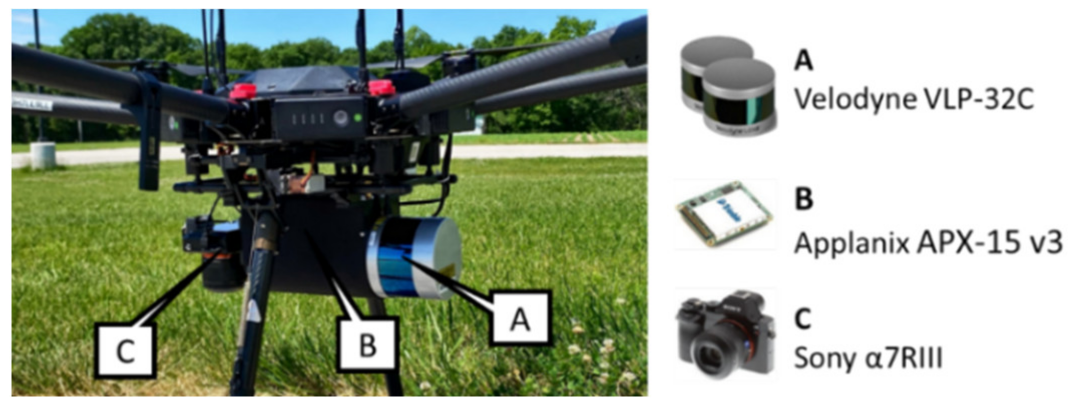
2.1.1. UAV LiDAR Systems

In this study, two in-house developed UAV systems were used—denoted as UAV-1 and UAV-2. The UAV-1 (as shown in Figure 1) payload consists of a Velodyne VLP-32C LiDAR [57] and a Sony α7R III camera. The payload of the UAV-2 is the same as UAV-1 except for its camera, which is a Sony α7R camera. The LiDAR data were directly georeferenced through an Applanix APX15 v3 position and orientation unit with an integrated global navigation satellite system/inertial navigation system (GNSS/INS) [58]. The VLP-32C scanner is a spinning multi-beam LiDAR unit assembled with 32 radially oriented laser rangefinders. Unlike linear LiDAR systems, which have only one laser beam, a multi-beam LiDAR rotates and fires multiple beams in different directions, which mitigate occlusion problems since an object space location can be captured by multiple laser beams at different times. The rotation axes of the LiDAR units on both UAV systems were set to be approximately parallel to the flying direction. To obtain the most accurate point cloud possible, a point is only reconstructed when the laser beam pointing direction is less than ±70° from the nadir. System calibrations of these two UAV systems were conducted using an in situ calibration procedure [59]. The expected accuracy of the acquired point cloud was estimated based on the individual sensor specifications and system calibration accuracy using a LiDAR Error Propagation calculator [60]. At a flying height of 50 m, the calculator suggests that the horizontal/vertical accuracy values are within ±5–6 cm at the nadir position. At the edge of the swath, i.e., ±70° from the nadir, the horizontal/vertical accuracy values would be within ±8–9 cm and ±5–6 cm, respectively.

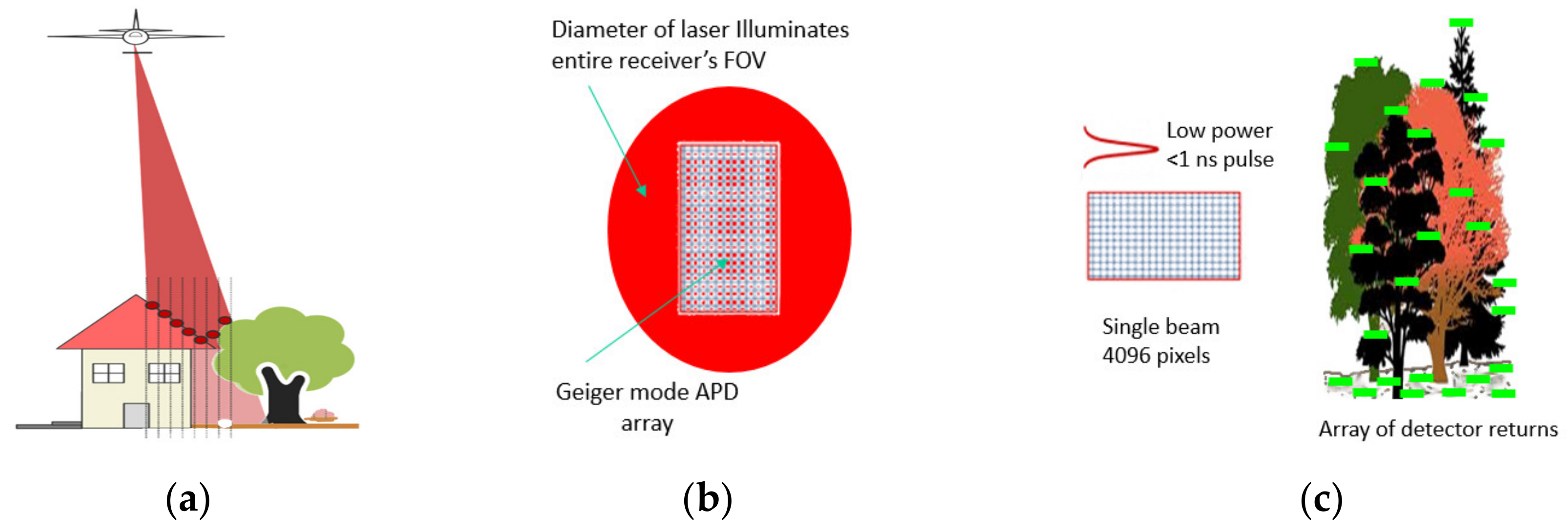
2.1.2. Geiger-Mode LiDAR System

Unlike traditional linear LiDAR, which has high signal emission power and a low-sensitivity receiver, Geiger-mode LiDAR is a relatively new technology that has low signal emission power and a high-sensitivity receiver. The beam divergence of a Geiger-mode LiDAR is large (e.g., a cone) and can illuminate a large area, as shown in Figure 2a. The returning signal covers the entire field of view (FOV) of its 2D receiver, which consists of an array of Geiger-mode Avalanche Photodiode (GmAPD) detectors, as shown in Figure 2b. The GmAPD detectors are designed to be extremely sensitive. Compared to linear LiDAR with a low-sensitivity receiver, which requires hundreds of photons to record a response, the GmAPD detectors record the energy reflected from a single photon [61]; thus, measurements were acquired at a much higher density [62,63] than linear LiDAR systems. The design of the Geiger-mode LiDAR system allows for it to operate at a lower energy, higher altitude, and faster flying speed. In this study, the Geiger mode LiDAR dataset was provided by VeriDaaS Corporation. The VeriDaaS system has an array of 32 by 128 GmAPD detectors, as shown in Figure 2c, which effectively collect 204,800,000 observations per second when using a pulse repetition rate of 50 kHz. The use of a Palmer scanner, together with a 15° scan angle of the laser and scan pattern with a 50% swath overlap, enables multi-view data collection, which can minimize occlusions. This system is directly georeferenced through an Applanix POS AV 610 [64].

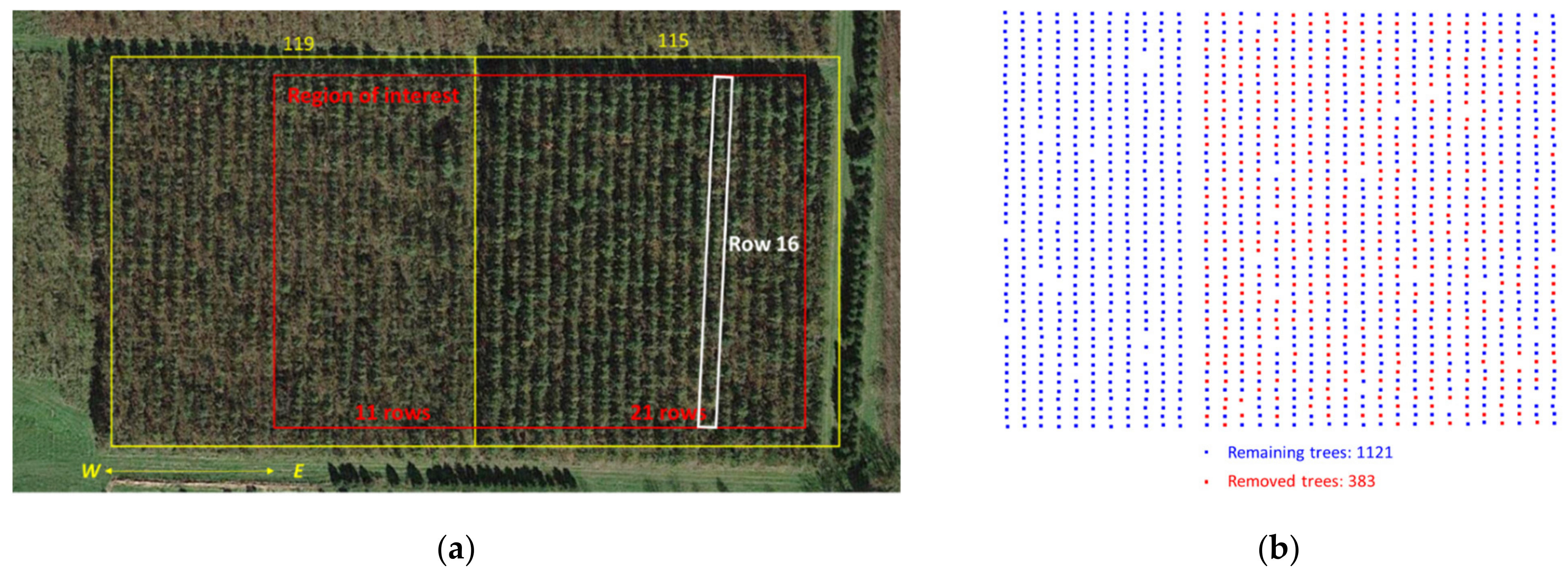
2.2. Study Site and Dataset Description

2.2.1. Study Site

The data collection site is located at Martell Forest, a research forest owned and managed by Purdue University, in West Lafayette, IN, USA. The study site consists of two plantation plots (shown in Figure 3a)—Plot 115 and Plot 119—which were planted in 2007 and 2008, respectively. The region of interest (ROI) contains 11 rows from Plot 119 and 21 rows from Plot 115. Row 16 in Plot 115 (highlighted by the white box in Figure 3a) will be used in the qualitative analysis in the experimental results (in Section 4). The main species of these two plots is northern red oak (Quercus rubra) with burr oak (Q. macrocarpa) as the training species. Trees in these two plots were planted in a grid pattern. The row spacing (east–west direction) was approximately 5 m, and adjacent tree spacing in a given row (north-south direction) was approximately 2.5 m. The tree heights ranged from 10 to 12 m when measured at year 13. The average DBH was 11.3 cm and 12.7 cm in Plots 119 and 115, respectively. The understory vegetation, e.g., herbaceous species and voluntary seedlings, was controlled on an annual basis for Plot 115 but not in Plot 119. In 2021, there were in total of 1504 trees in the ROI. It should be noted that a tree-thinning activity took place in late February 2022 on Plot 115, and 383 trees were cut down, as shown in Figure 3b.

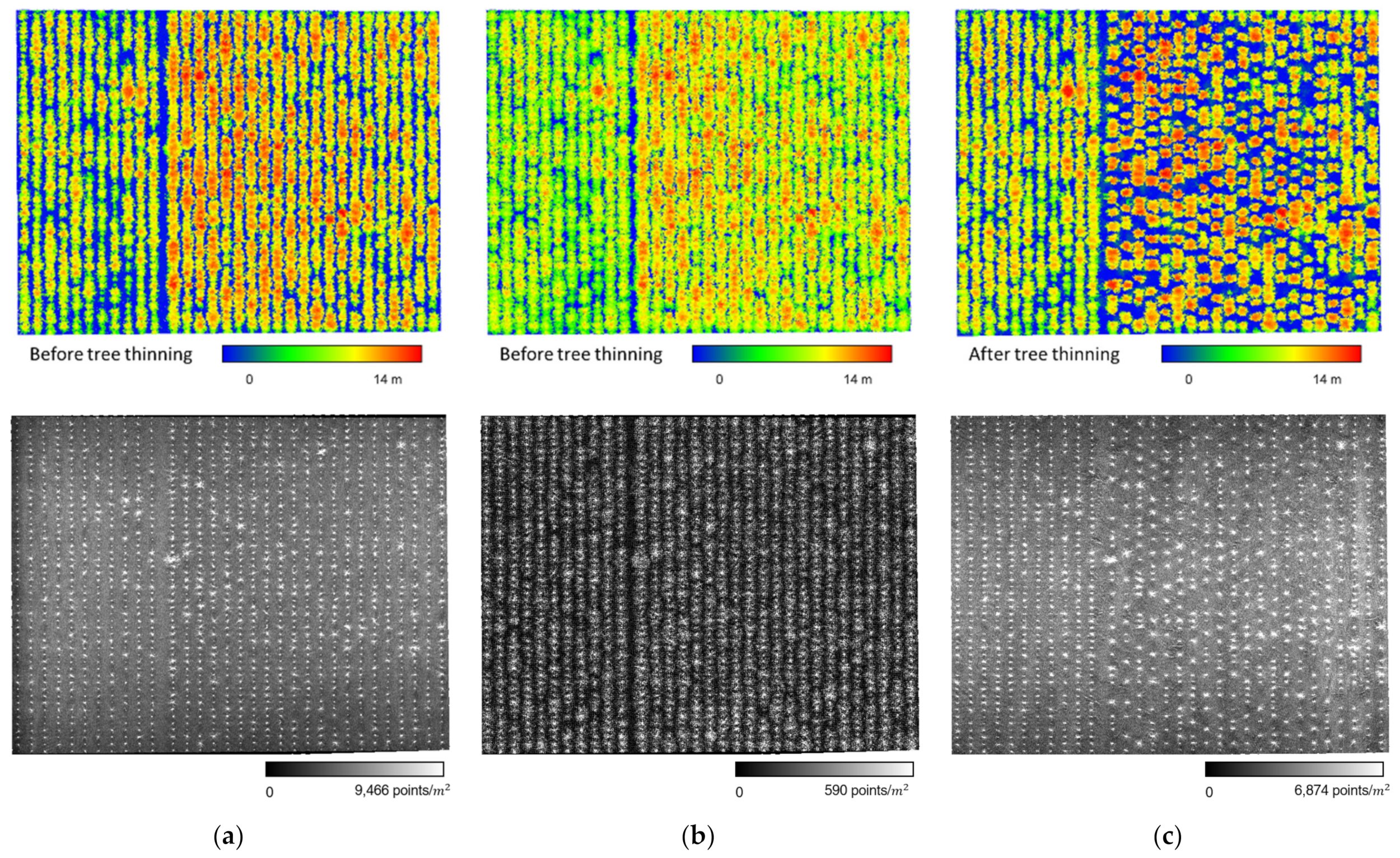
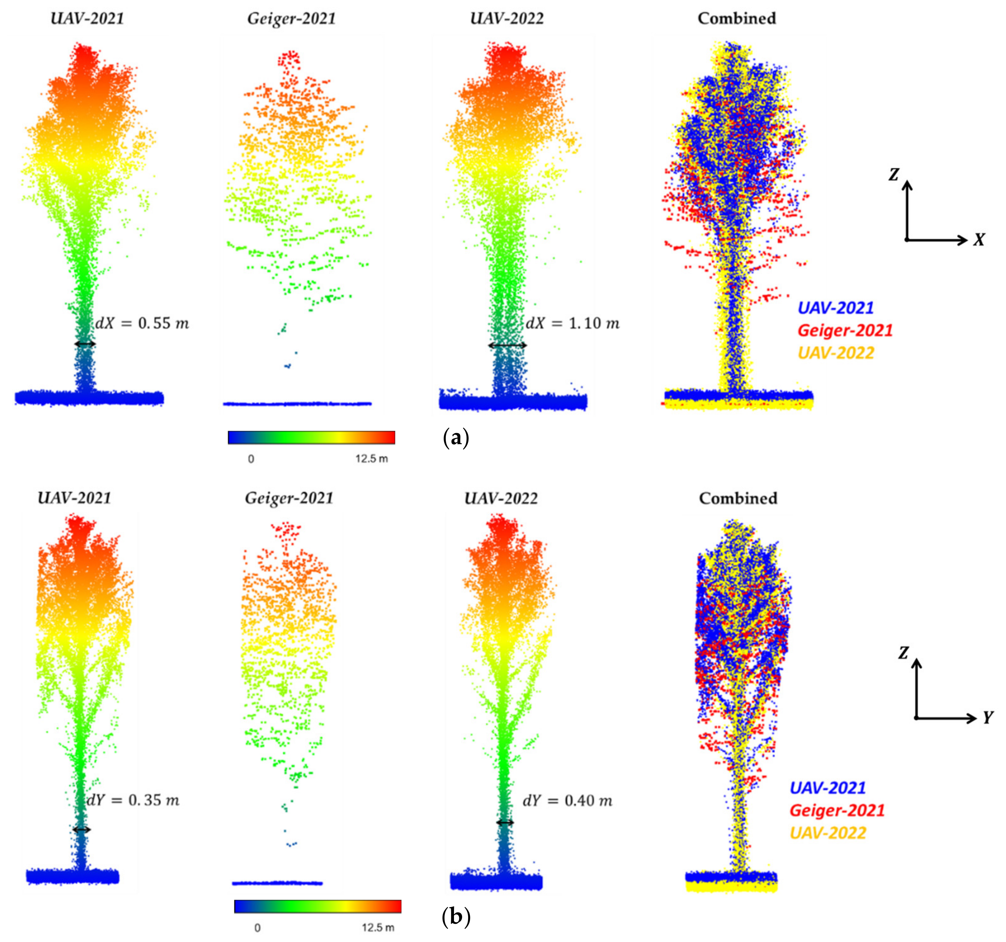
2.2.2. Dataset Description

Three datasets were collected in this study over the ROI on different dates: (i) LiDAR data collected by UAV-1 on 13 March 2021 (denoted as dataset UAV-2021), (ii) LiDAR data collected by Geiger mode system on 12 December 2021 (denoted as dataset Geiger-2021), and (iii) LiDAR data collected by UAV-2 on 3 March 2022 (denoted as dataset UAV-2022). UAV-2021 and Geiger-2021 datasets were acquired before the tree-thinning activity, while the UAV-2022 dataset was acquired afterwards. The detailed information and characteristics of these datasets are introduced below:

UAV-2021: This dataset was captured by the UAV-1 system on 13 March 2021. The UAV was flown at 40 m above-ground at a speed of 3.5 m/s. The lateral distance between adjacent flight lines was 11m. The side lap percentage of the point cloud is 95% when considering ± 70° off-nadir reconstruction. As mentioned in Section 2.1.1, the horizontal and vertical accuracy of the derived point cloud is within the range of 5–6 cm at nadir position. The dataset has high point density and geometric accuracy. The reconstructed point cloud after normalizing the height information relative to the ground level (i.e., normalized height point cloud) [41] and density map of this dataset are shown in Figure 4a. The height normalization step will be introduced in the Section 3.

Geiger-2021: This dataset was collected and processed by VeriDaaS Corporation under the USGS QL1 specifications. The vertical accuracy is better than 10 cm and the nominal spacing is less than 35 cm—i.e., nominal pulse density is more than 8 points per square meter. The data were acquired on 12 December 2021 at an altitude of approximately 3700 m above ground. Data processing began with an initial refinement to achieve a point density of 50 points per square meter over flat terrain. Then, the point cloud was spatially manipulated by aligning points in overlapping flight lines through a block adjustment procedure. This block adjustment procedure can improve the point cloud quality by compensating for inherent georeferencing errors introduced by the GNSS/INS system. The estimated accuracy of the post-processed point cloud is 5 cm along the vertical direction, which meets the USGS QL0 specifications. The normalized height point cloud and point density for this dataset are shown in Figure 4b.

UAV-2022: This dataset was captured by the UAV-2 system on 3 March 2022. The only difference in flight configuration between UAV-2022 and UAV-2021 datasets is the lateral distance between neighboring flight lines—the distance is 13 m in this dataset. This leads to a side lap percentage of about 80%. The normalized height point cloud (colored by height) and density map of the UAV-2022 dataset are shown in Figure 4c. The point density is a little lower than that of the UAV-2021 dataset. As mentioned before, data acquisition was conducted after tree-thinning activity. During this management practice, a large amount of tree debris was left at the study site. Figure 5 presents the normalized height point clouds in the 1–3 m height range for the UAV-2021 and UAV-2022 datasets. It can be seen from the figures that the UAV-2021 dataset has a very clear definition of tree locations while the debris within Plot 115 in the UAV-2022 dataset is visible, thus leading to the expected difficulties in the tree detection and localization process, as will be shown in the Section 4. Moreover, it is worth mentioning that the mounting parameters of the UAV-2 system are out-of-date. This leads to the relatively low geometric accuracy of the UAV-2022 dataset. Figure 6 shows a sample tree from the abovementioned datasets. Among them, UAV-2021 provides the best tree definition, with high point density and geometric accuracy. On the other hand, a misalignment of around 0.5 m in the X direction can be observed from the UAV-2022 dataset due to the inaccurate mounting parameters, while the alignment in the Y direction is relatively good. In terms of the Geiger-2021 dataset, the point density is low, and the definition of the tree trunk is not complete. These datasets with different characteristics were used to analyze the performance of the tree detection and localization approaches.

3. Methodology

In this section, an overview is given of the procedures for tree detection, localization, and segmentation framework (Section 3.1). Then, in Section 3.2, detailed descriptions of the DBSCAN-based, height/density-based, and proposed height-difference-based tree detection and localization approaches are presented. Lastly, the LiDAR system calibration using tree trunks and terrain patches is introduced.

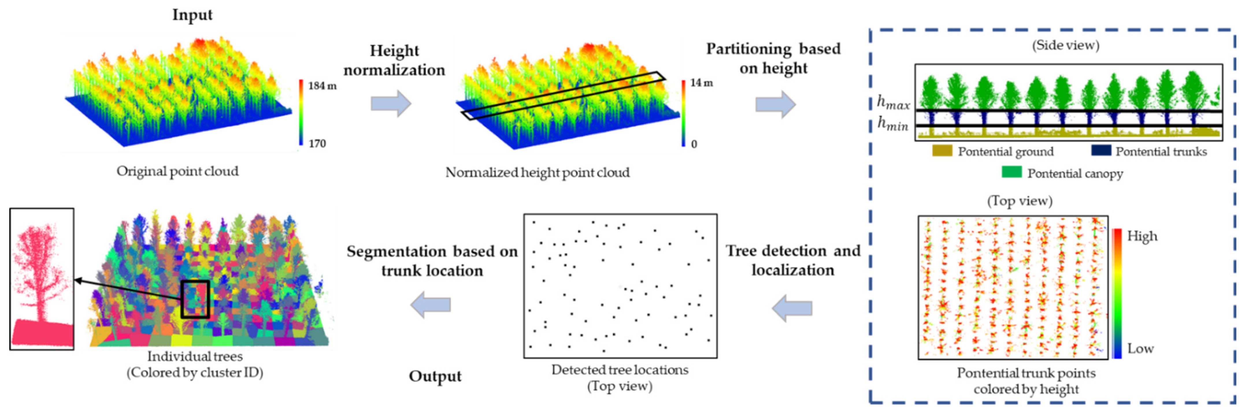
3.1. General Workflow for Tree Detection, Localization, and Segmentation

In this study, tree detection, localization, and segmentation are conducted through four main stages: point cloud height normalization, the partitioning of potential trunk points, the detection and localization of tree trunks, and individual tree segmentation. This is schematically illustrated in Figure 7. As mentioned in Section 1, three different strategies will be adopted at the third stage in this framework for comparative analysis. In this subsection, a summary of each stage will be introduced.

To begin with, a ground filtering algorithm—the adaptive cloth simulation [65]—is applied to the original LiDAR point cloud for DTM generation. This algorithm improves the original cloth simulation [66] by redefining the rigidness of each particle on the cloth according to the point density of the initially defined bare-earth point cloud. By doing so, the impact of the uneven, sparse point cloud distribution along the lower canopy on DTM generation is mitigated. Then, the point cloud normalization is carried out by subtracting the corresponding ground height from each LiDAR point. As a result, the height information of the normalized height point cloud is relative to the ground level. In the second stage, potential LiDAR points corresponding to trunks (hereafter denoted as hypothesized trunk portion) are extracted from the normalized height point cloud through user-defined minimum ($h_{min}$) and maximum ($h_{max}$) height thresholds, as illustrated in Figure 7. In this case, the majority of the canopy and shrub part is removed, leaving only the portion that is believed to correspond to trunks [51].

In the third stage, tree detection and localization are performed using the partitioned point cloud from the previous step. In this study, three different approaches were applied based on different hypotheses. In the DBSCAN-based approach, only the density information is considered, where a higher point density is assumed to be associated with tree locations. The height/density-based approach hypothesizes that a higher point density, along with higher elevation, corresponds to tree locations. Different from the two existing strategies, the proposed height-difference-based approach relies on tree geometry, assuming that high local height differences correspond to tree locations. These approaches will be presented in the next subsection. Lastly, individual trees are segmented from the normalized height point cloud based on the estimated trunk locations and 2D distance. More specifically, each LiDAR point is assigned to the tree with the closest planimetric distance. In this sense, a 2D Voronoi diagram is established along the XY plane using the trunk locations, as shown in Figure 7.

3.2. Tree Detection and Localization Strategies

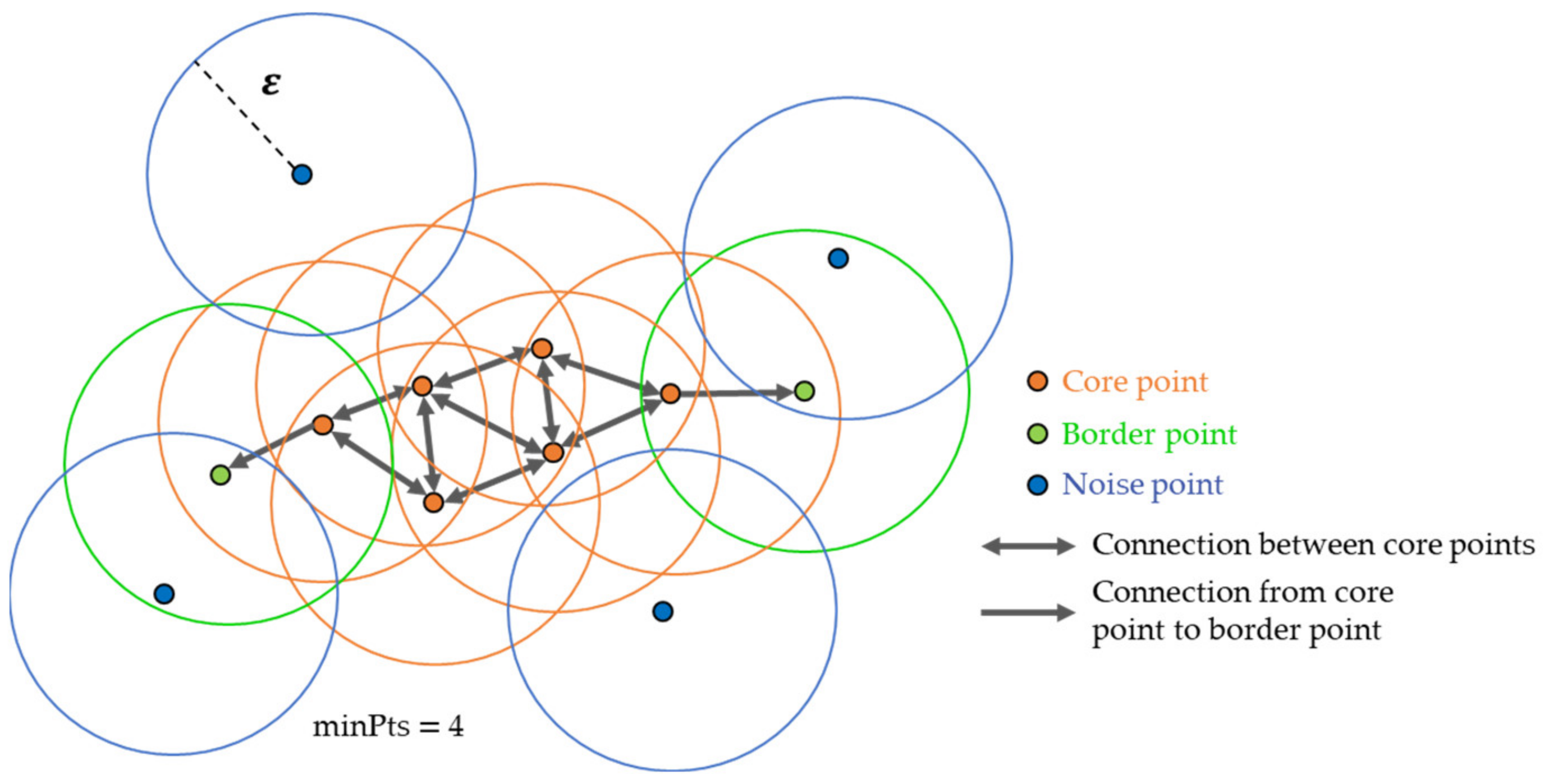
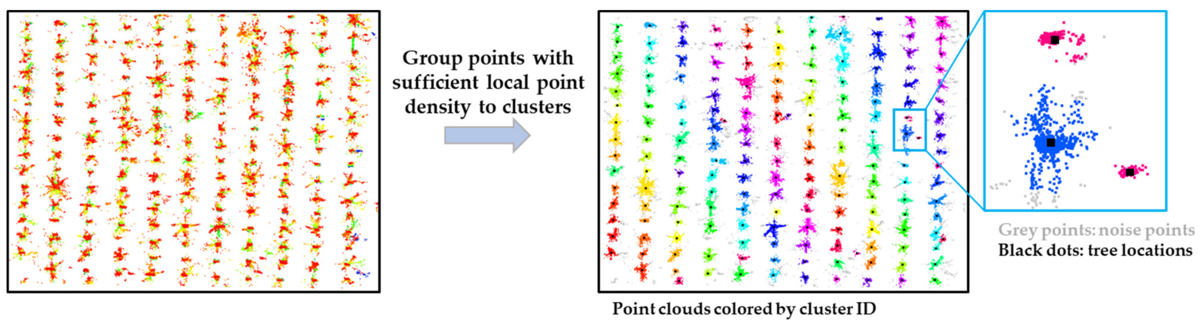
3.2.1. DBSCAN-Based Approach

The use of a DBSCAN algorithm to detect and locate trunks relies on the hypothesis that higher point density corresponds to tree location. DBSCAN is an algorithm developed to detect clusters in large spatial datasets with noise [67,68]. This algorithm requires two pre-defined thresholds: the neighborhood distance threshold denoted by $\epsilon$ and the minimum number of neighboring points $minPts$. Three types of points are defined by DBSCAN: core points, border points, and noise points. Starting from a random seed point $P_1$ that has not been classified, the number of points in this neighborhood with the radius of $\epsilon$ is counted. If the number of points (including the seed point itself) is not smaller than $minPts$, this seed point $P_1$ is defined as a core point. Then, the same procedure is performed on the neighboring points $P_2$ of this core point $P_1$. If enough neighboring points are identified, this point $P_2$ is considered a core point that is connected to core point $P_1$; otherwise, this point is considered a border point. The process subsequently identifies core points and border points from existing seed points until no new core points are identified. Ultimately, the connected core points and border points form a cluster (i.e., an individual tree in this study). The remaining points with insufficient points in their neighborhood are classified as noise points. The above steps are illustrated in Figure 8. It is worth mentioning that, in this study, the DBSCAN algorithm is performed on the planimetric coordinates of the LiDAR points. All LiDAR points within the hypothesized trunk portion are either included in clusters or classified as noise points. Finally, the trunk location is computed as the centroid of the respective cluster. Figure 9 illustrates a sample result from the DBSCAN-based approach.

A summary of involved parameters and the strategy for determining these parameters are listed below:

• Neighborhood distance threshold, $\epsilon$: The distance threshold is chosen based on prior knowledge about the diameter of the majority of trees.
• Minimum number of neighboring points, $minPts$: This parameter is dependent on the 2D point density related to trunks. Visual inspection of the partitioned point clouds and fine-tuning need to be conducted to come up with an appropriate value.

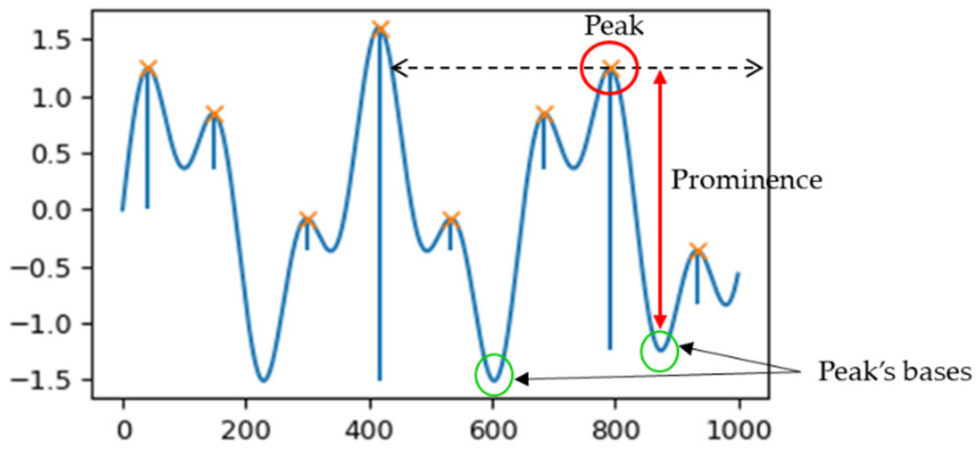
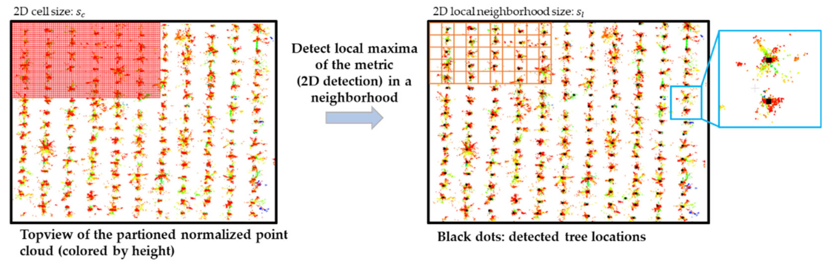
3.2.2. Height/Density-Based Approach

The height/density-based tree detection and localization approach was proposed by Lin et al. [51] based on the hypothesis that a higher point density and higher elevation correspond to trunk locations. Initially, 2D cells with size of $s_c$ are created along the XY plane over the hypothesized trunk portion. The sum of elevations of all points within each cell is evaluated. This metric reflects the point density and height of the point cloud in a local neighborhood. Then, a 2D peak detection process is carried out to identify the local maxima of the metric, which would correspond to trunk locations. Two parameters are used for peak detection: size of the square local neighborhood in 2D ($s_l$) and minimum prominence of a peak ($p_{min}$). The former is used to define the region where, at most, one peak can be selected as a detected tree, while the latter is a measurement of how much a peak stands out from the surrounding bases of the signal, as illustrated in Figure 10 for a 1-D case. For each peak, a horizontal line (dashed line in the figure) from the current peak is extended until it either reaches the border of the local neighborhood or intersects with the signal at the slope of a higher peak. Within this range, the base with the largest value is used to compute the prominence $p$ as the difference between the peak and this base. For each local neighborhood, the peak with the largest prominence value is selected as a detected tree as long as the value is larger than $p_{min}$. Moreover, the tree location is derived as the center of this cell. A sample result illustrating the height/density-based approach is shown in Figure 11.

In summary, the parameters and strategy used to determine the parameters for this approach are listed below:

• 2D cell size, $s_c$: This parameter is chosen based on the knowledge of the level of details/density that can be captured by LiDAR systems on tree trunks. If a small threshold is selected, the derived metrics will be noisy, as there are not enough points to describe a tree trunk in the neighborhood. On the other hand, choosing a large $s_c$ will affect the prediction accuracy of the tree locations.
• 2D local neighborhood size, $s_l$: Given that only one tree will be detected from a local neighborhood, the size is determined based on prior knowledge related to tree spacing within the ROI.
• Minimum prominence, $p_{min}$: This parameter needs to be fine-tuned for each dataset since it is related to the 2D point density, which depends on technical factors pertaining to data acquisition, as well as the height range for the hypothesized trunk portion.

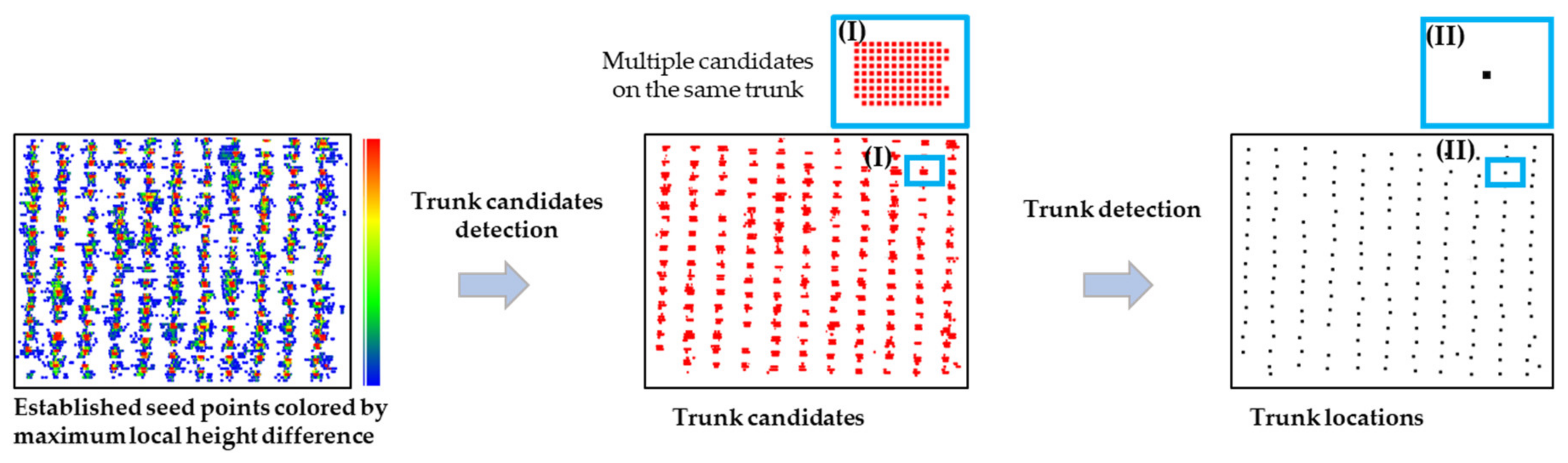
3.2.3. Height-Difference-Based Approach

To avoid the requirement for fine-tuning the parameters, we proposed a tree detection and localization approach that does not rely on point density. Instead, tree geometry is used in this approach by assuming that the tree trunk grows vertically and high local height differences correspond to trunk locations. Using the partitioned normalized height point cloud as input, tree detection and localization are performed in three main steps: estimation of maximum local height difference within a local neighborhood, trunk candidate selection, and trunk detection/localization, as illustrated in Figure 12.

The maximum local height difference estimation starts with the creation of uniformly distributed seed points with a spacing of $d_{seed}$ along the XY plane over the hypothesized trunk portion. For each seed point, a vertical cylinder centered at this point with radius $r_{cyl}$ and infinite height was created. The maximum local height difference value of this seed point was computed using the largest/smallest height from the points within this cylinder. To speed up the search process for finding LiDAR points within a cylinder, a KD-Tree was created for the partitioned point cloud. In case the maximum local height difference value of a given seed point was larger than a predefined threshold $h\_di{f}_{min}$, this point was considered a trunk candidate point. By doing this, several candidate points can be identified for a single tree trunk. In the next step, all candidate points are sorted based on the computed height different values. The candidate point with the largest value is regarded as the detected tree location. Then, neighboring candidate points with a planimetric distance from this tree location that is smaller than a user-defined threshold $d\_trun{k}_{min}$ are removed. The same steps are conducted on the remaining candidate points to derive all tree locations.

A summary of the parameters and strategy used to determine these parameters is listed below:

• Spacing between seed points, $d_{seed}$: The spacing is determined based on the prior knowledge of average tree diameter and the level of details captured by LiDAR systems on tree trunks. This parameter should be small enough to ensure that there are several seed points for a tree trunk. However, choosing a small $d_{seed}$ will result in a longer processing time.
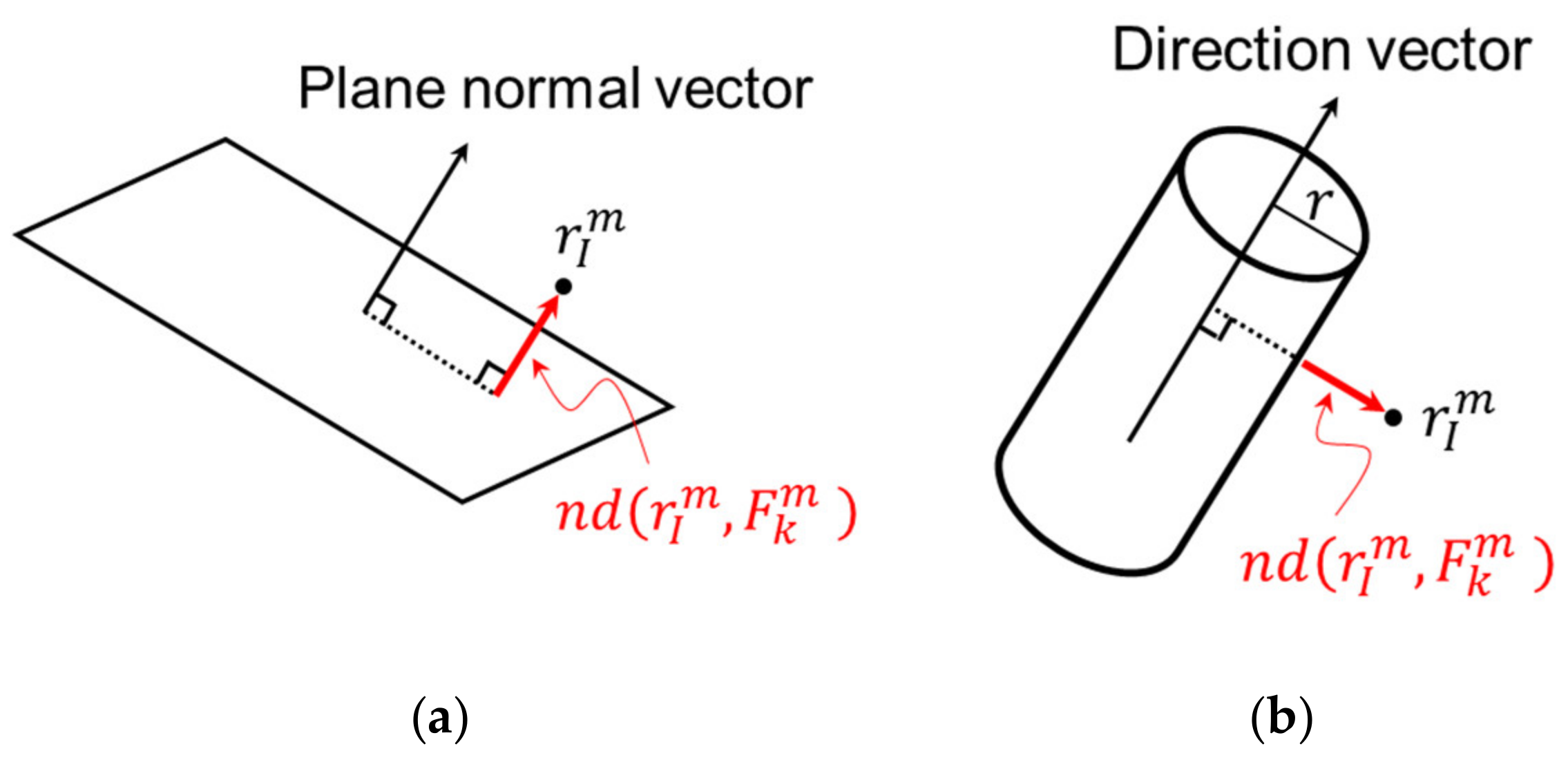
• Cylinder radius, $r_{cyl}$: This parameter also depends on the prior knowledge of average tree diameter and the level of details captured by the LiDAR system on tree trunks. More specifically, $r_{cyl}$ is chosen to guarantee that: (i) the cylinder radius is at a similar level to the trunk diameter and (ii) the cylinder contains an adequate number of LiDAR points.
• Minimum height difference value, $h\_di{f}_{min}$: This height difference threshold depends on the $h_{max}$ and $h_{min}$ values used in the partitioning step. In general, this value can be selected as from 1/2 to 2/3 of $\left(h_{max}-h_{min}\right)$.
• Minimum distance between trunks, $d\_trun{k}_{min}$: This distance is determined based on prior knowledge related to the tree spacing within the ROI.

3.3. UAV System Calibration Using Tree Trunks and Terrain Patches

As mentioned in Section 2, the mounting parameters of the UAV-2 system are out-of-date, leading to an inaccurate point cloud. Point cloud misalignment is observed at the tree trunks as well as the terrain. In this study, we proposed a novel UAV LiDAR system calibration approach relying on the identified features in a forest. The features used for the calibration process include tree trunks and planar patches. The former are modeled as cylindrical features; the latter are modeled as planar features. The conceptual basis of such calibration is that inaccurate system calibration parameters will result in a misalignment of LiDAR points corresponding to the same feature. By minimizing the discrepancy related to these features, system calibration parameters can be refined through a non-linear least-squares adjustment (LSA) process.

The feature extraction procedure is presented first. The adaptive cloth simulation algorithm [65] is adopted on the original LiDAR point cloud to generate DTM and separate bare-earth points from above-ground points. More specifically, LiDAR points whose heights are in the range of $H_{min}$ and $H_{max}$ (e.g., 1.5 m and 3.5 m) above the DTM are extracted as the above-ground point cloud portion pertaining to the trunks, while the ones whose heights are no higher than a certain value (e.g., 0.5 m) above the DTM form the bare-earth point cloud. Despite the inaccurate mounting parameters, we can observe that the level of discrepancy in the tree trunk is relatively small (within 1.0 m, as shown in Section 2.2.2). Given this, tree locations detected in the previous steps are used as seed points to identify the corresponding LiDAR points from the above-ground point cloud. More specifically, for a detected tree, its planimetric location ($X_t,Y_t$) is used to derive the ground height $Z_G$ from the DTM. Then, the seed point that corresponds to the above-ground point cloud is defined as ($X_t,Y_t,Z_G+\mathsf{\Delta }Z$), where $\mathsf{\Delta }Z$ is a user-defined height above ground (in this study, $\mathsf{\Delta }Z$ is chosen as somewhere between $H_{min}$ and $H_{max}$ values; e.g., 2.5 m). For each seed point, a spherical region with a predefined radius (e.g., 0.5 m) is created. LiDAR points from the above-ground point cloud within this spherical region are used to determine whether a cylindrical feature exists using Principal Component Analysis (PCA) [69]. If a cylindrical feature exists, the parameters of the best-fitting cylinder are estimated via an iterative model fitting and outlier removal. Region-growing is then performed to sequentially augment the neighboring points that belong to the current feature if their normal distance from the fitted cylinder is smaller than a multiplication factor times the RMSE of the fitted model. The augmenting process proceeds until no more points can be added to the feature in question. As a result, LiDAR points belonging to individual trees and the feature parameters representing the cylinder model are derived. In terms of terrain patches’ extraction, seed points that are uniformly distributed in 2D are generated over the ROI where the Z coordinates are derived from DTM. These seed points are then used to extract terrain patches from the bare-earth point cloud. Similar to tree trunk extraction, for each seed point, its neighboring LiDAR points are used to check if a plane exists, and, if yes, to derive the plane parameters through an iterative plane-fitting. Through a sequentially augmentation process, LiDAR points belonging to terrain patches and plane parameters are derived. The derived tree trunks and terrain patches are used to refine the mounting parameters through LSA.

Before discussing the details of the LSA process, a mathematical model for deriving 3D geospatial information from LiDAR is presented. LiDAR data reconstruction is based on the point positioning equation, as represented by Equation (1). In this equation, $r_I^{lu\left(t\right)}$, which is derived from raw LiDAR measurements at the firing time (including range measurement and orientation of the laser beam relative to the laser unit reference frame), denotes the position of the laser beam footprint relative to the laser unit frame; $r_{b\left(t\right)}^m$ and $R_{b\left(t\right)}^m$ are the position and orientation information of the IMU body frame coordinate system relative to the mapping frame at firing time $t$; $r_{lu}^b$ and $R_{lu}^b$ represent the lever arm and boresight rotation matrix relating the laser unit system and IMU body frame; and $r_I^m$ is the coordinates of object point $I$ in the mapping frame.

$$r_I^m=r_{b\left(t\right)}^m+R_{b\left(t\right)}^m{r}_{lu}^b+R_{b\left(t\right)}^m{R}_{lu}^b{r}_I^{lu\left(t\right)}$$

(1)

The mathematical model of the LSA involves observation equations—i.e., the normal distance—coming from cylindrical and planar features, as graphically illustrated and mathematically introduced in Figure 13 and Equation (2), respectively. The LSA estimates mounting parameters to minimize the weighted squared sum of the normal distances between each LiDAR point and its corresponding parametric model, as presented in Equation (3). Here, $F_k^m$ represents the feature parameters for the $k^{th}$ feature in the mapping frame; $nd\left(r_I^m,F_k^m\right)$ denotes the normal distance between the LiDAR point $I$ and its corresponding feature $F_k^m$; $w_{F_k^m}$ is the weight of the normal distance observation relative to each feature, which is assigned based on the expected accuracy. Considering that the UAV system was operated in open sky with continuous accessibility to GNSS signal, the derived post-processed trajectory is relatively accurate. Therefore, trajectory information—i.e., $r_{b\left(t\right)}^m/R_{b\left(t\right)}^m$—is fixed in the LSA, while mounting parameters and feature parameters are refined.

$$nd\left(r_I^m,F_k^m\right)=0$$

(2)

$$\underset{r_{lu}^b,R_{lu}^b,F_k^m}{\mathrm{argmin}} {\displaystyle \sum _{\forall \mathrm{points} \mathrm{and} \mathrm{features}}}{w}_{F_k^m}{\left(nd\left(r_I^m,F_k^m\right)\right)}^2$$

(3)

4. Experimental Results

This section starts by introducing system calibration results for the UAV-2022 dataset. Next, a comparative evaluation of the three tree detection and localization strategies used to deal with point clouds with different characteristics will be presented.

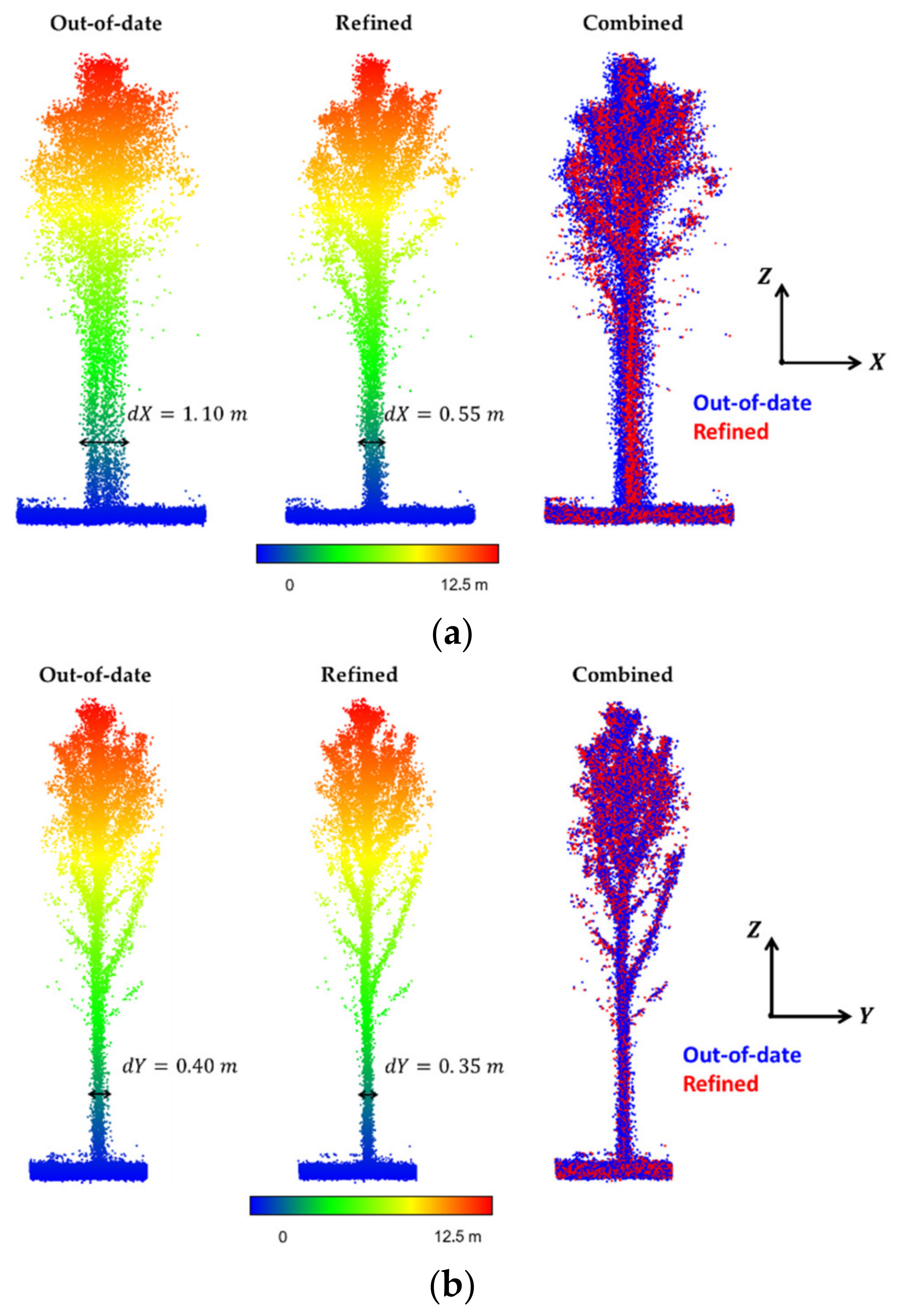
4.1. System Calibration Results for UAV-2022 Dataset

The proposed system calibration approach using tree trunks and terrain patches was conducted on the UAV-2022 dataset. Figure 14 shows the extracted features for calibration. In total, 406 tree trunks and 3095 terrain patches were derived. The expected accuracy for normal distance related to these features was set to 5 cm. In the LSA process, LiDAR boresight angles ($\mathsf{\Delta }\omega$, $\mathsf{\Delta }\varphi$, $\mathsf{\Delta }\kappa$), as well as lever arm components in X and Y directions ($\mathsf{\Delta }X$ and $\mathsf{\Delta }Y$), were estimated. The Z lever arm component was fixed, as it requires vertical control [70]. The derived square root of a posteriori variance factor (${\widehat{\sigma }}_0$) of the LSA is 1.15, which is close to 1. This reveals that the assigned a priori variances for the LiDAR observations are reasonable. The initial (i.e., out-of-date) and refined system calibration parameters, along with their STD values, are presented in

Table 1. Initial (out-of-date) and refined system calibration parameters using the proposed system calibration approach for the UAV-2022 dataset.

Mounting Parameters	$\mathbf{\Delta }\mathit{\omega }\left(°\right)$	$\mathbf{\Delta }\mathit{\varphi }\left(°\right)$	$\mathbf{\Delta }\mathit{\kappa }\left(°\right)$	$\mathbf{\Delta }\mathit{X}\left(\mathit{m}\right)$	$\mathbf{\Delta }\mathit{Y}\left(\mathit{m}\right)$	$\mathbf{\Delta }\mathit{Z}\left(\mathit{m}\right)$
Initial	1.261	−0.276	0.129	−0.115	0.022	0.100
Refined	1.217 ±0.001	−0.307 ±0.001	−0.121 ±0.002	−0.101 ±0.001	0.024 ±0.001	N\A

. The STD values for the estimated mounting parameters are small. Moreover, it has been observed that the estimated mounting parameters are not highly correlated. Based on the low correlation and small STDs of the estimated parameters, one can conclude that the LiDAR mounting parameters are accurately estimated using the proposed strategy. Additionally, by comparing the refined mounting parameters to the out-of-date ones in Table 1, most of the mounting parameters remain stable, except for the $\mathsf{\Delta }\kappa$ angle, which exhibits a change of 0.25 degrees.

The system calibration results are evaluated both qualitatively and quantitatively. Figure 15 presents a sample tree from the UAV-2 system using the inaccurate and refined mounting parameters. It can be seen from this figure that the misalignment was minimized (mainly in the X direction) after the system calibration and the resulting point cloud have similar level of geometric accuracy to the UAV-2021 dataset (Figure 6). To quantify the performance of the proposed system calibration approach,

Table 2. Quantitative evaluation of point cloud alignment before and after system calibration.

	Number of Features	Number of Points	Before Calibration			After Calibration
			Mean (m)	STD (m)	RMSE (m)	Mean (m)	STD (m)	RMSE (m)
Tree Trunks	406	~196,000	0.094	0.128	0.159	0.061	0.063	0.088
Terrain Patches	3095	~19,847,000	0.076	0.089	0.117	0.039	0.042	0.057

reports the mean, STD, and RMSE values of normal distances from the LiDAR feature points to their corresponding best-fitting cylinder/plane before and after mounting parameter refinement. The achieved improvements in the RMSE values range from 16 cm to 9 cm and 12 cm to 6 cm for tree trunks and terrain patches, respectively.

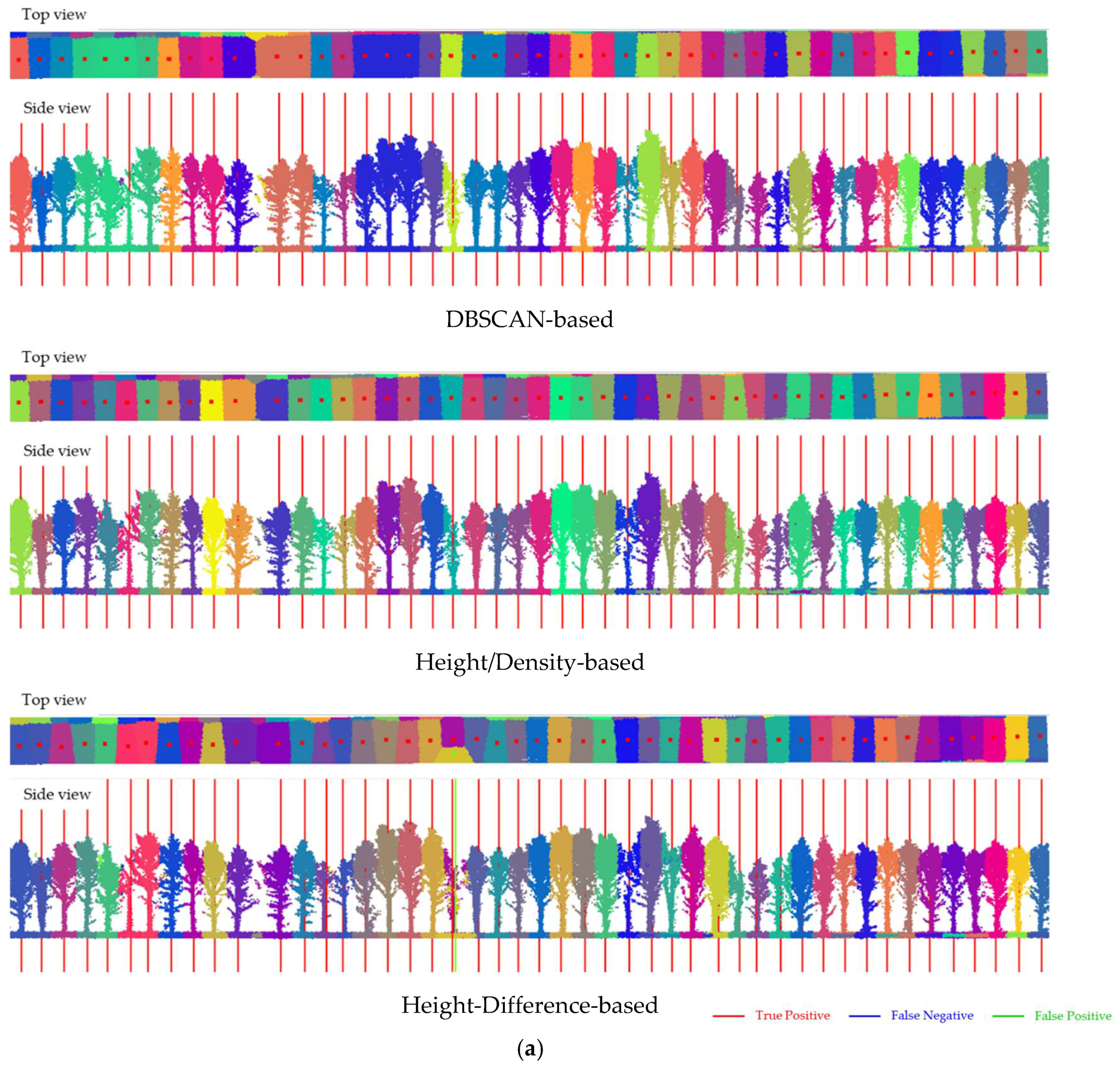
4.2. Comparative Evaluation of Different Tree Detection and Localization Approaches

In this study, three datasets collected by two UAV LiDAR systems (datasets UAV-2021 and UAV-2022) and one Geiger Mode LiDAR system (dataset Geiger-2021) were used to evaluate the tree detection, localization, and segmentation results. As introduced in Section 4.1, LiDAR mounting parameters from the UAV-2 system were refined. The LiDAR point clouds from the UAV-2022 dataset were reconstructed using both the out-of-date and refined mounting parameters (hereafter denoted as UAV-2022-Low-Acc and UAV-2022-High-Acc). The common framework with the three different tree detection and localization approaches was applied to the four LiDAR point clouds. The utilized parameters/thresholds for each approach, as well as the height range thresholds $h_{min}$ and $h_{max}$ for partitioning the tree trunk areas relative to each dataset, are listed in

Table 3. Utilized parameters/thresholds for the DBSCAN-based, height/density-based, and height-difference-based approaches for the four LiDAR point clouds.

Parameters/Thresholds		UAV-2021	Geiger-2021	UAV-2022-Low/High-Acc
DBSCAN-Based	$h_{min} \left(m\right)$	1.0	1.0	2.0
	$h_{max} \left(m\right)$	3.0	3.0	3.5
	$\epsilon \left(m\right)$	0.5	0.5	0.5
	$minPts$	100	7	80
Height/Density-based	$h_{min} \left(m\right)$	1.0	1.0	2.0
	$h_{max} \left(m\right)$	3.0	3.0	3.5
	$s_c \left(m\right)$	0.1	0.1	0.1
	$s_l \left(m\right)$	2.0	2.0	2.0
	$p_{min} \left(m\right)$	11.5	2.0	10.0
Height-Difference-based	$h_{min} \left(m\right)$	1.5	1.5	2.5
	$h_{max} \left(m\right)$	5.0	5.0	5.0
	$d_{seed} \left(m\right)$	0.1	0.1	0.1
	$r_{cyl} \left(m\right)$	0.2	0.2	0.2
	$h\_di{f}_{min} \left(m\right)$	2.0	2.0	1.5
	$d\_trun{k}_{min} \left(m\right)$	1.0	1.0	1.0

. For UAV-2021 and Geiger-2021 datasets, the height range was set to 1.0–3.0 m for DBSCAN-based and height/density-based approaches and 1.5–5.0 m for the height-difference-based approach. As the height-difference-based approach determines tree location purely based on the height information, a larger height range was selected to improve robustness. Due to the existing debris in the UAV-2022 dataset, the range thresholds were set to be higher compared to those for the 2021 datasets to remove LiDAR points corresponding to such debris. As described in the Section 3, the $minPts$ and $p_{min}$ for the DBSCAN-based and height/density-based approaches are highly dependent on the point density; thus, they were fine-tuned to reach the optimal results for each dataset. On the other hand, parameters for the height-difference-based approach were determined intuitively.

The performance of the tree detection and localization approaches was evaluated using manually identified reference data. These data were acquired by examining the LiDAR point clouds to identify individual trees and estimate the tree locations. Point cloud from the UAV-2021 was used to derive these data, and 1504 trees were identified. A total of 383 trees were cut down in this area in late February 2022. Therefore, the reference data are only valid for the UAV-2021 and Geiger-2021 datasets. Then, the UAV-2022-High-Acc point cloud was used to identify removed trees to derive the reference data (1121 trees) for the UAV-2022 dataset. The manually measured tree locations were expected to have centimeter-level accuracy. The detected tree locations from the different approaches were compared to those from the reference data. According to prior knowledge related to the geometric accuracy of the utilized point clouds, the accuracy of correctly detected tree locations is expected to be better than 1 m. Given this, if the planimetric distance between two locations is smaller than 1 m, we consider them to be a valid pair. The performance of tree detection using different datasets/approaches was evaluated through the number of true positives (TP), false positives (FP), and false negatives (FN), as well as the corresponding precision, recall, and F1 score (as presented in Equations (4)–(6)). In terms of the tree location accuracy, the mean, standard deviation (STD), and root–mean–square error (RMSE) values of the X and Y coordinate differences between the true positives from the proposed strategies and manually established reference data are also reported.

$$\mathrm{Precision}=\frac{\mathrm{TP}}{\mathrm{TP}+\mathrm{FP}}$$

(4)

$$\mathrm{Recall}=\frac{\mathrm{TP}}{\mathrm{TP}+\mathrm{FN}}$$

(5)

$$\mathrm{F}1 \mathrm{score}=2\times \frac{\mathrm{Precision}\times \mathrm{Recall}}{\mathrm{Precision}+\mathrm{Recall}}$$

(6)

The impact of different characteristics of the LiDAR point clouds on the performance of the tree detection and localization approaches were evaluated as follows: (i) impact of point density was analyzed by comparing results from UAV-2021 and Geiger-2021; (ii) impact of geometric accuracy was analyzed by comparing results from UAV-2022-Low-Acc and UAV-2022-High-Acc; and (iii) impact of environmental complexity (in this study, the debris from the cut trees) was analyzed by comparing results from UAV-2021 and UAV-2022-High-Acc. The remaining subsections start by presenting the tree detection and localization results of these dataset/point cloud pairs. Next, the processing time for the three approaches to each dataset/point cloud is listed to evaluate their computational efficiency.

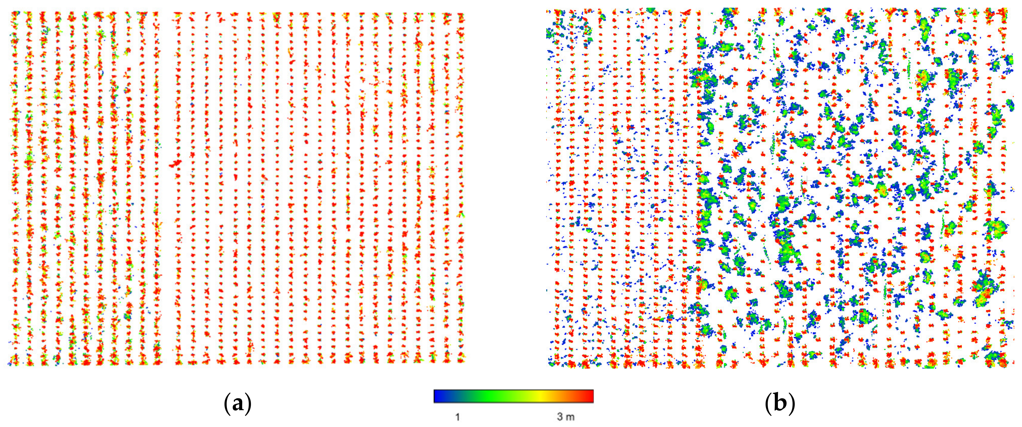
4.2.1. Impact of Point Density on Tree Detection and Localization

To evaluate the impact of point density, UAV-2021 and Geiger-2021 datasets were used for comparison.

Table 4. Performance of the tree detection and localization approaches on UAV-2021 and Geiger-2021 datasets.

UAV-2021
	NRD	NDT	TP	FN	FP	Precision	Recall	F1 score
DBSCAN	1504	1502	1499	5	3	0.998	0.997	0.997
Height/Density		1505	1502	2	3	0.998	0.999	0.998
Height-Difference		1514	1501	3	13	0.991	0.998	0.995
Geiger-2021
	NRD	NDT	TP	FN	FP	Precision	Recall	F1 score
DBSCAN	1504	1255	1114	390	141	0.888	0.741	0.808
Height/Density		1816	1238	266	578	0.682	0.823	0.746
Height-Difference		1617	1408	96	209	0.871	0.936	0.902

lists the number of trees in the reference data $N_{RD}$, number of detected trees $N_{DT}$, number of TP, FN, and FP, as well as the precision, recall, and F1 score metrics for these datasets when using the different approaches. For the UAV-2021 dataset with high point density, all three approaches successfully detected the majority of trees, as indicated by the low FN and high recall values. However, the two density-based approaches outperformed the height-difference-based approach that falsely detected 13 trees. Considering that the height-difference-based approach does not heavily rely on point density information, like the other approaches, it is more sensitive to noise and/or points from other objects, such as debris, understory vegetation, and low branches. In the case of low point density, the performance of all approaches dramatically deteriorates. The height-difference-based approach resulted in the greatest number of true positives and the highest F1 score. This is expected, as the other two approaches are more sensitive to density information.

Based on the detected true positives, an accuracy assessment of the tree localization results was conducted using the reference data.

Table 5. Tree localization accuracy assessment on UAV-2021 and Geiger-2021 datasets.

	UAV-2021						Geiger-2021
	$\mathrm{Mean} \left(m\right)$		$\mathrm{STD} \left(m\right)$		$\mathrm{RMSE} \left(m\right)$		$\mathrm{Mean} \left(m\right)$		$\mathrm{STD} \left(m\right)$		$\mathrm{RMSE} \left(m\right)$
	$dX$	$dY$	$dX$	$dY$	$dX$	$dY$	$dX$	$dY$	$dX$	$dY$	$dX$	$dY$
DBSCAN	0.007	−0.004	0.086	0.075	0.086	0.075	−0.220	0.035	0.261	0.274	0.341	0.276
Height/Density	0.011	0.002	0.090	0.077	0.091	0.077	−0.175	0.035	0.291	0.253	0.339	0.256
Height-Difference	0.004	0.000	0.177	0.212	0.177	0.212	−0.226	0.063	0.249	0.254	0.336	0.262

reports the mean, STD, and RMSE values of the X, Y coordinate differences. The results for UAV-2021 suggest that the tree locations derived from the DBSCAN-based and height/density-based approaches achieve an accuracy of 0.1 m when the LiDAR point cloud is accurate and dense. However, due to the nature of deriving trunk location from the height-difference-based approach, errors were introduced. As a result, STD values from the height-difference-based approach are larger (around 0.2 m). By looking at the results from the Geiger-2021 dataset, a constant shift can be observed, of around −0.2 m in the X direction and 0.05 m in the Y direction. This can be attributed to the misalignment between the datasets from UAV and Geiger mode LiDAR, as the reference data were established using the former. Due to the low point density and incomplete definition for the trunks in the Geiger-2021 dataset, all approaches exhibited larger STD values in the tree localization results. Overall, similar tree localization results were achieved in the Geiger-2021 dataset for all approaches.

To provide a closer view of the tree detection, localization, and segmentation results using the three approaches, Figure 16 shows the top and side views of the segmented normalized point clouds and detected tree locations for row 16 in plot 115 for the UAV-2021 and Geiger-2021 datasets. In this figure, the correct detections (true positives) are shown in red, false negatives are shown in blue, and false positives are shown in green. The results suggest that these approaches’ performance in the UAV-2021 dataset is good and the detections align well with the tree trunks. By looking into results from the Geiger-2021 dataset, false negatives and false positives tend to occur with small and undeveloped trees that are close to the neighboring trees, or in areas where very few points are related to the trunks. Among all strategies, height-difference-based approaches resulted in the lowest number of false negatives (i.e., two in this row).

4.2.2. Impact of Geometric Accuracy on Tree Detection and Localization

In this subsection, LiDAR point clouds are reconstructed from the same dataset using the inaccurate and accurate LiDAR mounting parameters to evaluate the impact of geometric accuracy. The tree detection results of the three approaches are presented in

Table 6. Performance of the tree detection and localization approaches on UAV-2022-Low-Acc and UAV-2022-High-Acc point clouds.

UAV-2022-Low-Acc
	NRD	NDT	TP	FN	FP	Precision	Recall	F1 score
DBSCAN	1121	1121	1111	10	10	0.991	0.991	0.991
Height/Density		1109	1104	17	5	0.996	0.985	0.990
Height-Difference		1143	1116	5	27	0.976	0.996	0.986
UAV-2022-High-Acc
	NRD	NDT	TP	FN	FP	Precision	Recall	F1 score
DBSCAN	1121	1123	1113	8	10	0.991	0.993	0.992
Height/Density		1123	1116	5	7	0.994	0.996	0.995
Height-Difference		1140	1117	4	23	0.980	0.996	0.988

. For the height/density-based approach, tree detection results from the point cloud with worse geometric accuracy introduced more false negatives (the number increases from 5 to 17). For the point cloud, LiDAR points corresponding to an individual tree tend to be dispersed due to the misalignment, thus leading to peaks with lower prominence values compared to the point cloud with high accuracy. The DBSCAN-based approach is less sensitive to inaccurate point clouds (the number of false negatives from inaccurate point clouds is only two more than that those from the accurate point cloud). A possible reason for this different sensitivity to inaccurate point clouds could be the neighborhood distance threshold ($\epsilon =0.5 m$) used for the DBSCAN-based approach and cell size ($s_c=0.1 m$) for the height/density-based approach. More specifically, for a point cloud with a misalignment of around 0.5 m, its effect on the point density within a local neighborhood with a radius of 0.5 m is relatively smaller than that on the metrics derived from a cell with 0.1 m. In addition, in terms of the remaining metrics listed in Table 6, similar results can be observed from the UAV-2022-Low-Acc and UAV-2022-High-Acc point clouds for each strategy. This suggests that the level of misalignment from the UAV-2022-Low-Acc point cloud does not significantly affect the tree detection results. Moreover, by comparing the results from the three approaches, one could note that the height-difference-based approach successfully detected the largest number of correct trees (true positive), resulting in the most commission errors (false positive) in the meantime. This finding is compatible with the observation in Section 4.2.1.

Table 7. Tree localization accuracy assessment on UAV-2022-Low-Acc and UAV-2022-High-Acc point clouds.

	UAV-2022-Low-Acc						UAV-2022-High-Acc
	$\mathrm{Mean} \left(m\right)$		$\mathrm{STD} \left(m\right)$		$\mathrm{RMSE} \left(m\right)$		$\mathrm{Mean} \left(m\right)$		$\mathrm{STD} \left(m\right)$		$\mathrm{RMSE} \left(m\right)$
	$dX$	$dY$	$dX$	$dY$	$dX$	$dY$	$dX$	$dY$	$dX$	$dY$	$dX$	$dY$
DBSCAN	0.004	−0.001	0.186	0.084	0.186	0.084	0.008	−0.006	0.098	0.089	0.098	0.089
Height/Density	0.034	−0.010	0.190	0.093	0.193	0.094	0.031	−0.010	0.094	0.087	0.099	0.088
Height-Difference	0.002	−0.006	0.292	0.212	0.292	0.212	0.005	−0.002	0.175	0.197	0.175	0.197

lists the accuracy of the estimated tree locations based on the two point clouds. It can be observed from this table that STD values for X differences from the UAV-2022-Low-Acc point cloud are larger than those from the UAV-2022-High-Acc point cloud, while the values for Y differences are close. This is because the misalignment in the UAV-2022-Low-Acc mainly occurs along the X direction, as shown in Figure 6 and Figure 15. Given that the results from these two point clouds are relatively similar, the qualitative result for the UAV-2022 dataset will be presented in the next subsection, and compared to the UAV-2021 dataset.

4.2.3. Impact of Environmental Complexity on Tree Detection and Localization

Although UAV-2021 and UAV-2022-High-Acc point clouds have a similar point density and geometric accuracy, large amounts of tree debris were present in the latter as the tree-thinning activity created a complex and challenging environment for tree detection and localization. These two point clouds are used to analyze the effect of environmental complexity on tree detection and localization results.

Table 8. Performance of the tree detection and localization approaches on UAV-2021 and UAV-2022-High-Acc point clouds.

UAV-2021
	NRD	NDT	TP	FN	FP	Precision	Recall	F1 score
DBSCAN	1504	1502	1499	5	3	0.998	0.997	0.997
Height/Density		1505	1502	2	3	0.998	0.999	0.998
Height-Difference		1514	1501	3	13	0.991	0.998	0.995
UAV-2022-High-Acc
	NRD	NDT	TP	FN	FP	Precision	Recall	F1 score
DBSCAN	1121	1123	1113	8	10	0.991	0.993	0.992
Height/Density		1123	1116	5	7	0.994	0.996	0.995
Height-Difference		1140	1117	4	23	0.980	0.996	0.988

presents the tree detection results of the three approaches. Although height range thresholds ($h_{min}$ and $h_{max}$) for the UAV-2022-High-Acc were adjusted to avoid including the majority of LiDAR points from the debris in the tree detection process, the numbers of false negatives and false positives in all approaches are still higher than those from the UAV-2021 point cloud. Among these values, the number of false positives for the height-difference-based approach increases the most. Although similar numbers of true positives were achieved by all approaches, the height-difference-based approach resulted in the most false positives for both point clouds. This indicates that the height-difference-based approach is prone to being affected by points from other objects (debris) in the dataset. The positional/localization accuracy of correctly detected tree locations is shown in

Table 9. Tree localization accuracy assessment on UAV-2021 and UAV-2022-High-Acc point clouds.

	UAV-2021						UAV-2022-High-Acc
	$\mathrm{Mean} \left(m\right)$		$\mathrm{STD} \left(m\right)$		$\mathrm{RMSE} \left(m\right)$		$\mathrm{Mean} \left(m\right)$		$\mathrm{STD} \left(m\right)$		$\mathrm{RMSE} \left(m\right)$
	$dX$	$dY$	$dX$	$dY$	$dX$	$dY$	$dX$	$dY$	$dX$	$dY$	$dX$	$dY$
DBSCAN	0.007	−0.004	0.086	0.075	0.086	0.075	0.008	−0.006	0.098	0.089	0.098	0.089
Height/Density	0.011	0.002	0.090	0.077	0.091	0.077	0.031	−0.010	0.094	0.087	0.099	0.088
Height-Difference	0.004	0.000	0.177	0.212	0.177	0.212	0.005	−0.002	0.175	0.197	0.175	0.197

. By comparing the mean, STD, and RMSE values from the two point clouds using the same approach, the differences are within 3 cm, which is smaller than the expected accuracy of the point clouds. Therefore, we can conclude that the debris does not affect the tree localization results.

Figure 17 shows top and side views of the segmented normalized height point clouds and detected tree locations for row 16 in plot 115 for the UAV-2021 and UAV-2022-High-Acc datasets. By comparing the normalized height point clouds from the two datasets, the trees removed from the thinning activity can easily be observed. Without the debris, the terrain in the UAV-2021 dataset is cleaner compared to that in the UAV-2022 dataset. Although the tree density in the UAV-2021 dataset is higher than the UAV-2022 dataset, the three detection and localization approaches show promising performance. When dealing with the UAV-2022-High-Acc point cloud after the thinning activity, the debris on the site leads to more false positives in the height-difference-based results (i.e., three in this row).

4.2.4. Processing Time for Tree Detection and Localization Approaches

In this subsection, the processing time for each approach is compared. All experiments were conducted on a computer with Intel^® Core™ i7-6700 Processor and 16GB memory.

Table 10. Processing time for the tree detection and localization approaches on the three datasets.

Dataset	Approach	Number of Points (Million)	Processing Time (s)
UAV-2021	DBSCAN	1.7	439.0
	Height/Density	1.7	21.6
	Height-Difference	3.7	69.1
UAV-2022-High-Acc	DBSCAN	1.1	41.1
	Height/Density	1.1	15.0
	Height-Difference	2.0	51.9
Geiger-2021	DBSCAN	0.3	3.9
	Height/Density	0.3	5.8
	Height-Difference	0.8	39.1

lists the processing times for the three tree detection and localization approaches. As the UAV-2022-Low/High-Acc point clouds have the same number of points and a close processing time, only the results for UAV-2021, UAV-2022-High-Acc, and Geiger-2021 are presented. For the UAV datasets with a high point density, the height/density-based approach had the best performance in terms of processing time. For the dataset with low density (e.g., Geiger-2021 dataset), both DBSCAN-based and height/density-based approaches have a similar performance. Moreover, it can be observed from the table that the processing time for the DBSCAN-based approach dramatically increases as the number of points increases, while the other two slightly increase.

5. Discussion

This study investigated the performance of three different tree detection and localization strategies—DBSCAN-based, height/density-based, and the proposed height-difference-based approaches—when dealing with point clouds with different characteristics. The first two approaches rely on point density information to detect tree locations using point clouds representing the trunk areas. Therefore, the thresholds for these two approaches (i.e., $minPts$ and $p_{min}$, respectively) need to be fine-tuned to derive the optimal results. On the other hand, the proposed height-difference-based approach detects individual trees based on the maximum height differences between points in a local neighborhood. Although more thresholds are required for this approach, their values are selected intuitively based on general prior knowledge related to the datasets and ROI (e.g., species/age of trees and nominal average tree spacing) without the requirements for trial-and-error/fine-tuning. Nevertheless, using only height information will lead to misdetection when LiDAR points from other objects exist in the point cloud—i.e., low branches (~4–5 m height), and debris (~1–3 m height) within the same planimetric locations will easily lead to a falsely detected tree. The performance of these three approaches in terms of tree detection can be summarized as follows:

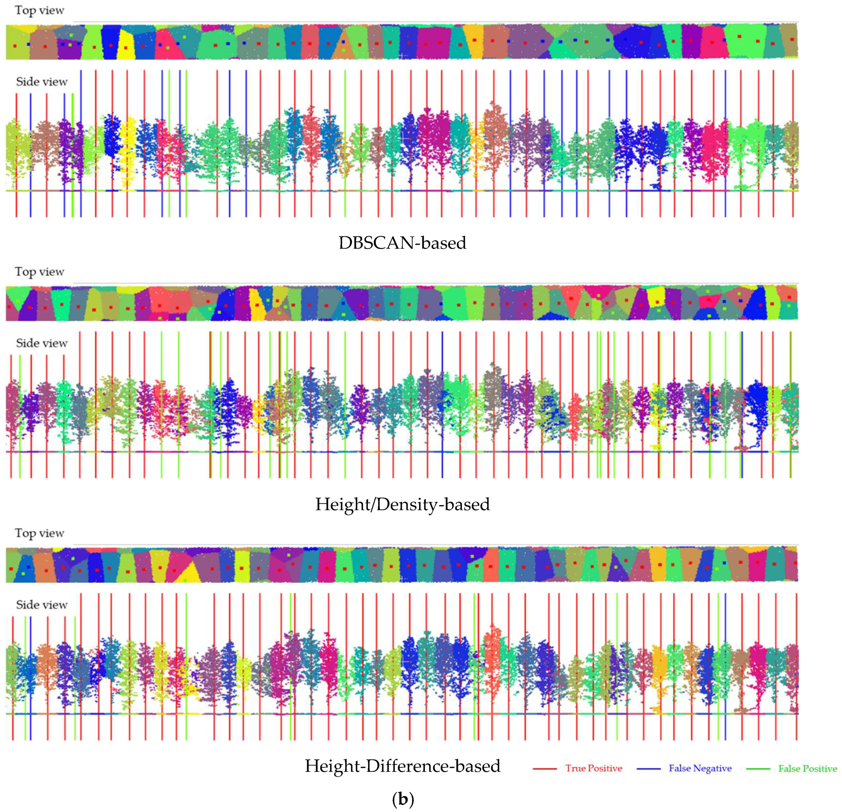
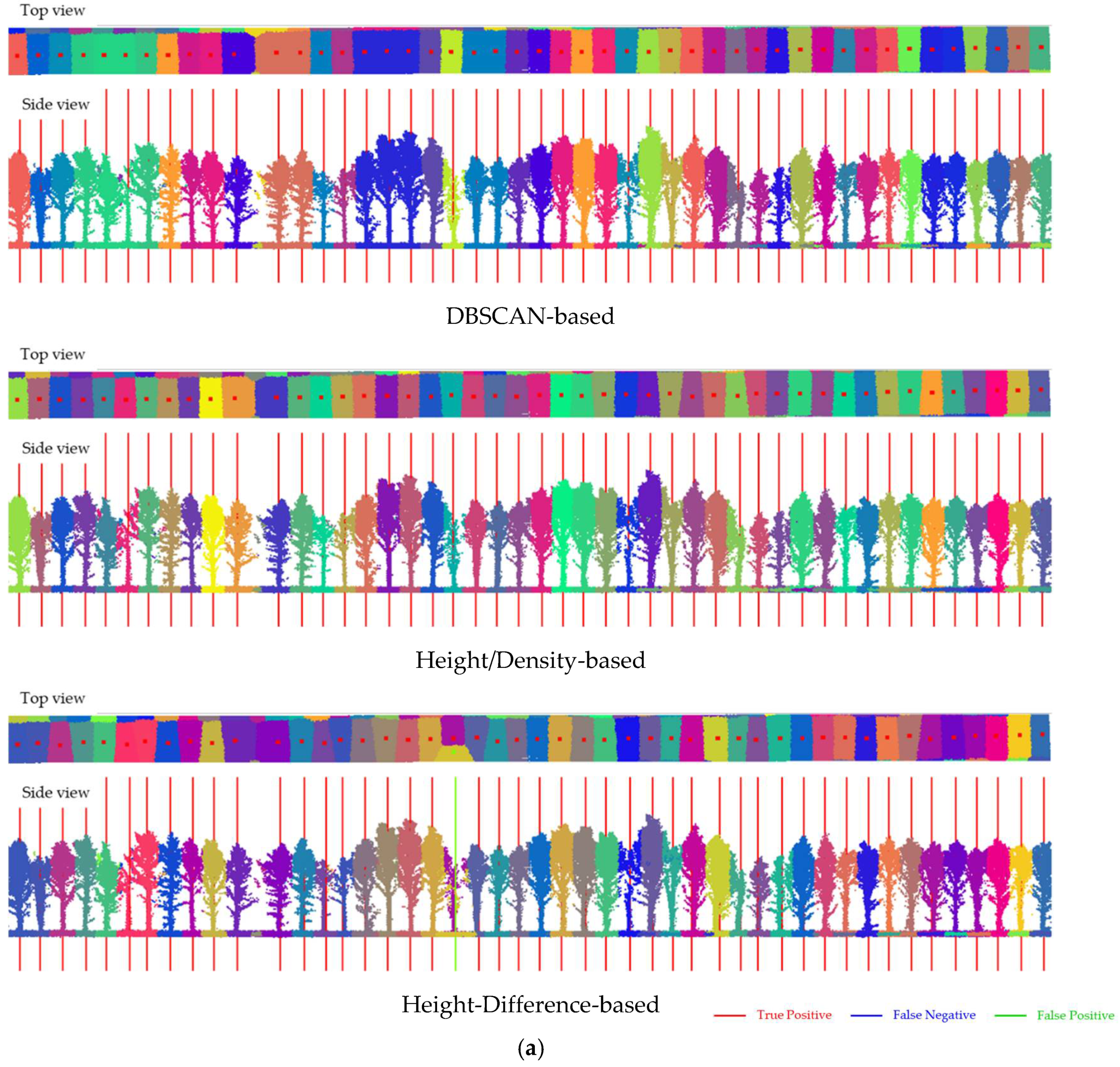
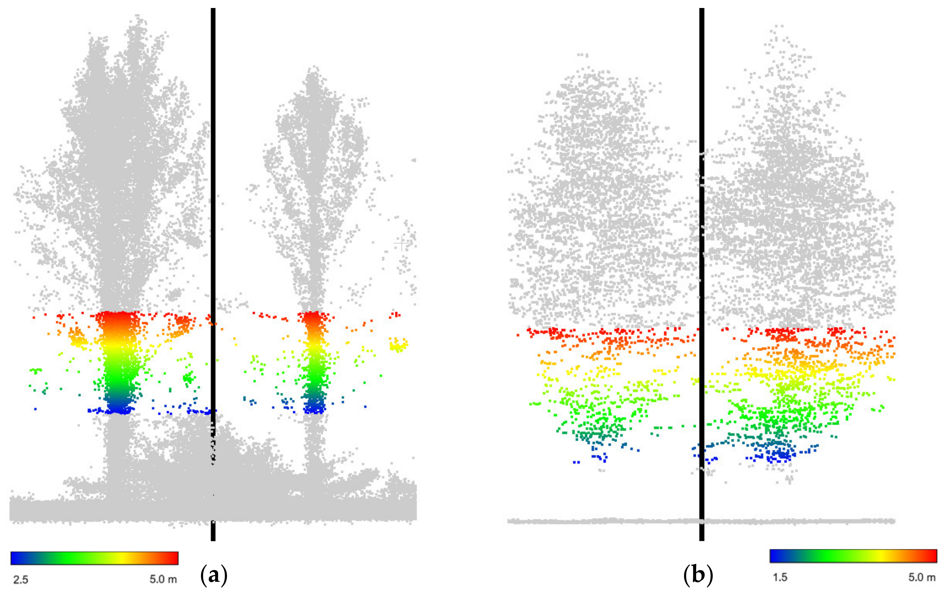
• After fine-tuning the parameters related to DBSCAN-based and height/density-based approaches, comparative tree detection results were achieved from the UAV point clouds with adequate point density—the F1 scores for UAV-2021 and UAV-2022-Low/High-Acc point clouds are higher than 0.99 regardless of the geometric accuracy and environmental complexity. The height-difference-based approach produced similar results to other two approaches when applied on high-density UAV point clouds with slightly more false positives. This is expected since the height-difference-based approach is prone to noise and/or points from other objects such as debris, understory vegetations, and low branches. One sample of detected false positives from UAV-2022-High-Acc is shown in Figure 18a, where points from the debris and low branches resulted in a falsely detected tree.
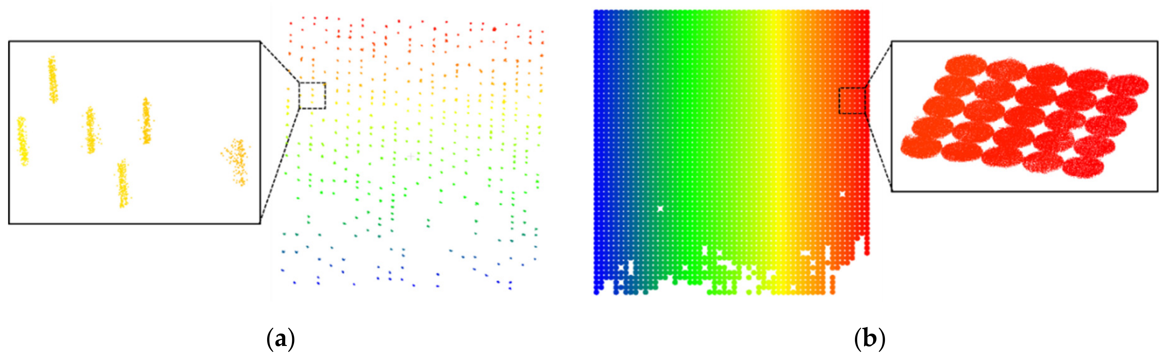
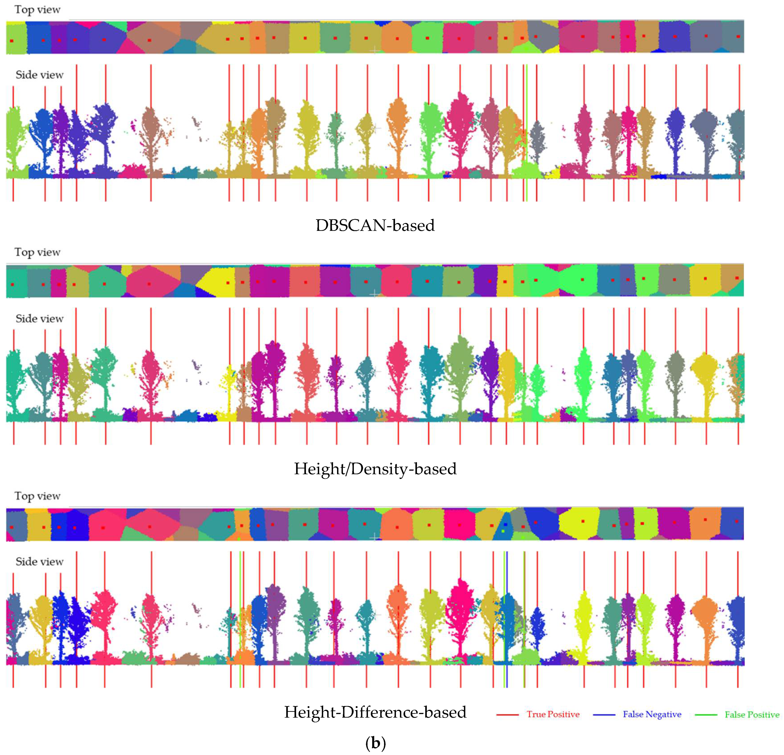
• In terms of the Geiger-2021 dataset with low point density, the performance of all approaches dramatically deteriorated. Among them, the height-difference-based approach correctly detected the greatest number of trees, followed by the height/density-based and DBSCAN-based approaches. This is expected as the height-difference-based approach does not rely on density information for tree detection. Figure 18b shows a commission error from the Geiger-2021 dataset. It can be observed that points from the branches and noise points between two trees lead to a false positive. By looking into false positive detections as shown in Figure 18, an additional post-processing step (i.e., a quality control process) can be proposed to remove them based on density information and/or by analyzing the vertical spatial distribution of the points within the local neighborhood. Therefore, false positive detections are preferable to false negatives, as the former can be removed relatively easily while finding omission errors is challenging. Overall, although the commission errors are higher than the DBSCAN-based approach, the height-difference-based approach is more suitable for performing tree detection for point clouds with a low point density.

In terms of tree localization, the three approaches derive the locations differently. The DBSCAN-based approach extracts a cluster that represents an individual tree and computes the centroid of the cluster as the tree location. This approach is believed to provide accurate tree locations, except for the case when points related to the tree are not uniformly distributed. On the other hand, the height/density-based approach detects the peak in the 2D cells using the sum of elevation metrics as a single tree. The center of the detected cell is then regarded as the tree location. Therefore, the accuracy of the tree location depends on the cell size ($s_c$). As the cell size was set to 0.1 cm in this study, the tree localization results from the height/density-based approach are expected to be accurate. In terms of the height-difference-based approach, the established seed point with the largest maximum height difference in the neighborhood is directly used as the tree location. The detected location does not correspond to the centroid, but to a random location on the surface of the tree trunk. As a result, the accuracy of the location is affected by (i) the size used to define the cylindrical local neighborhood ($r_{cyl}=0.2 m$) and (ii) the diameter of the tree trunk. The above analysis is verified through the localization results for the point cloud with high point density and geometric accuracy—i.e., the accuracy for the DBSCAN-based and height/density-based methods is around 0.1 m and that of the height-difference-based method is around 0.2 m. When dealing with point clouds with low density, the performance of these different approaches is comparable for tree locations. In this case, the accuracy is mainly controlled by captured details in the point cloud. Moreover, from the comparison between UAV-2022-Low-Acc and UAV-2022-High-Acc point clouds, geometric accuracy will affect the STD values of the tree locations that were derived for all approaches to a similar extent.

In terms of processing time, the height/density-based approach shows the best performance, as the steps are simple and relatively efficient. The DBSCAN-based approach has a computational complexity of $\mathrm{O}\left({\mathrm{n}}^3\right)$. As the number of points increases, the processing time of the DBSCAN-based approach dramatically increases. Therefore, this approach is not suitable for point clouds with a high level of fine detail and a high number of points. The proposed height-difference-based approach includes the step of finding points within a given local neighborhood. Although a KD-tree data structure is used to improve the efficiency, this step is still time-consuming. As a result, the height-difference-based approach requires a longer processing time than the height/density-based approach. The above findings are summarized in

Table 11. A summary of the processing time and impact of different dataset characteristics for each tree detection and localization approach.

Strategies	Processing Time	Point Density		Geometric Accuracy		Debris
		Det.	Loc.	Det.	Loc.	Det.	Loc.
DBSCAN	Medium–Slow	✓✓	✓✓	✓	✓✓	✓	✗
Height/Density	Fast	✓✓	✓✓	✗	✓✓	✓	✗
Height-Difference	Medium–Slow	✓✓	✓	✗	✓✓	✓	✗

Det.: Detection, Loc.: Localization, ✓✓: High impact, ✓: Low impact, ✗: No impact.

, where the processing time and impact of different dataset characteristics are listed for each tree detection and localization approach.

6. Conclusions

In this paper, a new trunk-based tree detection and localization approach based on the maximum height difference among point clouds in a local neighborhood was proposed. This approach was compared to two state-of-the-art trunk-based approaches—DBSCAN-based and height/density-based approaches. To evaluate their performance on point clouds with different characteristics, two UAV LiDAR datasets and one Geiger-mode LiDAR dataset over a plantation under leaf-off conditions were used. For UAV-2022 dataset, the LiDAR system calibration parameters were out-of-date, resulting in point clouds with low geometric accuracy. To resolve this issue, a novel system calibration process using tree trunks and ground patches was proposed. After refining the LiDAR mounting parameters, the point cloud from the UAV-2022 dataset achieved the same level of geometric accuracy as the one from the UAV-2021 dataset. Overall, four LiDAR point clouds with different point densities, geometric accuracies, and environmental complexities were used to conduct a comparative analysis of these approaches according to the tree detection and localization accuracy, as well as the execution time. Experimental results from the UAV datasets suggested that DBSCAN-based and height/density-based approaches perform well in terms of tree detection (F1 score > 0.99) and localization (with an accuracy of 0.1 m for point clouds with high geometric accuracy) after fine-tuning the thresholds. However, the processing time of the latter is much quicker than that of the former. In general, the height-difference-based approach can extract the majority of trees from UAV datasets without fine-tuning the thresholds. However, due to the limitation of the algorithm, the tree location accuracy is worse than that of the other two approaches. On the other hand, results from the Geiger mode dataset with low point density showed that the performance of all approaches dramatically deteriorated. Among them, the proposed height-difference-based approach resulted in the greatest number of true positives and highest F1 score, making it most suitable for point clouds with low density without the need for fine-tuning parameters.

The main limitation of the proposed height-difference-based approach is the direct use of a seed point with a large maximum height difference as the tree location. This significantly affects the accuracy of the derived locations. To overcome this issue, future work will focus on proposing a more robust localization algorithm based on detected trees. Future work will also focus on augmenting the tree detection results by incorporating a quality control procedure. More specifically, by analyzing the distribution of point clouds close to the detected trees, false positives can be removed. Furthermore, the performance of these trunk-based approaches on natural forests will be investigated. Lastly, the derivation of other forest inventory metrics—e.g., stem map and wood volume—will be explored.

References

1. Fahey, T.J.; Woodbury, P.B.; Battles, J.J.; Goodale, C.L.; Hamburg, S.P.; Ollinger, S.V.; Woodall, C.W. Forest Carbon Storage: Ecology, Management, and Policy. Front. Ecol. Environ. 2010, 8, 245–252. [Google Scholar] [CrossRef] [Green Version]
2. Bettinger, P.; Boston, K.; Siry, J.P.; Grebner, D.L. Forest Management and Planning, 2nd ed.; Academic Press: Cambridge, MA, USA, 2017. [Google Scholar]
3. Kangas, A.S. Value of Forest Information. Eur. J. For. Res. 2010, 129, 1263–1276. [Google Scholar] [CrossRef]
4. West, P.W. Tree and Forest Measurement; Springer: Berlin/Heidelberg, Germany, 2009. [Google Scholar]
5. Hoppus, M.L.; Lister, A.J. Measuring Forest Area Loss over Time Using FIA Plots and Satellite Imagerye. Proc. Fourth Annu. For. Inventory Anal. Symp. 2005, 252, 91–97. [Google Scholar]
6. Ohmann, J.L.; Gregory, M.J. Predictive Mapping of Forest Composition and Structure with Direct Gradient Analysis and Nearest-Neighbor Imputation in Coastal Oregon, U.S.A. Can. J. For. Res. 2002, 32, 725–741. [Google Scholar] [CrossRef]
7. Foody, G.M.; Boyd, D.S.; Cutler, M.E.J. Predictive Relations of Tropical Forest Biomass from Landsat TM Data and Their Transferability between Regions. Remote Sens. Environ. 2003, 85, 463–474. [Google Scholar] [CrossRef]
8. Hudak, A.T.; Robichaud, P.R.; Evans, J.B.; Clark, J.; Lannom, K.; Morgan, P.; Stone, C. Field Validation of Burned Area Reflectance Classification (BARC) Products for Post Fire Assessment. Tenth For. Serv. Remote Sens. Appl. Conf. 2004. [Google Scholar]
9. Stepper, C.; Straub, C.; Pretzsch, H. Assessing Height Changes in a Highly Structured Forest Using Regularly Acquired Aerial Image Data. Forestry 2014, 88, 304–316. [Google Scholar] [CrossRef] [Green Version]
10. Tian, J.; Wang, L.; Li, X.; Gong, H.; Shi, C.; Zhong, R.; Liu, X. Comparison of UAV and WorldView-2 Imagery for Mapping Leaf Area Index of Mangrove Forest. Int. J. Appl. Earth Obs. Geoinf. 2017, 61, 22–31. [Google Scholar] [CrossRef]
11. Melin, M.; Korhonen, L.; Kukkonen, M.; Packalen, P. Assessing the Performance of Aerial Image Point Cloud and Spectral Metrics in Predicting Boreal Forest Canopy Cover. ISPRS J. Photogramm. Remote Sens. 2017, 129, 77–85. [Google Scholar] [CrossRef]
12. Pearse, G.D.; Dash, J.P.; Persson, H.J.; Watt, M.S. Comparison of High-Density LiDAR and Satellite Photogrammetry for Forest Inventory. ISPRS J. Photogramm. Remote Sens. 2018, 142, 257–267. [Google Scholar] [CrossRef]
13. Maltamo, M.; Næsset, E.; Vauhkonen, J. Forestry Applications of Airborne Laser Scanning: Concepts and Case Studies; Springer: Berlin/Heidelberg, Germany, 2014; Volume 27. [Google Scholar]
14. Farid, A.; Goodrich, D.C.; Bryant, R.; Sorooshian, S. Using Airborne Lidar to Predict Leaf Area Index in Cottonwood Trees and Refine Riparian Water-Use Estimates. J. Arid. Environ. 2008, 72, 1–15. [Google Scholar] [CrossRef] [Green Version]
15. Tian, L.; Qu, Y.; Qi, J. Estimation of Forest Lai Using Discrete Airborne Lidar: A Review. Remote Sens. 2021, 13, 2408. [Google Scholar] [CrossRef]
16. Meng, X.; Currit, N.; Zhao, K. Ground Filtering Algorithms for Airborne LiDAR Data: A Review of Critical Issues. Remote Sens. 2010, 2, 833–860. [Google Scholar] [CrossRef] [Green Version]
17. Chen, Z.; Gao, B.; Devereux, B. State-of-the-Art: DTM Generation Using Airborne LIDAR Data. Sensors 2017, 17, 150. [Google Scholar] [CrossRef] [PubMed] [Green Version]
18. Michałowska, M.; Rapiński, J. A Review of Tree Species Classification Based on Airborne Lidar Data and Applied Classifiers. Remote Sens. 2021, 13, 353. [Google Scholar] [CrossRef]
19. Maltamo, M.; Eerikäinen, K.; Pitkänen, J.; Hyyppä, J.; Vehmas, M. Estimation of Timber Volume and Stem Density Based on Scanning Laser Altimetry and Expected Tree Size Distribution Functions. Remote Sens. Environ. 2004, 90, 319–330. [Google Scholar] [CrossRef]
20. Packalen, P.; Vauhkonen, J.; Kallio, E.; Peuhkurinen, J.; Pitkänen, J.; Pippuri, I.; Strunk, J.; Maltamo, M. Predicting the Spatial Pattern of Trees by Airborne Laser Scanning. Int. J. Remote Sens. 2013, 34, 5154–5165. [Google Scholar] [CrossRef]
21. Hyde, P.; Dubayah, R.; Peterson, B.; Blair, J.B.; Hofton, M.; Hunsaker, C.; Knox, R.; Walker, W. Mapping Forest Structure for Wildlife Habitat Analysis Using Waveform Lidar: Validation of Montane Ecosystems. Remote Sens. Environ. 2005, 96, 427–437. [Google Scholar] [CrossRef]
22. Swatantran, A.; Dubayah, R.; Roberts, D.; Hofton, M.; Blair, J.B. Mapping Biomass and Stress in the Sierra Nevada Using Lidar and Hyperspectral Data Fusion. Remote Sens. Environ. 2011, 115, 2917–2930. [Google Scholar] [CrossRef] [Green Version]
23. Lindberg, E.; Holmgren, J. Individual Tree Crown Methods for 3D Data from Remote Sensing. Curr. For. Rep. 2017, 3, 19–31. [Google Scholar] [CrossRef] [Green Version]
24. Yu, X.; Kukko, A.; Kaartinen, H.; Wang, Y.; Liang, X.; Matikainen, L.; Hyyppä, J. Comparing Features of Single and Multi-Photon Lidar in Boreal Forests. ISPRS J. Photogramm. Remote Sens. 2020, 168, 268–276. [Google Scholar] [CrossRef]
25. Brede, B.; Lau, A.; Bartholomeus, H.M.; Kooistra, L. Comparing RIEGL RiCOPTER UAV LiDAR Derived Canopy Height and DBH with Terrestrial LiDAR. Sensors 2017, 17, 2371. [Google Scholar] [CrossRef] [PubMed]
26. Liu, K.; Shen, X.; Cao, L.; Wang, G.; Cao, F. Estimating Forest Structural Attributes Using UAV-LiDAR Data in Ginkgo Plantations. ISPRS J. Photogramm. Remote Sens. 2018, 146, 465–482. [Google Scholar] [CrossRef]
27. Corte, A.P.D.; Souza, D.V.; Rex, F.E.; Sanquetta, C.R.; Mohan, M.; Silva, C.A.; Zambrano, A.M.A.; Prata, G.; Alves de Almeida, D.R.; Trautenmüller, J.W.; et al. Forest Inventory with High-Density UAV-Lidar: Machine Learning Approaches for Predicting Individual Tree Attributes. Comput. Electron. Agric. 2020, 179, 2787. [Google Scholar] [CrossRef]
28. Chen, Q.; Gao, T.; Zhu, J.; Wu, F.; Li, X.; Lu, D.; Yu, F. Individual Tree Segmentation and Tree Height Estimation Using Leaf-Off and Leaf-On UAV-LiDAR Data in Dense Deciduous Forests. Remote Sens. 2022, 14, 2787. [Google Scholar] [CrossRef]
29. Liang, X.; Kankare, V.; Hyyppä, J.; Wang, Y.; Kukko, A.; Haggrén, H.; Yu, X.; Kaartinen, H.; Jaakkola, A.; Guan, F.; et al. Terrestrial laser scanning in forest inventories. ISPRS J. Photogramm. Remote Sens. 2016, 115, 63–77. [Google Scholar] [CrossRef]
30. Burt, A.; Disney, M.I.; Raumonen, P.; Armston, J.; Calders, K.; Lewis, P. Rapid characterisation of forest structure from TLS and 3D modelling. In Proceedings of the International Geoscience and Remote Sensing Symposium (IGARSS), Houston, TX, USA, 26–29 May 2013. [Google Scholar]
31. Heinzel, J.; Huber, M.O. Detecting Tree Stems from Volumetric TLS Data in Forest Environments with Rich Understory. Remote Sens. 2017, 9, 9. [Google Scholar] [CrossRef] [Green Version]
32. Comesaña-Cebral, L.; Martínez-Sánchez, J.; Lorenzo, H.; Arias, P. Individual Tree Segmentation Method Based on Mobile Backpack LiDAR Point Clouds. Sensors 2021, 21, 6007. [Google Scholar] [CrossRef]
33. Ko, C.; Lee, S.; Yim, J.; Kim, D.; Kang, J. Comparison of Forest Inventory Methods at Plot-Level between a Backpack Personal Laser Scanning (BPLS) and Conventional Equipment in Jeju Island, South Korea. Forests 2021, 12, 308. [Google Scholar] [CrossRef]
34. Potapov, P.; Li, X.; Hernandez-Serna, A.; Tyukavina, A.; Hansen, M.C.; Kommareddy, A.; Pickens, A.; Turubanova, S.; Tang, H.; Silva, C.E.; et al. Mapping global forest canopy height through integration of GEDI and Landsat data. Remote Sens. Environ. 2020, 253, 112165. [Google Scholar] [CrossRef]
35. Zhao, D.; Pang, Y.; Li, Z.; Liu, L. Isolating individual trees in a closed coniferous forest using small footprint lidar data. Int. J. Remote Sens. 2014, 35, 7199–7218. [Google Scholar] [CrossRef]
36. Hilker, T.; Coops, N.C.; Newnham, G.J.; van Leeuwen, M.; Wulder, M.A.; Stewart, J.; Culvenor, D.S. Comparison of Terrestrial and Airborne LiDAR in Describing Stand Structure of a Thinned Lodgepole Pine Forest. J. For. 2012, 110, 97–104. [Google Scholar] [CrossRef]
37. LaRue, E.; Wagner, F.; Fei, S.; Atkins, J.; Fahey, R.; Gough, C.; Hardiman, B. Compatibility of Aerial and Terrestrial LiDAR for Quantifying Forest Structural Diversity. Remote Sens. 2020, 12, 1407. [Google Scholar] [CrossRef]
38. Babbel, B.J.; Olsen, M.J.; Che, E.; Leshchinsky, B.A.; Simpson, C.; Dafni, J. Evaluation of Uncrewed Aircraft Systems’ Lidar Data Quality. ISPRS Int. J. Geo-Inform. 2019, 8, 532. [Google Scholar] [CrossRef] [Green Version]
39. Morsdorf, F.; Eck, C.; Zgraggen, C.; Imbach, B.; Schneider, F.D.; Kükenbrink, D. UAV-based LiDAR acquisition for the derivation of high-resolution forest and ground information. Geophysics 2017, 36, 566–570. [Google Scholar] [CrossRef]
40. Hyyppä, E.; Yu, X.; Kaartinen, H.; Hakala, T.; Kukko, A.; Vastaranta, M.; Hyyppä, J. Comparison of Backpack, Handheld, Under-Canopy UAV, and Above-Canopy UAV Laser Scanning for Field Reference Data Collection in Boreal Forests. Remote Sens. 2020, 12, 3327. [Google Scholar] [CrossRef]
41. Lin, Y.-C.; Shao, J.; Shin, S.-Y.; Saka, Z.; Joseph, M.; Manish, R.; Fei, S.; Habib, A. Comparative Analysis of Multi-Platform, Multi-Resolution, Multi-Temporal LiDAR Data for Forest Inventory. Remote Sens. 2022, 14, 649. [Google Scholar] [CrossRef]
42. Crespo-Peremarch, P.; Fournier, R.A.; Nguyen, V.-T.; van Lier, O.R.; Ruiz, L.Á. A comparative assessment of the vertical distribution of forest components using full-waveform airborne, discrete airborne and discrete terrestrial laser scanning data. For. Ecol. Manag. 2020, 473, 118268. [Google Scholar] [CrossRef]
43. Hyyppa, J.; Kelle, O.; Lehikoinen, M.; Inkinen, M. A segmentation-based method to retrieve stem volume estimates from 3-D tree height models produced by laser scanners. IEEE Trans. Geosci. Remote Sens. 2001, 39, 969–975. [Google Scholar] [CrossRef]
44. Popescu, S.; Wynne, R.H.; Nelson, R.F. Measuring individual tree crown diameter with lidar and assessing its influence on estimating forest volume and biomass. Can. J. Remote Sens. 2003, 29, 564–577. [Google Scholar] [CrossRef]
45. Koch, B.; Heyder, U.; Weinacker, H. Detection of Individual Tree Crowns in Airborne Lidar Data. Photogramm. Eng. Remote Sens. 2006, 72, 357–363. [Google Scholar] [CrossRef] [Green Version]
46. Chen, Q.; Baldocchi, D.; Gong, P.; Kelly, M. Isolating Individual Trees in a Savanna Woodland Using Small Footprint Lidar Data. Photogramm. Eng. Remote Sens. 2006, 72, 923–932. [Google Scholar] [CrossRef] [Green Version]
47. Jeronimo, S.M.A.; Kane, V.R.; Churchill, D.J.; McGaughey, R.J.; Franklin, J.F. Applying LiDAR Individual Tree Detection to Management of Structurally Diverse Forest Landscapes. J. For. 2018, 116, 336–346. [Google Scholar] [CrossRef] [Green Version]
48. Yun, T.; Jiang, K.; Li, G.; Eichhorn, M.P.; Fan, J.; Liu, F.; Chen, B.; An, F.; Cao, L. Individual tree crown segmentation from airborne LiDAR data using a novel Gaussian filter and energy function minimization-based approach. Remote Sens. Environ. 2021, 256, 112307. [Google Scholar] [CrossRef]
49. Shao, G.; Shao, G.; Fei, S. Delineation of individual deciduous trees in plantations with low-density LiDAR data. Int. J. Remote Sens. 2018, 40, 346–363. [Google Scholar] [CrossRef]
50. Li, W.; Guo, Q.; Jakubowski, M.K.; Kelly, M. A New Method for Segmenting Individual Trees from the Lidar Point Cloud. Photogramm. Eng. Remote Sens. 2012, 78, 75–84. [Google Scholar] [CrossRef] [Green Version]
51. Lin, Y.-C.; Liu, J.; Fei, S.; Habib, A. Leaf-Off and Leaf-On UAV LiDAR Surveys for Single-Tree Inventory in Forest Plantations. Drones 2021, 5, 115. [Google Scholar] [CrossRef]
52. Lu, X.; Guo, Q.; Li, W.; Flanagan, J. A bottom-up approach to segment individual deciduous trees using leaf-off lidar point cloud data. ISPRS J. Photogramm. Remote Sens. 2014, 94, 1–12. [Google Scholar] [CrossRef]
53. Tao, S.; Wu, F.; Guo, Q.; Wang, Y.; Li, W.; Xue, B.; Hu, X.; Li, P.; Tian, D.; Li, C.; et al. Segmenting tree crowns from terrestrial and mobile LiDAR data by exploring ecological theories. ISPRS J. Photogramm. Remote Sens. 2015, 110, 66–76. [Google Scholar] [CrossRef] [Green Version]
54. Hyyppä, E.; Hyyppä, J.; Hakala, T.; Kukko, A.; Wulder, M.A.; White, J.C.; Pyörälä, J.; Yu, X.; Wang, Y.; Virtanen, J.-P.; et al. Under-canopy UAV laser scanning for accurate forest field measurements. ISPRS J. Photogramm. Remote Sens. 2020, 164, 41–60. [Google Scholar] [CrossRef]
55. Fu, H.; Li, H.; Dong, Y.; Xu, F.; Chen, F. Segmenting Individual Tree from TLS Point Clouds Using Improved DBSCAN. Forests 2022, 13, 566. [Google Scholar] [CrossRef]
56. Zhang, J.; Wang, J.; Dong, P.; Ma, W.; Liu, Y.; Liu, Q.; Zhang, Z. Tree stem extraction from TLS point-cloud data of natural forests based on geometric features and DBSCAN. Geocarto Int. 2022, 1–15. [Google Scholar] [CrossRef]
57. Velodyne VLP-32C User Manual. Available online: https://icave2.cse.buffalo.edu/resources/sensor-modeling/VLP32CManual.pdf (accessed on 8 June 2022).
58. Applanix APX-15 UAV Datasheet. Available online: https://www.applanix.com/downloads/products/specs/APX15_UAV.pdf (accessed on 25 April 2020).
59. Ravi, R.; Lin, Y.-J.; Elbahnasawy, M.; Shamseldin, T.; Habib, A. Simultaneous System Calibration of a Multi-LiDAR Multicamera Mobile Mapping Platform. IEEE J. Sel. Top. Appl. Earth Obs. Remote Sens. 2018, 11, 1694–1714. [Google Scholar] [CrossRef]
60. Habib, A.; Lay, J.; Wong, C. LIDAR Error Propagation Calculator. Available online: https://engineering.purdue.edu/CE/Academics/Groups/Geomatics/DPRG/files/LIDARErrorPropagation.zip (accessed on 9 October 2021).
61. Clifton, W.E.; Steele, B.; Nelson, G.; Truscott, A.; Itzler, M.; Entwistle, M. Medium altitude airborne geiger-mode mapping LIDAR system. In Laser Radar Technology and Applications XX; and Atmospheric Propagation XII; SPIE: Bellingham, WA, USA, 2015; Volume 9465. [Google Scholar]
62. Ullrich, A.; Pfennigbauer, M. Linear LIDAR versus Geiger-mode LIDAR: Impact on data properties and data quality. In Laser Radar Technology and Applications XXI; SPIE: Bellingham, WA, USA, 2016; Volume 9832. [Google Scholar] [CrossRef]
63. Stoker, J.M.; Abdullah, Q.A.; Nayegandhi, A.; Winehouse, J. Evaluation of Single Photon and Geiger Mode Lidar for the 3D Elevation Program. Remote Sens. 2016, 8, 767. [Google Scholar] [CrossRef] [Green Version]
64. VeriDaaS Geiger-Mode LiDAR. Available online: https://veridaas.com/geiger-mode-lidar (accessed on 8 June 2022).
65. Lin, Y.-C.; Manish, R.; Bullock, D.; Habib, A. Comparative Analysis of Different Mobile LiDAR Mapping Systems for Ditch Line Characterization. Remote Sens. 2021, 13, 2485. [Google Scholar] [CrossRef]
66. Zhang, W.; Qi, J.; Wan, P.; Wang, H.; Xie, D.; Wang, X.; Yan, G. An Easy-to-Use Airborne LiDAR Data Filtering Method Based on Cloth Simulation. Remote Sens. 2016, 8, 501. [Google Scholar] [CrossRef]
67. Ester, M.; Kriegel, H.-P.; Sander, J.; Xu, X. A Density-Based Algorithm for Discovering Clusters in Large Spatial Databases with Noise. In Proceedings of the 2nd International Conference on Knowledge Discovery and Data Mining, Portland, OR, USA, 2–4 August 1996. [Google Scholar]
68. Schubert, E.; Sander, J.; Ester, M.; Kriegel, H.P.; Xu, X. DBSCAN Revisited, Revisited. ACM Trans. Database Syst. 2017, 42, 19. [Google Scholar] [CrossRef]
69. Wold, S.; Esbensen, K.; Geladi, P. Principal component analysis. Chemom. Intell. Lab. Syst. 1987, 2, 37–52. [Google Scholar] [CrossRef]
70. Ravi, R.; Lin, Y.-J.; Elbahnasawy, M.; Shamseldin, T.; Habib, A. Bias Impact Analysis and Calibration of Terrestrial Mobile LiDAR System with Several Spinning Multibeam Laser Scanners. IEEE Trans. Geosci. Remote Sens. 2018, 56, 5261–5275. [Google Scholar] [CrossRef]
Figure 1. The UAV-1 mobile mapping system and onboard sensors used in this study.
Remotesensing 14 03738 g001
Figure 2. Illustration of Geiger-mode LiDAR: (a) the coverage of a single pulse, (b) FOV of the Geiger mode APD illuminated by a laser pulse, and (c) the detector array, together with recorded returns.
Remotesensing 14 03738 g002
Figure 3. Study site at Martell Forest: (a) aerial photo adapted from a Google Earth Image captured in 2021 and (b) remaining/removed trees after the thinning activity in February 2022.
Remotesensing 14 03738 g003
Figure 4. Normalized height point cloud (colored by height) and point density map for (a) UAV-2021, (b) Geiger-2021, and (c) UAV-2022 datasets.
Remotesensing 14 03738 g004
Figure 5. Normalized height point cloud in the 1–3 m height range for (a) UAV-2021 and (b) UAV-2022 datasets.
Remotesensing 14 03738 g005
Figure 6. A sample tree from the UAV-2021, Geiger-2021, and UAV-2022 datasets (colored by height) as well as the combined one (colored by dataset ID) from the views in (a) X-Z and (b) Y-Z planes.
Remotesensing 14 03738 g006
Figure 7. Workflow of the proposed tree detection, localization, and segmentation framework.
Remotesensing 14 03738 g007
Figure 8. Illustration of the DBSCAN process to identify a cluster: connected core and border points form a cluster while the remaining ones are classified as noise.
Remotesensing 14 03738 g008
Figure 9. Sample result for DBSCAN-based tree detection and localization approach.
Remotesensing 14 03738 g009
Figure 10. Illustration of the prominence of a peak for 1-D signal.
Remotesensing 14 03738 g010
Figure 11. Sample result for height/density-based tree detection and localization approach.
Remotesensing 14 03738 g011
Figure 12. Illustration of steps involved in height-difference-based approach to tree/trunk detection and localization.
Remotesensing 14 03738 g012
Figure 13. Schematic diagram illustrating the normal distance from each LiDAR point to its corresponding parametric model: (a) planar features for terrain patches and (b) cylindrical features for tree trunks.
Remotesensing 14 03738 g013
Figure 14. Top view of extracted features and zoom-in window showing sample features in perspective view for system calibration from the UAV-2022 dataset: (a) tree trunks and (b) terrain patches colored by feature ID.
Remotesensing 14 03738 g014
Figure 15. A sample tree from the UAV-2022 dataset using the out-of-date/refined LiDAR-mounting parameters (colored by height) as well as the combined one (the former is colored in blue, while the latter is colored in red) based on the views in (a) X-Z and (b) Y-Z planes.
Remotesensing 14 03738 g015
Figure 16. Tree detection and segmentation results from the three approaches for (a) UAV-2021 and (b) Geiger-2021 datasets. The normalized height point clouds are colored by tree ID from the segmentation: correct detections (true positive) are shown in red, false negatives are shown in blue, and false positives are shown in green.
Remotesensing 14 03738 g016aRemotesensing 14 03738 g016b
Figure 17. Tree detection and segmentation results from the three approaches for (a) UAV-2021 and (b) UAV-2022-High-Acc datasets. The normalized height point clouds are colored by tree ID from the segmentation, correct detections (true positive) are shown in red, false negatives are shown in blue, and false positives are shown in green.
Remotesensing 14 03738 g017aRemotesensing 14 03738 g017b
Figure 18. Sample false-positives from the height-difference-based approach for (a) UAV-2022-High-Acc and (b) Geiger-2021 datasets, the points within the range threshold are colored by height while the others are shown in grey—the black line represents the falsely detected tree location.
Remotesensing 14 03738 g018