Chinese High Resolution Satellite Data and GIS-Based Assessment of Landslide Susceptibility along Highway G30 in Guozigou Valley Using Logistic Regression and MaxEnt Model

Abstract

Landslide disasters frequently occur along the highway G30 in the Guozigou Valley, the corridor of energy, material, economic and cultural exchange, etc., between Yili and other cities of China and Central Asia. However, little attention has been paid to assess the detailed landslide susceptibility of the strategically important highway, especially with high spatial resolution data and the generative presence-only MaxEnt model. Landslide susceptibility assessment (LSA) is a first and vital step for preventing and mitigating landslide hazards. The goal of the current study was to perform LSA for the landslide-prone highway G30 in Guozigou Valley, China with the aid of GIS tools and Chinese high resolution Gaofen-1 (GF-1) satellite data, and analyze and compare the performance of the maximum entropy (MaxEnt) model and logistic regression (LR). Thirty five landslides were determined in the study region, using GF-1 satellite data, official data, and field surveys. Seven landslide conditioning factors, including altitude, slope, aspect, gully density, lithology, faults density, and NDVI, were used to investigate their existing spatial relationships with landslide occurrences. The LR and MaxEnt model performance were assessed by the receiver operating characteristic curve, presenting areas under the curve equal to 0.85 and 0.94, respectively. The performance of the MaxEnt model was slightly better than that of the LR model. A landslide susceptibility map was created through reclassifying the landslides occurrence probability with the classification method of natural breaks. According to the MaxEnt model results, 3.29% and 3.82% of the study region is highly and very highly susceptible to future landslide events, respectively, with the highest landslide susceptibility along the highway. The generated landslide susceptibility map could help government agencies and decision-makers to make wise decisions for preventing or mitigating landslide hazards along the highway and design schemes of highway engineering and maintenance in Guozigou Valley, the mountainous areas.

1. Introduction

The term landslide describes a broad range of physical phenomena involving the movement of a mass of soil, debris, or rock along outward and downward slopes as a result of gravitational pull. Globally, landslides are one of the most common, dangerous, and destructive geological hazards in mountainous areas, leading to significant ecological and geological environments disruption, socioeconomic losses, private properties and public facilities damages, and casualties, especially along mountain highways that run through hazardous areas [1,2]. The causes of landslide occurrence are commonly various factors associated with environmental, geological, and geomorphological conditions [3,4], and they are triggered by earthquakes, rainfall, swift snowmelt, water level change, and stream undercuts or excavations [5]. Meanwhile, extensive anthropogenic activities such as construction and continuous expansion of the road network, urban development, deforestation, and agricultural practices lead to landslide occurrence [6].

Generally, roads and other linear structures are laid along the rugged topography with deep river valleys and high mountain ridges, which makes them generally subject to landslide. The construction of roads and other such infrastructures in the mountain region in particular increases the landslide occurrence probability (LOP) due to cutting works [7]. The climate change also intensifies the probability of road networks to landslides [8]. The landslides along highways in mountainous area causes infrastructure disruption, traffic jams, and traffic restrictions, etc. [9,10]. Landslide disasters along the highway are a crucial problem in hilly regions and have become a concern of government departments for the socio-economic development of a nation. Landslide susceptibility assessment (LSA) along highways is essential for landslide hazard mitigation and prevention as it could show the possibility of occurrence of landslide in a particular region and identify the high landslide susceptibility zones (where there is a very high possibility that landslides would occur) and quantitatively assess the change of LOP that is related to hypothesized or known conditioning factors [5].

The LSA depends on understanding the complicated processes of mass movement and their conditioning factors [11,12]. A reliable and accurate LSA demands detailed and high-quality data and a suitable methodology for modeling and analysis. The employing of remote sensing and Geographic Information System (GIS) have made the LSA easier [13,14]. GIS helps in managing the spatial and temporal data effectively because it can integrate all kinds and scales of data [13]. Remote sensing data provide abundant, hard-to-gather information, especially for rugged mountainous regions where landslides typically occur [13]. For example, the high-spatial-resolution satellite data are conducive to derive more accurate information about landslides and their conditioning factors.

Numerous approaches have been developed for LSA. They can be roughly divided into four main classes: heuristic, physically-based, conventional statistical, and machine learning methods [15,16,17]. Among these models, the heuristic methods, such as the analytic hierarchy process (AHP) [18], are always influenced by the experts’ subjective opinions [2]. Deterministic methods (physically based methods) can better reveal the mechanism of landslide occurrence, but require detailed geotechnical physical and mechanical parameters for describing the physical mechanisms of landslides [19], and are thus appropriate at the site-specific (single slope) scale [15]. Conventional statistical methods such as the logistic regression (LR) method are far more appropriate for larger areas and provide more objective and reproducible quantitative results, but are strongly dependent on the historical landslide data, the conditioning factors that cause landslides, and the priori assumptions [15]. Machine learning methods, for example, artificial neural network (ANN) [20,21], support vector machine (SVM) [21,22], tree-based methods (e.g., random forest, decision tree, extra trees) [21,23], maximum entropy (MaxEnt) [24,25,26], and convolutional neural networks (CNNs) [27] have been applied to LSA to overcome the limitations of statistical methods. Additionally, several hybrid methods have also been proposed by ensembles [28] or by integrating algorithms that have different benefits or that focus on various processing stages, such as pre-processing, feature selection and extraction, optimization, and modeling [29], such as the fuzzy logic relation [14], the ensembles of SVM [30], and the adaptive neuro-fuzzy inference system (ANFIS) [31]. Generally, these models are inherently nonlinear, have higher prediction accuracy, and require less priori historical landslide data [30]; nevertheless, they fail to describe the physical processes of landslide occurrence. Additionally, spurious correlations, over-fitting, and difficulties in interpreting the results are drawbacks of these “black box” models [16]. At present, relevant studies show that different models have different performances on different research zones, and there is no consensus regarding which model is the best model for LSA. Furthermore, it is considerably meaningful to investigate and compare various methods to obtain accurate and reliable LSA results [19,32].

In current study, LR and MaxEnt models were selected to perform LSA because they represent conventional statistical and machine learning models well, respectively. LR is commonly applied for LSA by many researchers, as it is a simple and robust statistical model [1]. Numerous studies have used the LR in LSA around the world, providing accurate and reliable results [6,12,13]. MaxEnt is a well-known, generative presence-only machine-learning model which obtains information from very limited data to forecast landslide susceptibility with high precision [24]. The MaxEnt model has been also widely employed in LSA in many regions by researchers [24,25,26,33].

The highway G30 in Guozigou Valley plays a very important role in Xinjiang, China and even in Central Asia, especially under the strategy of the Belt and Road. It was the strategic pathway of the ancient Silk Road and has become the corridor of energy, material, economic, and cultural exchange, etc., between the Yili Valley and the east part of China and Central Asia. However, due to its unique environment geological conditions and climate change in recent years, landslide disasters frequently occur in the Guozigou Valley Area, especially along the highway, which brings risks to highway engineering, maintenance, and transportation and causes great damage to people’s lives and properties. Although the LSA has been conducted in a regional context in the Guozigou Valley before [34,35], little focus has been directed toward evaluating the detailed landslide susceptibility of the strategically important mountain highway G30 in the Guozigou Valley, with high spatial resolution data and the generative presence-only MaxEnt model. The objective of the current research was to evaluate the landslide susceptibility along the national highway G30 in Guozigou Valley with the aid of GIS and Chinese high-resolution GaoFen-1 (GF-1) satellite data and to analyze and compare the predictive ability of LR and MaxEnt model for the LSA to determine what portions of the highway are high landslides-prone areas. LSA along highway G30 corridors in the Guozigou Valley could provide local authorities and policy-makers important references for disaster prevention and mitigation, risk evaluation, local infrastructure construction, tourism development, land-use planning, and regional economic development.

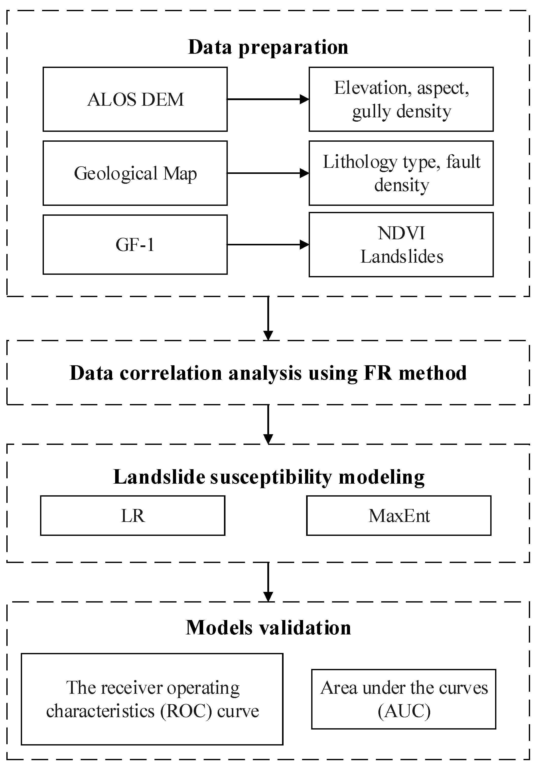
2. Materials and Methods

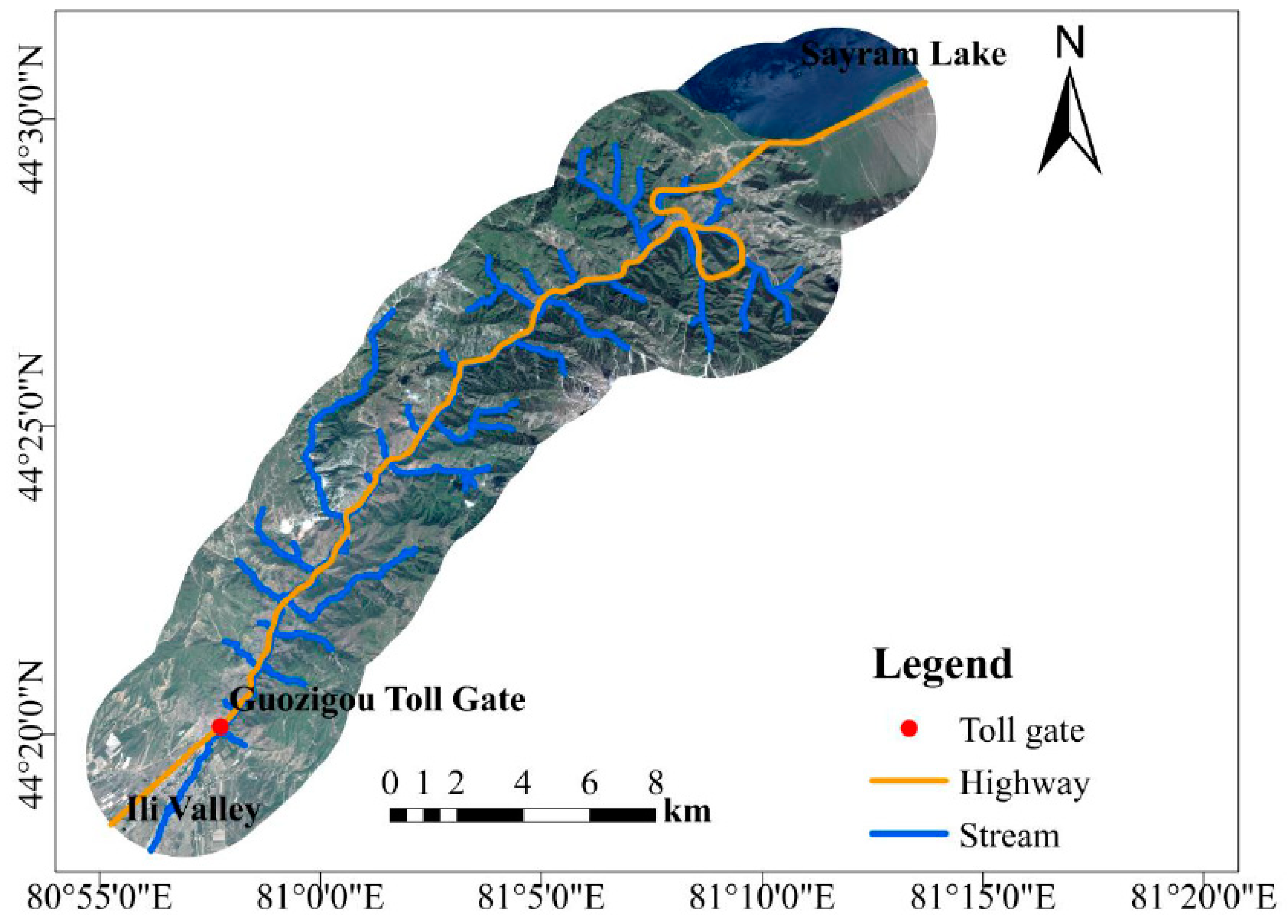
The following diagram shows the steps involved in the LSA in this research (Figure 1). There are four major steps. The first one is data preparation, including landslides inventory and conditioning factors. The second one is data correlation analysis through the frequency ratio, a bivariate statistical method. The third one is the landslide susceptibility modeling based on LR and MaxEnt methods. The final one is the models validation using the receiver operating characteristics (ROC) curve and area under the curves (AUC).

2.1. Study Area

The research area (44°18′N–44°31′N, 80°55′E–81°14′E) is a 3 km buffer of National Highway G30 in the Guozigou Valley, China, a steep, mountainous region where landslides occur frequently. It starts from Sayram Lake to the Guozigou toll gate and has a total length of 35 km (Figure 2). Guozigou Valley is a meandering valley across the Northern Tianshan Mountains in Xinjiang Uygur autonomous region, China. North of the valley is the Sayram Lake, and to the south lies the Ili Valley. It is the only way to reach the Ili Valley and also an important section of the ancient Silk Road. It has long been an essential passage to Central Asia and Europe. The highway G30 in Guozigou Valley plays a very important role in Xinjiang, China and even in Central Asia as an important highway corridor from the point of view of energy, material, economic, and cultural exchange, etc., especially under the strategy of the Belt and Road. It is considered as a “lifeline” for this region, but it faces frequent landslide events due to the extreme climate change in recent years, its geological stability having been damaged by human engineering activities and its own special geomorphological environment conditions [34,35]. Especially in May 2016, the heavy rain from 19:00 on 9 May 2016 caused landslides, and the collapse of roadbeds and retaining walls, and washed away the roadbed at K4161 + 000–K4196 + 720 (From Sayram Lake to Guozigou Toll station) G30 highway on 10 May 2016, which seriously affected the safety of vehicles and people. Landslides occur in a large number of places, blocking and damaging the road, and pose a severe threat to highway engineering, maintenance, and operation and even to people’s lives and properties, warranting our attention to the LSA in this area.

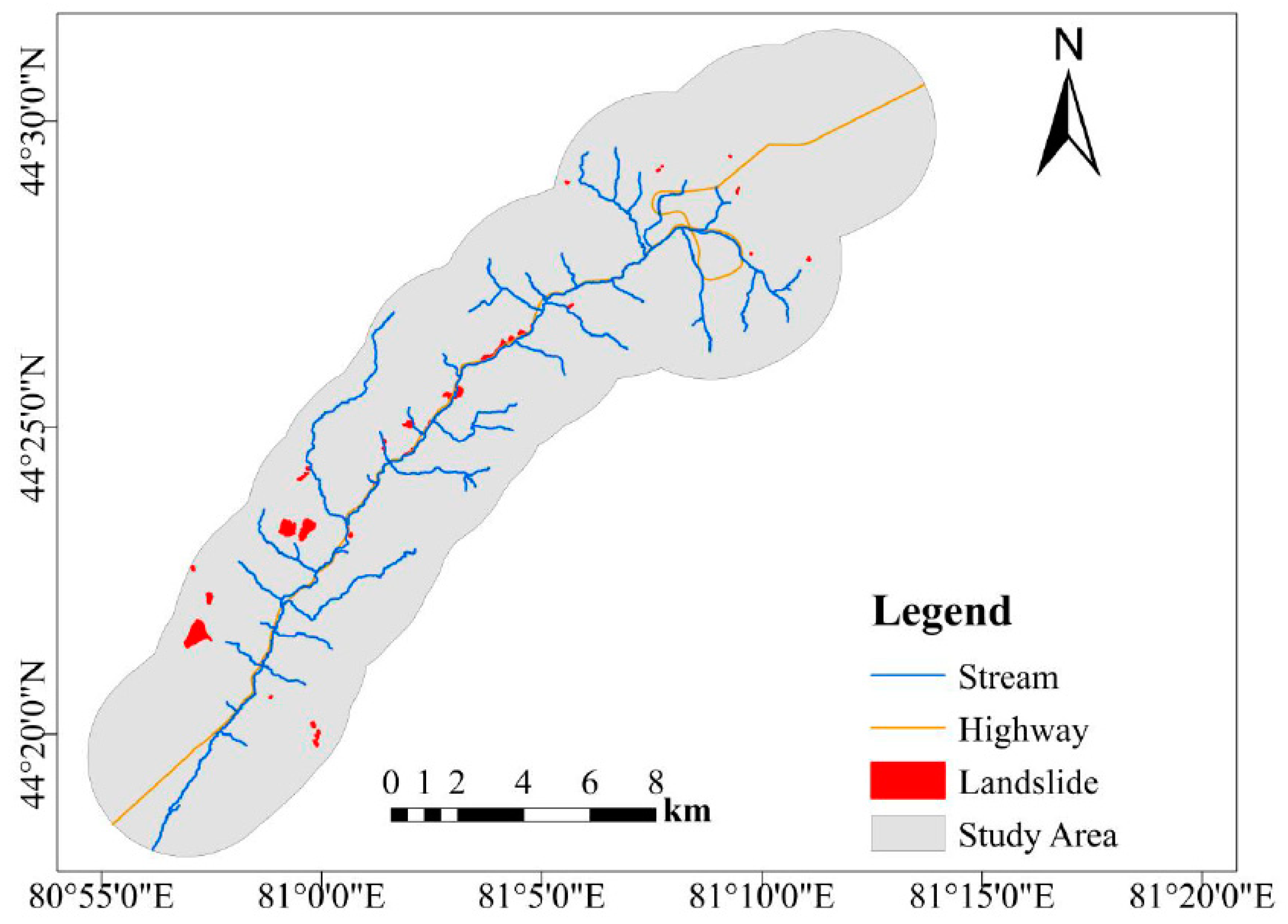
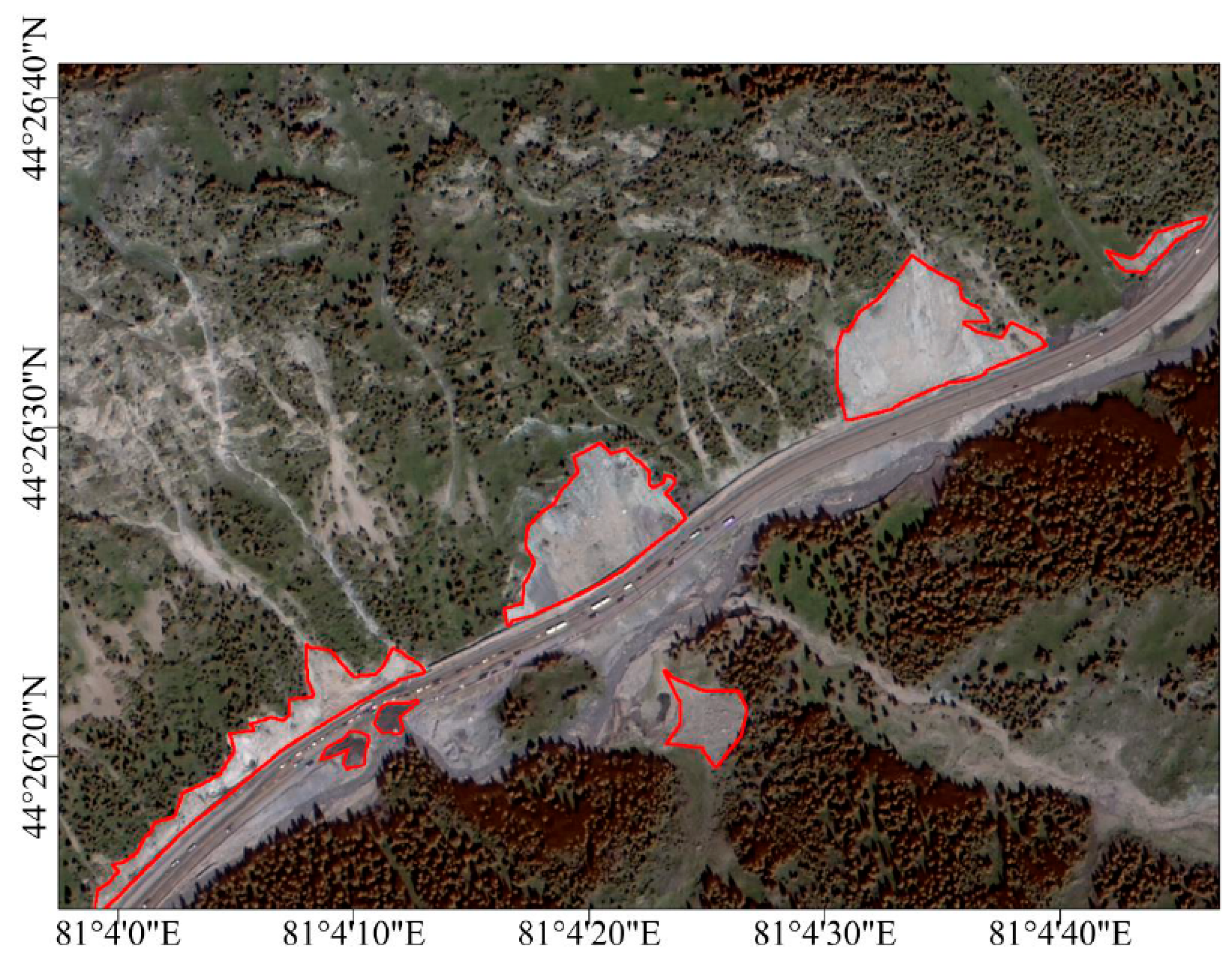
2.2. Landslide Inventory

Compiling landslide inventory is the crucial procedure of LSA [36]. The landslide inventory map shows the distribution and boundaries of landslides occurring in the landscape and provides important information for analyzing the relation of the landslide distributions to the conditioning factors, and for predicting the possibility of future landslides [37]. The landslide inventory in the current study was produced by the combination of the literature data, historical records, field surveys, Google Earth images, as well as data obtained through visual interpretation of GF-1 satellite data. GF is a series of Chinese civilian remote sensing satellites for the state-sponsored program China High-definition Earth Observation System (GF series, GF represents GaoFen, meaning “high resolution” in Chinese). GF-1 is an optical satellite with a 2 m resolution pan-chromatic camera, an 8 m resolution multi-spectral camera, and a 16 m resolution wide-angle multi-spectral camera. High spatial and temporal resolution remote sensing data can provide highly accurate information on ground features and enable the small-scale monitoring of highway geological hazards. Landslides can be distinguished from high-resolution satellite data based on their geomorphological characteristics, such as breaks in the bare soil and vegetated area, mass movement tracks, and appearance of flow materials in streams and gullies [13]. Field investigations were used to validate the previous landslide detected from GF-1 images and to find new landslides in the study region. Thirty-five historical landslides were identified along the highways in Guozigou Valley from 2002 to 2020 (Figure 3). Figure 4 shows the images of a few landslides along the highway in the study area. In this area, most landslides (in numbers) occurred along the highway (42.86%). The smallest and largest landslides were approximately 981.605 m² and 294,742 m², respectively. For landslide modeling, the centroid of the landslide polygon was extracted using ArcGIS 10.2 software packages from ESRI (Redlands, CA, USA) to present the landslide position. This can greatly simplify the landslide data, and it was also verified as practicable by many researchers [28]. Therefore, all landslides are represented in the form of points in this study, which makes the analysis easier.

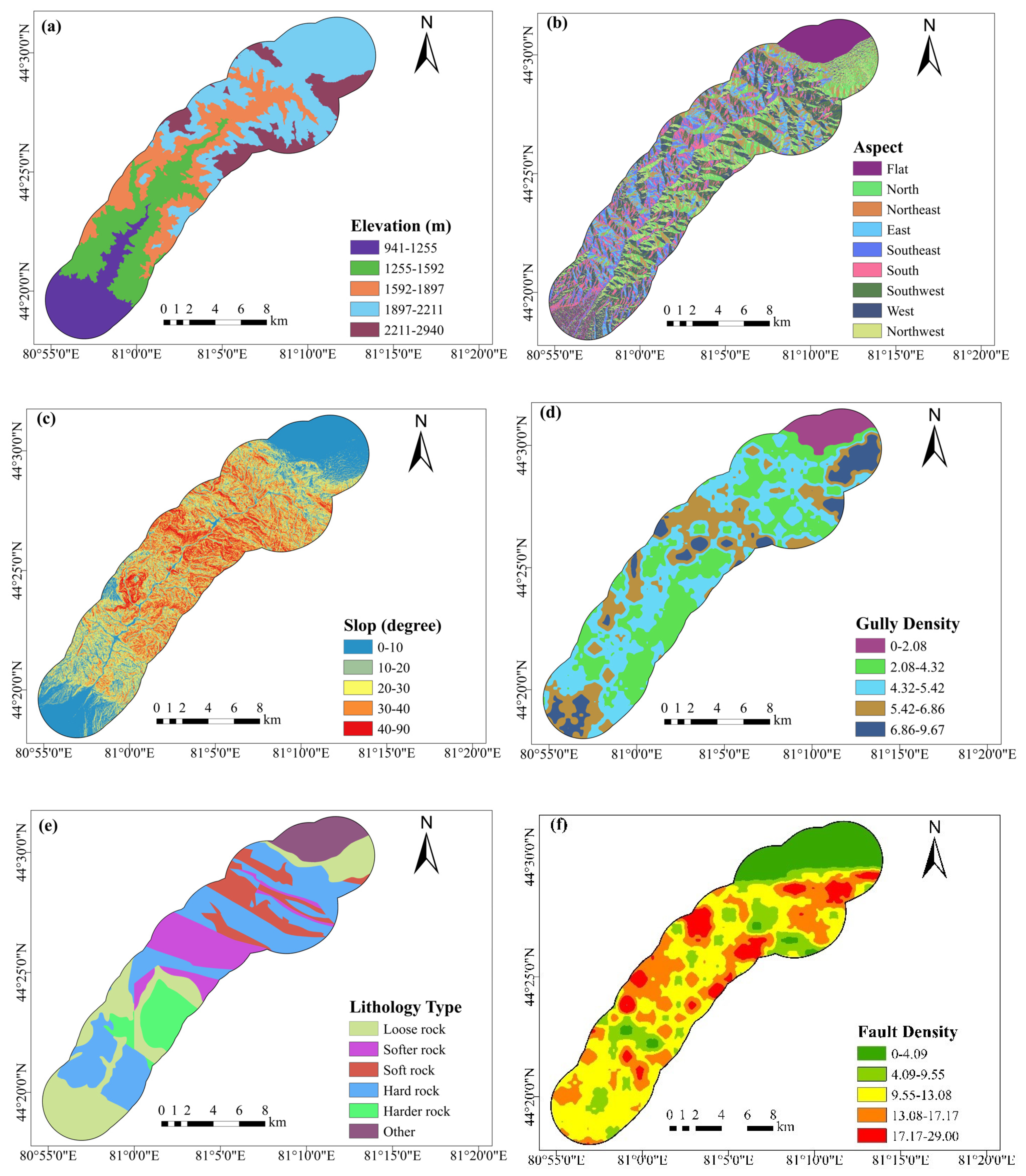
2.3. Landslide Conditioning Factors

Landslides are induced by a combination of numerous inter-related landslide conditioning factors (LCFs) and sometimes one can be more dominating than others [16]. Therefore, the selection and preparation of these LCFs to be considered as independent variables for the modeling is a vital procedure for the accuracy of the LSA model in determining landslide-susceptible regions [12]. However, there are no universal guidelines or set procedures to select LCFs. The selection of LCFs relies on the geological characteristics of the research region, the category of landslide, the main causes of landslide, the availability of data, the evaluation method, and the scale of the analysis [37]. The external and triggering factors such as earthquakes, precipitation, and erosion, etc. accelerate the frequency and speed of landslide disasters [38]. However, they were not considered in the current study because their data were not available in this study region.

In this study, seven LCFs (

Table 1. Data used in the study.

Conditioning Factors	Data Type	Source
Elevation	Continuous	Digital Elevation Model (DEM)
Aspect	Categorical (9 classes)	DEM
Slope	Continuous	DEM
Gully Density	Continuous	DEM
Lithology Type	Categorical (5 classes)	Geology Map
Fault Density	Continuous	Geology Map
NDVI	Continuous	GF-1 satellite image

) were selected for determining the landslide-susceptible zones in this study region including, elevation, slope, aspect, gully density, lithology, fault density, and normalized difference vegetation index (NDVI), which were chosen based on prior studies in the region of Guozigou Valley [34,35], the information collected from the literature [19,21], and field investigation. These variables are often applied in previous representative LSA. The data of slope, aspect, and gully density was extracted from the ALOS Palsar 12.5 m resolution Digital Elevation Model (DEM) in 2011. The data of lithology and faults was obtained through vectoring the 1:200,000 scale geological map, which was obtained from the reference room of the first regional geological survey brigade of Xinjiang Bureau of Geology and mineral resources. The NDVI is generated based on GF-1 satellite images (10 m resolution, acquired in July 2020 from the China Center for Resources Satellite Data and Application) using ENVI 5.3 software. Due to the different data types, coordinate systems, and description methods of the original data, all data were preprocessed using ArcGIS 10.2 in a unified way to achieve the purpose of factor classifications. Considering the calculation feasibility and accuracy, the vector layers were changed into raster layers having a 10 m × 10 m pixel size. The interpolation method of Inverse Distance Weighted (IDW) of the Spatial Analyst extension of ArcGIS 10.2 was used to resample the raster layer to 10 m resolution. Grid unit was used as a LSA unit. All factor data were projected to UTM coordinate system zone 44 with a WGS 84 Datum.

In this research, the LCFs have categorical (nominal) type, in which data has no natural order or ranking (e.g., aspect and lithology), and continuous (ordinal) type where the data has ranking and order (e.g., elevation, slope, gully density, fault density, and NDVI). The categorical factors were reclassified by manual methods based on previous research experience and literature data. The reclassification of continuous variables mainly used the Jenks Natural Breaks algorithm, which can determine the thresholds between categories of ordinal factors for the sake of maximizing the variance between classes and minimizing the variance inside of each class.

The relation of landslide occurrence to conditioning factors is described as follows. The landslide influencing factor maps are shown in Figure 5.

2.3.1. Elevation

Elevation is the height above sea level. It is one of the topographic factors which greatly influence the landslides occurrence [39]. It was applied in nearly all the LSA. It can be considered as an important factor in the LSA because it has direct impacts on the load-carrying capacity of the slope. In mountainous regions, external conditions, for instance, vegetation-growing conditions, rainfall, soil moisture, as well as human engineering activities are tightly associated with elevation. Moreover, the weathering profile also depends on the region elevation. In the current study, the elevation map was achieved through the classification of DEM. It varied from 941 m to 2940 m from sea level (Figure 5a).

2.3.2. Aspect

Aspect provides a description of the ground surface orientation that is surveyed clockwise in degrees from 0° (due north) to 360°. It is another important topographical factor in LSA. Aspect can affect many processes that have important impacts on the occurrence of landslides [40]. It affects rainfall infiltration and runoff, and the exposure to solar radiation that causes the moisture and vegetation distribution to be uneven. Usually, aspect has effects on the water content of soil. North-facing slopes usually have higher soil moisture and denser vegetation cover, which can protect greatly soil from shallow landslides and erosion [39], and most of the south-facing slopes lack vegetation or are sparsely vegetated, leading to swift mass erosion on moderate to abrupt slopes. Aspects in the study area were extracted from the DEM through the Aspect function of the ArcGIS 10.2 3D Analyst Toolbox and divided into nine classes comprising flat (−1), North (0°–22.5°; 337.5°–360°), Northeast (22.5°–67.5°), East (67.5°–112.5°), Southeast (112.5°–157.5°), South (157.5°–202.5°), Southwest (202.5°–247.5°), West (247.5°–292.5°), and Northwest (292.5°–337.5°), as in other studies (Figure 5b) [15,23].

2.3.3. Slope

Slope is generally believed to be an important topographical factor that has direct effects on landslide occurrence [39]. It was computed for each grid as the maximum elevation difference between the grid and its eight surroundings and extracted from DEM with the Slope function of the ArcGIS 10.2 3D Analyst Toolbox. Landslide occurrence increases along with the increase of slope. Usually, the slope will also impact the rainfall infiltration, the soil moisture, the shear stress distribution, and the movement processes of the landslide mass [39,41]. For this study, slope angle was within the ranges of 0 to 80.08° and the region lower than 30° accounted for over 70% of the study region, and the slope was divided into five categories with an equal intervals of 10° such as 0–10°, >10°–20°, >20°–30°, >30°–40°, and >40° (Figure 5c).

2.3.4. Gully Density

In the study, gully was represented by stream. Streams in the study area were extracted from the DEM through the hydrology function of the ArcGIS 10.2 Spatial Analyst Toolbox. The gully density was calculated to be the total length of stream in each grid area [34,35], which was also prepared through the ArcGIS Spatial Analyst tools. It was classified to 0–2.08 km/km², 2.08–4.32 km/km², 4.32–5.42 km/km², 5.42–6.86 km/km², and 6.86–9.67 km/km² using the natural breaks method (Figure 5d).

2.3.5. Lithology

Lithology (rock type) has an important effect on the landslides occurrence, especially in mountainous regions [21]. Various lithology indicates that the physical and geo-mechanical features of rocks are clearly different, including type, strength, density, permeability, anti-deformation ability, weathering degree, and durability [12]. In the current study, the lithology was obtained from a 1:200,000-scale geological map. To enhance the resolution of the lithology map, GF-1 satellite data (10 m spatial resolution) were employed to testify the lithology types through image enhancement techniques (band ratio combinations and principle component analysis) [17]. The lithology was classified into six classes including loose, softer, soft, hard, harder, and other (water) in the study area (Figure 5e) [42]. Granite and diorite were divided into the harder rock class; dolomite, limestone, and sand slate were divided into the hard rock class; mudstone, shale, phyllite, ophiolite, and fuelrock, etc. were divided into the softer rock class; quaternary unconsolidated sediments and extremely soft rocks with uniaxial compressive strength less than 5 MPa were divided into the loose rock class.

2.3.6. Fault Density

Faults play a significant role in the weakening of rock materials (reducing the strength of rock), which results in rock mass fracture and weathering, and causes landslides to occur [40]. In this study, the 1:200,000-scale geological map was employed to achieve the faults. Google Earth satellite images (<1 m resolutions) and GF-1 images (10 m resolution) were employed to testify and obtain other crucial faults that were not shown in the geologic map through the visual interpretation of satellite data [17]. The effect of faults is considered in the form of fault density in this study. Fault density is considered as an important indicative factor for landslide occurrence [43]. The fault density (km/km²) was computed from the fault polyline data through the ArcGIS Spatial Analyst tools. The fault density was expressed to be the total length of faults in each grid area. It was classified to 0–4.09 km/km², 4.09–9.55 km/km², 9.55–13.08 km/km², 13.08–17.17 km/km², and 17.17–29.00 km/km² using the natural breaks method (Figure 5f).

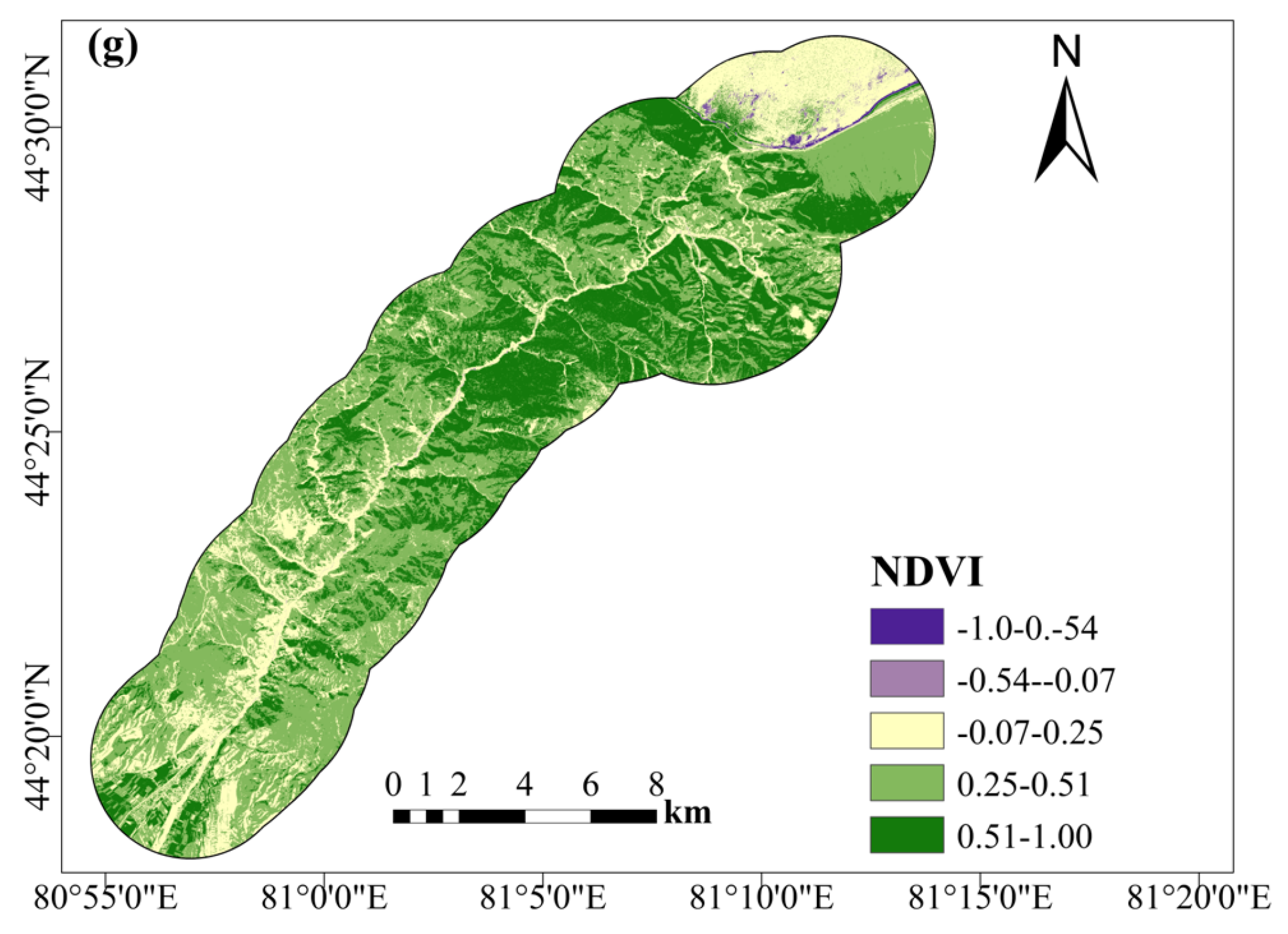
2.3.7. Normalized Difference Vegetation Index (NDVI)

The NDVI is one crucial factor quantifying the vegetation growth state and density, which affects the rainfall seepage, surface runoff, soil erosion, and rock weathering. Generally, the vegetation places a central part in immobilizing plenty of water and raising the shear strength and cohesion of soil [44]. Thus, NDVI was often thought to be an influencing factor in the LSA and was broadly employed in many studies [23]. The NDVI value varies from −1 to 1 in which negative one represents barren land and positive one indicates dense vegetated areas (Figure 5g). The larger the NDVI, the thicker the vegetation. The NDVI of this study was estimated using the GF-1 satellite data (acquired in July 2020) based on Equation (1):

$$\mathrm{NDVI}=\frac{(NIR-R)}{(NIR+R)}$$

(1)

where R and NIR represent the spectral reflectance measured in the near-infrared and visible (red) zones, respectively. For GF-1, NIR and R are band 5 (0.77–0.89 um) and band 4 (0.63–0.69 um).

2.4. Bivariate Method: Frequency Ratio

Building a model of landslide susceptibility requires certain knowledge of the relationship between the landslide distributions and the LCFs because it is commonly supposed that landslides will occur under similar conditions as in the past [9]. A GIS-based bivariate statistical method, the Frequency Ratio (FR), was applied to analyze the spatial relations between landslide distributions and LCFs individually and the effects of LCFs on the landslide occurrence [45]. The ${\mathrm{FR}}_i$ for each conditioning factor category is expressed as below [46]:

$${\mathrm{FR}}_i=(\frac{{\mathrm{N}}_{\mathit{ij}}}{{\mathrm{A}}_{\mathit{ij}}}/\frac{{\mathrm{N}}_{\mathrm{r}}}{{\mathrm{A}}_{\mathrm{r}}})$$

(2)

where ${\mathrm{N}}_{\mathit{ij}}$ is the pixel number of landslides in the study area related to the j-th category of i-th causative factor. ${\mathrm{A}}_{\mathit{ij}}$ is the number of pixels related to the j-th category of i-th causative factor. ${\mathrm{N}}_{\mathrm{r}}$ and ${\mathrm{A}}_{\mathrm{r}}$ are the total pixels of landslides and the study region. Therefore, it is obvious that $\frac{{\mathrm{N}}_{\mathit{ij}}}{{\mathrm{A}}_{\mathit{ij}}}$ shows the landslide density in a factor category (LD) and $\frac{{\mathrm{N}}_{\mathrm{r}}}{{\mathrm{A}}_{\mathrm{r}}}$ shows the landslide density in a causative factor.

A ${\mathrm{FR}}_i$ larger than 1 shows that the $i$th class of the factor under consideration is favorable for the occurrence of landslide. A ${\mathrm{FR}}_i$ less than 1 indicates that the $i$th class is not good for the occurrence of landslide [45]. If FR values of all classes of a factor were less than 1, then the factor was deleted from the potential factors. Generally, the greater the ${\mathrm{FR}}_i$ value, the higher the LOP under this factor, and vice versa [3].

2.5. Landslide Susceptibility Models

2.5.1. Logistic Regression

LR is frequently used for LSA because of its reliability [12,47]. LR is a linear multivariate regression analysis model which establishes the relationship between a dichotomous dependent variable Y, assigned the values 0 or 1 for ‘absence’ and ‘presence’ of landslides, and k independent variables (the conditioning factors), $x_1$, $x_2$,……, $x_k$, including categorical and continuous ones [6]. Compared with conventional linear regression methods, the LR method restrains the result value within the range of 0 and 1 using a logistic function, which is also called the sigmoid function. The LR predicts the LOP rather than directly predicting the landslide presence or absence [48]. Y is a Bernoulli distribution having the parameter $p_i=Pr(Y_i=1)$. So, $p_i$ is the probability of landslides occurrence for given values $x_1$, $x_2$,……, $x_k$ at location i [6]. In a LR, the expected value of $Y_i$ equals:

$$\mathrm{E}(Y_i)=\frac{1}{1+exp[-({\beta }_0+{\displaystyle {{\displaystyle \sum }}_{j=1}^k}{\beta }_j{x}_{ij})]}$$

(3)

The LR model applied to LSA for k independent variables was built as:

$$p_i=Pr(Y_i=1)=exp({\beta }_0+{\displaystyle {\sum }_{j=1}^k}{\beta }_j{x}_{ij})/[exp({\beta }_0+{\displaystyle {\sum }_{j=1}^k}{\beta }_j{x}_{ij})+1]$$

(4)

In LR, a Logit, namely, the natural logarithm of the odds, which is the ratio of the probability $P_i$ while $Y_i$ is 1 and the probability $1-P_i$ while $Y_i$ is 0, varies from −∞ to +∞ and is a linear regression function of the independent variables [47].

$$\mathrm{Logit}(P_i)=log(odds(P_i))=log(\frac{P_i}{1-P_i})={\beta }_0+{\displaystyle {\sum }_{j=1}^k}{\beta }_j{x}_{ij}$$

(5)

where, the βj, j = 0, …, k were regression coefficients that determine the importance of the independent variables to landslide occurrence, and $x_{ij}$ denotes the category of the jth conditioning factor at location i. The regression coefficients, ${\beta }_j$, were estimated by a maximum likelihood estimation (MLE). If the coefficient ${\beta }_j$ is positive, $e^{\beta }>$ 1, the factor is positively correlated with landslides; if β is negative, $e^{\beta }$ is within the range of 0 a 1. When $p_i$ is 1, it is suggested that landslides will certainly occur at this location, and when $p_i$ is 0, it is implicated that there is no landslide.

Both the data of landslide and nonlandslide points for training and verifying the LSA model were required. Nonlandslide data can greatly prevent statistical methods from overestimating landslide susceptibility [32]. However, landslide absence data cannot be directly obtained. In this study, the nonlandslide points were randomly generated in the landslide free area by ArcGIS 10.2, which is a frequently used method to produce landslide absence data for LSA [6]. Altogether, 135 points were selected, in which 100 points were nonlandslide and 35 points were landslide. Seven attributes of each point including all the selecting factors data were obtained through the Spatial Analyst Tools in ArcGIS 10.2.

In this study, the LR model was been created with the software SPSS 22.0 ^® (IBM). All the factors were taken as ordinal variables. In the model, the forward stepwise mode was used for considering the independent variables as in the literature [15].

2.5.2. MaxEnt

MaxEnt, as a generative presence-only machine-learning method, originates from information theory, and was initially put forward by Shannon [49,50]. MaxEnt was originally developed to predict the spatial pattern of species distribution [49]. It merely employs the presence positions of landslides and Gibbs distribution to calculate the landslide probability distribution function (PDF) by applying Bayes’ rule rather than using a discriminative strategy [49].

The presence-only characteristic of the model can be considered as an advantageous over other methods when the data are limited and in remote and inaccessible areas [49]. This characteristic is extremely crucial to landslide research because one cannot eliminate the probability that an area in the absence of landslide has high landslide occurrence potential. This method does not demand large amounts or high accuracy of investigation data; it can use both continuous and categorical variables, and it can also be employed to determine the importance of the conditioning factors without priori hypotheses [24].

This method was formulated according to the principle of maximum entropy, and ensures that the best approximation satisfies all the constraints on the unknown probability defined by the relation of the landslide occurrence data to their conditioning factors [26]. Thus, the best (optimum) landslide PDF selected for the unknown distribution ought to have maximum entropy (maximum quantity of information). The entropy formula based on the Boltzmann’s H-theorem can be defined as:

$$H(\widehat{\pi })=-{\displaystyle {\sum }_{xϵX}}\widehat{\pi }(x)\ln \widehat{\pi }(x)$$

(6)

where $\pi$ is the unknown landslide PDF on a finite group of pixels $x$ within the research region $X$; $\ln$ is the natural logarithm; and $\widehat{\pi }$ is the approximation of $\pi$. For each $x$, $\widehat{\pi }$ must have a non-negative probability value $P(x)$ to describe the LOP.

To estimate $P(x)$, a function $f_x$ is established to describe the information contained in the LCFs [49]:

$$f_x={\lambda }_1{f}_1+{\lambda }_2{f}_2+{\lambda }_3{f}_3+{\lambda }_4{f}_4+\cdots +{\lambda }_i{f}_i$$

(7)

where $f_i$ is the conditioning factor $i$, and ${\lambda }_i$ is a group of parameters. The probability of P(x) describes the maximum entropy distribution. The equation for maximum entropy distribution which belongs to the group of Gibbs’ distributions (exponential distributions) can be written as [24]:

$$P(x)=\frac{e^{f_x}}{Z_{\lambda }}$$

(8)

where $Z_{\lambda }$ is a normalized coefficient guaranteeing that the sum of probabilities $P(x)$ is one, and e is the mean of the function $f_x$ in the model of landslide occurrence, and can be expressed as

$$e=\frac{1}{m}{\displaystyle {\sum }_{i=1}^m}{f}_{xi}$$

(9)

The value of conditioning factor (E) of P must be extremely near to e. The constraint condition ($\ln Z_{\lambda }$) of P is |e − E| < β, where β is of any value.

$$\mathrm{E}={\displaystyle {\sum }_{x\in X}}P(x)f_x$$

(10)

$$\ln Z_{\lambda }=\frac{1}{m}{\displaystyle {\sum }_{i=1}^m}{f}_{xi}+{\displaystyle {\sum }_j}{\beta }_j{\lambda }_j$$

(11)

MaxEnt begins with a uniform PDF as a prior guess with the same probability for all pixels. Afterwards, a number of constraints enforce the uniform PDF to develop and produce a spatially optimized PDF of the landslide occurrence, which fulfills the constraints. This step begins with a random walk in the space of model parameters and obtains more precise results using an iterative procedure of learning/fitting and reassessing outputs.

MaxEnt software, version 3.4.1 [50], was used to study the relationship between landslides and its likely conditioning factors and to achieve LSA in our study. The locations of previous landslides were input as a dependent variable. The conditioning factors were input as independent variables. The data were in a 10 m grid format. The predefined defaults were selected for tuning parameters that were 1000 iterations, 10,000 random background locations (pseudo-absence locations), 0.5 as the initial prevalence value, 0.00001 as the convergent threshold, and the automatic feature selection strategy [24,26,33,49]. The model proceeded by fairly distinguishing the spatial distribution of landslides from that of the non-landslides and completely fitting on the training sites to ultimately provide a precise estimation of the landslide susceptibility in the calculation domain. The software was embedded with various data manipulation functions which considerably eased the modeling process. The primary result of MaxEnt was the LOP in each pixel that ranged from 0 to 1 [49,50]. These results could easily be imported into the GIS software. More mathematical details can be found in references [26,49].

2.6. Landslide Susceptibility Maps

Subsequently, the probability of the landslide occurrence was classified into four susceptibility levels containing low, moderate, high, and very high susceptibility zones, employing the natural breaks (Jenks) classification method in ArcGIS 10.2 to produce a landslide susceptibility map (LSM) [30]. The natural breaks (Jenks) classification method is a well-adapted selection to classify raster layers [12]. It has been successfully applied in various studies [30].

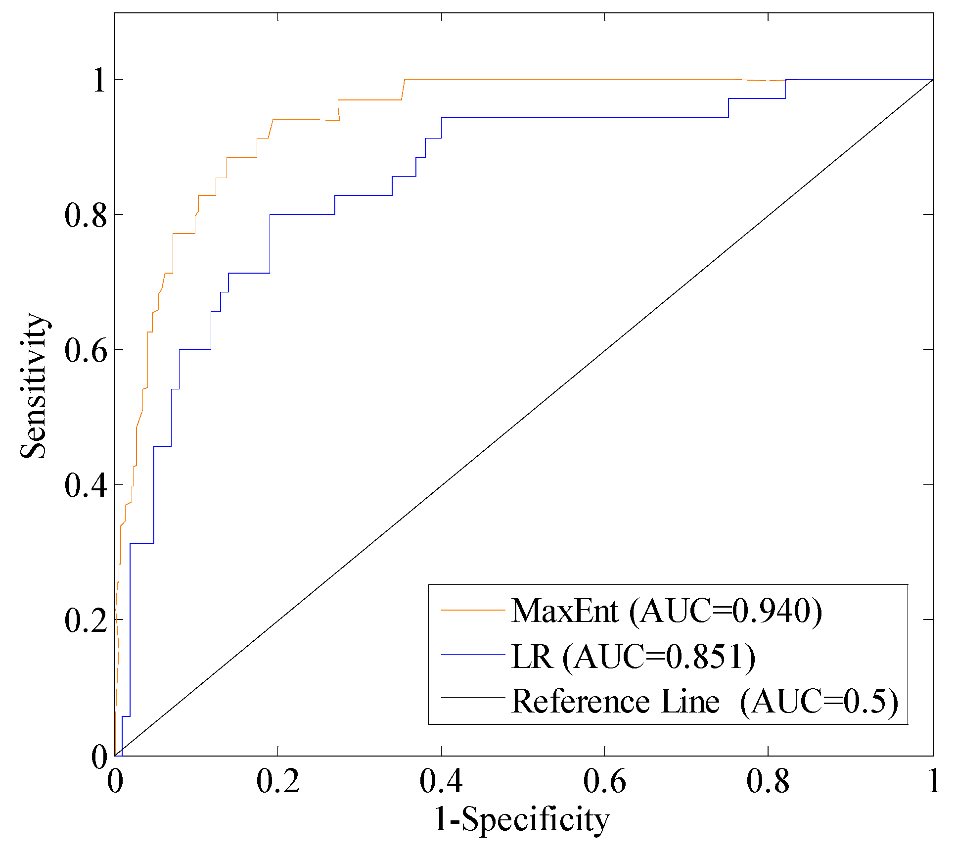
2.7. Model Performance

The ROC curve based on confusion matrices was applied to assess the prediction precision of the developed landslide susceptibility models [51]. The ROC curve, also called the success rate curve, compares the estimated probability with the real landslide distribution. It is the plot of the sensitivity (true positive rate) versus the 1-specificity (false positive rate) calculated for different susceptibility threshold values, and it was regarded as the statistic evaluation of the prediction capability of the model [20,51]. The value of the area under the curve (AUC) can quantitatively determine the accuracy of landslide model predictions [48]. It is one of the most useful accuracy statistics for LSA [48]. The value of AUC under the ROC curve changes from 0.5 (diagonals) to 1, which having a larger value shows the higher predictive power of the method [48]. The AUC value is divided into five categories: poor (0.5–0.6), moderate (0.6–0.7), good (0.7–0.8), very good (0.8–0.9) and excellent (0.9–1) predictive ability of the model [52]. In the current study, 35 landslides were employed to validate the two models results. Besides, percentage of landslide pixels on each susceptibility zones was computed to assess the model’s predictive precision.

3. Results

3.1. Bivariate Frequency Ratio

FR values of each category of the seven LCFs are presented in

Table 2. The area of landslides and frequency ratio (FR) value of each category for seven landslide-conditioning factors.

Conditioning Factors	Categories	Pixels of Land Area	Percentage of Domain (%)	Pixels of Landslide Area	Percentage of Landslides (%)	FR
Elevation (m)	941–1255	298,868	13.90	32	0.35	0.03
	1255–1592	418,538	19.47	7932	86.22	4.43
	1592–1897	458,777	21.34	1084	11.78	0.55
	1897–2211	749,941	34.89	137	1.49	0.04
	2211–2940	223,542	10.40	15	0.16	0.02
Aspect	Flat	174,720	8.13		0.00	0.00
	North	270,356	12.58	200	2.17	0.17
	Northeast	194,573	9.05	262	2.85	0.31
	East	199,082	9.26	1397	15.18	1.64
	Southeast	207,236	9.64	2627	28.55	2.96
	South	272,025	12.65	2974	32.33	2.55
	Southwest	293,547	13.66	792	8.61	0.63
	West	304,150	14.15	681	7.40	0.52
	Northwest	233,977	10.88	267	2.90	0.27
Slope	0–10	530,643	24.68	709	7.71	0.31
	10–20	481,847	22.41	2424	26.35	1.18
	20–30	506,654	23.57	2428	26.39	1.12
	30–40	386,096	17.96	1764	19.17	1.07
	40–90	244,426	11.37	1875	20.38	1.79
Gully Density	0–2.08	130,320	6.06		0.00	0.00
	2.08–4.32	636,067	29.59	2241	24.36	0.82
	4.32–5.42	767,112	35.68	3468	37.70	1.06
	5.42–6.86	437,781	20.36	2950	32.07	1.57
	6.86–9.67	178,517	8.30	541	5.88	0.71
Lithology Type	Loose Rock	531,449	24.72	3479	37.82	1.53
	Softer Rock	288,595	13.42	1749	19.01	1.42
	Soft Rock	227,049	10.56	73	0.79	0.08
	Hard Rock	764,054	35.54	3737	40.62	1.14
	Harder Rock	176,922	8.23	162	1.76	0.21
	Other	161,728	7.52		0.00	0.00
Fault Density	0–4.09	334,277	15.55	65	0.71	0.05
	4.09–9.55	279,183	12.99	1344	14.61	1.12
	9.55–13.08	843,030	39.21	3439	37.38	0.95
	13.08–17.17	530,926	24.70	4273	46.45	1.88
	17.17–29.00	162,380	7.55	79	0.86	0.11
NDVI	−1.00–0.54	6532	0.30		0.00	0.00
	−0.54–0.07	6671	0.31	28	0.30	0.98
	−0.07–0.25	433,388	20.16	6324	68.74	3.41
	0.25–0.51	1,040,774	48.41	2677	29.10	0.60
	0.51–1.00	662,432	30.81	171	1.86	0.06

. Seven factors had correlations with the occurrence of landslide because a FR value greater than 1 was shown in their class. When the slope was bigger than 20°, the FR value was higher than 1, which means slope greater than 20° had a positive correlation with landslides. In the slope categories of 0°–10°, 10°–20°, 20°–30°, 30°–40°, and 40°–90°, the FR values were 0.31, 1.18, 1.12, 1.07, and 1.79, respectively, and LD values, the ratio of landslide area in a category to the category area, were 0.13%, 0.50%, 0.48%, 0.46%, and 0.77%, respectively. The LOP was the largest in the elevation category of 1255–1592 m (FR = 4.43) with a LD of 1.90%. From the aspect FR results, it can be noticed that the LOP in the southeast direction was the largest because its FR value was 2.96, followed by the south direction (FR = 2.55) and the east direction (FR = 1.64). The FR values showed a positive correlation between the occurrence of landslide and slopes oriented to the southeast, south, and east, demonstrating the function of vegetation protection on slopes facing to the north. The LDs of the southeast, south, and east were 1.27%, 1.09%, and 0.70%, respectively. The gully density presented the largest FR value of 1.57 in the class of 5.42–6.86 km/km² with a LD of 0.67%. Concerning the lithology type, the loose rock, softer rock, and hard rock had FR values greater than 1 (1.53, 1.42, and 1.14, respectively) with a direct correlation with landslide occurrence and high LD (0.65%, 0.61%, and 0.49%, respectively). The ‘other’ class of the lithology type, the lake area, was not affected by the landslide. For fault density, the highest FR value of 1.88 was shown in the category of 13.08–17.17 km/km² with a LD of 0.80. The NDVI class of −0.54–0.07 presented the largest FR value of 3.41 and LD of 1.46, because the better the vegetation condition, the lower the LOP.

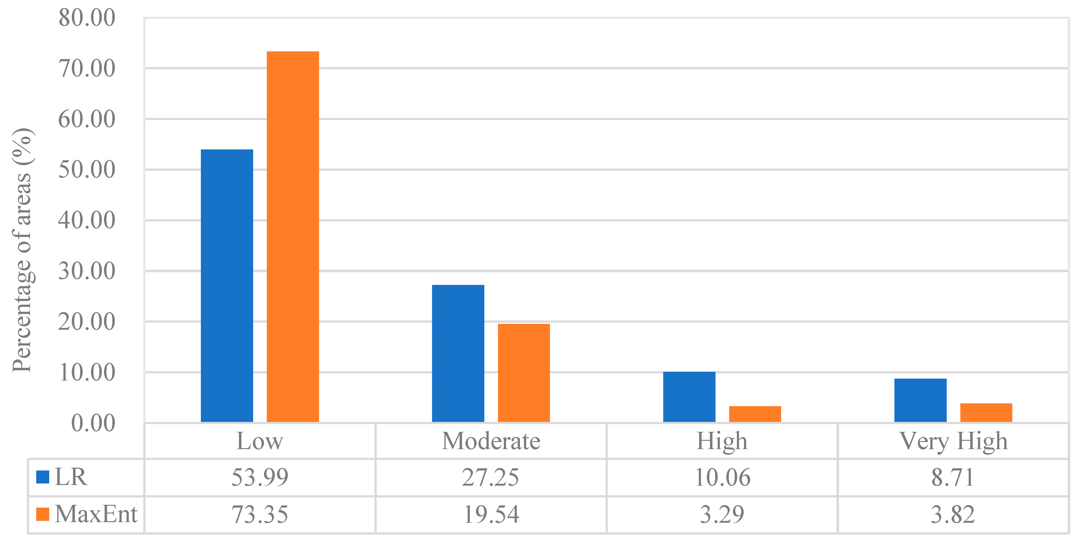
3.2. Logistic Regression

The Hosmer–Lemeshow test indicated that the goodness of fitting of the equation was acceptable because the Chi-square significance was greater than 0.05 and the overall accuracy percentage of the LR model was 82.2 (

Table 3. Summary of the logistic regression model.

−2 Log Likelihood	Cox and Snell R Square	Nagelkerke R Square	Overall Percentage
109.651 a	0.283	0.415	82.2

^a Estimation terminated at the fifth iteration, because the change of the estimated value of parameter was less than 0.001.

). The SPSS Binary Logistic procedures print the pseudo R² (Cox and Snell, and Nagelkerke) statistics, which had a similar meaning as the Regression R², but their values were less than 1. Nagelkerke (R²) is an adjusted version of the Cox and Snell (R²) that adjusts the statistic to range from 0 to 1. The values of Cox and Snell (R²) and Nagelkerke (R²) suggested that the dependent variable could be explained by the independent variables (Table 3).

Using the intercepts and coefficients achieved from the LR model, the logit formula was created as follows:

$$Y=3.931-1.868x_1+0.109x_2-0.272x_3-0.157x_4+0.444x_5+0.089x_6+0.285x_7$$

(12)

The obtained LR equation for calculating landslide probability for each pixel is as follows:

$$P=\frac{e^{3.931-1.868x_1+0.109x_2-0.272x_3-0.157x_4+0.444x_5+0.089x_6+0.285x_7}}{1+e^{3.931-1.868x_1+0.109x_2-0.272x_3-0.157x_4+0.444x_5+0.089x_6+0.285x_7}}$$

(13)

where, $x_1$ is the NDVI class, $x_2$ is the gully density class, $x_3$ is the elevation class, $x_4$ is the lithology type class, $x_5$ is the slope class, $x_6$ is the aspect class, and $x_7$ is the fault density class.

The established landslide susceptibility models were applied to estimate the LOP for every grid cell in entire study region through the Raster Calculator in ArcGIS 10.2. The LOP obtained from LR showed an average value of 0.167 over the whole study area, 0.503 in the landslide areas, and 0.166 in the non-landslide areas (

Table 4. The landslide occurrence probability within different regions.

Models	Study Region	Landslide Areas	Landslide-Free Areas
LR	0.167	0.503	0.166
MaxEnt	0.096	0.537	0.094

). Figure 5 shows the LSM of the study area generated using the LR model, which shows that the areas with low landslide susceptibility appeared as a sheet distribution, while the areas with very high landslide susceptibility showed a zonal distribution along the highway in Guozigou Valley. Most of the high-risk area could be noticed along highway G30 in the Guozigou Valley (Figure 6). The LSM achieved from LR indicated that more than 53% of the entire area was located in the low-susceptibility zones and 18.76% of the areas were located in the high- and very high- susceptibility areas (Figure 7). While overlaying the landslide inventory map with the LSM generated from the LR model, landslides were distributed mainly in the very high-susceptibility area and then in the moderate-, high-, and low-susceptibility areas (

Table 5. Percentage of landslide areas in each landslide susceptibility class.

Landslide Susceptibility Class	LR (%)	MaxEnt (%)
Low	7.85	7.27
Moderate	19.59	26.24
High	15.95	10.37
Very high	56.62	56.12

). Table 5 shows the area percentage of landslides in different landslide susceptibility areas.

The ROC curve for the LR model is presented in Figure 8. The AUC value of the LR model was 0.851, which presented an accuracy of 85.1% for the built LR model. The standard error of the ROC curve was 0.038 and the asymptotic eigenvalue was smaller than 0.05, which is within the specified bounds (

Table 6. Area under the curve (AUC) values of the models.

Models	Area	Standard Error	Asymptotic Significant	Asymptotic 95% Confidence Interval
				Lower Limit	Upper Limit
LR	0.851	0.038	0.000	0.776	0.926
MaxEnt	0.940	0.031	0.000	0.844	0.956

). This indicates the model had high accuracy and the susceptibility map would be reliable along highway G30 in the Guozigou Valley.

3.3. MaxEnt

The LOP obtained from the MaxEnt model showed an average value of 0.096 in the whole study area, 0.537 in the landslide areas, and 0.094 in the landslide-free areas (Table 4). In the entire study area, the average LOP of the LR model was larger than that of MaxEnt model, but in the landslide areas, that of the MaxEnt model was larger than that of the LR model (Table 4). This indicates, to some extent, the overestimation problem of the LR model and the better predication ability of the MaxEnt model.

The patterns of spatial distribution of the LSM produced by the two models had a similarity in that the very high landslide susceptibility areas were mostly distributed along highway G30 in the Guozigou Valley (Figure 6). The low susceptibility-to-landslide class, using LR and MaxEnt models, had the highest areal percentage, exceeding 53% of the study region (Figure 7), but the area percentage of landslides in this susceptibility zone was less than 10% (Table 5). The very high-susceptibility class using the two models basically occupied the lowest areal distribution, smaller than 10% of the study region, but a noticeably large percentage (more than 56%) of the landslide areas occurred in this class (Figure 7, Table 5). It is generally believed that a model has a better landslide prediction performance if actual landslides are mainly distributed in high- and very high-susceptibility zones generated by the model [29]. The statistical results indicated that the two susceptibility maps are reliable and reasonable.

In addition, comparing the LSM produced by the two models with the landslide inventory map, it can be seen that a very high-susceptibility area generated by LR was in the south region of the study area (Figure 3 and Figure 6a); however, actually, there have been few past landslides in that region. LR overestimated landslide occurrence in the south region. In the results of MaxEnt, this overestimation of landslides in the south region was not obvious (Figure 3 and Figure 6b). This result also indicated that the ability of landslide prediction of the MaxEnt model is superior to that of the LR.

The ROC curve (Figure 8) was also applied to assess the prediction performance of the MaxEnt method. It can be noticed that the AUC values of both methods were above 0.8, which demonstrates that the two methods had good prediction abilities. The MaxEnt method was superior to the LR model, as it had the larger AUC value (AUC = 0.940), which shows the excellent predictive ability of the MaxEnt model. Compared with the conventional statistical methods, MaxEnt produced more robust and reliable results and eased the problems of misclassification [17].

4. Discussion

4.1. Causes of Landslide along Highway in Mountainous Area

In this study, the very high-susceptibility class was mainly distributed along the highway in Guozigou Valley. Landslides occurring along highways in mountainous areas are a common situation [29]. This result is similar to those of many previous studies. For instance, the landslide material volume from roadside slopes was 65,470 m³/km², which is 30 times that of natural forest regions in the western Cascade Range, Oregon [53]. Extremely high rates of surface erosion and landslides were noticed after the building of Weixi–Shangri road (23.5 km) in Yunan province, China, which were averaged up to 9600 t ha⁻¹ [54]. The region around the highways was confirmed to be the most prone to landslides in the Andes of southern Ecuador [55], where landslide occurrence was noticed to be more than one order of magnitude higher within a close distance of the built intercity highways compared with long distances [56].

There is an interaction between road construction and landslide disasters in mountainous areas. Road construction (escarpment roads) in mountainous regions involves engineering activities, for instance, cutting, excavating, or blasting slopes, resulting in altered geological and topographical conditions of the original slopes, and the subsequent destruction of the slope’s original stability, leading to slope instability [44]. In addition, due to road-relevant construction and deforestation activities, the construction of roads interrupts surface drainage, changes groundwater movement, alters mass distribution, and accelerates erosion [10,54]. It is well known that mountain roads increase the occurrence of landslides because of the imperfect drainage systems and the mechanical instability of hillslopes resulting from undercutting and overloading [44,56].

Therefore, it was an essential step to perform LSA along the mountainous highway, the landslide-prone area, to improve the safety of transportation, and reduce the maintenance cost of the highways and the loss of life and properties. Suitable areas for developmental activities can be identified by determining safe locations with low landslide susceptibility [57]. High-susceptibility zones should be avoided as much as possible, as these areas mostly consist of unstable slopes that may be susceptible to failure.

4.2. Comparison of LR and MaxEnt

There are many elements influencing the accuracy of LSA, such as reliability of raw data (e.g., landslide data), selection of conditioning factors, resolution of DEM, sampling sizes and strategies, evaluation units, the ratio between presence and absence data, and the performances of classification models [15,23,58]. Here, the predictive abilities of the model were focused on.

The model comparison enables us to better evaluate advantages and limitations of each model as well as the reliability of statistics. The predictive ability of two methods was compared in our study using AUC. The MaxEnt model, with an excellent AUC value of 0.940, exhibited excellent predictive ability versus the LR with a very good AUC value of 0.851, which is similar to the conclusion of other relevant comparative studies. MaxEnt was a high-performance prediction model for the LSM of the Boeun area in Korea and the prediction performance of MaxEnt was slightly better than that of the LR model [25]. The precision of the Shannon entropy method is higher than that of the LR and the conditional probability theory models at the road section of Mugling-Narayanghat in the Nepal Himalayas [40]. The precision of the maximum entropy method is higher than the LR and the tree regression methods in the lower part of the Deba Valley (Guipúzcoa province, Spain) [33]. MaxEnt showed the maximum AUC value (0.812) for the LSA of the Taleghan basin, Iran, compared with FR, LR, and SVM [57].

There are reports that the performance of MaxEnt was better than other models. The index of entropy model with an AUC of 86.08% was slightly superior to the conditional probability model with an AUC of 82.75% at Safarood basin, Iran [59]. The results accuracy of the LSM of the Index of Entropy (IoE) model were higher than those of the Dempster–Shafer (DS) model for the Sarkhoun catchment, Southwestern Iran [60]. The MaxEnt produces the best results for LSA of the Honghe Hani Rice Terraces, a World Heritage site located in Yuanyang County, Southwest China, followed by the mean distance (Domain) model, the information value model (IVM), and biological climatic (Bioclim) model [61]. The physically based model presented an accuracy of 65.9% in terms of the AUC; however, the ensemble maximum entropy-based machine learning algorithm showed a higher accuracy of 79.6% and a predictive rate of 89.7% in Mt. Umyeon, South Korea [62].

The MaxEnt model presented an excellent prediction ability for landslides in Golestan Province, Northeast Iran, with an AUROC value of 0.889 [63]. The MaxEnt model not only performed well in the degree of fitting, but also achieved remarkable results in multi-hazard (including floods, landslides, and gullies erosion) predictive performance in Gorganrood Watershed, Golestan Province (Iran) [64]. The SVM and MaxEnt models can provide more stable and robust results and are less sensitive to the input data changes and, therefore, are more reliable in the Chehel-Chai Watershed, Golestan Province, Northern Iran [65].

In contrast, the LR model showed the best landslide predictive ability in the LSM in Ganzhou City for the AUC values of the data-driven LR, Maxent, FR, and evidential belief function (EBF) models were 0.8237, 0.7903, 0.7789, and 0.7367, respectively [43]. The AUC of FR model was slightly higher than that of index of entropy model for success and prediction rate in the Al-Hasher area, Jizan, Kingdom of Saudi Arabia [19]. For LSA, maximum entropy (ME) was inferior to support vector machine with the radial basis function kernel (SVM-RBF) in predictive performance with the respective values of 0.84 and 0.887 for the most important cities in Gorganrood Basin, Iran [66]. ANN achieved the maximum AUC with a value of 0.824, followed by SVM with a value of 0.819, and MaxEnt with a value of 0.75 in the Wanyuan area, China [30]. These opposite conclusions may be due to various reasons: through examples, the differences of regional geographical environments, the factors considered in the selection of indicators, and the amount of data used for the construction of the models, among others. Hence, in the process of model selection, there is no one model that performs best for every problem.

There are some disadvantages in the two methods. The LR method is not very suitable for unbalanced data where the non-landslide observations (pixels) are much greater than the landslide observations [16]. Reclassifying continuous data for conventional statistical methods is necessary, and it implies a subjective selection of the ranges chosen for each study zone [23]. LR has some problems concerning the quasi-complete classification of categorical variables changed into dummy explanatory variables [15]. The presence-only property of MaxEnt, apart from its advantages, especially avoiding further inspection of the landslide-free locations, may make the model face more biased data, especially when the landslide data are often found near the accessible roads and passable locations [30]. In addition, the generated pseudo-absence data should be applied with great caution in MaxEnt as they directly influence the model results, and trustworthy pseudo-absence data are not always available [67]. One of the other shortcomings of MaxEnt and LR is that they use landslide inventory by only including the landslide point features and ignoring the landslide shape and size information.

In summary, the two models are very fast and extremely easy to use, which is the biggest advantage in LSA models; the MaxEnt, as a generative presence-only model, provides better predictive results using very few training data, compared with LR; this may be due to LSM being considered as a predictive modeling with presence-only data, because most available information is on previous landslide locations in most cases.

5. Conclusions

Landslides occur frequently along the highway G30 in Guozigou Valley, just as in the other roads in the mountainous region, which causes road disruption, blocking, etc., and even severely endangers the lives and properties of people.

Based on FR values, high-susceptibility positions in this study region are caused by the negative synergy effect of slopes of greater than 20°, elevations of 1255–1592 m, southeast-facing slopes, gully densities of 5.42–6.86 km/km², loose rocks, fault densities of 13.08–17.17 km/km², and NDVI values of −0.54–0.07.

In the present work, we implemented the multivariate statistical LR and generative presence-only MaxEnt for LSA along the G30 highway in Guozigou valley by the aid of GF-1 satellite data and GIS techniques. The spatial distribution patterns of the LSM produced by the LR and MaxEnt methods had a similarity in that the highly landslide-prone regions were distributed mostly along the highway in the Guozigou Valley. Landslides were distributed mainly in the very high-susceptibility areas through comparing the produced LSM with the actual landslide occurrences, which showed that the two LSMs were reliable and reasonable. In addition, the AUC value of the LR and the MaxEnt model was 0.851 and 0.940, respectively. It could be noticed that the AUC values of both methods were higher than 0.8, which demonstrates that the two methods have better prediction performances. Therefore, it may be concluded that the two methods can be applied in LSA in the research area. However, LR showed, to some extent, an overestimation problem and overestimated landslide occurrence in the south region. Both the ROC curve and the AUC values showed that the MaxEnt model had better performance in LSA in this area. Compared with the conventional statistical model (LR), MaxEnt produced more reliable and robust results. Moreover, for most cases, the most available data are past landslide occurrences; therefore, the generative presence-only MaxEnt model is more suitable to LSA. The MaxEnt model could be used in data-scarce regions such as rugged mountain areas in future studies.

The results of the LSA of the study area would provide reference for decision-makers, planners, and engineers to make wise decisions about land-use planning and disaster prevention and mitigation in the upcoming years. The areas with very high landslide susceptibility along the highway should be completely surveyed on site, and appropriate measures should performed. Detailed local surveys are also needed in the future for better evaluation and analysis of the development characteristics of landslide geological disasters in the study area. In addition, the external and triggering factors such as earthquakes, precipitation, and erosion, etc. should be considered in the LSA in future detailed studies.

References

1. Das, I.; Stein, A.; Kerle, N.; Dadhwal, V.K. Landslide susceptibility mapping along road corridors in the Indian Himalayas using Bayesian logistic regression models. Geomorphology 2012, 179, 116–125. [Google Scholar] [CrossRef]
2. Raja, N.B.; Çiçek, I.; Türkoğlu, N.; Aydin, O.; Kawasaki, A. Landslide susceptibility mapping of the Sera River basin using logistic regression model. Nat. Hazards 2017, 85, 1323–1346. [Google Scholar] [CrossRef] [Green Version]
3. Choi, J.; Oh, H.J.; Lee, H.J.; Lee, C.; Lee, S. Combining landslide susceptibility maps obtained from frequency ratio, logistic regression, and artificial neural network models using ASTER images and GIS. Eng. Geol. 2012, 124, 12–23. [Google Scholar] [CrossRef]
4. Kaczmarek, Ł.D.; Popielski, P. Selected components of geological structures and numerical modelling of slope stability. Open Geosci. 2019, 11, 208–218. [Google Scholar] [CrossRef]
5. Dai, F.C.; Lee, C.F.; Ngai, Y.Y. Landslide risk assessment and management: An overview. Eng. Geol. 2002, 64, 65–87. [Google Scholar] [CrossRef]
6. Das, I.; Sahoo, S.; Van Westen, C.J.; Stein, A.; Hack, R. Landslide susceptibility assessment using logistic regression and its comparison with a rock mass classification system, along a road section in the northern Himalayas (India). Geomorphology 2010, 114, 627–637. [Google Scholar] [CrossRef]
7. Goetz, J.N.; Guthrie, R.H.; Brenning, A. Integrating physical and empirical landslide susceptibility models using generalized additive models. Geomorphology 2011, 129, 376–386. [Google Scholar] [CrossRef]
8. Strauch, R.L.; Raymond, C.L.; Rochefort, R.M.; Hamlet, A.F.; Lauver, C. Adapting transportation to climate change on federal lands in Washington State, U.S.A. Clim. Chang. 2015, 130, 185–199. [Google Scholar] [CrossRef]
9. Van Westen, C.J.; van Asch, T.W.J.; Soeters, R. Landslide hazard and risk zonation—Why is it still so difficult? Bull. Eng. Geol. Env. 2006, 65, 167–184. [Google Scholar] [CrossRef]
10. Banerjee, P.; Ghose, M.K. Spatial analysis of environmental impacts of highway projects with special emphasis on mountainous area: An overview. Impact Assess. Proj. Apprais. 2016, 34, 279–293. [Google Scholar] [CrossRef] [Green Version]
11. Corominas, J.; Moya, J. A review of assessing landslide frequency for hazard zoning purposes. Eng. Geol. 2008, 102, 193–213. [Google Scholar] [CrossRef]
12. Ayalew, L.; Yamagishi, H. The application of GIS-based logistic regression for landslide susceptibility mapping in the Kakuda-Yahiko Mountains, Central Japan. Geomorphology 2005, 65, 15–31. [Google Scholar] [CrossRef]
13. Lee, S. Application of logistic regression model and its validation for landslide susceptibility mapping using GIS and remote sensing data. Int. J. Remote Sens. 2005, 26, 1477–1491. [Google Scholar] [CrossRef]
14. Shahabi, H.; Hashim, M.; Ahmad, B.B. Remote sensing and GIS-based landslide susceptibility mapping using frequency ratio, logistic regression, and fuzzy logic methods at the central Zab basin, Iran. Environ. Earth Sci. 2015, 73, 8647. [Google Scholar] [CrossRef]
15. Trigila, A.; Iadanza, C.; Esposito, C.; Scarascia-Mugnozza, G. Comparison of logistic regression and random forests techniques for shallow landslide susceptibility assessment in Giampilieri (NE Sicily, Italy). Geomorphology 2015, 249, 119–136. [Google Scholar] [CrossRef]
16. Reichenbach, P.; Rossi, M.; Malamud, B.D.; Mihir, M.; Guzzetti, F. A review of statistically based landslide susceptibility models. Earth-Sci. Rev. 2018, 180, 60–91. [Google Scholar] [CrossRef]
17. Youssef, A.M.; Pourghasemi, H.R. Landslide susceptibility mapping using machine learning algorithms and comparison of their performance at Abha Basin, Asir Region, Saudi Arabia. Geosci. Front. 2021, 12, 639–655. [Google Scholar] [CrossRef]
18. Yalcin, A. GIS-based landslide susceptibility mapping using analytical hierarchy process and bivariate statistics in Ardesen (Turkey): Comparisons of results and confirmations. Catena 2008, 72, 1–12. [Google Scholar] [CrossRef]
19. Youssef, A.M.; Al-Kathery, M.; Pradhan, B. Landslide susceptibility mapping at Al-Hasher Area, Jizan (Saudi Arabia) using GIS-based frequency ratio and index of entropy models. Geosci. J. 2015, 19, 113–134. [Google Scholar] [CrossRef]
20. Lee, S.; Ryu, J.H.; Won, J.S.; Park, H.J. Determination and application of the weights for landslide susceptibility mapping using an artificial neural network. Eng. Geol. 2004, 71, 289–302. [Google Scholar] [CrossRef]
21. Tien Bui, D.; Tuan, T.A.; Klempe, H.; Pradhan, B.; Revhaug, I. Spatial prediction models for shallow landslide hazards: A comparative assessment of the efficacy of support vector machines, artificial neural networks, kernel logistic regression, and logistic model tree. Landslides 2016, 13, 361–378. [Google Scholar] [CrossRef]
22. Huang, Y.; Zhao, L. Review on landslide susceptibility mapping using support vector machines. Catena 2018, 165, 520–529. [Google Scholar] [CrossRef]
23. Chen, W.; Zhang, S.; Li, R.W.; Shahabi, H. Performance evaluation of the GIS-based data mining techniques of best-first decision tree, random forest, and naïve Bayes tree for landslide susceptibility modeling. Sci. Total Environ. 2018, 644, 1006–1018. [Google Scholar] [CrossRef]
24. Convertino, M.; Troccoli, A.; Catani, F. Detecting fingerprints of landslide drivers: A MaxEnt model. J. Geophys. Res. Earth Surf. 2013, 118, 1367–1386. [Google Scholar] [CrossRef] [Green Version]
25. Park, N.W. Using maximum entropy modeling for landslide susceptibility mapping with multiple geoenvironmental data sets. Environ. Earth Sci. 2015, 73, 937–949. [Google Scholar] [CrossRef]
26. Kornejady, A.; Ownegh, M.; Bahremand, A. Landslide susceptibility assessment using maximum entropy model with two different data sampling methods. Catena 2017, 152, 144–162. [Google Scholar] [CrossRef]
27. Ngo, P.T.T.; Panahi, M.; Khosravi, K.; Ghorbanzadeh, O.; Kariminejad, N.; Cerda, A.; Lee, S. Evaluation of deep learning algorithms for national scale landslide susceptibility mapping of Iran. Geosci. Front. 2021, 12, 505–519. [Google Scholar] [CrossRef]
28. Pham, B.T.; Nguyen-Thoi, T.; Qi, C.; Phong, T.V.; Dou, J.; Ho, L.S.; Le, H.V.; Prakash, I. Coupling RBF neural network with ensemble learning techniques for landslide susceptibility mapping. Catena 2020, 195, 104805. [Google Scholar] [CrossRef]
29. Zhou, X.Z.; Wen, H.J.; Zhang, Y.L.; Xu, J.H.; Zhang, W.G. Landslide susceptibility mapping using hybrid random forest with GeoDetector and RFE for factor optimization. Geosci. Front. 2021, 12, 101211. [Google Scholar] [CrossRef]
30. Chen, W.; Pourghasemi, H.R.; Kornejady, A.; Zhang, N. Landslide spatial modelling: Introducing new ensembles of ANN, MaxEnt, and SVM machine learning techniques. Geoderma 2017, 305, 314–327. [Google Scholar] [CrossRef]
31. Dehnavi, A.; Aghdam, I.N.; Pradhan, B.; Varzandeh, M.H.M. A new hybrid model using step-wise weight assessment ratio analysis (SWARA) technique and adaptive neuro-fuzzy inference system (ANFIS) for regional landslide hazard assessment in Iran. Catena 2015, 135, 122–148. [Google Scholar] [CrossRef]
32. Zhu, A.X.; Miao, Y.M.; Yang, L.; Bai, S.B.; Liu, J.Z.; Hong, H.Y. Comparison of the presence-only method and presence-absence method in landslide susceptibility mapping. Catena 2018, 171, 222–233. [Google Scholar] [CrossRef]
33. Felicísimo, Á.M.; Cuartero, A.; Remondo, J.; Quirós, E. Mapping landslide susceptibility with logistic regression, multiple adaptive regression splines, classification and regression trees, and maximum entropy methods: A comparative study. Landslides 2012, 10, 175–189. [Google Scholar] [CrossRef]
34. Zhao, L.J.; Li, H.; Liu, Y.F.; Chen, D.H.; Li, J.L. Evaluation on geological hazard risk and disaster-causing factors in the Guozigou Valley in Ili, Xinjiang. Arid. Zone Res. 2017, 34, 693–700. [Google Scholar]
35. Zhao, L.J.; Chen, D.H.; Li, H.; Liu, Y.F. A method to assess landslide susceptibility by using logistic regression model for Guozigou Region, Xinjinag. Mt. Res. 2017, 32, 203–211. [Google Scholar]
36. Guzzetti, F.; Carrara, A.; Cardinali, M.; Reichenbach, P. Landslide hazard evaluation: A review of current techniques and their application in a multiscale study, Central Italy. Geomorphology 1999, 31, 181–216. [Google Scholar] [CrossRef]
37. Guzzetti, F.; Mondini, A.C.; Cardinali, M.; Fiorucci, F.; Santangelo, M.; Chang, K.T. Landslide inventory maps: New tools for an old problem. Earth-Sci. Rev. 2012, 112, 42–66. [Google Scholar] [CrossRef] [Green Version]
38. Tanyas, H.; van Westen, C.J.; Persello, C.; Alvioli, M. Rapid prediction of the magnitude scale of landslide events triggered by an earthquake. Landslides 2019, 16, 661–676. [Google Scholar] [CrossRef] [Green Version]
39. Dai, F.C.; Lee, C.F. Landslide characteristics and slope instability modelling using GIS, Lantau Island, Hong Kong. Geomorphology 2002, 42, 213–228. [Google Scholar] [CrossRef]
40. Devkota, K.C.; Regmi, A.D.; Pourghasemi, H.R.; Yoshida, K.; Pradhan, B.; Ryu, I.C.; Dhital, M.R.; Althuwaynee, O.F. Landslide susceptibility mapping using certainty factor, index of entropy and logistic regression models in GIS and their comparison at Mugling-Narayanghat road section in Nepal Himalaya. Nat. Hazards 2013, 65, 135–165. [Google Scholar] [CrossRef]
41. Hong, H.; Naghibi, S.A.; Pourghasemi, H.R.; Pradhan, B. GIS-based landslide spatial modeling in Ganzhou City, China. Arab. J. Geosci. 2016, 9, 112. [Google Scholar] [CrossRef]
42. Yang, J.T.; Song, C.; Yang, Y.; Xu, C.D.; Guo, F.; Xie, L. New method for landslide susceptibility mapping supported by spatial logistic regression and GeoDetector: A case study of Duwen Highway Basin, Sichuan Province, China. Geomorphology 2019, 324, 62–71. [Google Scholar] [CrossRef]
43. Kawabata, D.; Bandibas, J. Landslide susceptibility mapping using geological data, a DEM from ASTER images and an Artificial Neural Network (ANN). Geomorphology 2009, 113, 97–109. [Google Scholar] [CrossRef]
44. Sidle, R.C.; Ochiai, H. Landslides: Processes, Prediction, and Land Use; American Geophysical Union: Washington, DC, USA, 2006. [Google Scholar]
45. Lee, S.; Min, K. Statistical analysis of landslide susceptibility at Yongin, Korea. Environ. Geol. 2001, 40, 1095–1113. [Google Scholar] [CrossRef]
46. He, Y.; Beighley, E. GIS-based regional landslide susceptibility mapping: A case study in southern California. Earth Surf. Proc. Land. 2008, 33, 380–393. [Google Scholar] [CrossRef]
47. Van Den Eeckhaut, M.; Vanwalleghem, T.; Poesen, J.; Govers, G.; Verstraeten, G.; Vandekerckhove, L. Prediction of landslide susceptibility using rare events logistic regression: A case-study in the Flemish Ardennes (Belgium). Geomorphology 2006, 76, 392–410. [Google Scholar] [CrossRef]
48. Brenning, A. Spatial prediction models for landslide hazards: Review, comparison and evaluation. Nat. Hazards Earth Syst. Sci. 2005, 5, 853–862. [Google Scholar] [CrossRef]
49. Phillips, S.J.; Anderson, R.P.; Schapire, R.E. Maximum entropy modeling of species geographic distributions. Ecol. Model. 2006, 190, 231–259. [Google Scholar] [CrossRef] [Green Version]
50. Phillips, S.J.; Dudík, M.; Schapire, R.E. Maxent Software for Modeling Species Niches and Distributions (Version 3.4.1). 2021. Available online: http://biodiversityinformatics.amnh.org/open_source/maxent/ (accessed on 25 July 2021).
51. Beguería, S. Validation and evaluation of predictive models in hazard and risk assessment. Nat. Hazards 2006, 37, 315–329. [Google Scholar] [CrossRef] [Green Version]
52. Wang, Y.M.; Feng, L.W.; Li, S.J.; Ren, F.; Du, Q.Y. A hybrid model considering spatial heterogeneity for landslide susceptibility mapping in Zhejiang Province, China. Catena 2020, 188, 104425. [Google Scholar] [CrossRef]
53. Swanson, F.J. Impact of clear-cutting and road construction on soil erosion by landslides in the western Cascade Range, Oregon. Geology 1975, 3, 393–396. [Google Scholar] [CrossRef]
54. Sidle, R.C.; Furuichi, T.; Kono, Y. Unprecedented rates of landslide and surface erosion along a newly constructed road in Yunnan, China. Nat. Hazards 2011, 57, 313–326. [Google Scholar] [CrossRef]
55. Muenchow, J.; Brenning, A.; Richter, M. Geomorphic process rates of landslides along a humidity gradient in the tropical Andes. Geomorphology 2012, 139, 271–284. [Google Scholar] [CrossRef]
56. Brenning, A.; Schwinn, M.; Ruiz-Páez, A.P.; Muenchow, J. Landslide susceptibility near highways is increased by 1 order of magnitude in the Andes of southern Ecuador, Loja province. Nat. Hazards Earth Syst. Sci. 2015, 15, 45–57. [Google Scholar] [CrossRef] [Green Version]
57. Mokhtari, M.; Abedian, S. Spatial prediction of landslide susceptibility in Taleghan basin, Iran. Stoch. Environ. Res. Risk Assess. 2019, 33, 1297–1325. [Google Scholar] [CrossRef]
58. Pourghasemi, H.R.; Kornejady, A.; Kerle, N.; Shabani, F. Investigating the effects of different landslide positioning techniques, landslide partitioning approaches, and presence-absence balances on landslide susceptibility mapping. Catena 2020, 187, 104364. [Google Scholar] [CrossRef]
59. Pourghasemi, H.R.; Mohammady, M.; Pradhan, B. Landslide susceptibility mapping using index of entropy and conditional probability models in GIS: Safarood Basin, Iran. Catena 2012, 97, 71–84. [Google Scholar] [CrossRef]
60. Shirani, K.; Pasandi, M.; Arabameri, A. Landslide susceptibility assessment by Dempster–Shafer and Index of Entropy models, Sarkhoun basin, Southwestern Iran. Nat. Hazards 2018, 93, 1379–1418. [Google Scholar] [CrossRef]
61. Jiao, Y.M.; Zhao, D.M.; Ding, Y.P.; Liu, Y.; Xu, Q.; Qiu, Y.M.; Liu, C.J.; Liu, Z.L.; Zha, Z.Q.; Li, R. Performance evaluation for four Gis-based models purposed to predict and map landslide susceptibility: A case study at a World Heritage site in Southwest China. Catena 2019, 183, 104221. [Google Scholar] [CrossRef]
62. Pradhan, A.; Kang, H.S.; Lee, J.S.; Kim, Y.T. An ensemble landslide hazard model incorporating rainfall threshold for Mt. Umyeon, South Korea. Bull. Eng. Geol. Environ. 2019, 78, 131–146. [Google Scholar] [CrossRef]
63. Sheikh, V.; Kornejady, A.; Ownegh, M. Application of the coupled TOPSIS–Mahalanobis distance for multi-hazard-based management of the target districts of the Golestan Province, Iran. Nat. Hazards 2019, 96, 1335–1365. [Google Scholar] [CrossRef]
64. Javidan, N.; Kavian, A.; Pourghasemi, H.R.; Conoscenti, C.; Jafarian, Z.; Rodrigo-Comino, J. Evaluation of multi-hazard map produced using MaxEnt machine learning technique. Sci. Rep. 2021, 11, 6496. [Google Scholar] [CrossRef] [PubMed]
65. Teimouri, M.; Kornejady, A. The dilemma of determining the superiority of data mining models: Optimal sampling balance and end users’ perspectives matter. Bull. Eng. Geol. Environ. 2019, 79, 1707–1720. [Google Scholar] [CrossRef]
66. Mirzaei, G.; Soltani, A.; Soltani, M.; Darabi, M. An integrated data-mining and multi-criteria decision-making approach for hazard-based object ranking with a focus on landslides and floods. Environ. Earth Sci. 2018, 77, 581. [Google Scholar] [CrossRef]
67. Phillips, S.J.; Dudık, M.; Elith, J.; Graham, C.H.; Lehmann, A.; Leathwick, J.; Ferrier, S. Sample selection bias and presence-only distribution models: Implications for background and pseudo-absence data. Ecol. Appl. 2009, 19, 181–197. [Google Scholar] [CrossRef] [PubMed] [Green Version]
Figure 1. A diagram of the research steps of this study.
Remotesensing 14 03620 g001
Figure 2. Location map of the study area where the background is the GF-1 satellite bands 1, 2, and 3 true-color composed image acquired in July 2020.
Remotesensing 14 03620 g002
Figure 3. Landslide inventory map for 2020, generated mainly using GF-1 satellite images.
Remotesensing 14 03620 g003
Figure 4. Chinese GF-2 bands 1, 2, and 3 true-color composed image of landslides with red outline which occurred along the highway in the Guozigou Valley on 13 May 2016 after heavy rainfall on 10 May 2016.
Remotesensing 14 03620 g004
Figure 5. Causative factors of landslides: (a) elevation, (b) aspect, (c) slope, (d) gulley density, (e) lithology type, (f) fault density, and (g) NDVI.
Remotesensing 14 03620 g005aRemotesensing 14 03620 g005b
Figure 6. Landslide susceptibility maps generated applying the (a) LR and (b) MaxEnt models.
Remotesensing 14 03620 g006
Figure 7. Area percentage of different landslide susceptibility zones within the research region using the models.
Remotesensing 14 03620 g007
Figure 8. ROC curves of the models.
Remotesensing 14 03620 g008