KASiam: Keypoints-Aligned Siamese Network for the Completion of Partial TLS Point Clouds

Abstract

Completing point clouds from partial terrestrial laser scannings (TLS) is a fundamental step for many 3D visual applications, such as remote sensing, digital city and autonomous driving. However, existing methods mainly followed an ordinary auto-encoder architecture with only partial point clouds as inputs, and adopted K-Nearest Neighbors (KNN) operations to extract local geometric features, which takes insufficient advantage of input point clouds and has limited ability to extract features from long-range geometric relationships, respectively. In this paper, we propose a keypoints-aligned siamese (KASiam) network for the completion of partial TLS point clouds. The network follows a novel siamese auto-encoder architecture, to learn prior geometric information of complete shapes by aligning keypoints of complete-partial pairs during the stage of training. Moreover, we propose two essential blocks cross-attention perception (CAP) and self-attention augment (SAA), which replace KNN operations with attention mechanisms and are able to establish long-range geometric relationships among points by selecting neighborhoods adaptively at the global level. Experiments are conducted on widely used benchmarks and several TLS data, which demonstrate that our method outperforms other state-of-the-art methods by a 4.72% reduction of the average Chamfer Distance of categories in PCN dataset at least, and can generate finer shapes of point clouds on partial TLS data.

1. Introduction

In recent years, with the rapid development and wide application of LiDARs, point clouds have become the main data format for 3D scene understanding and have been playing an important role in the areas of remote sensing, robotics, digital city and so on [1]. However, raw scanning point clouds from LiDARs are not always satisfactory and complete, as they are often sparse and partial because of inappropriate scanning factors such as light refraction, occlusion and limitation of sensor resolution. Therefore, predicting missing regions from their partial scannings is uniquely significant to many downstream applications.

Benefiting from the emergence of large-scale point cloud datasets and the improvement of computer technology, researchers have tried many approaches to tackle the issue of point cloud completion by the way of deep learning, which can be divided into three categories: Voxel-based methods, MLP-based (Multilayer Perception) methods and Attention-based methods. In the Voxel-based methods, 3D-EPN [2] maps voxelized 3D shapes into a probabilistic latent space and completes single objects by 3D convolution operations. GRNet [3] takes 3D grids as intermediate representations to complete point clouds. VE-PCN [4] embeds point clouds into regular voxel grids and then generates complete point clouds with the aid of shape edges. In the MLP-based methods, PCN [5] uses tandem layers of PointNet [6] to extract shape features of partial point clouds. TopNet [7] proposes a tree decoder that generates structured point clouds. NSFA [8] explores and aggregates multi-level features to represent known parts and missing parts separately. CRN [9] proposes a cascaded refinement network to generate detailed object shapes by a coarse-to-fine strategy. In the Attention-based methods, SnowflakeNet [10] applies a transformer-based [11] point deconvolution structure to the decoding process. PoinTr [12] regards the completion process as a translation issue and proposes a transformer-based auto-encoder structure for point cloud completion. Most of the above methods have two common techniques. Firstly, they follow an ordinary auto-encoder architecture with only partial point clouds as inputs. Secondly, they apply K-Nearest Neighbors (KNN) operations or their variant (e.g., ball query operations) on feature extractions, to explore the local geometric relationships among points.

However, the ordinary auto-encoder network with embedded KNN blocks is not the most effective method for point cloud completion. Firstly, the ordinary auto-encoder network with only partial point clouds as inputs only uses complete point clouds as references for calculating the loss function, and takes insufficient advantage of their intrinsic geometric features. Secondly, KNN is unable to extract geometric semantic features effectively at local incomplete regions of partial input point clouds and needs a trade-off between efficiency and accuracy. To tackle these issues, ASFM-Net [13] employs an asymmetrical siamese feature matching strategy to map the partial and complete input point cloud into a shared latent space. VRCNet [14] proposes a dual-path architecture to enable principled probabilistic modelling across partial and complete point clouds. However, these two methods only use 3D position coordinates of each point for position embedding, and fail to depict local geometries of points explicitly. SnowflakeNet [10] and PoinTr [12] adopt attention mechanisms to explore long-range geometric relationships among points. Global-KNN [15] improves KNN and selects neighborhoods of points adaptively by calculating attention weights. However, these methods still use the Euclidean distance as measurement without breaking the limit of KNN operations.

In this paper, we propose a keypoints-aligned siamese (KASiam) network to solve the above issues for the completion of partial TLS point clouds. KASiam has dual input-asymmetric paths, which are the reconstruction path with complete point clouds as inputs and the completion path with partial point clouds as inputs, respectively. Both paths are linked to each other through keypoints alignment operations. Each path has a similar pipeline, which consists of a feature extractor, a keypoint generator and two shape refiners. Moreover, we propose two essential blocks cross-attention perception (CAP) and self-attention augment (SAA) in the pipeline, which replace KNN operations with attention mechanisms, and are able to select neighborhoods adaptively to establish long-range geometric relationships among points. We compare KASiam with various state-of-the-art methods on the widely used benchmark PCN dataset [5] and several TLS data scanned by a RigelScan LiDAR. Experimental results and analyses demonstrate that our method has achieved leading performance on point clouds completion. Our main contributions can be summarized as follows:

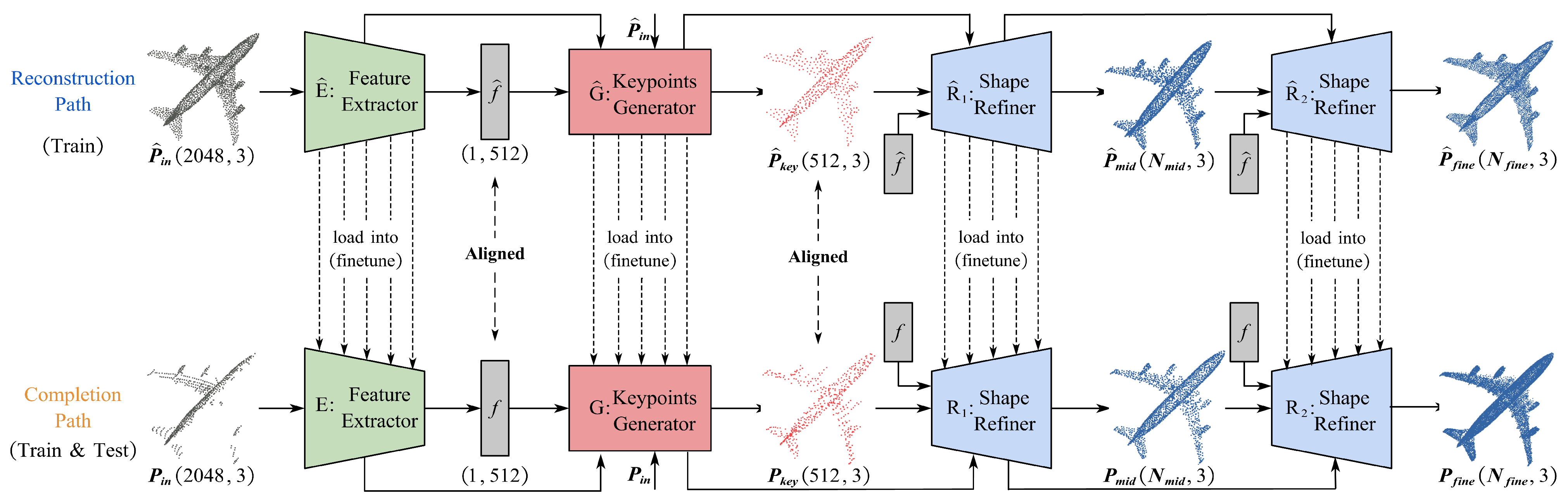
• We propose the KASiam network for point cloud completion. KASiam has dual input paths of reconstruction and completion, which interact geometric features with each other through keypoints alignment of complete-partial pairs. The dual path structure takes sufficient advantage of input data and is crucial for the completion task.
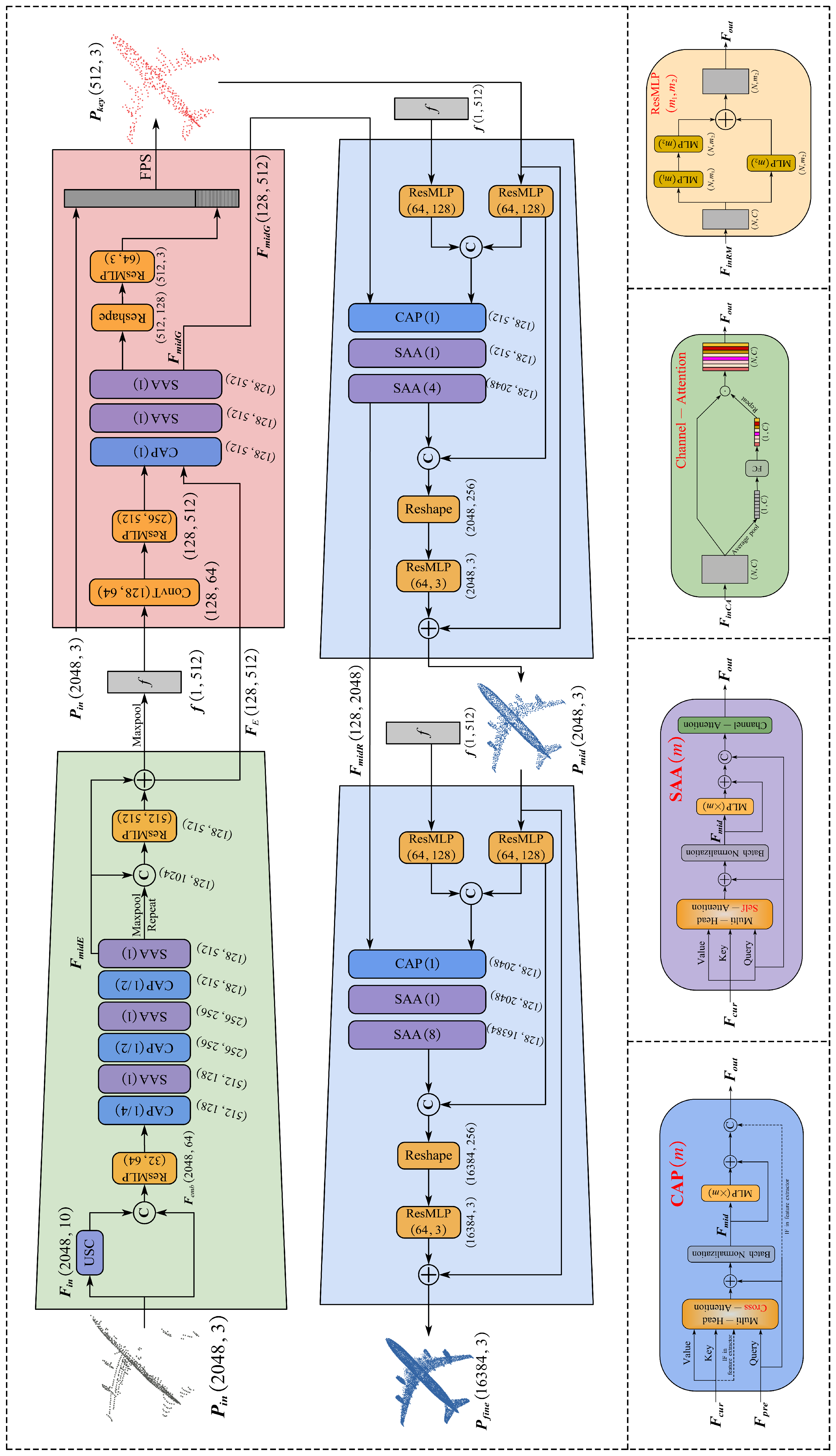
• We propose CAP and SAA blocks, which weaken the explicit local feature extractions and replace KNN with per-point attention mechanisms, to make the network able to learn geometric relationships precisely in an implicit manner.
• Experimental results and analyses demonstrate that KASiam achieves the state-of-the-art point cloud completion performance, outperforms existing methods by at least a 4.72% reduction of the average Chamfer Distance of categories in PCN dataset especially and can generate finer shapes of point clouds on partial TLS data.

2. Related Work

This section can be divided into three parts: Section 2.1 is a summary of point clouds features exploitations, which are fundamental tools for most of the point cloud analyses and understanding of tasks based on deep learning. Section 2.2 surveys three types of point cloud completion methods by focusing on different structures of networks. Section 2.3 is a summary of evaluations on point cloud completion, some of which are utilized by KASiam.

2.1. Point Cloud Features Exploitation

MLP-based methods. PointNet [6] is a pioneer of point cloud analysis by deep learning, which models every point independently by MLPs and uses a symmetric function to handle the order invariance of point clouds. PointNet++ [16] proposes two sets of abstraction layers to extract local geometric features. PointMLP [17] builds a deeper network through a pure residual MLP structure to explore high-dimensional geometric features. Inspired by triangle meshes and umbrella curvature in computer graphics, RepSurf [18] computes geometric representations of point clouds by predefined geometric priors after surface reconstruction. Convolution-based methods. Because of the unstructured nature of point clouds, convolution operations cannot be directly applied to them. Thus, PointCNN [19], PointConv [20], PAConv [21] and FSDCNet [22] extract features of point clouds through self-defined convolution kernels. DGCNN [23], AGConv [24] and GACM [25] search neighborhoods of key points by graph convolutions [26]. Transformer-based methods, inspired by the success of Transformers in 2D image processing [27,28], PCT [29], PT [30] and Pointformer [31], model geometric relationships between points by calculating attention weight matrices.

2.2. Point Cloud Completion

Voxel-based methods. The 3D-EPN method [2] completes partial shapes while using semantic context from a shape classification network by 3D convolutions, and matches output shapes with 3D geometries in existing shape datasets. GRNet [3] proposes two novel differentiable blocks named gridding block and gridding reverse block, to generate point clouds by grids without losing structural information. VE-PCN [4] incorporates object structure features into the completion process by leveraging edge generation, and proposes a multi-scale voxel-based network to predict finer shapes. However, due to the quantization effect of 3D voxel representation, most voxel-based methods meet a trade-off between efficiency and accuracy [7], and may not be suitable for practical applications.

MLP-based methods. PCN [5] is a pioneer of point cloud completion by MLP layers. It encodes geometric features through two tandem layers of PointNet [6], and generates complete shapes by a manifold fitting network FoldingNet [32]. TopNet [7] proposes a hierarchical decoder to predict structured point clouds and publishes a new dataset Completion3D. NSFA [8] models missing parts and complete parts respectively to predict the whole point cloud shapes. CRN [9] considers local details of partial inputs with global shape information together, to preserve the existing details and generate missing parts. However, most of these methods follow an ordinary auto-encoder architecture with only partial point clouds as inputs, and may make insufficient use of the intrinsic geometric features of inputs.

Attention-based methods. With applications of transformer structures in point clouds [29,30,31], attention relationships between points are increasingly considered in the point cloud completion task. SA-Net [33] proposes a skip-attention mechanism to effectively explore local structure details of partial point clouds during the inference of missing shapes. VRCNet [14] designs a point selective kernel module to exploit and fuse multi-scale point features effectively by self-attention operations. SnowflakeNet [10] applies a transformer-based point deconvolution structure to interpret the generation process of complete point cloud into an explicit and locally structured pattern. PoinTr [12] is a pioneer of using pure transformer structures in the completion task, and regards the completion process as a translation of point sets. Global-KNN [15] proposes an adaptive neighborhood feature extraction module to select neighborhoods of keypoints adaptively according to different target shapes. However, most of these methods apply KNN operations or its variant to select neighborhoods of points by the Euclidean distance measurement, and ignore long-distance semantic relationships between points.

Other methods. SoftPoolNet [34] proposes a new module named soft pooling to replace the max-pooling operation in PointNet [6] by taking into account multiple high-score features rather than just the highest. PMP-Net [35] proposes a novel network to mimic the behaviour of an earth mover. It generates complete point clouds by moving every point in incomplete inputs to ensure the shortest total distance of all point moving paths. PF-Net [36] and SpareNet [37] introduce the method of Generative Adversarial Networks (GAN) [38] into the point cloud completion task.

2.3. Evaluation on Point Cloud Completion

For 3D point cloud completion, Chamfer Distance (CD) and Earth Mover’s Distance (EMD) are the most frequently used performance criteria [39]. CD represents the average distance of the closest point between two point clouds. EMD aims to find out a bijection to minimize the average distance between corresponding points from partial and complete ones [40]. In recent years, many works have expanded the CD criteria. MPED [41] measures point clouds geometry and color difference by a distortion quantification of multi-scale potential energy discrepancy. DCD [42] is derived from CD and it can detect the disparity of density distributions.

3. Method

3.1. Overall Architecture

The overall architecture of KASiam is shown in Figure 1, which adopts a siamese auto-encoder structure for point cloud completion. KASiam has dual input-asymmetric paths, which are the reconstruction path with complete point clouds as inputs and the completion path with partial point clouds as inputs, respectively. Both paths are linked to each other through keypoints alignment operations (Section 3.6). Each path has a similar pipeline, which consists of three modules: a feature extractor (Section 3.2), a keypoint generator (Section 3.3) and two shape refiners (Section 3.4). The operation process of KASiam is as follows. In the training phase, we first train the reconstruction path with complete point clouds as inputs to explore features of complete shapes and generate skeleton keypoints. Then, we load the pre-trained model into the completion path to finetune for fitting the feature distribution of complete point clouds and predicting the position of skeleton key points of missing regions. In the testing phase, we abandon the reconstruction path and only use the completion path to generate complete point clouds, which ensures fairness in comparison with other methods without importing additional information. For clarity, we add symbols $\widehat{}$ to the variables and modules on the reconstruction path. Because the two paths of KASiam share the same structure, we take the completion path for example in Section 3.2–Section 3.5, and the details of the network can be seen in Appendix A.

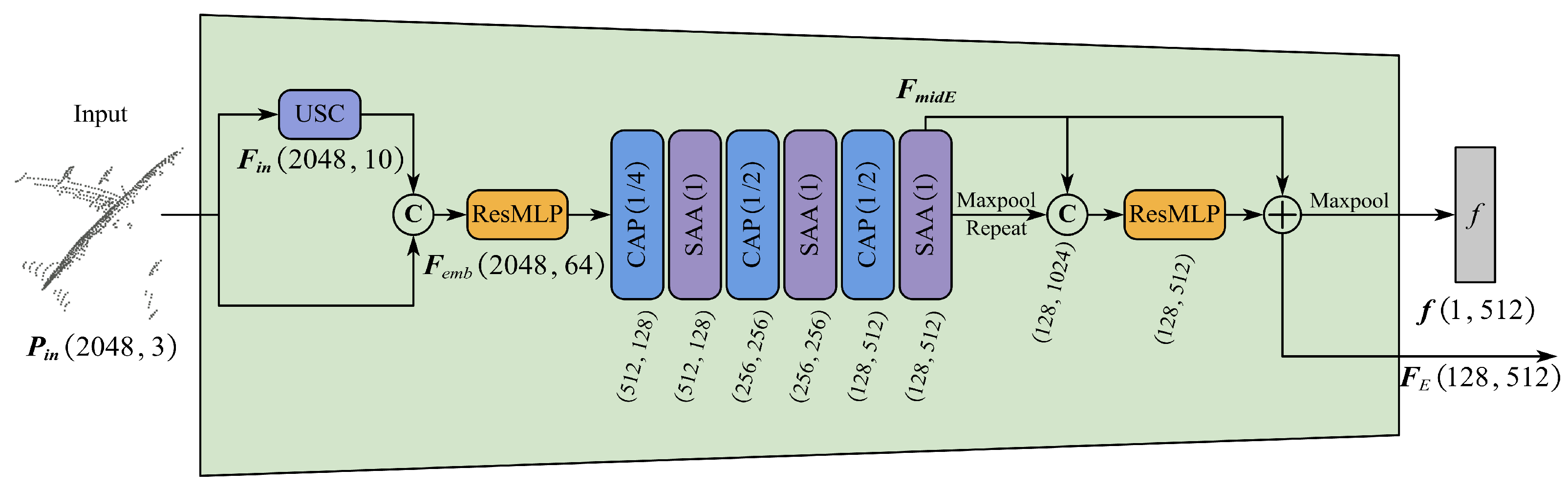
3.2. Feature Extractor

The KASiam takes the point cloud ${\mathit{P}}_{\mathit{in}}=\left\{x_i,y_i,z_i\right\}\subseteq {\mathbb{R}}^3$ of size $2048\times 3$ as its input, which contains 2048 points and only their 3D coordinate information. The feature extractor aims to generate a feature vector $\mathit{f}$ of size $1\times 512$, which can aggregate both local geometric details and global shapes by searching neighborhoods of query points adaptively. As shown in Figure 2, inspired by RepSurf [18], we feed ${\mathit{P}}_{\mathit{in}}$ into the block of umbrella surface constructor (USC). USC expands the feature dimension of ${\mathit{P}}_{\mathit{in}}$ to 10 by calculating the normal vectors, surface positions, centroid positions and polar auxiliaries of each point in ${\mathit{P}}_{\mathit{in}}$, which are beneficial for the point cloud completion task. Then, we connect it to ${\mathit{P}}_{\mathit{in}}$ again and send it to a ResMLP block to perform an operation of position embedding to obtain the embedded feature matrix ${\mathit{F}}_{\mathit{emb}}$ of size $2048\times 64$, which is formulated by Equation (1). The ResMLP blocks stand for an MLP layer with a residual structure, and are able to deepen the network to extract high-dimensional features while preventing overfitting:

$${\mathit{F}}_{\mathit{emb}}=\mathrm{ResMLP}\left(\mathrm{Concat}(\mathrm{USC}\left({\mathit{P}}_{\mathit{in}}\right),{\mathit{P}}_{\mathit{in}})\right)$$

(1)

Then, we alternately stack three CAP blocks and three SAA blocks, to increase the receptive field of points and embed both local and global geometric features during the process of down-sampling. CAPs are used to perceive the geometric details of point clouds by cross-attention operations. The down-sampling ratios of the three CAPs are 4, 2, and 2, to down-sample the point number of ${\mathit{P}}_{\mathit{in}}$ from 2048 to 128. Moreover, SAAs are used to enhance useful features for completion tasks by self-attention operations. The up-sampling ratios of the three SAAs are 1, 1, and 1. The structure details of CAP and SAA are introduced in Section 3.5. We send ${\mathit{F}}_{\mathit{emb}}$ to the above stacked CAP and SAA blocks and obtain the middle feature matrix ${\mathit{F}}_{\mathit{midE}}$ of size $128\times 512$, which is formulated as follows:

$${\mathit{F}}_{\mathit{midE}}={\left(\mathrm{SAA}\left(\mathrm{CAP}\left({\mathit{F}}_{\mathit{emb}}\right)\right)\right)}^{\left(3\right)}$$

(2)

To integrate the relationship between global features and local features, we send ${\mathit{F}}_{\mathit{midE}}$ to a layer of Max-pooling and concatenate it with ${\mathit{F}}_{\mathit{midE}}$ again. Then, we send them to a ResMLP block and form residual connection with ${\mathit{F}}_{\mathit{midE}}$, to get the encoder feature matrix ${\mathit{F}}_{\mathit{E}}$ of size $128\times 512$, which is formulated by Equation (3). Put ${\mathit{F}}_{\mathit{E}}$ into the second Max-pooling layer to get the output of the feature extractor module $\mathit{f}$ of size $1\times 512$, which is a feature vector containing shape features of the input point cloud and formulated by Equation (4). Moreover, ${\mathit{F}}_{\mathit{E}}$ acts as a carrier of shape features and transfers it to the following module.

$${\mathit{F}}_{\mathit{E}}={\mathit{F}}_{\mathit{midE}}+\mathrm{ResMLP}\left(\mathrm{Concat}(\mathrm{Maxpool}\left({\mathit{F}}_{\mathit{midE}}\right),{\mathit{F}}_{\mathit{midE}})\right)$$

(3)

$$\mathit{f}=\mathrm{Maxpool}\left({\mathit{F}}_{\mathit{E}}\right)$$

(4)

3.3. Keypoint Generator

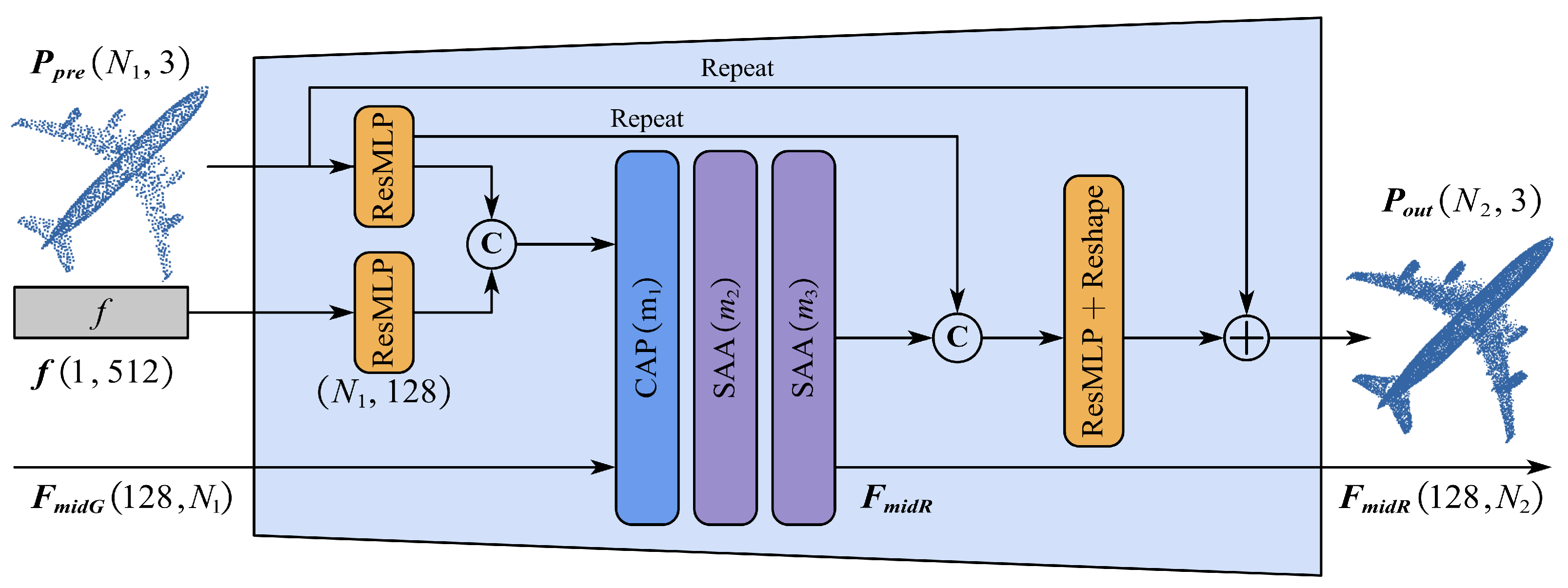
The role of the keypoint generator is to produce coarse but complete keypoints ${\mathit{P}}_{\mathit{key}}$ of inputs by decoding the feature vector $\mathit{f}$ and the shape features ${\mathit{F}}_{\mathit{E}}$, which are sent from the feature extractor. As shown in Figure 3, $\mathit{f}$ is firstly decoded into a feature matrix of size $128\times 64$ by a layer of an MLP and a convtranspose [43] operation. Convtranspose operations can expand the feature dimensions and reshape the relationship between dimensions, and are widely used in generative tasks. Then, we put the feature matrix into another layer of ResMLP to generate ${\mathit{F}}_{\mathit{ConvT}}$ of size $128\times 512$, which is formulated as follows:

$${\mathit{F}}_{\mathit{ConvT}}=\mathrm{ResMLP}\left(\mathrm{ConvT}\left(\mathrm{ResMLP}\left(\mathit{f}\right)\right)\right)$$

(5)

Then, we take ${\mathit{F}}_{\mathit{ConvT}}$ and ${\mathit{F}}_{\mathit{E}}$ as inputs to a CAP block for fusing the previous genetic shape features ${\mathit{F}}_{\mathit{E}}$ into the current shape features ${\mathit{F}}_{\mathit{ConvT}}$, which is achieved by an operation of a cross-attention mechanism. After that, we feed the output of the CAP block into two tandem SAA blocks for feature enhancements with the aid of the self-attention mechanism, and then obtain the output ${\mathit{F}}_{\mathit{midG}}$ of size $128\times 512$, which is formulated by Equation 6. The sampling ratios of the CAP and SAAs are 1, 1, 1.

$${\mathit{F}}_{\mathit{midG}}=\mathrm{SAA}\left(\mathrm{SAA}\left(\mathrm{CAP}\left({\mathit{F}}_{\mathit{ConvT}},{\mathit{F}}_{\mathit{E}}\right)\right)\right)$$

(6)

To ensure the density consistency of the generated keypoints, we send ${\mathit{F}}_{\mathit{midG}}$ to a layer of ResMLP and reshape it to a size of $512\times 3$. Since partial point clouds are also true sampling points of objects surfaces, we concatenate the above output and ${\mathit{P}}_{\mathit{in}}$, and obtain the keypoints ${\mathit{P}}_{\mathit{key}}$ of ${\mathit{P}}_{\mathit{in}}$ by a layer of FPS [16]. The size of ${\mathit{P}}_{\mathit{key}}$ is $512\times 3$, which is formulated by Equation (7). For easy understanding, we take the output of 512 keypoints as an example; other completion tasks with different numbers of points in different datasets can also be processed by setting the parameters properly. Moreover, ${\mathit{F}}_{\mathit{midG}}$ also acts as a carrier of shape features and transfers it to the following module.

$${\mathit{P}}_{\mathit{key}}=\mathrm{FPS}(\mathrm{Concat}(\mathrm{Reshape}\left(\mathrm{ResMLP}\left({\mathit{F}}_{\mathit{midG}}\right)\right),{\mathit{P}}_{\mathit{in}}),512)$$

(7)

3.4. Shape Refiner

Shape refiners aim to produce the fine-grained point cloud ${\mathit{P}}_{\mathit{out}}$ of size $N_2\times 3$ by receiving the feature vector $\mathit{f}$, the previous point cloud ${\mathit{P}}_{\mathit{pre}}$ of size $N_1\times 3$ and the shape features matrix ${\mathit{F}}_{\mathit{midG}}$ from the previous module as their inputs. As shown in Figure 4, we firstly send the previous point cloud ${\mathit{P}}_{\mathit{pre}}$ and feature vector $\mathit{f}$ to ResMLP layers separately, and then concatenate their outputs as ${\mathit{F}}_{\mathit{concat}}$ to maintain the features of local details and global shapes, which is formulated as follows:

$${\mathit{F}}_{\mathit{concat}}=\mathrm{Concat}(\mathrm{ResMLP}\left(\mathit{f}\right),\mathrm{ResMLP}\left({\mathit{P}}_{\mathit{pre}}\right))$$

(8)

Then, we take ${\mathit{F}}_{\mathit{concat}}$ and ${\mathit{F}}_{\mathit{midG}}$ as inputs to a CAP block for fusing the previous genetic shape features ${\mathit{F}}_{\mathit{midG}}$ into the current shape features ${\mathit{F}}_{\mathit{concat}}$, which is achieved by an operation of cross-attention mechanism and is similar to the operation of the keypoint generator module. After that, we send the output of the CAP block into two tandem SAA blocks for feature enhancements with the aid of a self-attention mechanism, and then get the output ${\mathit{F}}_{\mathit{midR}}$ of size $128\times N_2$, which is formulated by Equation (9). The up-sampling ratios of the CAP and SAAs are $m_1,m_2,m_3$, respectively:

$${\mathit{F}}_{\mathit{midR}}=\mathrm{SAA}\left(\mathrm{SAA}\left(\mathrm{CAP}\left({\mathit{F}}_{\mathit{concat}},{\mathit{F}}_{\mathit{midG}}\right)\right)\right)$$

(9)

The purpose of shape refiners is to generate finer shapes on coarse but complete point clouds, so it is very important and practical to estimate coordinate offsets of input point clouds. We concatenate ${\mathit{F}}_{\mathit{midR}}$ with the transformed feature matrix of the input point cloud ${\mathit{P}}_{\mathit{pre}}$, and feed them to a ResMLP layer to generate coordinate offsets. Finally, we add the coordinate offsets and the input point cloud ${\mathit{P}}_{\mathit{pre}}$ to predict a finer point cloud ${\mathit{P}}_{\mathit{out}}$, which is formulated by Equation (10). Moreover, ${\mathit{F}}_{\mathit{midR}}$ also acts as a carrier of shape features and transfers it to the following module, until this shape refiner is the last one and the resolution of the generated point cloud meets the requirements.

$${\mathit{P}}_{\mathit{out}}={\mathit{P}}_{\mathit{pre}}+\mathrm{Reshape}\left(\mathrm{ResMLP}\left(\mathrm{Concat}(\mathrm{ResMLP}\left({\mathit{P}}_{\mathit{pre}}\right),{\mathit{F}}_{\mathit{midR}})\right)\right)$$

(10)

3.5. Cross-Attention Perception and Self-Attention Augment

In this section, we focus on structures of cross-attention perception and self-attention augment blocks. It is important for point cloud completion to capture suitable geometric features. Existing local shape extraction methods with kNNs are easily affected by the local density of the point cloud and outliners, so we abandon the KNN operation and replace it with pure attention mechanisms. As shown in Figure 5, they have similar structures, especially the core layer of multi-head attention mechanisms.

3.5.1. Cross-Attention Perception Block

The structure of CAP is illustrated in the top of Figure 5. Each CAP has two feature matrices as inputs, which are the current feature matrix ${\mathit{F}}_{\mathit{cur}}$ and the shape feature matrix ${\mathit{F}}_{\mathit{pre}}$ from the previous module. It is worth noting that the feature extractor is the first module in the network, so we regard the down-sampling of ${\mathit{F}}_{\mathit{cur}}$ as ${\mathit{F}}_{\mathit{pre}}$ in three CAP blocks in the feature extractor. We generate the Value and Key matrices from ${\mathit{F}}_{\mathit{cur}}$ and generate the Query matrix from ${\mathit{F}}_{\mathit{pre}}$ by different MLP layers respectively. Then, we adopt a layer of the multi-head cross-attention in the form of residual with Query to learn a new feature matrix ${\mathit{F}}_{\mathit{mid}}$, which is formulated as follows:

$$\mathit{Q}=\mathrm{MLP}\left({\mathit{F}}_{\mathit{pre}}\right),\mathit{K}=\mathrm{MLP}\left({\mathit{F}}_{\mathit{cur}}\right),\mathit{V}=\mathrm{MLP}\left({\mathit{F}}_{\mathit{cur}}\right)$$

(11)

$${\mathit{F}}_{\mathit{mid}}=\mathrm{BN}(\mathit{Q}+\mathrm{MultiHead}(\mathit{Q},\mathit{K},\mathit{V}))$$

(12)

Here, $\mathrm{MultiHead}$ is performed similarly to Transformer [11]. After the attention operation, each point in ${\mathit{F}}_{\mathit{pre}}$ can adaptively aggregate noteworthy features from ${\mathit{F}}_{\mathit{cur}}$ to perceive the local geometric structure of point clouds.

Then, to enhance the representation ability of CAP, we send ${\mathit{F}}_{\mathit{mid}}$ to an MLP layer with an inverted residual bottleneck design, to update ${\mathit{F}}_{\mathit{mid}}$ and enhance the representation ability of CAP. Finally, if in the feature extractor, we concatenate the updated feature matrix with ${\mathit{F}}_{\mathit{pre}}$ to generate the output of the CAP block as follows:

$${\mathit{F}}_{\mathit{out}}=\mathrm{Concat}({\mathit{F}}_{\mathit{pre}},{\mathit{F}}_{\mathit{mid}}+\mathrm{MLP}\left({\mathit{F}}_{\mathit{mid}}\right))$$

(13)

3.5.2. Self-attention Augment Block

The structure of SAA is illustrated at the bottom of Figure 5, which is similar to CAP and has an additional channel attention block. The role of SAA is to establish the spatial relationship among points and enhance the feature representation ability of the network. Each SAA takes the current feature matrix ${\mathit{F}}_{\mathit{cur}}$ as the only input. We generate the Query, Key and Value matrices from ${\mathit{F}}_{\mathit{cur}}$ by different MLP layers respectively. Then, we adopt a layer of the multi-head self-attention in the form of residual with Query to learn a new feature matrix ${\mathit{F}}_{\mathit{mid}}$, which is formulated as follows:

$$\mathit{Q}=\mathrm{MLP}\left({\mathit{F}}_{\mathit{cur}}\right),\mathit{K}=\mathrm{MLP}\left({\mathit{F}}_{\mathit{cur}}\right),\mathit{V}=\mathrm{MLP}\left({\mathit{F}}_{\mathit{cur}}\right)$$

(14)

$${\mathit{F}}_{\mathit{mid}}=\mathrm{BN}(\mathit{Q}+\mathrm{MultiHead}(\mathit{Q},\mathit{K},\mathit{V}))$$

(15)

After that, similar to CAP, we send ${\mathit{F}}_{\mathit{mid}}$ to an MLP layer with an inverted residual bottleneck design, to update ${\mathit{F}}_{\mathit{mid}}$ and enhance the representation ability of SAA. Then, we concatenate the updated feature matrix with ${\mathit{F}}_{\mathit{cur}}$ to generate the input feature matrix of the channel attention block ${\mathit{F}}_{\mathit{inCA}}$ as follows:

$${\mathit{F}}_{\mathit{inCA}}=\mathrm{Concat}({\mathit{F}}_{\mathit{cur}},{\mathit{F}}_{\mathit{mid}}+\mathrm{MLP}\left({\mathit{F}}_{\mathit{mid}}\right))$$

(16)

Inspired by the squeeze-and-excitation networks (SENet [44]) in image processing, we propose a channel attention block to SAA, to augment useful features of geometric details for the completion of point clouds. As shown in Figure 6, the channel attention block adopts a similar squeeze-and-excitation structure on 3D point clouds. We firstly squeeze the input feature matrix ${\mathit{F}}_{\mathit{inCA}}$ of size $N\times C$ into a channel descriptor, which is achieved by using a global average pooling operation to generate channel-wise statistics. Then, we feed the descriptor to an FC layer with a bottleneck structure, to learn the attention weight of each channel. Finally, we can get a weighted feature matrix ${\mathit{F}}_{\mathit{out}}$ by a dot product operation between ${\mathit{F}}_{\mathit{inCA}}$ and the channel attention weight, which is formulated as follows:

$${\mathit{F}}_{\mathit{out}}=\mathrm{Channel-Attention}\left({\mathit{F}}_{\mathit{inCA}}\right)={\mathit{F}}_{\mathit{inCA}}\odot \mathrm{FC}(\sum _{i=1}^N{\mathit{F}}_{\mathit{inCA}}(i,j)/N)$$

(17)

3.6. Training Loss

As mentioned in the Section 3.1, KASiam has dual input-asymmetric paths, which are the reconstruction path and the completion path, respectively. The training losses of the two paths are different. We use the loss functions of the Chamfer distance (CD), the Earth Mover’s Distance (EMD) and the Root Mean Square Error (RMSE) for the calculation of training losses, which are formulated as follows:

$$d_{CD}(\mathcal{P},\mathcal{Q})=\frac{1}{\left|\mathcal{P}\right|}\sum _{p\in \mathcal{P}}\underset{q\in \mathcal{Q}}{min}\parallel p-q\parallel +\frac{1}{\left|\mathcal{Q}\right|}\sum _{q\in \mathcal{Q}}\underset{p\in \mathcal{P}}{min}\parallel q-p\parallel$$

(18)

$$d_{EMD}(\mathcal{P},\mathcal{Q})=\underset{\varphi :\mathcal{P}\to \mathcal{Q}}{min}\frac{1}{\left|\mathcal{P}\right|}\sum _{x\in \mathcal{P}}{\parallel x-\varphi \left(x\right)\parallel }_2$$

(19)

$$d_{RMSE}(\mathit{f},\mathit{h})=\sqrt{\frac{1}{n}\sum _n{(\mathit{f}-\mathit{h})}^2}$$

(20)

where $\mathcal{P}$ and $\mathcal{Q}$ are two point clouds with the same number of points and $\mathit{f}$ and $\mathit{h}$ are two feature vectors with the same length. CD represents the average distance of the closest point between two point clouds. EMD aims to find out a bijection to minimize the average distance between corresponding points from partial and complete ones. RMSE explicitly measures the difference between two vectors.

3.6.1. Loss in the Reconstruction Path

In the reconstruction path, we use the combination of CD and EMD as a difference measure of point clouds to formulate the training loss of reconstruction. We down-sample the ground truth point cloud to {${\mathit{GT}}_{\mathit{key}},{\mathit{GT}}_{\mathit{mid}},{\mathit{GT}}_{\mathit{fine}}$}, which has the same point number as {${\widehat{\mathit{P}}}_{\mathit{key}},{\widehat{\mathit{P}}}_{\mathit{mid}},{\widehat{\mathit{P}}}_{\mathit{fine}}$}, and the loss is as follows:

$${\mathcal{L}}_{reconstruction}=d_{\mathrm{CD}}({\widehat{\mathit{P}}}_{\mathit{key}},{\mathit{GT}}_{\mathit{key}})+d_{\mathrm{EMD}}({\widehat{\mathit{P}}}_{\mathit{mid}},{\mathit{GT}}_{\mathit{mid}})+d_{\mathrm{CD}}({\widehat{\mathit{P}}}_{\mathit{fine}},{\mathit{GT}}_{\mathit{fine}})$$

(21)

It is worth noting that we use EMD to calculate the loss of ${\widehat{\mathit{P}}}_{\mathit{mid}}$ and ${\mathit{GT}}_{\mathit{mid}}$, which are point clouds with medium resolution in the whole pipeline of reconstruction, becaue we find that this operation can give consideration to both performance and efficiency by experiments.

3.6.2. Loss in Completion Path

In the completion path, we use the combination of RMSE, CD and EMD as a difference measure of point clouds to formulate the training loss of completion. The total loss is as follows:

$${\mathcal{L}}_{completion}={\alpha }_1\times [d_{RMSE}(\mathit{f},\widehat{\mathit{f}})+d_{\mathrm{CD}}({\mathit{P}}_{\mathit{key}},{\widehat{\mathit{P}}}_{\mathit{key}})]+{\alpha }_2\times d_{\mathrm{EMD}}({\mathit{P}}_{\mathit{mid}},{\mathit{GT}}_{\mathit{mid}})+{\alpha }_3\times d_{\mathrm{CD}}({\mathit{P}}_{\mathit{fine}},{\mathit{GT}}_{\mathit{fine}})$$

(22)

where ${\alpha }_1$, ${\alpha }_2$ and ${\alpha }_3$ are changeable hyperparameters during the training stage of the completion path. To make full use of geometric features of complete shapes and improve the quality of the generated point clouds, we apply keypoints alignment operations by minimizing the loss functions $d_{RMSE}(\mathit{f},\widehat{\mathit{f}})$ and $d_{\mathrm{CD}}({\mathit{P}}_{\mathit{key}},{\widehat{\mathit{P}}}_{\mathit{key}})$.

4. Experiments and Results

4.1. Datasets and Implementation Details

The proposed KASiam is evaluated on the standard PCN [5] benchmark, which is derived from the ShapeNet [45] dataset, and some TLS data scanned by a RigelScan LiDAR. PCN is a widely used benchmark of point cloud completion, which contains 30,974 complete-partial point cloud pairs of eight categories. The partial point clouds are generated by back-projecting complete 3D shapes into eight different views. For each ground-truth point cloud, 16,384 points are evenly sampled from the shape surface. For a fair comparison, we follow the same train/val/test split settings as PCN [5], 28,974 pairs for training, 800 pairs for validation and 1200 pairs for testing. Only the 28,974 training pairs are trained by our network, the unseen 800 validation pairs and 1200 testing pairs are tested directly for adjusting parameters of the network and comparisons with other methods, respectively. Moreover, we adopt the L1 version of Chamfer distance to evaluate the models.

To verify the effectiveness of KASiam on LiDAR point clouds, we scan several objects partially and completely with a RigelScan LiDAR; most objects are selected from our laboratory, only planes and sport cars are high-fidelity models. The parameters of the LiDAR are listed in the

Table 1. Main parameters of the RigelScan LiDAR.

RigelScan	Repetition Rate	Scanning Beam	Range Resolution
Standard mode	205,000 fps	14	0.05 mm
Fine mode	320,000 fps	14	0.03 mm

. We scan the objects from a single viewpoint and completely to obtain the original partial and complete point clouds, respectively. To match the parameters of the model, we manually remove the background points in the original data and down-sample the partial and the complete point clouds to 2048 and 16,384 points as our inputs and ground truths, respectively. It is worth noting that we load the pretrained PCN model and use the TLS data only for testing.

All the experiments are trained on a graphics workstation, which is installed with AMD Ryzen 7 5800X CPU (3.8 GHz, 8 cores), 32 GB RAM and two NVIDIA GTX 3090 GPUs. We adopt the framework of Pytorch 1.10 with Python 3.8 and CUDA 11.3. We train the model with Adam optimizer for a total of 400 epochs, while the learning rate is initialized to 1 × 10${}^{-4}$ and decayed by 0.7 every 50 epochs. The batch size is set to 32, and the hyperparameters in the training loss of the completion path are set as the

Table 2. The setting of hyperparameters in the training loss of the completion path.

Epoch	${\mathit{\alpha }}_1$	${\mathit{\alpha }}_2$	${\mathit{\alpha }}_3$
1–50	1	0	0
50–75	0	1	0.1
75–100	0	1	0.5
100–200	0	1	1
200–400	0	0	1

. For experiments on the PCN dataset and our TLS data, we set the up-sampling ratios $m_1,m_2,m_3$ in the two shape refiners as (1, 1, 4) and (1, 1, 8), respectively.

4.2. Results on the PCN Dataset

Table 3. Point cloud completion quantitative results on the PCN dataset in terms of L1 Chamfer distance ($\times {10}^{-3}$). The best results are highlighted in boldface.

Methods	Average	Plane	Cabinet	Car	Chair	Lamp	Couch	Table	Boat
FoldingNet [32]	14.31	9.49	15.80	12.61	15.55	16.41	15.97	13.65	14.99
TopNet [7]	12.15	7.61	13.31	10.90	13.82	14.44	14.78	11.22	11.12
AtlasNet [46]	10.85	6.37	11.94	10.10	12.06	12.37	12.99	10.33	10.61
PCN [5]	9.64	5.50	22.70	10.63	8.70	11.00	11.34	11.68	8.59
GRNet [3]	8.83	6.45	10.37	9.45	9.41	7.96	10.51	8.44	8.04
PMP-Net [35]	8.73	5.65	11.24	9.64	9.51	6.95	10.83	8.72	7.25
CRN [9]	8.51	4.79	9.97	8.31	9.49	8.94	10.69	7.81	8.05
PoinTr [12]	8.38	4.75	10.47	8.68	9.39	7.75	10.93	7.78	7.29
NSFA [8]	8.06	4.76	10.18	8.63	8.53	7.03	10.53	7.35	7.48
SnowflakeNet [10]	7.21	4.29	9.16	8.08	7.89	6.07	9.23	6.55	6.40
KASiam (Ours)	6.87	3.90	9.28	8.02	7.21	5.51	8.82	6.25	5.96

enumerates the quantitative results of KASiam and other completion methods on the PCN dataset; KASiam achieves the best performance in almost all categories, and significantly reduces the average CD by 0.34 (4.72%) as compared with SnowflakeNet [10] and 2.77 (28.73%) as compared with PCN [5], which proves that our method is able to complete finer point clouds. Specifically, in the categories of plane, chair and lamp, our method reduces the CD more than 8% as compared with SnowflakeNet [10], and the CD of lamps reduces the most (9.2%). It is also worth noting that there is little reduction in the category of car and even a little rise in the category of cabinet. Because objects within these two categories are of similar shapes, this limits the advantage of KASiam in dealing with various shapes. In particular, the objects of cabinet have a large number of points with internal shapes, which is not conducive to the completion of point cloud surfaces.

We choose PCN [5], SnowflakeNet [10] and KASiam point clouds completion methods from Table 3, and visually compare the completion results of them in eight categories in Figure 7. We can observe that the shapes generated by our method have smoother surfaces, more detailed shapes and more semantic structures. Specifically, we summarize the advantages of our method into three types.

Firstly, KASiam can produce complete and smooth surfaces without outliers. For example, as for the cabinet, KASiam is able to keep the inside structure hollow during the process of completion, while PCN and SnowflakeNet fill the hollow structure with lots of noise points, which do not conform to the true shape of the cabinet. As for the lamp, KASiam is able to generate the complete lampshade and the straight lamppost. However, there are some outliers around the lampshade generated by SnowflakeNet, and it is difficult for PCN to identify and complete the lampshade structure. A similar event occurs during the completion of the boat: the mast generated by KASiam is the straightest and has few outliers.

Secondly, KASiam can capture and generate more realistic and semantic object structures. For example, as for the chair, KASiam can capture and augment the feature of the top region, and accurately generate the back of the chair with two tips, while PCN and SnowflakeNet fail to capture the structure of two tips and generate an ordinary flat top of the chair back. As for the table, PCN and SnowflakeNet ignore the shape of the tablecloth on the desktop, and generate lots of messy points in the area. However, KASiam can accurately capture the triangular structure of the tablecloth and complete it. As for the couch, the difficulty lies in the completion process of the pillow on the couch. KASiam identifies the existence of the pillow accurately, and generates the complete pillow according to the existing shapes. However, PCN and SnowflakeNet only pay attention to the completion of the overall shape of the couch, and ignore the detailed structure of the other objects.

Thirdly, KASiam is good at extracting features from existing parts of objects and generating whole ones with detailed shapes. For example, as for the plane, KASiam can generate the precise shapes of the missing engine and tyre of the plane, by aggregating the shape features of existing structures on the other side. However, the wing generated by SnowflakeNet does not have the same density as the wing on the other side, and PCN neglects the completion of the tyre of the plane. As for the car, the difficulty lies in the process of completion of the slanting tyres under the car. KASiam can generate the slanting tyre by referencing the orientation of the existing tyre on the other side. However, SnowflakeNet generates a normal tyre just like the shapes of most of ordinary tyres in cars in the training dataset, and PCN ignores the completion of the slanting tyre and the rearview mirror.

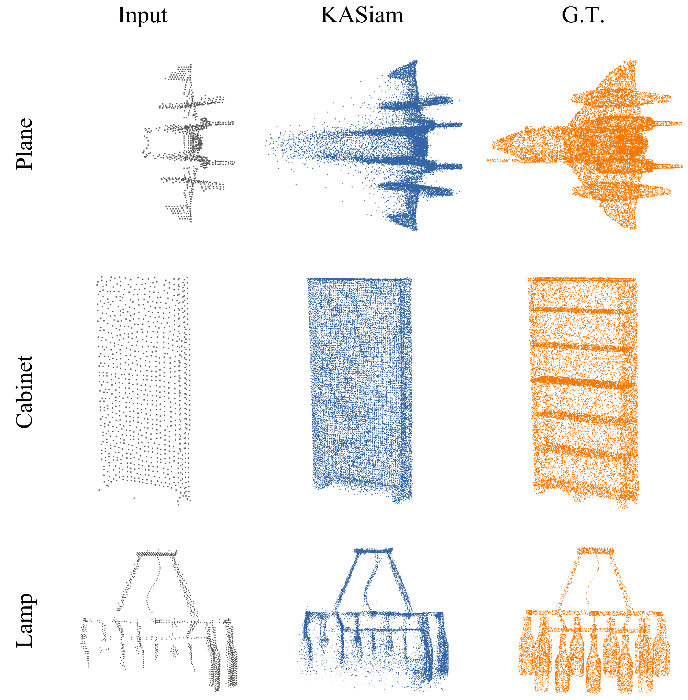
4.3. Results on the TLS Data

To verify the effectiveness of KASiam on LiDAR point clouds, we scan several objects partially and completely with a RigelScan LiDAR (Table 1 for more details). To match the parameters of our pre-trained model, we down-sample the partial and the complete scans to 2048 and 16,384 points, respectively, to serve as the inputs and ground truths of our model.

We choose the top 2 point clouds completion methods SnowflakeNet [10] and KASiam from Table 3, and visually compare the TLS completion results of them in three common categories in Figure 8. Our method, KASiam, can mitigate the impact of the data density distribution and generate more accurate shapes, which is crucial to the field of remote sensing and TLS analysis.

As shown in Figure 8, KASiam can generate the missing leg of the chair by capturing and extracting shape features of the remaining three legs, and makes a basic completion of the ring structure at the bottom of the chair. However, SnowflakeNet generates a bad shape of the missing leg with lots of noise points and different densities from existing ones. As for the plane, KASiam can complete the protruding auxiliary wing perfectly, which is failed in SnowflakeNet. As for the car, KASiam is able to capture and generate the window structure of the sport car accurately. However, the window structure generated by SnowflakeNet is filled with lots of noise points.

4.4. Ablation Studies and Analyses

In order to examine the effectiveness of each module of our method, we stack the proposed blocks on the baseline step-to-step to form five variations ($\mathcal{A}-\mathcal{E}$) in

Table 4. Ablation study of KASiam on the PCN dataset in terms of L1 Chamfer distance ($\times {10}^{-3}$). Here, USC, CAP, SAA and CA represent the blocks of umbrella surface constructor [18], cross-attention perception, self-attention augment and channel attention, respectively. The best results are highlighted in boldface.

	USC	CAP	SAA	CA	Shape Refiner	Average	Plane	Chair	Lamp	Boat
$\mathcal{A}$		✓	✓	✓	✓	6.92	3.92	7.32	5.59	6.02
$\mathcal{B}$	✓		✓	✓	✓	7.25	4.53	8.43	6.40	6.99
$\mathcal{C}$	✓	✓		✓	✓	7.08	4.42	8.17	6.23	6.65
$\mathcal{D}$	✓	✓	✓		✓	7.01	4.27	8.02	6.12	6.34
$\mathcal{E}$	✓	✓	✓	✓		8.35	5.31	9.74	7.34	7.94
Full	✓	✓	✓	✓	✓	6.87	3.90	7.21	5.51	5.96

. By default, except for examined blocks, all structures of variations and the experiment settings remain the same. We train these models on the whole PCN dataset and only show four highly different categories (plane, chair, lamp and table) in the table. Five different network variations are designed as follows:

• Variation $\mathcal{A}$. To examine the effectiveness of USC block for point cloud generations, we remove the USC block and send the input point cloud to the layer of position embedding directly.
• Variation $\mathcal{B}$. To examine the effectiveness of CAP blocks in the feature extractor module, we replace all the CAP blocks in the feature extractor with layers of PointNet++ [16].
• Variation $\mathcal{C}$. To examine the effectiveness of SAA blocks in the feature extractor module, we remove all the SAA blocks in the feature extractor and connect the stacked CAPs directly.
• Variation $\mathcal{D}$. To examine the effectiveness of CA blocks in the feature extractor module, we remove all the CA blocks in the SAA blocks, while the other structures of the network remain unchanged.
• Variation $\mathcal{E}$. To examine the effectiveness of the shape refiner modules for point cloud generations, we replace all shape refiner modules with the generation operation based on FoldingNet [32].

As shown in Table 4, the full KASiam model achieves the best performance. Specifically, comparing with Variation $\mathcal{A}$, the USC block can bring a little gain to the network performance, which is likely that the parameters explicitly calculated by USC are beneficial for the point cloud completion task. Comparing with Variation $\mathcal{B}$, the average CD can be 5.2% lower by applying CAPs to the feature extractor, which demonstrates that the CAP blocks can select neighborhoods of query points adaptively to capture and extract shape features of partial point clouds. Comparing with Variation $\mathcal{C}$, the average CD is reduced by 0.21 and SAA blocks in the feature extractor are crucial for deep feature extraction. The comparison between $\mathcal{D}$ and the default KASiam demonstrates that the channel attention blocks in the SAA blocks are helpful in augmenting useful features of geometric shapes selectively. Comparing with Variation $\mathcal{E}$, the average CD can be 17.7% lower by applying shape refiner modules, which have the ability to generate point clouds with more detailed structures and smoother surfaces than the manifold fitting method [32].

4.4.1. Visualization Analysis of Attention Mechanisms on Point Clouds

In this section, we make extensive visualization analyses of the attention mechanisms on point clouds to show the effectiveness of CAP and SAA blocks visually. As shown in Figure 9, these analyses can be divided into three aspects: different methods of neighborhood selection, different attention layers and different positions of query points.

As shown in Figure 9a, we compare different neighborhood selection methods of query points between the traditional KNN, Global-KNN [15] and our KASiam, we set the number of neighbors in KNN to 64 and select the results of the first CAA layer as outputs of KASiam. KNN only selects neighborhoods closest to the query point according to the Euclidean distance. Global-KNN [15] improves the KNN operation and can select neighborhoods of the query point according to semantic features, but the number of neighbors is as limited as KNN. However, our KASiam has the ability to search neighborhoods of query points adaptively by multi-head attention operations, to capture and aggregate shape features of all points according to semantic shape features.

As shown in Figure 9b, we compare the outputs of different CAA layers in the feature extractor. Visualization results demonstrate that, with the deepening of the layers, our KASiam can select neighborhoods in shape regions similar to the query point at the semantic level, rather than simply according to the Euclidean distance. For example, the query point close to the aircraft fuselage gradually transfers the attentive region from the wing to the fuselage through the network fitting of CAA blocks. A similar event occurs on the chair; the query point at the beam of the chair should pay more attention to the beams and legs of the chair rather than the chair back.

As shown in Figure 9c, we explore the relationship between attentive regions and positions of query points. We select results of the second CAA layer as outputs to make the comparison more obvious. Visualization results demonstrate that our KASiam can capture attentive regions adaptively according to different semantic shapes of query points. For example, if the query point is on the tyre area, the attentive region of it should be close to the area of similar structures of tyres. If the query point is on the car hood, the attentive region of it should be the front region of the car. Moreover, we provide more results of attention mechanisms on other objects in Figure 9d.

4.4.2. Visualization Analysis of the Keypoints Alignment Operation

In this section, we make some visualization analyses of the keypoints alignment operation during point cloud completion in Figure 10. After training in the reconstruction path, we get the accurate keypoints distribution with complete point clouds as inputs. Then, we constantly calculate the Chamfer Distance $d_{\mathrm{CD}}({\mathit{P}}_{\mathit{key}},{\widehat{\mathit{P}}}_{\mathit{key}})$ between keypoints generated by the completion path and the reconstruction path (Section 3.6.2), and let it act as a part of the loss function ${\mathcal{L}}_{completion}$ in the completion path. The role of the Keypoints Alignment Operation is to make the distribution of completion path keypoints ${\mathit{P}}_{\mathit{key}}$ close to reconstruction path ones ${\widehat{\mathit{P}}}_{\mathit{key}}$, which is beneficial to generate fine-grained point clouds with highly detailed geometric shapes.

Take the completion of a partial plane as an example. In epoch 2, there are few keypoints located in the area of the missing wing and engine, which is detrimental to generating a complete aircraft shape. With the training of the completion path, we find that keypoints are distributed almost throughout the region of the missing wing and engine in epoch 200. It is an important and fundamental step for generating a complete point cloud of the plane. Moreover, we provide more results of the keypoints alignment operation on more objects in Figure 10b. The results show that the keypoints generated by KASiam are distributed on the surface of the corresponding object evenly, and demonstrate that the keypoints alignment operation has the ability to capture and recover the geometry of objects, and is beneficial to point cloud completion tasks.

4.4.3. Visualization analysis of the Shape Refiners

In this section, we make some visualization results of the process of point clouds completion by shape refiners in Figure 11. As mentioned in Section 3.4, the purpose of shape refiners is to generate finer point clouds from a coarse one and transfer shape feature information. Specifically, each shape refiner first duplicates the former point cloud ${\mathit{P}}_{\mathit{pre}}$ and then adds variations to generate the current point cloud ${\mathit{P}}_{\mathit{out}}$, which can be estimated by the aid of CAP and SAA blocks. As shown in Figure 11, we enumerate the generation process of point clouds for eight objects. Shape refiners have the ability to refine the point cloud step by step (${\mathit{P}}_{\mathit{key}}\to {\mathit{P}}_{\mathit{mid}}\to {\mathit{P}}_{\mathit{fine}}$) based on the accurate keypoints. Even if the keypoints have inaccurate or missing areas, shape refiners can also identify and correct them accurately. The results demonstrate that shape refiners are able to interpret the shape features of former objects accurately and generate point clouds with fine-grained geometric shapes, which is instrumental in the generation of point clouds.

5. Discussion

Although the above analyses demonstrate that our KASiam has achieved great results in point cloud completion, we identify three faulty modes for our method in the PCN dataset in Figure 12.

Firstly, KASiam cannot handle rare shapes well. Taking the plane as an example, compared with other common planes, this plane has a rare shape with a nose antenna and complex wings, and has a small sample in the whole PCN dataset. Thus, KASiam has limited ability to capture and reconstruct these rare shapes due to the training strategy, which is also a common problem of supervised deep learning algorithms. Secondly, KASiam cannot reconstruct some parts of objects without any prior information in partial point clouds. Take the cabinet as an example, the input partial point cloud is scanned by a lidar placed behind the cabinet, and there are no points belonging to the hierarchical structure of the cabinet. Thus, KASiam generates an ordinary cabinet without the hierarchical structure. On the other hand, this cannot be defined as a failure case, because it is also a complete and semantic shape of cabinets under different evaluation criteria. Thirdly, KASiam cannot handle objects with numerous and detached parts. Taking the lamp as an example, KASiam mishandles the completion of the lamp with lots of detached bulbs. This is likely due to that such structures have high-frequency feature information, which is difficult to extract by neural networks.

In the future, to further solve the above problems, we think there are three directions to explore. Firstly, because most of the scanned point clouds are incomplete and unmarked, it is a trend to accomplish point cloud feature learning and point cloud completion by unsupervised learning, which can reduce the inductive bias of algorithms for specific datasets and improve categories generalization and robustness. Secondly, it is necessary to propose a new point cloud completion evaluation standard based on the semantic level, because it does not need to calculate the distance between each point in some completion tasks. Thirdly, deep graph convolution networks, or other networks that implicitly define geometric relationships between features, may be the key to further improve the feature representation ability of neural networks.

6. Conclusions

In this paper, we propose a keypoints-aligned siamese network named KASiam for the completion of partial point clouds. KASiam has dual input-asymmetric paths of reconstruction and completion with cross-attention perception (CAA) blocks and self-attention augment (SAA) blocks inserted. KASiam takes sufficient advantage of input point clouds through the keypoints alignment operation, and searches neighborhoods of query points adaptively by multi-head attention operations to capture and aggregate shape features. Experimental results and analyses on the PCN dataset and several TLS data demonstrate that KASiam achieves the state-of-the-art point cloud completion performance and can predict fine-grained shapes with highly detailed geometries in the majority of cases, which is crucial for the area of remote sensing and some TLS applications. It is worth noting that KASiam works on down-sampled TLS point clouds rather than the original TLS data for efficiency.

References

1. Guo, Y.; Wang, H.; Hu, Q.; Liu, H.; Liu, L.; Bennamoun, M. Deep Learning for 3D Point Clouds: A Survey. IEEE Trans. Pattern Anal. Mach. Intell. 2021, 43, 4338–4364. [Google Scholar] [CrossRef] [PubMed]
2. Angela, D.; Charles, R.Q.; Matthias, N. Shape Completion Using 3D-Encoder-Predictor CNNs and Shape Synthesis. In Proceedings of the IEEE Conference on Computer Vision and Pattern Recognition, Honolulu, HI, USA, 21–26 July 2017; pp. 6545–6554. [Google Scholar]
3. Xie, H.; Yao, H.; Zhou, S.; Mao, J.; Sun, W. GRNet: Gridding Residual Network for Dense Point Cloud Completion. In Proceedings of the European Conference on Computer Vision, Glasgow, Scotland, 23–28 August 2020; pp. 365–381. [Google Scholar]
4. Wang, X.; Marcelo, H.; Gim, H.L. Voxel-based Network for Shape Completion by Leveraging Edge Generation. In Proceedings of the IEEE/CVF International Conference on Computer Vision, Montreal, Canada, 11–17 October 2021; pp. 13169–13178. [Google Scholar]
5. Wang, Y.; Tejas, K.; David, H.; Christoph, M.; Martial, H. PCN: Point Completion Network. In Proceedings of the International Conference on 3D Vision, Verona, Italy, 5–8 September 2018; pp. 728–737. [Google Scholar]
6. Charles, R.Q.; Su, H.; Mo, K.; Guibas, L.J. PointNet: Deep Learning on Point Sets for 3D Classification and Segmentation. In Proceedings of the IEEE Conference on Computer Vision and Pattern Recognition, Honolulu, HI, USA, 21–26 July 2017; pp. 77–85. [Google Scholar]
7. Tchapmi, L.P.; Kosaraju, V.; Reid, I.; Savarese, S. TopNet: Structural Point Cloud Decoder. In Proceedings of the IEEE Conference on Computer Vision and Pattern Recognition, Long Beach, USA, 15–21 June 2019; pp. 383–392. [Google Scholar]
8. Zhang, W.; Yan, Q.; Xiao, C. Detail Preserved Point Cloud Completion via Separated Feature Aggregation. In Proceedings of the European Conference on Computer Vision, Glasgow, Scotland, 23–28 August 2020; pp. 512–528. [Google Scholar]
9. Wang, X.; Marcelo, H.; Gim, H.L. Cascaded Refinement Network for Point Cloud Completion. In Proceedings of the IEEE/CVF International Conference on Computer Vision, Seattle, WA, USA, 14–19 June 2020; pp. 787–796. [Google Scholar]
10. Xiang, P.; Wen, X.; Liu, Y.; Cao, Y.; Wan, P.; Zheng, W.; Han, Z. SnowflakeNet: Point Cloud Completion by Snowflake Point Deconvolution with Skip-Transformer. In Proceedings of the IEEE/CVF International Conference on Computer Vision, Montreal, QC, Canada, 11–17 October 2021; pp. 5479–5489. [Google Scholar]
11. Vaswani, A.; Shazeer, N.; Parmar, N.; Uszkoreit, J.; Jones, L.; Gomez, A.N.; Kaiser, L.; Polosukhin, I. Attention is all you need. In Proceedings of the International Conference on Neural Information Processing Systems, Long Beach, CA, USA, 4–9 December 2017; pp. 6000–6010. [Google Scholar]
12. Yu, X.; Rao, Y.; Wang, Z.; Liu, Z.; Lu, J.; Zhou, J. PoinTr: Diverse Point Cloud Completion with Geometry-Aware Transformers. In Proceedings of the IEEE/CVF International Conference on Computer Vision, Montreal, Canada, 11–17 October 2021; pp. 12478–12487. [Google Scholar]
13. Xia, Y.; Xia, Y.; Li, W.; Song, R.; Cao, K.; Stilla, U. ASFM-Net: Asymmetrical Siamese Feature Matching Network for Point Completion. In Proceedings of the ACM Multimedia Conference, Chengdu, China, 20–24 October 2021; pp. 1938–1947. [Google Scholar]
14. Pan, L.; Chen, X.; Cai, Z.; Zhang, J.; Zhao, H.; Liu, Z. Variational Relational Point Completion Network. In Proceedings of the IEEE Conference on Computer Vision and Pattern Recognition, Online, 19–25 June 2021; pp. 8520–8529. [Google Scholar]
15. Liu, X.; Xu, G.; Xu, K.; Wan, J.; Ma, Y. Point cloud completion by dynamic transformer with adaptive neighbourhood feature fusion. IET Comput. Vis. 2022, 1, 1–13. [Google Scholar] [CrossRef]
16. Charles, R.Q.; Li, Y.; Su, H.; Guibas, L.J. PointNet++: Deep hierarchical feature learning on point sets in a metric space. In Proceedings of the International Conference on Neural Information Processing Systems, Long Beach, CA, USA, 4–9 December 2017; pp. 5105–5114. [Google Scholar]
17. Ma, X.; Qin, C.; You, H.; Ran, H.; Fu, Y. Rethinking Network Design and Local Geometry in Point Cloud: A Simple Residual MLP Framework. In Proceedings of the International Conference on Learning Representations, Online, 25–29 April 2022. [Google Scholar]
18. Ran, H.; Liu, J.; Wang, C. Surface Representation for Point Clouds. arXiv 2022, arXiv:2205.05740. [Google Scholar]
19. Li, Y.; Bu, R.; Sun, M.; Wu, W.; Di, X.; Chen, B. PointCNN: Convolution On X-Transformed Points. arXiv 2018, arXiv:1801.07791. [Google Scholar]
20. Wu, W.; Qi, Z.; Li, F. PointConv: Deep Convolutional Networks on 3D Point Clouds. In Proceedings of the IEEE Conference on Computer Vision and Pattern Recognition, Long Beach, CA, USA, 15–21 June 2019; pp. 9613–9622. [Google Scholar]
21. Xu, M.; Ding, R.; Zhao, H.; Qi, X. PAConv: Position Adaptive Convolution with Dynamic Kernel Assembling on Point Clouds. In Proceedings of the IEEE Conference on Computer Vision and Pattern Recognition, Online, 19–25 June 2021; pp. 3172–3181. [Google Scholar]
22. Wang, W.; Zhou, H.; Chen, G.; Wang, X. Fusion of a Static and Dynamic Convolutional Neural Network for Multiview 3D Point Cloud Classification. Remote Sens. 2022, 14, 1996. [Google Scholar] [CrossRef]
23. Wang, Y.; Sun, Y.; Liu, Z.; Sarma, S.E.; Bronstein, M.; Solomon, J.M. Dynamic Graph CNN for Learning on Point Clouds. ACM Trans. Graph. 2018, 5, 1–12. [Google Scholar] [CrossRef] [Green Version]
24. Zhou, H.; Feng, Y.; Fang, M.; Wei, M.; Qin, J.; Lu, T. Adaptive Graph Convolution for Point Cloud Analysis. In Proceedings of the IEEE/CVF International Conference on Computer Vision, Montreal, Canada, 11–17 October 2021; pp. 4945–4954. [Google Scholar]
25. Zou, J.; Zhang, Z.; Chen, D.; Li, Q.; Sun, L.; Zhong, R.; Zhang, L.; Sha, J. GACM: A Graph Attention Capsule Model for the Registration of TLS Point Clouds in the Urban Scene. Remote Sens. 2021, 13, 4497. [Google Scholar] [CrossRef]
26. Kipf, T.; Welling, M. Semi-Supervised Classification with Graph Convolutional Networks. arXiv 2016, arXiv:1609.02907. [Google Scholar]
27. Dosovitskiy, A.; Beyer, L.; Kolesnikov, A.; Weissenborn, D.; Zhai, X.; Unterthiner, T.; Dehghani, M.; Minderer, M.; Heigold, G.; Gelly, S.; et al. An image is worth 16x16 words: Transformers for image recognition at scale. arXiv 2020, arXiv:2010.11929. [Google Scholar]
28. Liu, Z.; Lin, Y.; Cao, Y.; Hu, H.; Wei, Y.; Zhang, Z.; Lin, S.; Guo, B. Swin Transformer: Hierarchical Vision Transformer using Shifted Windows. In Proceedings of the IEEE/CVF International Conference on Computer Vision, Montreal, QC, Canada, 11–17 October 2021; pp. 9992–10002. [Google Scholar]
29. Guo, M.; Cai, J.; Liu, Z.; Mu, T.; Martin, R.R.; Hu, S. PCT: Point cloud transformer. Comput. Vis. Media 2021, 7, 187–199. [Google Scholar] [CrossRef]
30. Zhao, H.; Jiang, L.; Jia, J.; Torr, P.; Koltun, V. Point Transformer. In Proceedings of the IEEE/CVF International Conference on Computer Vision, Montreal, QC, Canada, 11–17 October 2021; pp. 16239–16248. [Google Scholar]
31. Pan, X.; Xia, Z.; Song, S.; Li, L.; Huang, G. 3D Object Detection with Pointformer. In Proceedings of the IEEE Conference on Computer Vision and Pattern Recognition, Online, 19–25 June 2021; pp. 7459–7468. [Google Scholar]
32. Yang, Y.; Feng, C.; Shen, Y.; Tian, D. FoldingNet: Point Cloud Auto-Encoder via Deep Grid Deformation. In Proceedings of the IEEE Conference on Computer Vision and Pattern Recognition, Salt Lake City, UT, USA, 18–22 June 2018; pp. 206–215. [Google Scholar]
33. Wen, X.; Li, T.; Han, Z.; Liu, Y. Point Cloud Completion by Skip-attention Network with Hierarchical Folding. In Proceedings of the IEEE Conference on Computer Vision and Pattern Recognition, Seattle, WA, USA, 14–19 June 2020; pp. 1936–1945. [Google Scholar]
34. Wang, Y.; Tan, D.J.; Navab, N.; Tombari, F. SoftPoolNet: Shape Descriptor for Point Cloud Completion and Classification. In Proceedings of the European Conference on Computer Vision, Glasgow, UK, 23–28 August 2020; pp. 70–85. [Google Scholar]
35. Wen, X.; Xiang, P.; Han, Z.; Cao, Y.; Wan, P.; Zheng, W.; Liu, Y. PMP-Net: Point Cloud Completion by Learning Multi-step Point Moving Paths. In Proceedings of the IEEE Conference on Computer Vision and Pattern Recognition, Online, 19–25 June 2021; pp. 7439–7448. [Google Scholar]
36. Huang, Z.; Yu, Y.; Xu, J.; Ni, F.; Le, X. PF-Net: Point Fractal Network for 3D Point Cloud Completion. In Proceedings of the IEEE Conference on Computer Vision and Pattern Recognition, Seattle, WA, USA, 14–19 June 2020; pp. 7659–7667. [Google Scholar]
37. Xie, C.; Wang, C.; Zhang, B.; Yang, H.; Chen, D.; Wen, F. Style-based Point Generator with Adversarial Rendering for Point Cloud Completion. In Proceedings of the IEEE Conference on Computer Vision and Pattern Recognition, Online, 19–25 June 2021; pp. 4617–4626. [Google Scholar]
38. Goodfellow, L.; Abadie, J.P.; Mirza, M.; Xu, B.; Farley, D.W.; Ozair, S.; Courville, A.; Bengio, Y. Generative Adversarial Nets. arXiv 2014, arXiv:1406.2661v1. [Google Scholar]
39. Fan, H.; Su, H.; Guibas, L. A Point Set Generation Network for 3D Object Reconstruction from a Single Image. In Proceedings of the IEEE Conference on Computer Vision and Pattern Recognition, Honolulu, HI, USA, 21–26 July 2017; pp. 2463–2471. [Google Scholar]
40. Fei, B.; Yang, W.; Chen, W.; Li, Z.; Li, Y.; Ma, T.; Hu, X.; Ma, L. Comprehensive Review of Deep Learning-Based 3D Point Clouds Completion Processing and Analysis. arXiv 2022, arXiv:2203.03311. [Google Scholar]
41. Yang, Q.; Chen, S.; Xu, L.; Sun, J.; Asif, M.S.; Ma, Z. Point Cloud Distortion Quantification based on Potential Energy for Human and Machine Perception. arXiv 2021, arXiv:2103.02850. [Google Scholar]
42. Wu, T.; Pan, L.; Zhang, J.; Wang, T.; Liu, Z.; Lin, D. Density-aware Chamfer Distance as a Comprehensive Metric for Point Cloud Completion. arXiv 2014, arXiv:2111.12702. [Google Scholar]
43. Zeiler, M.D.; Krishnan, D.; Taylor, G.W.; Fergus, R. Deconvolutional networks. In Proceedings of the IEEE Conference on Computer Vision and Pattern Recognition, San Francisco, CA, USA, 13–18 June 2010; pp. 2528–2535. [Google Scholar]
44. He, J.; Shen, L.; Albanie, S.; Sun, G.; Wu, E. Squeeze-and-Excitation Networks. IEEE Trans. Pattern Anal. Mach. Intell. 2020, 42, 2011–2023. [Google Scholar]
45. Chang, A.X.; Funkhouser, T.; Guibas, L.; Hanrahan, P.; Huang, Q.; Li, Z.; Savarese, S.; Savva, M.; Song, S.; Su, H.; et al. ShapeNet: An Information-Rich 3D Model Repository. arXiv 2015, arXiv:1512.03012. [Google Scholar]
46. Groueix, T.; Fisher, M.; Kim, V.G.; Russell, B.C.; Aubry, M. A Papier-Mache Approach to Learning 3D Surface Generation. In Proceedings of the IEEE Conference on Computer Vision and Pattern Recognition, Salt Lake City, UT, USA, 18–22 June 2018; pp. 216–224. [Google Scholar]
Figure 1. The overall architecture of KASiam based on a siamese auto-encoder structure. For clarity, we add symbols ^ to the variables and modules on the reconstruction path.
Remotesensing 14 03617 g001
Figure 2. The structure of the feature extractor module. Here, USC is an abbreviation of the umbrella surface constructor proposed by RepSurf [18] and © denotes a concatenation operation.
Remotesensing 14 03617 g002
Figure 3. The structure of the keypoint generator module. Here, ConvT denotes a convtranspose operation and FPS denotes the farthest point sampling [16] operation.
Remotesensing 14 03617 g003
Figure 4. The structure of the shape refiner module. Here, N 2 = N 1 × m 1 × m 2 × m 3 . It is worth noting that the point number of P out is not fixed, and the selection of parameters m 1 , m 2 , m 3 depends on different point cloud completion tasks.
Remotesensing 14 03617 g004
Figure 5. The structure of the blocks of cross-attention perception and self-attention augment. Here, BN is a layer of batch normalization, © denotes a concatenation operation, and × m means increasing the feature dimension of the input matrix to m times by layers of MLP.
Remotesensing 14 03617 g005
Figure 6. The structure of the block of channel attention. Here, FC denotes a fully connected layer and ⊙ denotes a dot-product operation.
Remotesensing 14 03617 g006
Figure 7. Visual comparison of point cloud completion on the PCN dataset. Our method can generate objects with smoother surfaces, more detailed shapes and more semantic structures. For clarity, we mark the enlarged detail structures with red boxes.
Remotesensing 14 03617 g007
Figure 8. Visual comparison of point cloud completion on the TLS data. Our method can mitigate the impact of the data density distribution and generate more accurate shapes. For clarity, we mark the enlarged detail structures with red boxes.
Remotesensing 14 03617 g008
Figure 9. Visualization analyses of the attention mechanisms on point clouds. Here, query points are marked in green, and colors of points changing from red to blue indicate that query points are of higher to lower attention to the corresponding regions. (a) Visual comparison of different neighborhood selection methods of query points between the traditional KNN (k = 64), Global-KNN [15] and KASiam (first CAA layer). (b) Visual comparison of the outputs of different CAA layers. (c) Visual comparison of the attentive regions of different query points (second CAA layer). (d) Results of attention mechanisms on more objects (first CAA layer).
Remotesensing 14 03617 g009
Figure 10. Visualization results of the Keypoints Alignment Operation. Here, we use small gray dots and large red dots to present input points and keypoints, respectively. (a) Visualization process of the keypoints alignment operation. For clarity, we mark the enlarged detail structures with blue boxes. (b) Results of the keypoints alignment operation on more objects.
Remotesensing 14 03617 g010
Figure 11. Visualization results of the process of point clouds completion by shape refiners. Here, after getting the keypoints P key , we send it to two tandem shape refiners to generate complete point clouds step by step ( P key P mid P fine ).
Remotesensing 14 03617 g011
Figure 12. Visualization of the three typical faulty modes in the PCN dataset, which are mishandling rare shapes (plane), losing detailed structures (cabinet) and mishandling numerous and detached parts (lamp).
Remotesensing 14 03617 g012