Site Selection via Learning Graph Convolutional Neural Networks: A Case Study of Singapore

Abstract

Selection of store sites is a common but challenging task in business practices. Picking the most desirable location for a future store is crucial for attracting customers and becoming profitable. The classic multi-criteria decision-making framework for store site selection oversimplifies the local characteristics that are both high dimensional and unstructured. Recent advances in deep learning enable more powerful data-driven approaches for site selection, many of which, however, overlook the interaction between different locations on the map. To better incorporate the spatial interaction patterns in understanding neighborhood characteristics and their impact on store placement, we propose to learn a graph convolutional network (GCN) for highly effective site selection tasks. Furthermore, we present a novel dataset that encompasses land use information as well as public transport networks in Singapore as a case study to benchmark site selection algorithms. It allows us to construct a geospatial GCN based on the public transport system to predict the attractiveness of different store sites within neighborhoods. We show that the proposed GCN model outperforms the competing methods that are learning from local geographical characteristics only. The proposed case study corroborates the geospatial interactions and offers new insights for solving various geographic and transport problems using graph neural networks.

1. Introduction

Store site selection in modern urban environments is a common task in business practices. As the famous phrase goes, “There are three things that matter in property: location, location, location”. The location of a store is crucial to its success [1,2]. The location determines the business environment the store is in, e.g., the number of potential customers and the competition level in the neighborhood. It also determines the accessibility of the store, of which the transport system plays an important role [3]. These factors are intertwined, as the neighborhoods are not isolated but connected to each other via the transport system, and they influence each other. This makes the relevant features for a good store location selection extremely difficult to pinpoint. In this work, we aim to predict the attractiveness of stores in each neighborhood based on both the local characteristics and its connected neighborhoods on the transport network.

Classic approaches of site selection first identify candidate locations, followed by evaluating their attractiveness based on some pre-determined criteria [4], which are typically based on coverage (for stores, hospitals, fire stations, etc.) or revenue (for stores, etc.) [5,6,7]. However, these methods rely heavily on over-generalizing both local geographic factors and human flows by empirically determined rules [8,9]. With the availability of a large amount of transit, location-based services and Points-of-Interest (POIs) data, in recent years, many data-driven approaches are exploited for site selection problems, which are formulated as popularity prediction tasks [10,11]. These end-to-end analyses circumvent the problems faced by the traditional methods and enable more complex models [10,12] to be designed for site selection and related problems. An extensive list of local features are taken into consideration, including land use-related features (POI density, competitiveness, heterogeneity, etc.), and accessibility-related features (number of visitors travelling into the neighborhood, number of transitions between venues within the neighborhood, metro frequency, distance to city center, number of transit stations, etc.). However, these models treat different areas on the map as isolated atoms without considering their connections, which are predominately based on transportation. Different from hospitals or schools, for non-essential services or activities provided by stores, transit dominated and car-lite contexts are more prominent for the consideration of accessibility. The spatial accessibility of public transport services is not only measured by the number of effective reachable stations but also the influence of connections over the whole transit network, i.e., the by-transit accessibility [3,13], which measures the level of service and convenience of transit service. Such contextual connections between places can be very complex and non-Euclidean [14,15]. Therefore, analysis in the graph domain is needed, which makes graph neural networks (GCNs) a great tool to fill in the gap. Some studies [16,17] adopted GCNs to model the connection between geographical locations, and they have proven the importance of incorporating transportation elements as contextual features. However, these studies focus on regional functionality instead of their attractiveness in regard to store site selection.

In this work, we propose to tackle the store site selection challenges via a case study in Singapore. To this end, we collect and build a novel site selection dataset, called the Land and Transport SG (LTSG) dataset, which contains both land-use-related features and transport networks in Singapore. We construct the geospatial transport graph of Singapore based on the LTSG dataset to connect various local areas of sites with the transport network. To effectively exploit such a graph structure, we propose to learn a graph convolutional network (GCN) for predicting the attractiveness of store sites. More specifically, we adopt the concept of ’walkable neighborhoods’ [18] and define the area within a walkable distance of a bus station to be a node on a graph. As Singapore’s public bus system has great coverage over the nation, this allows the nodes to cover most of the urban land area of Singapore. The geospatial proximity and the public transport system together comprise the edges on the graph. For each node, its connected nodes form its neighborhood, which signifies areas accessible from it by foot and by public transport. Once the graph is built, we can feed the feature representation of node areas and the graph structure into a GCN, to predict the attractiveness of the areas. In each GCN layer, a node will gain a new representation which is the aggregation of both its own and its neighbors’ features. Thus, we are able to predict the attractiveness of areas based on both local features and those connected to it via transportation.

The main contributions of this work are:

• We provide a comprehensive Land and Transport Singapore (LTSG) dataset that includes detailed residential, transportation and POI information in Singapore that can be used for various related works.
• We propose a GCN-based model which can predict the attractiveness of stores in an area based not only on the local characteristics but also the connected areas by integrating transit networks.
• We apply the proposed GCN model for site selection tasks over the LTSG dataset. We show that GCN can effectively predict the attractiveness by exploiting both local node features and transport networks. This GCN model can generalize well under both the inductive and transductive settings for site selection over previously unseen regions.

2. Related Works

2.1. Traditional Approaches to Site Selection

Traditional site selection models follow a two step process of (1) preliminary screening, which identifies a set of candidate locations, and (2) decision making, which tries to find the optimal choice based on some predefined criteria [4,19]. Both phases involve subjective judgments following industrial guidelines such as [2,20], or empirically derived mathematical formulations, such as the gravity model [9,21]. This process is greatly aided by the development and application of geographic information systems (GIS) since the 1970s[22,23]. The GIS can provide detailed spatial data and classify the map based on several chosen criteria, such as proximity to roads and population density. This results in several map layers, which can then be stacked together to reveal the preferred areas with some simple logic, i.e., simple additive weights (SAW) which assign each layer a weight before adding them together [24]. However, as the criteria for the preferred sites are multiple and often conflicting, more sophisticated decision processes are required to evaluate the candidates [19,25]. One popular method is the multi-criteria decision-making (MCDM) technique combining GIS with fuzzy analytic hierarchy process (FAHP). It is used in the site selection for various types of facilities including landfill sites [19], hospitals [25], conventions [26] and fire stations [27]. They follow the analytic hierarchy process (AHP), proposed in [28], which uses pairwise comparison to prioritize different objectives in decision making. FAHP introduces fuzziness into the process which involves quantify experts’ uncertain judgments into fuzzy numbers. In addition to FAHP, other algorithms, e.g., ant colony optimization (ACO) techniques [29] and genetic algorithms (GA) [30], are also combined with GIS to aid the decision making in site selection in face of multiple criteria. The latter two works also formulate the site selection problem in a way similar to location allocation problems, which focus on optimizing the placement of facilities with regards to the travel cost and the coverage of clients. Following this formulation, the optimal placement of stores is also explored in some works with the location allocation models [31], the optimal locations (OL) queries [32,33] problem, the maximal cover location problem [34], etc. However, location allocation analysis focuses only on accessibility and evaluates accessibility based on highly simplified rules for customer–facility interaction. For example, its often assumed that a customer is always attracted to the nearest facility. In reality, the customer decision process is much more complex.

These traditional works have several drawbacks. First, due to the limits on the complexity of the model and the availability of data, the relevant factors in determining the optimal sites are very limited. Among the relevant factors, which vary due to the nature of the facility, accessibility is the most common and most important concern, but it is usually represented by one or a combination of several simple metrics, such as the distance to roads or population coverage, which is certainly not capable to capture the full extent of population movement tendencies in an urban environment, especially for retail stores which are highly sensitive to it. Moreover, most of them still require the input of expert opinions which are subjective. Last but not least, due to the lack of facility-level data, there is no objective evaluation of the results.

2.2. Data-Driven Approaches

With the abundance of location-based data and the development of machine learning algorithms, people start to explore data-driven approaches for geospatial analysis. These works might not be able to directly tackle the problem of finding the optimal placement for new facilities, but their research in exploiting mobility data for facility and regional characteristics are valuable for site selection problems.

• Store Popularity Prediction A good store location should be able to attract a high number of customers; therefore the popularity of a store can indicate whether the store placement is suitable. These works focus on predicting the store popularity using its location-based and/or mobility-based features. In [10], the optimal retail store location is chosen by ranking a set of geographic areas by the predicted overall store popularity. The prediction is based on both the POI profiles and the mobility data within the studied areas. The same set of features are used to predict the temporal store popularity in [12] by devising an affinity-based popularity model (API) which constructs a multi-layer graph for retail stores connected by affinity of features, distances and temporal links. Xu et al. [11] proposes the Demand-Driven Store Site Selection (DD3S) model which finds candidate sites using a demand–supply model built on location-based user query data, then ranks them by predicted store popularity.
• Understanding Regional Characteristics These works focus on deciphering the regional characteristics from facility and mobility data. Facility and regional characteristic studies, although targeting at a different scale, are intricately related. The regional characteristics are largely determined by the type of activities people conduct in the POIs within the area, which can be represented by the POI profiles. At the same time, the regional characteristics influence the attractiveness of POIs to an extent. For example, new store placement should cater to the local demand for which [35] proposes the Region POI Demand Identification (RPDI) framework, which derives the POI demands of different categories in an area based on its demographics, POI profiles and mobility patterns. In [36], the optimal locations for retail stores are found based on how different categories of stores within the same region attract or repel each other. This relationship can be reflected in the POI profile of areas and the mobility patterns between them, which is also shown in [37] which identifies functional zones on the map by clustering regions by their POI profiles and mobility patterns.
• POI Recommendation Recommendation tasks find the best existing POI to a user’s liking. It takes into account not only the user’s location, personal preferences and POI quality, but also the POI’s location. Therefore, it reveals a lot about how the location, and the accessibility of a POI affects its attractiveness, as well as user movement tendencies. Some works [38,39] explore the geographical regional characteristics of POIs to help understand user preferences. In [40], mobility, POI profiles and user query data are used to judge whether a user will visit a location after making a query.
• Geographically Weighted Regression (GWR) Another method of data-driven geospatial analysis is Geographically Weighted Regression (GWR). It is a regression model proposed by [41,42] that assigns different weights to observations around the regression point based on their proximity to the regression point. It has been used to predict house prices [43] and traffic flow [14]. It may have the potential to be used for store site selection tasks.

In these data-driven works, facilities and areas are treated as isolated nodes on the map. Accessibility is usually represented by local features such as the number of transit hubs nearby or area popularity. Such accessibility indices can reflect how easily people can travel in and out of an area but contain no information on where people are travelling to and from, which is important. In real life, locations function as part of a complex network instead of isolated nodes, thus graph-based analysis is needed to better understand the functionality and attractiveness of the area. Quan et al. [8] tries to use a graph-based learning method to determine the optimal location for new hotels by predicting the sales level of dummy facilities in existing facility clusters by label propagation. A facility graph is built based on the distance between facilities. However, the assumption that connected nodes (in this work, nearby hotels) will share similar sales performance might restrict model capacity and does not reflect the true underlying connection between nodes [44]. Therefore, we resort to Graph Convolutional Networks (GCN) for better understanding of the geospatial network, which we will introduce in the following sections.

2.3. Graph Convolutional Networks

Graph convolutional networks are the generalization of convolutional neural networks (CNNs) onto graph domains. CNNs make great breakthroughs in studies of lower-dimension data such as images [45,46,47] and texts [48], which lies in a grid-like structure and thus can be conveniently modeled with vectors and matrices. However, the network of locations on the map are naturally graphical. Graphs, however, have an arbitrary shape, which means the neighborhood of a node would have a changing size. As a result, many operations including convolution are not as well-defined. There are mainly two approaches: spatial and spectral [49].

Spectral graph convolution neural networks are first developed in [50]. It takes advantage of the normalized graph Laplacian matrix and defines graph Fourier transform as the projection of input signal by the matrix of eigenvectors of the graph Laplacian. Other spectral graph convolution methods extend the idea, and ChebNet [51] offered an approximation of the filter using Chebyshev polynomials. The GCN proposed in [44] further simplifies the filter to the first order and achieves great results on semi-supervised classification tasks while being highly efficient. Based on GCN, other works have been developed that provide alternative ways to represent the graph structure in the data, e.g., AGCN [52] and DualGCN [53].

Spatial graph convolutions focus on the generation of the representation of a node by its neighbors. DCNN [54] and DCGRU [55] adopt the idea of diffusion and aggregate neighbor information using a K-hop transition matrix. During the aggregation process, the weights of neighboring nodes to the central node are predefined. This is further updated in works, such as GraphSAGE [56], GAT [57], Patchy-San [58], MoNet [59] and LGCN [60], by assigning a weight to the neighbors via different approaches. They do not require prior knowledge of the entire graph and thus can be used in inductive training. The network used in this model is based on GCN [44], which, although developed on the basis of spectral graph convolution, can also be understood as a spatial graph convolution on a node’s first order neighbors, similar to GraphSAGE with the mean aggregator [56].

So far, most of the GCNs are tackling the tasks of node classification, and they are mostly applied to knowledge graphs, citation networks, protein–protein interaction networks, etc. Some studies have applied GCNs to geospatial and transit data, which have proven to be helpful in a variety of tasks and will be introduced in the next section.

2.4. GCN in Spatial Analysis

The ability of GCN to deal with graphical data provides a new way to use geospatial and transit data by creating geospatial networks. This encourages many works that use GCNs to solve related problems.

The most common application is on human mobility studies. Since one of the major criteria for store site selection is the number of customers it can attract, knowing when and where people travel can be very helpful. Yao et al. [61] proposes a spatial interaction graph convolutional network (SI-GCN) model, which is inspired by relational graph convolutional networks (RGCN) [62], to impute missing spatial origin–destination (OD) flows. Refs. [15,63,64] uses a combination of GCN with long short-term memory (LSTM) to incorporate the time-sensitiveness of traffic data. They use past traffic-related features at a certain location to make future prediction of traffic patterns, aggregating features from connected nodes on the graph, which further proves the influence of connected nodes via the transit network. Similarly, Ref. [65] tackles the prediction of the PM2.5 level with Spatio Temporal Graph Convolutional Networks (STGCN), which use the gated linear unit (GLU) for the temporal dependency of the traffic data and GCN for the spatial dependency. These works focus on the traffic network and the prediction of its features, with limited consideration for the locations on the networks. In contrast, Ref. [16,17] focus on the prediction of location characteristics based on various networks which include topological connection, metro connection and OD connection to predict place characteristics using either visual features extracted from images taken at the place [16] or various environmental, demographic and POI characteristics [17].

Many works [14,16,17], graph-based or not, show that the Euclidean distance is not the most suitable metric for connection in geospatial analysis where the spatial interaction does not follow straight lines [66], especially when transportation is a major contribution. Therefore, non-Euclidean metrics, e.g., road network, metro network, travel time, metro passenger flow and spatial adjacency, are often used in building connections between locations in different tasks. For example, in [16,17], graphs with the same nodes but different edges are evaluated for the same task, and the results have shown that graph model with transit-based edges outperforms those with ED-based edges. We have summarized the graph structure of some of the graph-based geospatial analysis methods in Table 1.

Table 1. Comparison of the graph construction of the graph-based geospatial analysis methods. ED represents Euclidean distance. OD represents Origin–Destination. MSA represents Metro Station Area.

Model	Node	Edge Connection	Edge Weight
QAG [12]	sites	ED + temporal link	node affinity
LG [8]	sites	ED	node affinity
MSAG [17]	MSA	ED	distance
		metro network	binary
		passenger flow	flow intensity
PG [16]	places	spatial adjacency	binary
		OD flow	flow intensity
STG2Seq [15]	regions	traffic demand affinity	binary
our GCN-walking	pedsheds	ED	binary
our GCN-combine	pedsheds	ED + public transport link	binary

3. The Land and Transport Singapore (LTSG) Dataset

In this section, we will describe the LTSG dataset used in our experiments. We collect traffic, business and residential related geospatial data in Singapore from various sources, then compile and modify them into five sub-datasets: the POI data, the HDB data, the bus routing data, the bus ridership data and the subway routing data. The main sources of our dataset, and the basic information of the dataset are provided in Table 2 and Table 3. In the following sections we will describe their sources, sizes and contents, any prepossessing we have performed, and how we use them to construct the geospatial graph for training. In Figure 1, we provide a visual example of the dataset.

Table 2. List of data sources.

Source	Description
DataMall1	A portal for datasets published by the Land Transport Authority (LTA) of Singapore.
Data.gov.sg	A portal for publicly available datasets offered by the Singapore government.
Google Places API	A Google service that returns information from Google Maps from http requests.
OneMap API	A service offered by the Singapore Land Authority with detailed authoritative national map.

¹https://datamall.lta.gov.sg, accessed on 10 September 2021.

Table 3. An overview of the LTSG dataset.

	# of Data Points/Nodes	# of Edges	# of Attributes
The POI Data	8672	-	108
The HDB Data	12,442	-	11
The Bus Ridership Data	5049	-	4
The Bus Routing Data	5049	26,322	-
The Subway Routing Data	166	261	-

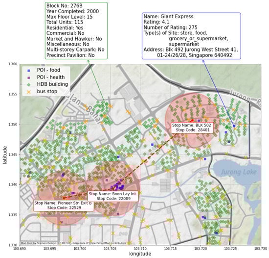
Figure 1. An example of three nodes centered around three bus stations Pioneer Stn Exit B, Boon Lay Int and BLK 502, as well as the distribution of HDB buildings and POIs in the area. The establishment attributes and coordinates of the HDB building BLK 276B and the POI Giant Express are shown as an example of what they will entail. The radius of the red circles is 500 m. Green diamonds represent HDB buildings, and blue and purple boxes represent POIs of type food and type health, respectively. Best viewed in colors.

The POI data contains data points of places that people have an interest in visiting for a certain purpose, which include but not limited to educational institutes such as schools or libraries, shopping places such as supermarkets or convenience stores, recreational places such as parks or bars. Generally speaking, the POI data can tell us what kind of activities are happening at the location. The HDB data contains data points of apartment buildings where people reside. In short, the HDB data shows where people are staying, while the POI data shows where people are visiting. Every day, people travel between these locations, forming a certain connection between them. With the bus routing data, the bus ridership data and the subway routing data, we hope to provide information on the system that supports these travels. Thus, this dataset has the potential to be used by researchers in the field for many different tasks that require knowledge of traffic, business and residential information of a city, especially when exploring their influence on each other.

We chose Singapore to conduct our study due to several characteristics of the city state. Singapore has a population of 5.686 million, and 100% of it is urban population; 80% of the residents live in HDB flats [67]. Meanwhile, walking and public transportation account for 78.2% of the modes of transport to school for students, and 67.6% of the modes of transportation to work for the working population. The average time for people to walk to school or work is about 8–10 min [68]. These characteristics make it possible to capture most of the Singaporean population distribution and population flow with the HDB housing and public transportation data.

Each attribute in the datasets may be gathered from one or a combination of the above sources. For example, the list of HDB buildings and their property information (e.g., block number, street name, number of storeys, year completed, total dwelling units, etc.) are first collected from the HDB Property Information published by Data.gov.sg [69], then we use their block numbers and street names to find the coordinates using OneMap API. Next, the building coordinates are used to match them with the planning area and region where they belong, using the planning area and region boundaries following the Master Plan 2019 published by the Urban Redevelopment Authority (URA) of Singapore [70]. The same data attribute may come from multiple sources to complement each other.

3.1. The POI Data

The POI dataset consists of 8672 POIs in Singapore collected from the Google Places API in September 2021. The API is provided by the Google Map platform, the No. 1 navigation app in Appstore SG. It contains detailed information on a wide range of POIs along with POI type information and customer reviews. To be comprehensive, we conducted searches for all 96 searchable POI types within each of the 55 planning areas in Singapore. Due to the limitation of the API, up to 60 search results per request will be returned, which means up to 60 POIs of each type within each planning area will be included. Each POI contains basic attributes such as names and coordinates, an overall user rating with the number of user ratings and several labels that describe the POI.

Each piece of POI data has three types of attributes as explained below.

• Identity Attributes The name, latitude and longitude are used to identify the POI and calculate the distance between different POIs or between a POI and a transport hub. They can also be used to find the planning areas and regions of the POI.
• Rating Attributes On Google Map, each user can give an integer rating among $[1,2,3,4,5]$ for a POI. The mean of all the user ratings, which is between $[1.0,5.0]$, will be the POI’s overall rating and shown in the Google search result to the public. If there are too few user ratings, the POI rating will be 0.
• Functionality Attributes There are a total of 104 POI functionality labels returned by the Places API. Each POI can have multiple labels, and some of them have partially overlapping concepts, e.g., convenience_store and food, home_goods_store and furniture_store. Some labels are parent concepts to another, e.g., school and secondary_school.

The detailed list of attributes can be found in Table 4.

Table 4. Attribute list of the POI data.

Attribute	Unit	Description	Example
name	-	the name of the POI	Crowne Plaza Changi Airport, Westwood Secondary School
lat	${}^{\circ }$	the latitude of the POI	$1.{34}^{\circ }$N
lng	${}^{\circ }$	the longitude of the POI	$103.{68}^{\circ }$E
pln_area	-	the planning area where this POI is located	Jurong West
region	-	the region where this POI is located	Central
rating	-	average Google Map user rating	$3.5$
n_rating	-	number of Google Map user rating	128
type	-	a list of POI type labels	store, logding, airport, school

3.2. The HDB Data

Singapore has one of the world’s best public housing systems. About 80% of Singapore residents live in units developed by the Housing and Development Board in Singapore, which are commonly referred to as HDBs. These units are located in apartment buildings that are grouped into large housing estates and are scattered all over Singapore. The distribution of HDB buildings and the number of units provide a good insight into the distribution of the residential population of Singapore, and information about their properties, such as the included facilities, can provide information on the type of services needed in the community.

From Data.gov.sg, we managed to retrieve a list of 12,442 HDB buildings existing in Singapore in September 2021. The distribution of the HDB buildings is shown in Figure 2. Each building has both identity attributes, building attributes and functionality labels, as explained below.

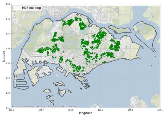
Figure 2. The distribution of HDB buildings in Singapore.

• Identity Attributes The identity attributes allow people to find the building on a map. They include block number, street, latitude and longitude of the HDB building. The planning area and region of the building are found using the coordinates.
• Building Attributes The building attributes describe the basic property of the building. They include the number of units in the building, the year when it was built and the number of storeys of the building.
• Functionality Labels The functionality labels describe the type of facilities included in the HDB building. The list of functionality labels include residential, commercial, market hawker, miscellaneous (Examples include admin office, childcare centre, education centre, Residents’ Committees centre), multistorey carpark and precinct pavilion. Similar to the POIs, these labels are non-exclusive.

The list of attributes are shown in Table 5.

Table 5. Attribute list of the HDB data.

Attribute	Unit	Description	Example
blk_no	-	the block number	652C
street	-	the street name	beach rd
lat	${}^{\circ }$	the latitude of the building	$1.{34}^{\circ }$N
lng	${}^{\circ }$	the longitude of the building	$103.{68}^{\circ }$E
pln_area	-	the planning area where this building is located	Jurong West
region	-	the region where this building is located	Central
year	-	the year when the building is completed	1984
units	-	number of dwelling units in the building	179
type	-	the functionality of the facilities in the building	residential

3.3. The Bus Routing Data

Singapore has one of the best public transport systems in the world. In the Deloitte City Mobility Index [71], which studies urban mobility performance in cites, Singapore scores the highest among all cities in all subcategories of performance and resilience. In particular, Singapore has the highest share of public transport among all travel modes, compared to other cities, such as Beijing, Shenzhen, New York or Paris, where other related studies are often based. This suggests that in Singapore, the public transport system has more influence on the land use-transport feedback cycle and must be taken into consideration when constructing a geospatial graph.

According to the Department of Statistics of Singapore, the two most popular transit modes are public buses and the Mass Rapid Transit/Light Rapid Transit (MRT/LRT) subways. From DataMall, we were able to collect information on 554 public bus routes with 5049 bus stations operating in Singapore during January 2020. The distribution of the bus stations is shown in Figure 3. Each piece of bus routing data has two types of attributes as explained below.

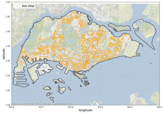
Figure 3. The distribution of bus stations in Singapore.

• Station Identity and Location Attributes The identity attributes include the coordinate, the identifier code and the name of the bus station. They can be used to find the bus station on the map. The planning area and the region of the station are also included.
• Routing Attributes The routing attributes include the bus line name, bus line direction, the sequence number of the bus stop and the distance of the stop to the starting station on the line. Note that bidirectional bus lines stop at different bus stops. These attributes detail how the bus stations are connected to each other by the lines.

The list of attributes can be found in Table 6.

Table 6. Attribute list of the public bus system data.

Attribute	Unit	Description	Example
stop_id	-	a 5-digit identifier code of the bus station	96109
lat	${}^{\circ }$	the latitude of the station	$1.{33}^{\circ }$N
lng	${}^{\circ }$	the longitude of the station	$103.{95}^{\circ }$E
pln_area	-	the planning area where this station is located	Jurong West
region	-	the region where this station is located	Central
line	-	the Service Number of the bus route	10
direction	-	1 for loop lines or the default direction, 2 for the reverse direction	1
sequence	-	the order of this station on this line in this direction	5
distance	km	distance from this station to the starting station	2.7

The routing and stop information allows u to build a graph that will be used to connect the areas of Singapore. We will explain in detail how to construct our nodes, graphs, features and node attractiveness in Section 4.2.

3.4. The Bus Ridership Data

Ridership information tells us about the number and direction of passenger flows at each bus station during different times of the day. From DataMall, we gather the monthly ridership information for 5018 out of the 5049 bus stations, which are collected for July, August and September 2021. As the passenger flow patterns during weekdays are usually different from those on weekends/holidays, the numbers are recorded separately for them. Each piece of the ridership data has three types of attributes as explained below.

Although this information will not be used in our site selection task, it is nonetheless a very interesting feature that has the potential to be used in other tasks, particularly those requiring temporal traffic data. Therefore, we decide to include the ridership data in our LTSG dataset for the use of other researchers in the field.

• Identity Attributes The identity attributes include the identifier code of the bus station, as well as the hour and the type of day of the record. The identifier codes of the bus station are the same as the ones used in Section 3.3. The hour is presented in a 24 h format. The type of day has two possible values: WD represents weekdays and H represents weekends or public holidays.
• Passenger Volume Attributes On a typical weekday or weekend/holiday, during the specific time period, the number of passengers tapping in and out of a station is recorded. They are averaged from the monthly numbers over July, August and September 2021.

The list of attributes can be found in Table 7 and an example is given. In the example, it is shown that on a typical weekday, an average of 695 passengers get on a bus at station 96109 between 15:00 to 15:59, and an average of 712 passengers get off a bus here during the same time.

Table 7. Attribute list of the bus ridership data.

Attribute	Unit	Description	Example
stop_id	-	a 5-digit identifier code of the bus station	96109
hour	-	hour of the record in 24-h format.	15
day	-	the type of day of the record.	WD
in	h${}^{-1}$	the average number of passengers departing from this station during the hour	695
out	h${}^{-1}$	the average number of passengers arriving at this station during the hour	712

3.5. The Subway Routing Data

In addition to the public bus system, the subway system, which includes LRT and MRT, is also an important part of the public transport system used by Singaporeans every day. From DataMall, we collect information of 9 subways routes with 166 subway stations operating in Singapore as of January 2020. Similar to the bus routing data, the subway routing data has two types of attributes as explained below.

• Identity and Location Attributes The identity attributes include coordinate, identifier code and name of the subway station. They can be used to find the bus station on the map. The planning area and the region of the station are also included.
• Routing Attributes The routing attributes include the subway line code and the sequence number of the station at the default direction. Note that bidirectional subway lines would stop at the same stations on both directions, which is different from bus lines. These attributes detail how the subway stations are connected to each other by the lines.

The list of attributes are shown in Table 8.

Table 8. Attribute list of the subway system data.

Attribute	Unit	Description	Example
stop_id	-	the official code of the station	EW28
name	-	name of the station	Pioneer
lat	${}^{\circ }$	the latitude of the station	$1.{33}^{\circ }$N
lng	${}^{\circ }$	the longitude of the station	$103.{95}^{\circ }$E
line	-	the name of the MRT/LRT line	EW
sequence	-	the order of this station on this line	28

4. Construction of the Geospatial Transport Graph with the LTSG Dataset

In this section, we are going to explain in detail how we make use of the datasets in Section 3 to construct this site-transportation graph for the site selection task. An overview of our GCN model is shown in Figure 4. Suppose we want to choose the optimal location to open a new store in Singapore. We first prepare a list of potential areas to choose from, which forms a set of nodes $\mathcal{V}=\{v_1,v_2,\dots ,v_i\},i=1,\dots ,N$, where N is the number of nodes (areas). These areas are connected to each other in a way defined by an adjacency matrix $\mathbf{A}\in {\mathbb{R}}^{N\times N}$, N being the number of nodes. For each node $v_i$, the feature ${\mathbf{x}}_i$ describes the environment within the node area, and the rating $y_i$ indicates how suitable is this area for the site selection. The optimal area would depend not only on the features of this area alone, but also its connection with the whole graph. Therefore, our site selection problem can be simplified to a task where we train a model to fit to the rating matrix $\mathbf{Y}=\{y_1,y_2,\dots ,y_i\}$, using the node feature matrix $\mathbf{X}=\{x_1,x_2,\dots ,x_i\}$ and an adjacency matrix $\mathbf{A}$.

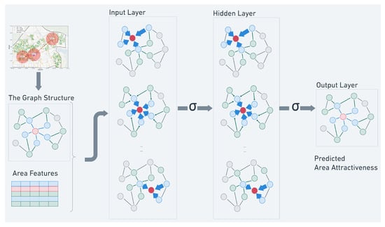
Figure 4. Visualization of the GCN model. The graph structure is built with the transportation network and shared throughout the model over layers. The input is multichannel node features and the output is single dimension node attractiveness.

The main issue in designing the model is how to enable information to propagate between the nodes to simulate the information propagation brought by people traveling between locations in real life. This can be tackled in two steps. The first is to determine the direction of the information flow with the construction of $\mathbf{A}$ described in Section 4.1.2, and the second is to determine the rules of the flow with the propagation rule described in Section 4.2.

4.1. Network Construction

As discussed before, in our geospatial transport graph $\mathcal{G}=(\mathcal{V},\mathcal{E})$, each node $v_i$ represents a potential area for site selection, and each edge $(v_i,v_j,a_{i,j})\in \mathcal{E}$ represents some form of connection between area $v_i$ and area $v_j$. The features of the potential areas can then be represented by a feature matrix $\mathbf{X}\in {\mathbb{R}}^{N\times K}$, where K is the number of features, and $N=\left|\mathcal{V}\right|$ is the number of nodes. The attractiveness of stores in this node can thus be represented by the attractiveness vector $\mathbf{y}\in {\mathbb{R}}^{N\times 1}$.

4.1.1. Node Construction

The first and most important step to construct the model is to define the nodes $\mathcal{V}$ on the graph. From Table 1, we can see that the size and shape of the node area depends on the task and network requirement. The nodes should cover an appropriate size of urban area, within which all POIs shared the geographic characteristics of this area, and all of them are considered similarly accessible. They should also have access to public transportation which links them together. In this study, we define the nodes as a circular area of radius $r_0=500$ m around a bus station. This makes each node comparable to a pedestrian shed, or ped-shed, a concept from the urban planning community, which emphasizes that an ideal neighborhood should provide one’s daily needs within walking distance [72]. It is defined as a circular area that surrounds an urban nucleus which is often a transport hub. A widely accepted radius of the area is around 400–800 m, corresponding to 5–10 min of walking [73,74,75].

The radius of 500 m is carefully selected based on both theoretical works and real-world data. In [76], a 400-m rule is proposed as the optimal radius for ped-sheds and proved to be a pattern presented in cities over the world in their natural development processes. From the analysis of location-based services data in [10], around 70% of the visitors to POIs in the center of New York City come from within a distance of 500 m. According to public transportation statistics [68], in Singapore, the average distance people would walk to work/home or to a transport hub is around 584 meters. This implies that the nodes as defined above fit the pattern of the movement and living situation of average Singaporeans and thus best for both feature construction and attractiveness evaluation.

In the following sections of the paper, the nodes will be denoted as $\mathcal{V}=\{v_1,v_2,\dots ,v_i\}$, and the central bus stations will be denoted as $\{{\nu }_1,{\nu }_2,\dots ,{\nu }_i\}$ accordingly. Because only 5045 out of the 5049 bus stations in our dataset are located within Singapore, $\left|\mathcal{V}\right|=5045$. For any settlement p on the map, if p is located inside the node area $v_i$, we will denote it as $p\in v_i$. By this definition, the set $\mathcal{V}$ covers a total area of 434 km${}^2$, which is $76.8\%$ of the total urban land area of Singapore [77], as shown in Figure 5.

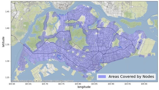
Figure 5. The areas covered by all of the nodes defined according to Section 4.1.1. As shown in the figure, the nodes covered most urban areas in Singapore. The areas not included are either natural reserves (the green areas) or industrial areas (the bottom island and the areas on the right).

4.1.2. Adjacency Matrix Construction

The adjacency matrix describes the edges of the graph, i.e., the transportation connection between areas. In accordance with the Singaporean public transportation statistics [68] cited above, walking and public transportation comprise the majority of the transportation methods used by Singaporeans. Therefore, we will construct the edges between nodes based on transportation, which includes working and public transportation. Finally, we settle on the combination of two adjacency matrices, highlighting connection by walking, public bus and subway, respectively.

• Walking-Based Adjacency Matrix

  $${\mathbf{A}}_{1,i,j}=\left\{\begin{array}{cc}1,\hfill & \mathrm{if}{\nu }_j\in v_i,\hfill \\ 0,\hfill & \mathrm{otherwise}.\hfill \end{array}\right.$$

  (1)
  For two nodes $v_i$ and $v_j$, if the distance between their central bus stations ${\nu }_i$ and ${\nu }_j$ is smaller than $r_0$, they are considered connected and vice versa. This also means that the two areas overlap with each other significantly. This adjacency matrix describes whether two nodes are connected by means of walking. The implication is that, if a potential customer is nearby, it is equally convenient for them to visit these areas.
• Bus-Based Adjacency Matrix

  $${\mathbf{A}}_{2,i,j}=\left\{\begin{array}{cc}1,\hfill & \mathrm{if}{\nu }_i\mathrm{and}{\nu }_j\mathrm{are}\mathrm{on}\mathrm{the}\mathrm{same}\mathrm{bus}\mathrm{route},\hfill \\ 0,\hfill & \mathrm{otherwise}.\hfill \end{array}\right.$$

  (2)
  For two nodes $v_i$ and $v_j$, if their central bus stations ${\nu }_i$ and ${\nu }_j$ are on the same bus route, they are considered connected. This adjacency matrix described whether two nodes have a direct bus connection.
• Subway-Based Adjacency Matrix

  $${\mathbf{A}}_{3,i,j}=\left\{\begin{array}{cc}1,\hfill & \mathrm{if}{v}_i\mathrm{and}{v}_j\mathrm{are}\mathrm{on}\mathrm{the}\mathrm{same}\mathrm{subway}\mathrm{route},\hfill \\ 0,\hfill & \mathrm{otherwise}.\hfill \end{array}\right.$$

  (3)
  For two nodes $v_i$ and $v_j$, if they contain subway stations on the same route, they are considered connected. This adjacency matrix indicates whether two nodes have a direct subway connection. The bus and subway adjacency matrices correspond to a traditional P-space transport network, which has proven useful in human mobility studies [78,79].

With a combination of these three matrices, we can capture the multimodal transport links between nodes. The implication is that a potential customer in node ${\nu }_i$ can reach any areas in the node’s neighborhood $\mathcal{N}\left({\nu }_i\right)=\left\{{\nu }_j\right|{\mathbf{A}}_{i,j}>0\}$ without changing means of transportation [78,79]. Based on the adjacency matrix used in the model, we proposed two GCN models: GCN-walking and GCN-combine. For GCN-walking, $\mathbf{A}={\mathbf{A}}_0+{\kappa }_1{\mathbf{A}}_1$ and for GCN-combine, $\mathbf{A}={\mathbf{A}}_0+{\kappa }_1{\mathbf{A}}_1+{\kappa }_2{\mathbf{A}}_2+{\kappa }_3{\mathbf{A}}_3$, where ${\mathbf{A}}_0$ denotes the self-connection matrix ${\mathbf{A}}_0=\mathbf{I}$ to emphasize the local influences. The hyperparameters ${\kappa }_1$, ${\kappa }_2$, ${\kappa }_3$ can adjust the weights between the two methods of transportation and the node’s self-connection.

4.1.3. Feature Construction

With the above definition of nodes $\mathcal{V}$ and the adjacency matrix $\mathbf{A}$, we can now construct the node feature matrix $\mathbf{X}$ by giving each node area a feature representation. It will include a summary of both the HDB and POI information located within the area:

• The HDB Features From the HDB data, we can construct an HDB feature matrix ${\mathbf{X}}_H\in {\mathbb{R}}^{N_H\times F_H}$, with $N_H$ and $F_H$ denoting the number and the feature number of HDB building properties, including the number of storeys, the number of units, year of completion and the type of facilities in the building. For each node $v_i$, we aggregate the HDB building properties for all HDB buildings inside the area $v_i$ as its features. For a set of HDB buildings $\{h_1,h_2,h_i\}$, we can define a binary incidence matrix $B_H\in {\mathbb{R}}^{N\times N_H}$, which describes whether a HDB building $h_j$ is located in area $v_i$.

  $${\mathbf{B}}_{H,i,j}=\left\{\begin{array}{cc}1,\hfill & \mathrm{if}{h}_j\in v_i,\hfill \\ 0,\hfill & \mathrm{otherwise}.\hfill \end{array}\right.$$

  (4)
  Taking into account the number of HDB buildings in the area, we normalize ${\mathbf{B}}_H$ into ${\widehat{\mathbf{B}}}_H={\mathbf{D}}_H^{-1}{\mathbf{B}}_H$, where ${\mathbf{D}}_H$ is a diagonal matrix, and ${\mathbf{D}}_{H,i,i}={\sum }_j{\mathbf{B}}_{H,i,j}$ is the total number of HDB buildings in node area $v_i$. Then, the HDB feature matrix can be calculated as ${\mathbf{X}}_{\mathrm{HDB}}={\widehat{\mathbf{B}}}_H{X}_H\in {\mathbb{R}}^{N\times F_H}$.
• The POI Features The number of different types of POI in an area indicates the type of activity people do in this area. It can also reveal information such as the level of business competition or the level of inter-business attractiveness (for example, there are often restaurants around a movie theater, thus restaurants can be considered attracted by movie theaters). Some of the POI types are highly specific services such as casino or cemetery, each with fewer than 10 establishments in the country, thus not providing enough data for analysis. Among the 104 labels, we choose 53 labels which are the most commonly distributed across Singapore and count the number of POIs under each label for each node. Suppose we have $N_P$ number of POIs, forming a set of POIs $P=\{p_1,p_2,\dots ,p_{N_P}\}$. $P^t\subset P$ contains all POIs of type t, e.g., store, logding, finance, school. $P_{v_i}\subset P$ contains all the $p\in v_i$ and $P_{v_i}^t=P_{v_i}\cap P^t$. The POI feature matrix will be ${\mathbf{X}}_P\in {\mathbb{R}}^{N_P\times T}$, with $T=53$. For a set of POIs $\{p_1,p_2,p_i\}$, we can define a binary incidence matrix ${\mathbf{B}}_P\in {\mathbb{R}}^{N\times N_P}$

  $${\mathbf{B}}_{P,i,j}=\left\{\begin{array}{cc}1,\hfill & \mathrm{if}{p}_j\in v_i,\hfill \\ 0,\hfill & \mathrm{otherwise}.\hfill \end{array}\right.$$

  (5)
  This can be normalized in the same way as ${\mathbf{B}}_H$, so that ${\widehat{\mathbf{B}}}_P={\mathbf{D}}_P^{-1}{\mathbf{B}}_P$ where ${\mathbf{D}}_{P,i,i}={\sum }_j{\mathbf{B}}_{P,i,j}$ is the total number of POIs in node $v_i$. Thus, the node feature matrix can be calculated as $\mathbf{X}={\widehat{\mathbf{B}}}_P{\mathbf{X}}_P\in {\mathbb{R}}^{N\times T}$. Therefore, ${\mathbf{X}}_{\mathrm{POI}}={\mathbf{B}}_P{\mathbf{X}}_P$ can be viewed as the distribution of different types of POIs in the node area. Each row in the matrix represents the frequency of each types of POIs within a node area.

4.1.4. Label Construction

One major challenge in the store site selection problems lies in the difficulty to judge the goodness of the decisions. Needless to say, there are many location irrelevant factors that contribute to the success of a business, and it is almost impossible to separate the location relevant factors from the irrelevant ones. In this study, we will use the area store rating to evaluate the attractiveness of the area.

In the Google Map app, each user can give a review score $s\in \{1,2,3,4,5\}$ to a POI. The final user rating of the POI, which is the one shown to all users, is the mean of all user ratings $\overline{s}\in (1.0,5.0)$, which we will normalize to $\widehat{s}\in (0.0,1.0)$. If a store has more than 10 ratings, we treat it as a “qualifying store” with a consistent performance.

The attractiveness of a node will then be calculated for all the nodes with more than 10 qualifying stores by averaging the rating of all stores in the area, weighted by the number of ratings for each store. While each single user rating reflects the overall user experience, that can be highly personal; with enough ratings summarizing over multiple stores within an entire area, we believe it can be used to judge whether the area gives a positive leverage to the performance of stores. In our dataset, the mean number of ratings per POI is 313.96, which should be enough to balance out the impact of store-specific, location irrelevant factors.

If the rating and the number of ratings for a store p is ${\widehat{s}}_p$ and $w_p$, respectively. For each node, the attractiveness is calculated as

$${\mathbf{y}}_i=\frac{{\sum }_{p\in v_i}{\widehat{s}}_p·w_p}{{\sum }_{p\in v_i}{w}_p}.$$

(6)

4.2. Model Structure

Once we have constructed the geospatial transport graph, we can proceed to the next step, which is defining the information propagation rules between nodes. The GCN model proposed in [44] introduces a simple yet powerful approximation of the spectral graph convolution method, which allows information to be aggregated from neighboring nodes at each layer. This process includes the multiplication of the outputs with the graph Laplacian. Each multiplication can be seen as replacing the current node features with an aggregation of its neighbors. With our geospatial graph, the neighbor consists of the node itself, its nearby nodes, and nodes connected to it by bus. For our task, a two-layer GCN model is chosen. The prediction of rating $\widehat{\mathbf{y}}$ can be expressed as:

$$\widehat{\mathbf{y}}={\sigma }_1\left(\widehat{\mathbf{A}}{\sigma }_0\left(\widehat{\mathbf{A}}\mathbf{X}{\mathbf{W}}^{\left(0\right)}\right){\mathbf{W}}^{\left(1\right)}\right),$$

(7)

where

• $\widehat{\mathbf{A}}$ is a normalized adjacency matrix. $\widehat{\mathbf{A}}={\mathbf{D}}^{-\frac{1}{2}}\mathbf{A}{\mathbf{D}}^{-\frac{1}{2}}$ and ${\mathbf{D}}_{ii}={\sum }_j{\mathbf{A}}_{ij}$ being the degree matrix that signifies the accessibility of node $v_i$. For GCN-walking, $\mathbf{A}={\mathbf{A}}_0+{\kappa }_1{\mathbf{A}}_1$ and for GCN-combine, $\mathbf{A}={\mathbf{A}}_0+{\kappa }_1{\mathbf{A}}_1+{\kappa }_2{\mathbf{A}}_2$. The self-connections are added to emphasize the node’s own features.
• ${\mathbf{W}}^{\left(0\right)}$ and ${\mathbf{W}}^{\left(1\right)}$ are the trainable weights at the first and second layer.
• $\mathbf{X}\in {\mathbb{R}}^{N\times F}$ is the feature matrix, with N being the total number of bus stations, and F being the number of features. Each row of $\mathbf{X}$ is a feature representation of the local environment of a node area.
• The leaky ReLU function is chosen as the activation function ${\sigma }_0(·)$ at the hidden layer to adds non-linearity in the model, and the sigmoid activation function is chosen for the output layer ${\sigma }_1(·)$ to make sure the predicted attractiveness lies within the range of (0.0, 1.0).

4.3. Loss Function

The smooth L1 loss is used in the training as a balance between L2 and L1 loss. One thing to be noted is that the area store rating would be 0 if there are not enough qualifying stores in the area. In this case, a rating of $y_i=0$ does not truly reflect the attractiveness of POIs in $v_i$, and instead would be masked as a missing ground truth value. In the loss function, we only calculate for the valid ground truth $y_i>0$. Therefore, the final loss function is

$$loss=L(y_i,{\widehat{y}}_i)+\lambda \sum w^2,$$

(8)

where the first term

$$L(y_i,{\widehat{y}}_i)=\left\{\begin{array}{cc}0.5|y_i-{\widehat{y}}_i{|}^2/\beta \hfill & \mathrm{if}{y}_i=0\mathrm{and}|y_i-{\widehat{y}}_i|<\beta ,\hfill \\ |y_i-{\widehat{y}}_i|-0.5\beta \hfill & \mathrm{otherwise}.\hfill \end{array}\right.$$

(9)

This evaluates the difference between our prediction and the ground truth. The hyperparameter $\beta$ is used to control the threshold where the loss function switches between L2 and L1 loss. The second term $\lambda \sum w^2$ is an L2 regularization term to prevent overfitting, where $\lambda$ and w are the regularization rate and the weights to be trained, respectively.

5. Experiment

In this section, we evaluate the effectiveness of our GCN model in real-world examples by applying the algorithm described in Section 4 on the LTSG dataset described in Section 3. We predict the attractiveness of a set of nodes, providing POI distribution and the housing information of these areas and the transportation network connecting them.

The attractiveness of nodes reflects the overall performance of stores in this area, and in return, whether this area is a good location for store placement. If a model can accurately predict the actual attractiveness, it demonstrates the ability to understand how the distribution of commercial and residential establishments influence the store performance, which will be a great aid for site selection.

5.1. Experimental Settings

To avoid data leaking caused by overlapping nodes, we divide our data into training, testing and validation sets based on their geographic locations. The average distance between two nearest bus stations is 46 m, much smaller than $r_0$, which means there are many overlapping nodes with similar features and attractiveness. To make sure these nodes do not cause data leaking between training and testing sets, the data splitting scheme must be able to make sure geographically close nodes are separated. The boundaries are chosen based on the administrative divisions of Singapore, which are widely used in government ministries and departments as guidance. There are two basic levels of administrative division in Singapore, namely, regions and planning areas, and we prepare two data split schemes based on them. The details of the two schemes are shown in Figure 6 and Table 9.

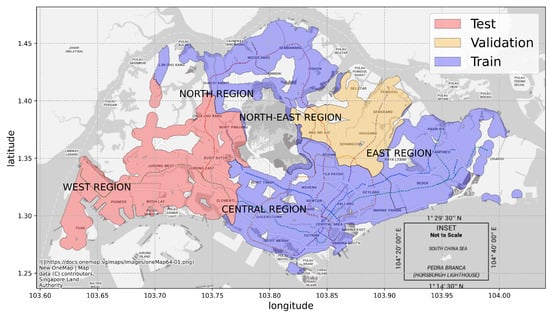
Figure 6. Nodes in the red area (West Region) are used for testing, nodes in the orange area (Northeast Region) are used for validation, and nodes in the blue area (North Region, East Region and Central Region) are used for training. Best viewed in colors.

Table 9. Sizes of the training, testing and validation set in the two data split schemes. The lists of planning areas in each set are shown in Appendix A.

Scheme		Training	Testing	Validation
	# of planning areas	30	9	11
1	# of nodes	2678	1281	1086
	planning areas	See Appendix A
	# of regions	3	1	1
2	# of nodes	1359	2904	782
	regions	North, East, Central	West	North-East

According to the Master Plan 2019, the land area of Singapore can be divided into 5 regions and further into 55 planning areas. Among the 55 planning areas, 5 of them do not contain any nodes. Therefore, in Scheme 1, we segment our graph into 50 sub-graphs according to the planning area boundaries and randomly select 30 planning areas for training, 9 for testing and 11 for validation. Nodes will be put into the respective set according to their geographic location. Similarly, in Scheme 2, we segment our graph into five sub-graphs based on the region boundaries and choose the North, East, and Central Region for training, the West Region for testing and the Northeast Region for validation.

There are two learning approaches that we use: transductive and inductive learning. This is to test our model under different scenarios. Transductive learning targets more specific cases where we make predictions on a masked segment of a known graph, while inductive learning tries to generalize from testing cases and makes predictions on completely new graphs.

• Transductive Learning In transductive learning, during the training process, we predict the attractiveness of nodes in the testing planning areas or regions based on the housing information and public transport network of all Singapore. In the transductive setting, the model has access to the features and structures of the entire graph during training and testing, but the ground truths of the respective nodes in the training, testing and validation sets will masked. In Scheme 1, we can test if our model is able to fill in the attractiveness of maps based on the rest of the map at the planning area level. In Scheme 2, we can test if it can do the same at the region level.

  -

  During training: input ${\mathbf{A}}_{total}\in {\mathbb{R}}^{N_{total}\times N_{total}}$ and ${\mathbf{X}}_{total}\in {\mathbb{R}}^{N_{train}\times F}$, train on ${\mathbf{y}}_{train}\in {\mathbb{R}}^{N_{train}\times C}$.

  -

  During testing: input ${\mathbf{A}}_{total}\in {\mathbb{R}}^{N_{total}\times N_{total}}$ and ${\mathbf{X}}_{total}\in {\mathbb{R}}^{N_{total}\times F}$, predict ${\mathbf{y}}_{test}\in {\mathbb{R}}^{N_{test}\times C}$.

• Inductive Learning The GCN model as described in Section 4.2 is a spectral-based model, which usually requires knowledge of the entire graph beforehand, thus suffering from the inability to be transferred to a new graph [50,51,59]. However, as mentioned in [56], this GCN can also be interpreted from a spatial perspective that aggregates node features from the first-order neighbors of the central node [49,56]. Therefore, it is appropriate to apply it on segments of the entire graph, in this case one or more planning areas or regions in Singapore, essentially forming an inductive learning task where we try to predict the attractiveness of areas on a previously unseen map. In the inductive setting, the model has no access to the features and structures of the testing and validation sub-graphs. The training, testing and validation sets will be considered as individual graphs, and only their internal node connections will be used to make predictions. In Scheme 1, we can test the generalizability of our model to incomplete maps with some unknown parts. In Scheme 2, as the regions vary greatly in their land use design, we can test the ability of our model to be generalized to a different type of area, even if it has no prior knowledge of the area before.

  -

  During training: input ${\mathbf{A}}_{train}\in {\mathbb{R}}^{N_{train}\times N_{train}}$ and ${\mathbf{X}}_{train}\in {\mathbb{R}}^{N_{train}\times F}$, train on ${\mathbf{y}}_{train}\in {\mathbb{R}}^{N_{train}\times C}$.

  -

  During testing: input ${\mathbf{A}}_{test}\in {\mathbb{R}}^{N_{test}\times N_{test}}$ and ${\mathbf{X}}_{test}\in {\mathbb{R}}^{N_{test}\times F}$, predict ${\mathbf{y}}_{test}\in {\mathbb{R}}^{N_{test}\times C}$.

5.2. Baselines

We will be comparing the results of our model against the following three baseline methods:

• Linear Regression (LR) Linear regression tries to fit a linear equation to the data in the form of $\widehat{y}=X\beta +ϵ$ where $\beta$ and $ϵ$ are $K\times 1$ and $N\times 1$ vectors, respectively. It will calculate the value of $\beta$ and $ϵ$ by minimizing the residual sum of squares between $\widehat{y}$ and the ground truth y of the training set. We adopt the LinearRegression implementation from the sklearn.linear_model module.
• Random Forest Regression (RF) The random forest regression fits a decision tree on the training set. In each split, all features and all samples are examined to find the best split to minimize the squared error in the prediction until the leaves are pure. This will be repeated 100 times, and the final prediction will be the average of the result of the 100 decision trees. We adopt the RandomForestRegressor implementation from the sklearn.ensemble module.
• Multilayer Perceptron (MLP) We also compare our model performance against a multilayer perceptron with 1 hidden layer with 16 units. The formula of the MLP prediction is $\widehat{\mathbf{y}}=\sigma \left(\sigma \left(\mathbf{X}{\mathbf{W}}^{\left(0\right)}\right){\mathbf{W}}^{\left(1\right)}\right)$, where $\mathbf{X}$ is the same feature matrix as used in the GCN model, ${\mathbf{W}}^{\left(0\right)}$ and ${\mathbf{W}}^{\left(1\right)}$ are trainable weights and the activation functions $\sigma (·)$ are LeakyReLU and sigmoid at the first and second layer, respectively. Compared to the formulation of the GCN in Equation (7), we can easily see that the MLP can be interpreted as a GCN with only self-connections between nodes.

Due to the limitation of the LR and RF models, they can only train under the inductive setting, and MLP can perform both inductive and transductive training. All of these baseline models consider only the node features and are incapable of making use of the graph structure. For site selection problems, this means they can only take into account the local features of an area and cannot weigh in the influence of connected areas.

5.3. Evaluation Metrics

To evaluate the performances of these methods, we use the following metrics to evaluate the prediction results:

The mean squared error (MSE):

$$\mathrm{MSE}(\mathbf{y},\widehat{\mathbf{y}})=\sum _i{d}_i^2.$$

(10)

The mean absolute error (MAE):

$$\mathrm{MAE}(\mathbf{y},\widehat{\mathbf{y}})=\sum _i{d}_i.$$

(11)

The mean absolute percentage error (MAPE):

$$\mathrm{MAPE}(\mathbf{y},\widehat{\mathbf{y}})=\sum _i\frac{d_i}{y_i}.$$

(12)

All of these metrics measure the closeness of our predicted node attractiveness to the ground truth, with MSE being more sensitive to outliers, MAE less so, and MAPE being MAE normalized by the ground truths, thus taking the percentage of the deviation of our prediction from the ground truth into consideration. Since an attractiveness of $y_i=0$ results from having no existing stores in the area and does not reflect the actual attractiveness of the area should there be a store, we will include these nodes in the training but treat them as having no ground truth $y_i$. Therefore,

$$d_i=\left\{\begin{array}{cc}|y_i-{\widehat{y}}_i|\hfill & \mathrm{if}{y}_i>0,\hfill \\ 0\hfill & \mathrm{otherwise}.\hfill \end{array}\right.$$

(13)

5.4. Results

We train on a two-layer GCN model with the hidden layer output dimension being eight, the starting learning rate of $0.05$, and the dropout rate set to $0.0$. A sigmoid activation function is used in the output layer to keep the attractiveness in the 0–1 range. Both GCN and MLP are trained for a maximum of 500 epochs, with early stopping when the validation loss has not seen improvement in the last 10 epochs. The list of hyperparameters is presented in Table 10.

Table 10. List of hyperparameters in the neural networks.

Hyperparameter	GCN	MLP
${\kappa }_1$	1.00	-
${\kappa }_2$	1.00
hidden layer units	8	8
learning rate	0.05	0.05
dropout rate	0.00	0.00
l2 reg. $\lambda$	$1\times {10}^{-4}$	$1\times {10}^{-5}$

Two types of GCNs are tested, each with a different adjacency matrix, constructed in Section 4.1.2. GCN-walking uses $\mathbf{A}={\mathbf{A}}_0+{\kappa }_1{\mathbf{A}}_1$, and GCN-combine uses $\mathbf{A}={\mathbf{A}}_0+{\kappa }_1{\mathbf{A}}_1+{\kappa }_2{\mathbf{A}}_2$, with ${\kappa }_1={\kappa }_2=1$. As discussed before, these matrices represent node connections by walking and a combination of walking and bus. This is to compare the influence of different transport modes. The results of the experiment are shown in Table 11 and Table 12, respectively.

Table 11. Results—Scheme 1 (training/testing/validation set split by area). The best results are shown in bold text.

Setting Model	Transductive			Inductive
	MSE	MAE	MAPE	MSE	MAE	MAPE
RF	-	-	-	0.01331	0.04929	0.05994
LR	-	-	-	0.01045	0.04860	0.05883
MLP	0.00135	0.02698	0.03446	0.00135	0.02696	0.03445
GCN-walking	0.00116	0.02575	0.03169	0.00110	0.02458	0.03034
GCN-combine	0.00111	0.02545	0.03133	0.00110	0.02465	0.03045

Table 12. Results—Scheme 2 (training/testing/validation set split by region). The best results are shown in bold text.

Setting Model	Transductive			Inductive
	MSE	MAE	MAPE	MSE	MAE	MAPE
RF	-	-	-	0.02486	0.08414	0.09990
LR	-	-	-	0.02241	0.07572	0.08929
MLP	0.00315	0.03280	0.04120	0.00325	0.03288	0.04127
GCN-walking	0.00226	0.03122	0.03809	0.00216	0.03278	0.04030
GCN-combine	0.00264	0.03478	0.04249	0.00207	0.03064	0.03759

The results show that the two GCN models, both GCN-walking and GCN-combine, give the most accurate prediction, achieving the lowest MSE, MAE and MAPE among all the methods. The non-neural network methods, including random forest regression and linear regression, perform poorly, resulting in MSEs that are a magnitude larger than other methods. This is due to these simple models lacking in expressivity. The relationship between the distribution and function of HDB buildings and POIs, and the attractiveness of the stores in the area are too complex for them to handle. Compared with another neural network model, GCN-walking and GCN-combine perform better than MLP in both schemes and training settings. For Scheme 1, in the inductive setting, the best performing model is GCN-walking, and in the transductive setting, the best performing model is GCN-combine. For Scheme 2, in the inductive setting, the best performing model is GCN-combine and in the transductive setting, the best performing model is GCN-walking. This proves that the attractiveness of stores in the area is not only influenced by local features but also its traffic connections to other areas.

Under transductive training settings, the three models make predictions based on knowledge of the full map. However, MLP is in fact unable to make use of this knowledge because it only considers each node’s own features. Under inductive training settings, the model will be tested on areas (new graphs) it has never seen before, including 10 planning areas in Scheme 1 and the entire West Region in Scheme 2. Comparing the results of inductive vs. transductive training settings, we have shown that our method does not require previous knowledge of the graphs in the training stage. The implication is that, even in new areas where the attractiveness labels are not available, for example, areas where no stores have been set up, or a city where no data on store performance can be obtained, as long as we have the traffic connection network as well as the local features, we can make predictions with a model trained with data from elsewhere. However, comparison of the results of Scheme 1 vs. Scheme 2 shows that the performance of our model decreases when the size of the testing area (in terms of the land area covered) increases, even though it still gives more accurate attractiveness predictions than other baseline methods. This is a possible limitation on the areas in which the model can be applied.

It is worth noting that GCN-combine, which takes into both walking and public transport connections, does not always perform better than GCN-walking. This suggests that public transport connections are not always a strong factor in area attractiveness. For example, in Scheme 1 under inductive training, the testing areas are relatively small, containing mostly neighborhoods of similar functionalities, so the public transport system contributes little to connection within the area. In comparison, in Scheme 2, the testing region is much larger and usually contains areas of different functionalities, such as business centers, residential areas and industrial areas. People need to take the public transport to travel between them, thus the public transport connection added by GCN-combine becomes more important.

6. Case Study: Site Selection in the Jurong West Planning Area

To demonstrate how our model can better predict the attractiveness of areas using the transport network and to examine some of the limitations in the current model, we conducted a short case study in the Jurong West planning area. We will discuss both the successful and unsuccessful cases of our prediction, and their reasons.

6.1. Overview of Jurong West

Jurong West is one of the 55 planning areas of Singapore, located in the West Region of Singapore. It borders five other planning areas: Tengah, Jurong East, Boon Lay, Pioneer and Western Water Catchment. In data split Scheme 1, Jurong West is one of the 10 planning areas in the testing set. Jurong West is primarily a residential area, with a population of 262,730 [80]. There are 106 bus lines (counting variants and opposite directions of the same line) and 1 subway line going through the planning area. Most business activities are located at or near the Boon Lay subway station, as can be inferred from Figure 7.

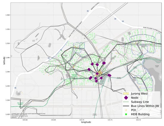
Figure 7. The distribution of HDB buildings, POIs, bus and subway lines and existing nodes that contain more than 10 stores in the Jurong West planning area.

6.2. Evaluation of Prediction Results

Under data split Scheme 1 (by planning area) and the transductive training setting, we can see from Figure 8 that MLP is unable to make good prediction for the circled nodes, probably due to lack of POI data, but our GCN is able to more accurately predict their attractiveness by using its connection to other areas via bus lines.

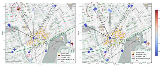
Figure 8. An example of a successful prediction in our GCN model. The two nodes in the circled area have more accurate attractiveness predictions from GCN (right) than from MLP (left). Both nodes locate in a residential area with no POIs nearby, but they are conveniently connected to other areas, especially the Jurong Point business hub, through bus lines. The poor MLP performance might be due to the lack of local POI information within the node area, but GCN can easily amend this issue by aggregating this information from the neighboring nodes.

However, under the same setting, in the cases demonstrated in Figure 9, the GCN model fails to predict the attractiveness for the node on the right. The two nodes in the circle area are 50 m from each other and share the same bus lines. Thus, both their local geographic features and transport connection are similar in our model, and they receive similar attractive predictions. But looking closely, they are on the opposite side of a main road, which does not allow easy commuting between them on foot. The estimated travel time between them by walking is 7 min. Moreover, the bus lines they share are a circular line: on bus line 79, Stop 21351 (on the left) is 1 stop away from Jurong Point, the main business hub, while Stop 21359 (on the right) is 49 stops away from it.Therefore, their actual attractiveness for store placement is quite different, a fact our model failed to predict. This highlights two limitations in our current model:

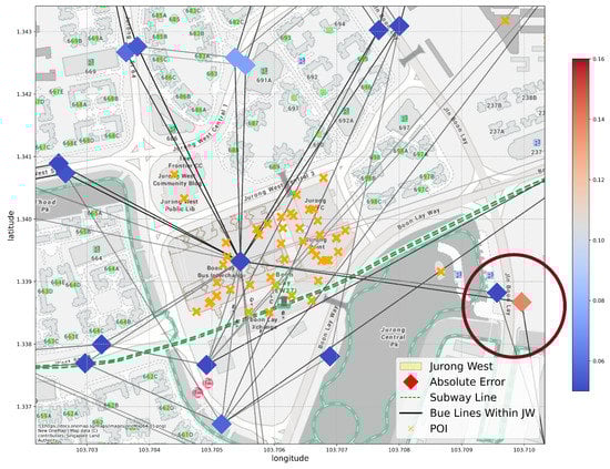
Figure 9. An example of an unsuccessful prediction in our GCN model.The two nodes in the circled area are centered around Stop 21351 (left) and Stop 21359 (right). They appear to share similar local geographic features and transport connections, but the circumstances are quite different.

1.

In the public transport graphs, all bus stations on the same line are considered connected despite the sequential difference between them; in the walking distance graph, the connection between areas is determined by Euclidean distance. Both of the connection types reflect a level of connection, but they do not correspond to the actual travel time, which seems to be an important factor in people’s travel decisions in real life, and the current edges fail to reflect this.

2.

The current graph we built is undirected. However, the human flow through bus and subway lines is directed, especially for circular lines. This makes the model unable to determine the direction of information propagation during convolution, thus unable to distinguish stops at different sequence or direction of the same line.

7. Conclusions

In this study, we tackle the problem of selecting the most attractive area for storefront placement by predicting the attractiveness of areas based on the local geographical features and its connection to other areas.

We accomplish this by first building a geospatial transport graph with the proposed Land and Transport Singapore (LTSG) dataset, which consists of comprehensive public housing, public transportation and points of interest information for the entirety of Singapore. This dataset can provide great insight into the population distribution and transport flow of Singapore and how they influence the land use around the city. This dataset has the potential to be used for various tasks besides site selection tasks, e.g., traffic demand prediction, and land use classification. We also demonstrate how to integrate different types of land use data with traffic data, which are often treated separately, with the construction of the geospatial transport graph.

We then build two geospatial GCN models from the above dataset, one based purely on proximity (GCN-walking) and the other based on both proximity and transportation (GCN-combine), to predict the area attractiveness for store site selection in Singapore. Our models give more accurate predictions compared to methods that are limited to use only local features, as demonstrated by the results. This proves that the area attractiveness is not only influenced by local features but also features of other areas if people can travel between them conveniently. The GCN models enable us to exploit the traffic network and make use of the information on greater parts of the map, which cannot be achieved by previous non-GCN methods. This not only improves the overall prediction accuracy but also allows the models to be used in more scenarios than those methods. For example, the GCN models can generate reliable attractiveness predictions for node areas where local features are lacking, as shown in the case study, which has not been possible. Furthermore, our model can be conveniently generalized to entire new regions, which would be of great help when looking for the location for a store in a new region with no prior knowledge.

Based on the previous discussions, our plan for the future work includes:

• Design a better GCN model that will allow us to process directed transport graphs, as well as adjusting the weights based on the connection strength between areas.
• Design a multi-layer geospatial transport graph that can better model the interaction between areas at different levels and for different transport modes. In addition, include travel time as one of the deciding factors for the connection between areas.
• Expand the LTSG dataset to include demographic data, land use data, real estate price data and road network data. This will not only provide more geographic and transport information for site selection tasks but also open the possibilities of the dataset for other tasks such as real estate price prediction, land use planning and transport planning.

Appendix A.1. List of Planning Areas in the Training Set

• Rochor
• Outram
• Marina South
• Straits View
• Museum
• Orchard
• Queenstown
• Bukit Timah
• Southern Islands
• Jurong East
• Boon Lay
• Tuas
• Choa Chu Kang
• Tengah
• Lim Chu Kang
• Newton
• Novena
• Central Water Catchment
• Bukit Batok
• Sungei Kadut
• Woodlands
• Sembawang
• Yishun
• Toa Payoh
• Bishan
• Geylang
• Paya Lebar
• Seletar
• Tampines
• Marine Parade

Appendix A.2. List of Planning Areas in the Testing Set

• Singapore River
• Tanglin
• Jurong West
• Western Water Catchment
• Bukit Panjang
• Serangoon
• Sengkang
• Hougang
• Bedok

Appendix A.3. List of Planning Areas in the Validation Set

• Kallang
• Downtown Core
• Bukit Merah
• River Valley
• Clementi
• Pioneer
• Mandai
• Ang Mo Kio
• Punggol
• Pasir Ris
• Changi

References

- Strauss, S.D. The Small Business Bible: Everything You Need to Know to Succeed in Your Small Business; Wiley: Hoboken, NJ, USA, 2012. [Google Scholar]
- Steingold, F.S. Legal Guide for Starting & Running a Small Business; Nolo: Berkeley, CA, USA, 2011; p. 448. [Google Scholar]
- Moniruzzaman, M.; Páez, A. Accessibility to transit, by transit, and mode share: Application of a logistic model with spatial filters. J. Transp. Geogr. 2012, 24, 198–205. [Google Scholar] [CrossRef]
- Healey, M.J.; Ilbery, B.W. Location and Change: Perspectives on Economic Geography; Oxford University Press: New York, NY, USA, 1990; pp. 343–354. [Google Scholar] [CrossRef]
- Kaufmann, P.J.; Donthu, N.; Brooks, C.M. Multi-Unit Retail Site Selection Processes: Incorporating Opening Delays And Unidentified Competition. J. Retail. 2000, 76, 113–127. [Google Scholar] [CrossRef]
- Ghosh, A.; Craig, C.S. A Franchise Distribution System Location Model. J. Retail. 1991, 67, 466. [Google Scholar]
- Achabal, D.D.; Gorr, W.L.; Mahajan, V. MULTILOC: A Multiple Store Location Decision Model. J. Retail. 1982, 58, 5. [Google Scholar]
- Quan, X.; Wenyin, L.; Dou, W.; Xiong, H.; Ge, Y. Link graph analysis for business site selection. Computer 2012, 45, 64–69. [Google Scholar] [CrossRef]
- Huff, D.L. A Probabilistic Analysis of Shopping Center Trade Areas. Land Econ. 1963, 39, 81. [Google Scholar] [CrossRef]
- Karamshuk, D.; Noulas, A.; Scellato, S.; Nicosia, V.; Mascolo, C. Geo-spotting: Mining online location-based services for optimal retail store placement. In Proceedings of the ACM SIGKDD International Conference on Knowledge Discovery and Data Mining, Chicago, IL, USA, 11–14 August 2013; Volume Part F1288. [Google Scholar] [CrossRef] [Green Version]
- Xu, M.; Wang, T.; Wu, Z.; Zhou, J.; Li, J.; Wu, H. Demand driven store site selection via multiple spatial-temporal data. In Proceedings of the 24th ACM SIGSPATIAL International Conference on Advances in Geographic Information Systems, New York, NY, USA, 23–26 June 2016; pp. 1–10. [Google Scholar] [CrossRef]
- Hsieh, H.P.; Lin, F.; Li, C.T.; Yen, I.E.H.; Chen, H.Y. Temporal popularity prediction of locations for geographical placement of retail stores. Knowl. Inf. Syst. 2019, 60, 247–273. [Google Scholar] [CrossRef]
- Geurs, K.T.; van Wee, B. Accessibility evaluation of land-use and transport strategies: Review and research directions. J. Transp. Geogr. 2004, 12, 127–140. [Google Scholar] [CrossRef]
- Lu, B.; Charlton, M.; Harris, P.; Fotheringham, A.S. Geographically weighted regression with a non-Euclidean distance metric: A case study using hedonic house price data. Int. J. Geogr. Inf. Sci. 2014, 28, 660. [Google Scholar] [CrossRef]
- Bai, L.; Yao, L.; Kanhere, S.S.; Wang, X.; Sheng, Q.Z. StG2seq: Spatial-temporal graph to sequence model for multi-step passenger demand forecasting. In Proceedings of the IJCAI International Joint Conference on Artificial Intelligence, Macao, China, 10–16 August 2019. [Google Scholar] [CrossRef] [Green Version]
- Zhu, D.; Zhang, F.; Wang, S.; Wang, Y.; Cheng, X.; Huang, Z.; Liu, Y. Understanding Place Characteristics in Geographic Contexts through Graph Convolutional Neural Networks. Ann. Am. Assoc. Geogr. 2020, 110, 408–420. [Google Scholar] [CrossRef]
- Xiao, L.; Lo, S.; Zhou, J.; Liu, J.; Yang, L. Predicting vibrancy of metro station areas considering spatial relationships through graph convolutional neural networks: The case of Shenzhen, China. Environ. Plan. B Urban Anal. City Sci. 2021, 48, 2363. [Google Scholar] [CrossRef]
- Koschinsky, J.; Talen, E. The Walkable Neighborhood: A Literature Review. Int. J. Sustain. Land Use Urban Plan. 2013, 1, 42–63. [Google Scholar] [CrossRef]
- Chang, N.B.; Parvathinathan, G.; Breeden, J.B. Combining GIS with fuzzy multicriteria decision-making for landfill siting in a fast-growing urban region. J. Environ. Manag. 2008, 87, 139–153. [Google Scholar] [CrossRef] [PubMed]
- Hayter, R. The Dynamics of Industrial Location: The Factory, the Firm and the Production System; Wiley: Hoboken, NJ, USA, 1997. [Google Scholar] [CrossRef]
- Herrington, T.D.; Lu, J. Application of Gravity Model for Restaurants in Lowndes County, Georgia. Pap. Appl. Geogr. 2016, 2, 370–389. [Google Scholar] [CrossRef]
- Kiefer, R.W.; Robbins, M.L. Computer-Based Land Use Suitability Map. J. Surv. Mapp. Div. 1973, 99, 39–62. [Google Scholar] [CrossRef]
- Dobson, J.E. A regional screening procedure for land use suitability analysis. Geogr. Rev. 1979, 69, 224–234. [Google Scholar] [CrossRef]
- Sener, B.; Süzen, M.L.; Doyuran, V. Landfill site selection by using geographic information systems. Environ. Geol. 2006, 49, 376–388. [Google Scholar] [CrossRef]
- Vahidnia, M.H.; Alesheikh, A.A.; Alimohammadi, A. Hospital site selection using fuzzy AHP and its derivatives. J. Environ. Manag. 2009, 90, 3048–3056. [Google Scholar] [CrossRef]
- Chen, C.F. Applying the Analytical Hierarchy Process (AHP) Approach to Convention Site Selection. J. Travel Res. 2016, 45, 167–174. [Google Scholar] [CrossRef]
- Nyimbili, P.H.; Erden, T. GIS-based fuzzy multi-criteria approach for optimal site selection of fire stations in Istanbul, Turkey. Socio-Econ. Plan. Sci. 2020, 71, 100860. [Google Scholar] [CrossRef]
- Saaty, R.W. The Analytic Hierarchy Process: Planning, Priority Setting, Resource Allocation (Decision Making Series). Math. Model. 1982, 9, 97. [Google Scholar]
- Li, X.; He, J.; Liu, X. Intelligent GIS for solving high-dimensional site selection problems using ant colony optimization techniques. Int. J. Geogr. Inf. Sci. 2009, 23, 399–416. [Google Scholar] [CrossRef]
- Li, X.; Yeh, A.G.O. Integration of genetic algorithms and GIS for optimal location search. Int. J. Geogr. Inf. Sci. 2005, 19, 581–601. [Google Scholar] [CrossRef]
- Rushton, G. Use of Location-Allocation Models for Improving the Geographical Accessibility of Rural Services in Developing Countries. Int. Reg. Sci. Rev. 1984, 9, 217. [Google Scholar] [CrossRef]
- Xiao, X.; Yao, B.; Li, F. Optimal location queries in road network databases. In Proceedings of the International Conference on Data Engineering, Washington, DC, USA, 11–16 April 2011. [Google Scholar] [CrossRef]
- Chen, Z.; Liu, Y.; Wong, R.C.W.; Xiong, J.; Mai, G.; Long, C. Efficient algorithms for optimal location queries in road networks. In Proceedings of the ACM SIGMOD International Conference on Management of Data, Snowbird, UT, USA, 22–27 June 2014. [Google Scholar] [CrossRef] [Green Version]
- Berman, O.; Krass, D. The generalized maximal covering location problem. Comput. Oper. Res. 2002, 29, 563–581. [Google Scholar] [CrossRef]
- Liu, Y.; Liu, C.; Lu, X.; Teng, M.; Zhu, H.; Xiong, H. Point-of-Interest Demand Modeling with Human Mobility Patterns. In Proceedings of the 23rd ACM SIGKDD International Conference on Knowledge Discovery and Data Mining, Halifax, NS, Canada, 13–17 August 2017; Volume 17. [Google Scholar] [CrossRef]
- Jensen, P. Network-based predictions of retail store commercial categories and optimal locations. Phys. Rev. E-Stat. Nonlinear Soft Matter Phys. 2006, 74, 035101. [Google Scholar] [CrossRef] [Green Version]
- Yuan, N.J.; Zheng, Y.; Xie, X.; Wang, Y.; Zheng, K.; Xiong, H. Discovering urban functional zones using latent activity trajectories. IEEE Trans. Knowl. Data Eng. 2015, 27, 712–725. [Google Scholar] [CrossRef]
- Ye, M.; Yin, P.; Lee, W.C.; Lee, D.L. Exploiting Geographical Influence for Collaborative Point-of-Interest Recommendation. In Proceedings of the 34th International ACM SIGIR Conference on Research and Development in Information Retrieval, Beijing, China, 24–28 July 2011. [Google Scholar]
- Liu, Y.; Wei, W.; Sun, A.; Miao, C. Exploiting Geographical Neighborhood Characteristics for Location Recommendation. In Proceedings of the 2014 ACM International Conference on Information and Knowledge Management, Shanghai, China, 3–7 November 2014. [Google Scholar] [CrossRef]
- Wu, Z.; Wu, H.; Zhang, T. Predict User In-World Activity via Integration of Map Query and Mobility Trace. In Proceedings of the 4th International Workshop on Urban Computing (UrbComp 2015), Sydney, Australia, 10 August 2015; Available online: http://www2.cs.uic.edu/~urbcomp2013/urbcomp2015/papers/User-In-World-Activity-Prediction_Wu.pdf (accessed on 24 June 2022).
- Fotheringham, A.S.; Charlton, M.E.; Brunsdon, C. Geographically weighted regression: A natural evolution of the expansion method for spatial data analysis. Environ. Plan. A 1998, 30, 1905–1927. [Google Scholar] [CrossRef]
- Fotheringham, A.S.; Brunsdon, C.; Charlton, M. Geographically Weighted Regression: The Analysis of Spatially Varying Relationships; Wiley: Hoboken, NJ, USA, 2002. [Google Scholar]
- Zhang, L.; Cheng, J.; Jin, C. Spatial Interaction Modeling of OD Flow Data: Comparing Geographically Weighted Negative Binomial Regression (GWNBR) and OLS (GWOLSR). ISPRS Int. J. Geo-Inf. 2019, 8, 220. [Google Scholar] [CrossRef] [Green Version]
- Kipf, T.N.; Welling, M. Semi-Supervised Classification with Graph Convolutional Networks. In Proceedings of the 5th International Conference on Learning Representations, Toulon, France, 24–26 April 2017. [Google Scholar]
- He, K.; Zhang, X.; Ren, S.; Sun, J. Deep residual learning for image recognition. In Proceedings of the IEEE Conference on Computer Vision and Pattern Recognition, Las Vegas, NA, USA, 27–30 June 2016; pp. 770–778. [Google Scholar]
- Guo, L.; Wan, R.; Su, G.M.; Kot, A.C.; Wen, B. Multi-Scale Feature Guided Low-Light Image Enhancement. In Proceedings of the 2021 IEEE International Conference on Image Processing (ICIP), Anchorage, AK, USA, 19–22 September 2021; pp. 554–558. [Google Scholar]
- Wang, Y.; Wan, R.; Yang, W.; Li, H.; Chau, L.P.; Kot, A. Low-light image enhancement with normalizing flow. Proc. AAAI Conf. Artif. Intell. 2022, 36, 2604–2612. [Google Scholar] [CrossRef]
- Wang, T.; Wu, D.J.; Coates, A.; Ng, A.Y. End-to-end text recognition with convolutional neural networks. In Proceedings of the 21st International Conference on Pattern Recognition (ICPR2012), Tsukuba, Japan, 11–15 November 2012; pp. 3304–3308. [Google Scholar]
- Wu, Z.; Pan, S.; Chen, F.; Long, G.; Zhang, C.; Yu, P.S. A Comprehensive Survey on Graph Neural Networks. IEEE Trans. Neural Netw. Learn. Syst. 2019, 32, 4–24. [Google Scholar] [CrossRef] [PubMed] [Green Version]
- Bruna, J.; Zaremba, W.; Szlam, A.; LeCun, Y. Spectral Networks and Locally Connected Networks on Graphs. In Proceedings of the 2nd International Conference on Learning Representations (ICLR 2014—Conference Track Proceedings), Banff, AB, Canada, 14–16 April 2014. [Google Scholar]
- Defferrard, M.; Bresson, X.; Vandergheynst, P. Convolutional Neural Networks on Graphs with Fast Localized Spectral Filtering. In Advances in Neural Information Processing Systems, Proceedings of the Neural Information Processing Systems Foundation, Barcelona, Spain, 5–10 December 2016; Curran Associates, Inc.: Red Hook, NY, USA, 2016; Volume 29, pp. 3844–3852. [Google Scholar]
- Li, R.; Wang, S.; Zhu, F.; Huang, J. Adaptive Graph Convolutional Neural Networks. Proc. AAAI Conf. Artif. Intell. 2018, 32. [Google Scholar] [CrossRef]
- Zhuang, C.; Ma, Q. Dual Graph Convolutional Networks for Graph-Based Semi-Supervised Classification. In Proceedings of the 2018 World Wide Web Conference, Lyon, France, 23–27 April 2018. [Google Scholar] [CrossRef] [Green Version]
- Atwood, J.; Towsley, D. Diffusion-convolutional neural networks. In Neural Information Processing Systems Foundation, Proceedings of the Advances in Neural Information Processing Systems, Barcelona, Spain, 5–10 December 2016; Curran Associates, Inc.: Red Hook, NY, USA, 2016. [Google Scholar]
- Li, Y.; Yu, R.; Shahabi, C.; Liu, Y. Diffusion Convolutional Recurrent Neural Network: Data-Driven Traffic Forecasting. In Proceedings of the 6th International Conference on Learning Representations (ICLR 2018—Conference Track Proceedings), Vancouver, BC, Canada, 30 April–3 May 2018; Available online: OpenReview.net (accessed on 24 June 2022).
- Hamilton, W.L.; Ying, R.; Leskovec, J.; Li, Y.; Yu, R.; Shahabi, C.; Liu, Y. Inductive Representation Learning on Large Graphs. In Advances in Neural Information Processing Systems, Proceedings of the Neural Information Processing Systems Foundation, Long Beach, CA, USA, 4–9 December 2017; Curran Associates, Inc.: Red Hook, NY, USA, 2017; pp. 1025–1035. [Google Scholar]
- Veličković, P.; Cucurull, G.; Casanova, A.; Romero, A.; Lio, P.; Bengio, Y. Graph attention networks. arXiv 2017, arXiv:1710.10903. [Google Scholar]
- Niepert, M.; Ahmed, M.; Kutzkov, K. Learning convolutional neural networks for graphs. In Proceedings of the International Conference on Machine Learning, New York, NY, USA, 20–22 June 2016; pp. 2014–2023. [Google Scholar]
- Monti, F.; Boscaini, D.; Masci, J.; Rodolà, E.; Svoboda, J.; Bronstein, M.M. Geometric deep learning on graphs and manifolds using mixture model CNNs. In Proceedings of the 30th IEEE Conference on Computer Vision and Pattern Recognition, CVPR 2017, Honolulu, HI, USA, 21–26 July 2017; pp. 5425–5434. [Google Scholar] [CrossRef] [Green Version]
- Gao, H.; Wang, Z.; Ji, S. Large-Scale Learnable Graph Convolutional Networks. In Proceedings of the ACM SIGKDD International Conference on Knowledge Discovery and Data Mining, London, UK, 19–23 August 2018; Volume 18, pp. 1416–1424. [Google Scholar] [CrossRef] [Green Version]
- Yao, X.; Gao, Y.; Zhu, D.; Manley, E.; Wang, J.; Liu, Y. Spatial origin-destination flow imputation using graph convolutional networks. IEEE Trans. Intell. Transp. Syst. 2020, 22, 7474–7484. [Google Scholar] [CrossRef]
- Schlichtkrull, M.; Kipf, T.N.; Bloem, P.; Berg, R.v.d.; Titov, I.; Welling, M.; van den Berg, R.; Titov, I.; Welling, M.; Berg, R.V.D.; et al. Modeling Relational Data with Graph Convolutional Networks. In European Semantic Web Conference; Springer: Cham, Switzerland, 2018. [Google Scholar]
- Chai, D.; Wang, L.; Yang, Q. Bike Flow Prediction with Multi-Graph Convolutional Networks. In SIGSPATIAL ’18: Proceedings of the 26th ACM SIGSPATIAL International Conference on Advances in Geographic Information Systems; ACM: New York City, NY, USA; Volume 9.
- Zhao, L.; Song, Y.; Zhang, C.; Liu, Y.; Wang, P.; Lin, T.; Deng, M.; Li, H. T-GCN: A Temporal Graph Convolutional Network for Traffic Prediction. IEEE Trans. Intell. Transp. Syst. 2020, 21, 3848–3858. [Google Scholar] [CrossRef] [Green Version]
- Qi, Y.; Li, Q.; Karimian, H.; Liu, D. A hybrid model for spatio-temporal forecasting of PM2.5 based on graph convolutional neural network and long short-term memory. Sci. Total. Environ. 2019, 664, 1–10. [Google Scholar] [CrossRef] [PubMed]
- Miller, H.J. Geographic representation in spatial analysis. J. Geogr. Syst. 2000, 2, 55–60. [Google Scholar] [CrossRef]
- Housing and Development Board. Estimated Singapore Resident Population in HDB Flats. 2022. Available online: https://www20.hdb.gov.sg/fi10/fi10221p.nsf/hdb/2021/assets/ebooks/key-statistics.pdf (accessed on 18 February 2022).
- Public Transit Facts & Statistics for Singapore | Moovit Public Transit Index. Available online: https://moovitapp.com/insights/en/Moovit_Insights_Public_Transit_Index_Singapore_Singapore-1678 (accessed on 18 January 2022).
- Housing and Development Board. HDB Property Information. 2021. Available online: https://data.gov.sg/dataset/hdb-property-information (accessed on 15 May 2022).
- Master Plan 2019 Region Boundary (No Sea)-Data.gov.sg. Available online: https://data.gov.sg/dataset/master-plan-2019-region-boundary-no-sea (accessed on 10 February 2022).
- Deloitte. The Deloitte City Mobility Index: Gauging Global Readiness for the Future of Mobility; Deloitte Insights: Calgary, AB, Canada, 2018; Available online: https://www2.deloitte.com/content/dam/Deloitte/ca/Documents/public-sector/future-of-mobility-2018/ca-future-of-mobility-deloitte-city-aoda-en.pdf (accessed on 10 February 2022).
- Congress for the New Urbanism. The Charter of the New Urbanism. Bull. Sci. Technol. Soc. 2000, 20, 339–341. [Google Scholar] [CrossRef] [Green Version]
- City of Ventura. Development Code Revised, 24S.300 DEFINITIONS. 2012. Available online: https://www.cityofventura.ca.gov/DocumentCenter/View/1431/24S300—Development-Code-Definitions-PDF (accessed on 14 February 2022).
- Urban Design Guidelines—Glossary. Available online: https://www.urban-design-guidelines.planning.vic.gov.au/toolbox/glossary (accessed on 14 February 2022).
- Duany, A.; Plater-Zyberk, E.; Speck, J. Suburban Nation: The Rise of Sprawl and the Decline of the American Dream; Macmillan: Stuttgart, Germany, 2001. [Google Scholar]
- Mehaffy, M.; Porta, S.; Rofè, Y.; Salingaros, N. Urban nuclei and the geometry of streets: The ‘emergent neighborhoods’ model. Urban Des. Int. 2010, 15, 22–46. [Google Scholar] [CrossRef]
- Center for International Earth Science Information Network, Columbia University. Low Elevation Coastal Zone (LECZ) Urban-Rural Population and Land Area Estimates, Version 2; NASA Socioeconomic Data and Applications Center (SEDAC): Palisades, NY, USA, 2013. [Google Scholar] [CrossRef]
- Barbosa, H.; Barthelemy, M.; Ghoshal, G.; James, C.R.; Lenormand, M.; Louail, T.; Menezes, R.; Ramasco, J.J.; Simini, F.; Tomasini, M. Human Mobility: Models and Applications. Phys. Rep. 2018, 734, 1–74. [Google Scholar] [CrossRef] [Green Version]
- Von Ferber, C.; Holovatch, T.; Holovatch, Y.; Palchykov, V. Public transport networks: Empirical analysis and modeling. Eur. Phys. J. B 2009, 68, 261–275. [Google Scholar] [CrossRef] [Green Version]
- Department of Statistics. Singapore Census of Population 2020, Statistical Release 2: Households, Geographic Distribution, Transport and Difficulty in Basic Activities; Technical Report; Ministry of Trade and Industry: Singapore, 2020. [Google Scholar]
Publisher’s Note: MDPI stays neutral with regard to jurisdictional claims in published maps and institutional affiliations. |
© 2022 by the authors. Licensee MDPI, Basel, Switzerland. This article is an open access article distributed under the terms and conditions of the Creative Commons Attribution (CC BY) license (https://creativecommons.org/licenses/by/4.0/).