1. Introduction
The wind field is an important parameter for studying global and local climate and marine environmental dynamics and plays an irreplaceable role in the research of ocean thermohaline circulation, land–sea interaction, tropical cyclones and storm surges, and climate forecast [
1]. The development of satellite remote sensing technology provides technical support for obtaining accurate and real-time global sea surface wind field information [
2]. Satellite remote sensing is not limited by light conditions, can penetrate the atmosphere and rain, and is an effective method to continuously observe the global sea surface wind field [
1].
Each type of remote sensor (including microwave scatterometer [
3,
4], microwave radiometer [
5,
6], microwave altimeter [
7], and synthetic aperture radar [
8]) has its own unique remote sensing characteristics, and microwave radiometer has observation advantages that cannot be ignored. The number of microwave radiometers is large, and a large amount of research data can be obtained. Moreover, the microwave radiometer has good continuous observation characteristics and can provide long-term series data of sea surface wind. The sea surface wind speed has important research value in the sea surface wind data, and its importance in the application is far more than the wind direction data [
9]. Based on the radiometer sea surface observation data, a model is established to calculate the sea surface wind speed (SSWS). This process is called SSWS retrieval.
The development of spaceborne microwave radiometers has been around for a long time [
10]. In recent years, China has launched a number of satellites equipped with radiometers, among which the Fengyun (FY) series of satellites have reached the international advanced observation level. Fengyun-3 (FY-3) is a second-generation polar-orbiting meteorological satellite independently developed by China [
11]. The microwave radiation imager (MWRI) is one of the main payloads of the FY-3 satellite, and its observations of the earth are not affected by clouds and darkness. FY-3 MWRI can obtain the microwave radiation characteristics of the earth’s surface, sea, and atmosphere in all weather, and provide input data for numerical weather forecasting [
12]. Wu Shengli proved that the FY-3D MWRI has excellent observation accuracy. Comparing the observed brightness temperature value of the FY-3 MWRI with that of the GMI sensor mounted on the GPM-Core satellite, the standard deviation is less than 1.5 K [
13]. An Dawei verified that the wind speed of the FY-3 MWRI wind data has good accuracy [
1]. Scholars found that the vertical and horizontal polarization channels of sea surface radiation are greatly affected by atmospheric precipitation. In order to reduce the impact of rainfall, researchers tried to use the low-frequency channel of microwave radiometers to retrieve wind speed under rainfall conditions. At present, scholars have initially used the Advanced EOS Microwave Scanning Radiometer (AMSR-E), WindSat [
14], AMSR2, Soil Moisture and Ocean Salinity (SMOS), and other measurement data to retrieve SSWS under harsh conditions.
The retrieval methods of SWSS can be roughly divided into statistical methods, physical methods, and neural network methods [
1]. The statistical method does not require a physical modeling process and directly performs statistical modeling on the observed brightness temperature and wind field information. As early as 1992, Goodberlet and Swift proposed a wind speed retrieval algorithm based on nonlinear regression [
15]. Wentz proposed a statistical regression algorithm based on physics for AMSR [
16]. Wang Zhenzhan proposed a multivariate statistical regression algorithm based on the Haiyang-2 (HY-2) satellite microwave radiometer (SMR); the retrieval results show that the
of the wind speed under clear sky conditions is less than 2 m/s compared to the buoys data [
17]. In order to better describe the physical mechanism in the process of retrieval, Wentz retrieved wind speed by minimizing the deviation between the model calculated and the SSM/I observed brightness temperature [
18]. Based on Wentz’s research results, Wang Zhenzhan proposed the SSM/I 19.35 GHz horizontal and vertical polarization channel retrieval model and finally used the Newton iteration method to retrieve the wind speed [
19]. Stogryn et al. matched the SSM/I brightness temperature with the buoy data, used the neural network method for SSWS retrieval [
20], and the retrieval results show that the
of the wind speed is 1.41 m/s in a clear sky and 2.39 m/s in clouds or precipitation.
When the spaceborne microwave sensor observes the sea surface wind field, it collects information on discrete points, and the observation data on these discrete points also represent the wind vector cell data where it is located. At present, most of the SSWS retrieval methods input the observation data of a single wind vector cell into the retrieval model to obtain the retrieval results of this point and repeat this operation until all wind vector cells are retrieved. This retrieval method is called P2P [
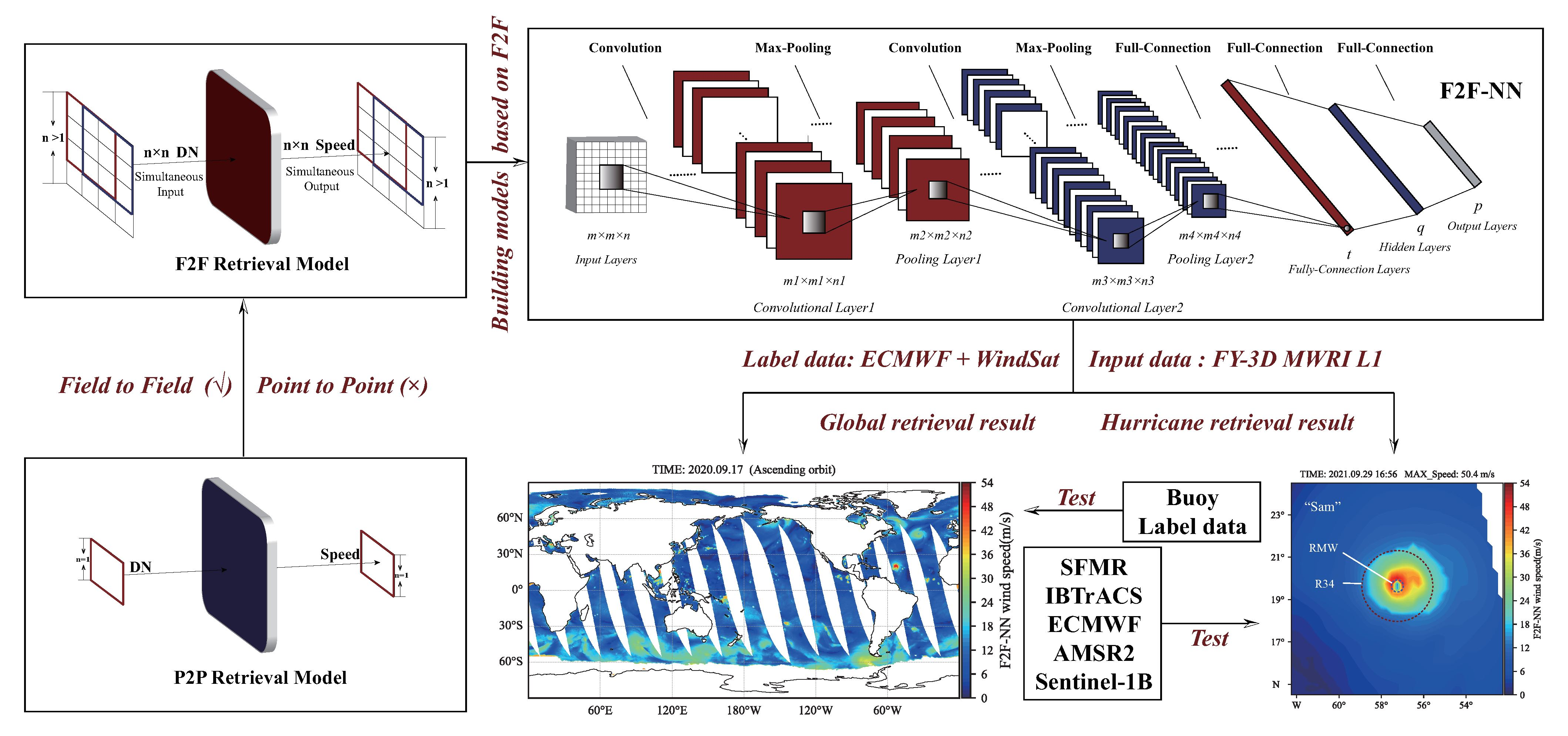
21]. However, the information of adjacent wind vector cells in the true wind field changes continuously; that is, the wind field has continuous characteristics in geographic space. If the continuous feature is applied to SSWS retrieval, the accuracy and authenticity of the retrieval results can theoretically be improved. Since the P2P method does not consider the continuity between adjacent wind vector cells, the consistency of the retrieved wind field is poor. In order to solve the above problems, we propose the retrieval method named F2F. We combine several wind vector cells within a certain range into a continuous wind field, extract the spatial continuity and consistency of the wind field, construct a retrieval model, synchronously retrieve all wind vector cells in the continuous wind field, and finally get more accurate, smooth, and continuous results.
Neural networks have powerful learning, memory, and recognition capabilities [
22] and can explore the complex relationship between wind field observation parameters and wind field information. Back-propagation (BP) neural networks can implement P2P retrieval methods. During the training process, the weights of the BP are continuously modified through error feedback, and finally, the error value tends to be stable. The F2F retrieval method regards the continuous wind field composed of multiple wind vector cells as an image. If the BP neural network is used to process image data, the number of input nodes is the product of the number of pixels and the number of parameters, which adds a huge amount of computation. In addition, an important process of image processing is to capture the feature information between image pixels, and the ability of the BP neural network in this respect is not enough. Moreover, the nonlinear relationship of wind field information is very complex, and the more layers of the neural network, the more favorable it is to express deeper feature information. However, the number of layers of the BP neural network should not be designed too deep because the gradient transmission of the network can hardly exceed 3 layers. Therefore, the BP neural network is not suitable for processing image data and is not suitable for the F2F method. In order to better process image data, a more advanced neural network suitable for image processing is constructed, namely a CNN [
23]. Through weight sharing, the CNN reduces the connection between layers and reduces the risk of overfitting [
24]. Setting the pooling layers in the CNN further reduces the number of parameters, greatly simplifies the complexity of the model, and improves the robustness. Therefore, we construct a wind speed retrieval method based on the basic framework of CNN to accurately mine image data features and accurately describe the mathematical relationship between observation parameters and wind field information. The retrieval model runs faster, and the retrieval work is more efficient.
To sum up, we propose a method for retrieving SSWS from FY-3D MWRI data based on the basic framework of a CNN. Fully considering the spatial consistency of the wind field and the continuity between the wind fields, with the excellent image processing capability of a CNN, the SSWS can be efficiently retrieved, and more accurate, smooth, and continuous sea surface wind fields can be obtained. The background introduction and method are mentioned in
Section 1. The dataset used in this paper is detailed and preprocessed in
Section 2.
Section 3 introduces the main retrieval method proposed in this paper. Comparing the retrieval results and other wind products, we validate and test the retrieval accuracy of F2F-NN in
Section 4. Finally, the work is discussed and summarized in the last two sections [
2].
2. Data
2.1. Microwave Radiometer Wind Field Data
2.1.1. FY-3D MWRI
FY-3D MWRI has five frequency points in the 10.65 - 89 GHz frequency band, each frequency point includes vertical and horizontal polarization modes, a total of 10 channels [
25]. The 89 GHz channel is very sensitive to precipitation scattering signals and is mainly used to obtain surface precipitation information. However, the observation of the sea surface wind field is often greatly affected by precipitation and clouds, so the 89 GHz band data is not used in sea surface wind field retrieval. Low channels can penetrate clouds, rain, and the atmosphere and are sensitive to surface roughness and dielectric constant. It is mainly used for all-weather collection of geophysical parameters such as global sea ice, sea surface temperature, wind speed, and soil moisture. In this paper, we select the information of eight channels other than 89 GHz to retrieve SSWS.
The FY-3D MWRI products are mainly L1 track data (FML) and SWS track wind speed data (FMS). The FML data mainly include scientific data, such as calibration, positioning, and quality information generated by preprocessing of microwave imager, which is used to generate global atmospheric products, sea surface products, and surface products. The
in FML data stores the brightness temperature of each channel after track calibration. In order to save storage space, FML format conversion is performed. The brightness temperature value can be calculated by Equation (
1), and the unit is K. The FMS data are the wind speed product generated corresponding to the FML data, which covers the global sea surface with a spatial resolution of 0.25°. The FMS is generated by a multi-channel regression method and can be used to characterize SSWS.
where
is the brightness temperature, and
is the value stored in
.
2.1.2. WindSat Polarimetric Radiometer (WindSat PR)
WindSat PR aims to prove the capability of all polarization radiometers to measure sea surface wind field, which is developed by the Remote Sensing Department (RSS) of the U.S. Naval Research Laboratory (NRL), the U.S. Naval Space Technology Center, and the National Polar Orbiting Environmental Satellite System (NPOESS). WindSat PR is well calibrated and operates in five discrete channels: 6.8, 10.7, 18.7, 23.8, and 37.0 GHz. The wind speed data of WindSat PR has strong integrity, and its accuracy is also widely recognized [
26].
2.1.3. Advanced EOS Microwave Scanning Radiometer 2 (AMSR2)
AMSR2 was launched from the Tanegashima Space Center on 18 May 2012 to continue the AMSR-E observation mission. The AMSR2 mirror diameter was increased from 1.6 to 2 m, effectively improving the spatial resolution. AMSR2 covers a width of 1450 km of the earth’s surface in one scan, and the observations obtained in two days can cover more than 99% of the world. The detector has the advantages of high resolution, high precision, suitable observation scale, etc. The SSWS products formed by AMSR2 have high precision and reliability [
27].
2.1.4. HY-2B Scanning Microwave Radiometer (HY-2B SMR)
The high accuracy of SSWS data produced by the HY-2B SMR has been verified by the research of scholars [
28]. We introduce the L2 wind speed data to test the accuracy of other similar products in this paper. The L2D data of the L2 product is standard grid SSWS data with a spatial resolution of 0.25°, where
stores global SSWS data.
2.2. Buoy Data (NDBC and TAO)
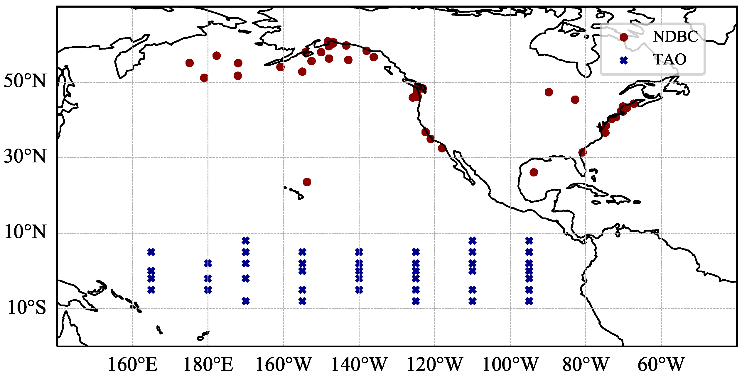
Although the number of buoys is small and the distribution is scattered, the observed wind speed data is the closest to the true wind field, which is of great significance for verifying the accuracy of the satellite’s wind products. We select 41 TAO buoys in the Central Pacific and 41 NDBC buoys near North America in this paper. The surface wind observations with a temporal resolution of 10 min at the height of 4 or 5 m are selected as the validation data for this experiment, and the buoys’ locations are shown in
Figure 1.
2.3. Other Relevant Data
2.3.1. European Centre for Medium-Range Weather Forecasts (ECMWF) ERA5
ECMWF ERA5 is the fifth generation of ECMWF-reanalysis data of global climate and weather in the past 40 to 70 years. It covers the global sea surface, with a spatial resolution of 0.25° and a temporal resolution of up to 1 h, and it is updated daily. ECMWF ERA5, which combines a meteorological model and observation data, is the most accurate global SSWS data under the condition of medium and low wind speeds [
2].
2.3.2. Synthetic Aperture Radar (Sentinel-1)
The Sentinel-1 satellite is part of the European Space Agency (ESA) and the European Commission Copernicus program; this series of satellites is for environmental monitoring. The Sentinel-1 series of satellites consists of two satellites, the Sentinel-1A (S1A) satellite and the Sentinel-1B (S1B) satellite, which operate in the same orbital plane. The Sentinel-1 satellite is equipped with C-band imaging instruments for reliable large-scale observation work. The Sentinel-1 satellite images the world’s land, coasts, and shipping routes with high resolution. This ensures the ability to perform programming tasks and facilitates the construction of long time-series datasets. In this paper, we select the sea surface wind speed product of the Extra Wide (EW) swath mode of the Sentinel-1B satellite to test the accuracy of the retrieval results.
2.3.3. Stepped-Frequency Microwave Radiometer (SFMR)
During the Atlantic and Eastern Pacific hurricane seasons, the National Oceanic and Atmospheric Administration (NOAA) will use aircraft to pass through the center of the storm and use equipment such as the airborne Stepped-Frequency Microwave Radiometer (SFMR) to observe tropical cyclones. Scholars’ studies [
29] show that airborne SFMR observations play an important role in typhoon research, and SFMR wind speed observations also provide important data reference and retrieval basis for some satellite sensors. In this paper, we use SFMR wind speed observations along the aircraft trajectory to test the wind speed accuracy of the retrieval results. In order to minimize the influence of the typhoon wind speed over time on the research, we only select the SFMR wind speed within 1 h of the satellite observation time for analysis and the SFMR observation wind speed with a time interval of more than 1 h is not discussed.
2.3.4. International Best Track Archive for Climate Stewardship (IBTrACS)
IBTrACS is the most complete collection of tropical cyclones in the world and is used by many studies as true hurricane wind data. It combines recent and historical tropical cyclone data from multiple agencies into a unified, open, and best-in-class tracking dataset, resulting in improved inter-agency comparisons [
30].
2.4. Data Preprocessing
The data mentioned above are organized in different ways, so we need to match and unify many different data to complete the experiment.
2.4.1. Time Match
In order to maintain the accuracy of the radiometer data as much as possible, we use the three-node interpolation method to interpolate other corresponding data based on the observation time of the radiometer. Assuming that the three closest moments (if the time of the data is more than 6 h from the moment to be interpolated, we discard the data) to the FML observation time
t in other data are
,
, and
, respectively, and the corresponding wind speed values are
,
, and
. According to Equations (2) and (3), the wind speed value
v at the moment of
t is obtained, where
<
<
t <
and
is a temporary value.
2.4.2. Location Match
We spatially match the different data involved in the experiment, interpolating irregularly arranged data sampling points on a standard grid. We design an inverse distance weighted interpolation method based on a fixed number of interpolation points. We calculate the distance from the interpolation point to each irregularly arranged point and filter the
m data points closest to the interpolation point. Data points outside the resolution grid (that is, the spatial resolution of the training and validation data used in this paper, the same as 0.25° × 0.25°) are removed, and the remaining
n data points are interpolated using the Inverse Distance Weighting (IDW) method (shown in Equation (
4) and (5)),
where
is the distance between each interpolation point and the interpolation center,
is the interpolation result,
and
are the location coordinates of the interpolation center,
and
are the location coordinates of each data point participating in the interpolation,
is the value of each data point participating in the interpolation,
p is the power of distance, which significantly affects the result of interpolation, and its selection criterion is the minimum mean absolute error, the higher the
p, the smoother the interpolation result, and
p = 2 is often chosen [
31].
2.4.3. Height Match and Time Averaging Match of Wind Field
The wind heights of the various wind products mentioned above vary. The sea surface wind height analyzed in this paper is 10 m, and we need to unify the wind field data at other heights to a height of 10 m according to Equation (
6) [
32]. In addition, in IBTrACS data, the U.S. agencies (NOAA and JTWC) report a 1 min averaging time for the sustained (i.e., relatively long-lasting) winds. In most of the rest of the world, a 10 min averaging time is used for "sustained wind" (same as our paper). It is possible to convert from peak 10 min wind to peak 1 min wind (roughly 12% higher for the latter) as a general rule.
where
h represents the height of the wind field, and
and
represent the wind speed at 10 m and
H m heights, respectively.
3. Methodology
3.1. F2F-NN
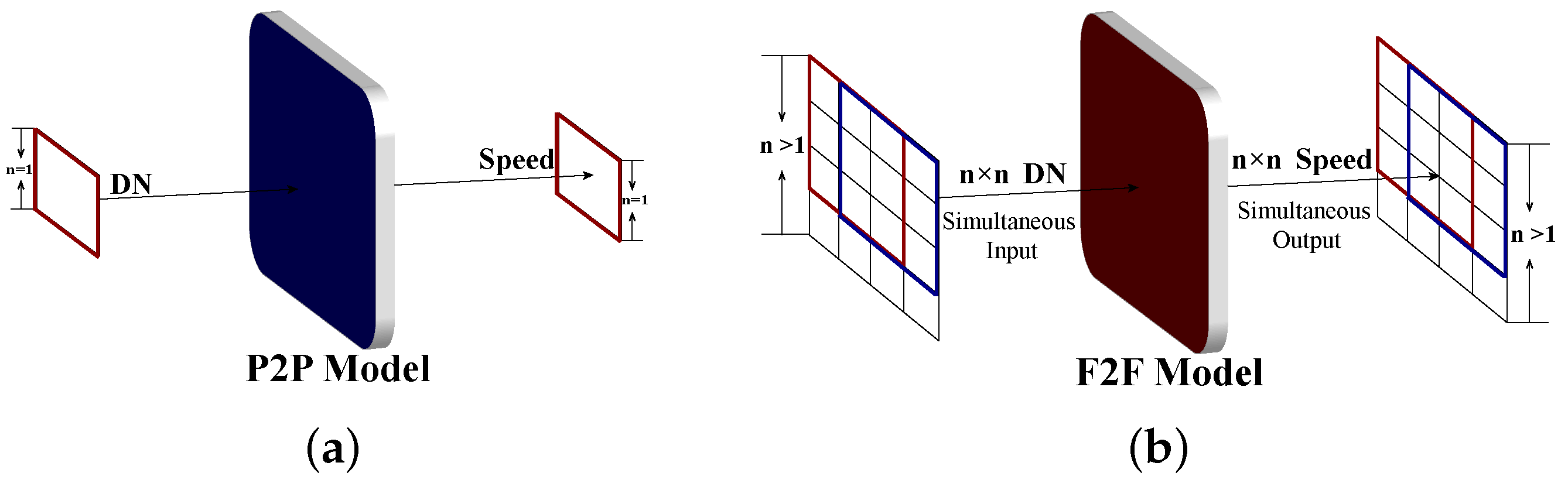
The P2P method (
Figure 2a) is to input the satellite observation data of a single sampling point (
n = 1) into the retrieval model and retrieve the wind speed of the sampling point. This process is repeated until the retrieval of all wind vector cells is completed. We propose the F2F method to solve the problem that the P2P method does not consider the spatial continuity between adjacent wind fields, which can maintain the continuity of the wind field and obtain products that are closer to the true wind field. The F2F method combines multiple adjacent wind vector cells into a continuous wind field of size
n ×
n (the red and blue 3 × 3 boxes in
Figure 2b each represent an
n ×
n continuous wind field), and adjacent multiple
n ×
n continuous wind fields partially overlap. Extract the spatial consistency of a single
n ×
n wind field and the continuity between adjacent
n ×
n wind fields, apply them to the retrieval process and simultaneously obtain the retrieval results of all wind vector cells in the
n ×
n wind field.
It is a very important task to explore the wind field size that is most suitable for the retrieval model. Generally, the larger the wind field, the more information it covers, and the higher the retrieval accuracy is. However, as the area of the wind field increases, the computational cost also increases. When the wind field area increases to a certain value, the improvement of the wind field accuracy does not change significantly, and the increased computational cost is much higher than the benefit brought by the improved retrieval accuracy. According to Vladimir M. Krasnopolsky’s research, when the side length
n of the wind field reaches 8–10, the retrieval accuracy and calculation cost are within the ideal range [
21]. Through pre-experiments, we test the accuracy of the wind field when the side length of the wind field is 7–11. The results show that when
n = 9, the retrieval accuracy is the best, and the performance of the existing computing hardware can meet the computational complexity (computational cost) under this case. Therefore, the side length of the continuous wind field is set to 9 in this paper.
CNNs are widely recognized for their excellent image processing capability [
33]. Based on the basic framework of a CNN, the F2F method is used to design and build a neural network retrieval model to efficiently obtain more accurate, smoother, and more continuous wind field results. We name this retrieval method F2F-NN.
3.2. Construction of F2F-NN Model
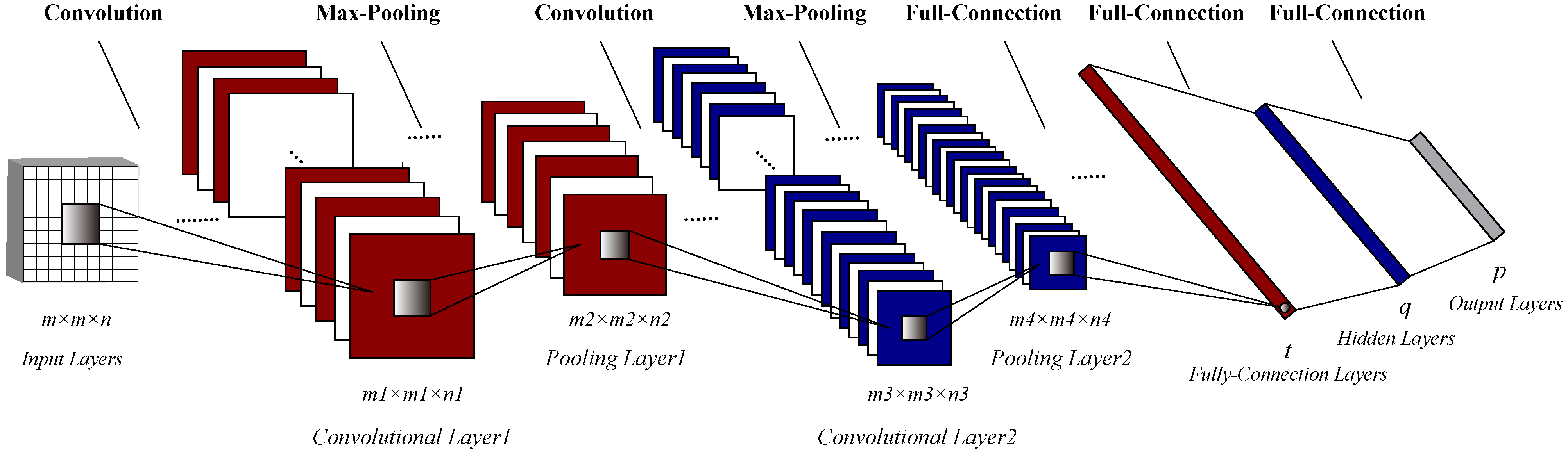
The 8 channels of data of the low frequency of FY-3D MWRI are used in this experiment, so the size of the input wind field is 9 × 9 × 8. We design the first convolutional layer to extract continuous features within an n×n wind field. is set to 1; setting a small convolution kernel (size 3 × 3, number 100) is more conducive to preserving detailed information. is set to , keeping the output size of this layer unchanged, which is beneficial to preserve the edge information in the field. After the first convolutional layer, we set the first max-pooling layer, is set to 1, and the size of the filter is set to 2 × 2. The max-pooling layer has feature invariance and can eliminate outliers. We set the second convolutional layer (the size of the convolution kernel is 3 × 3, the number of convolution kernels is 70, and is the same as the first layer), which not only further extracts the spatial consistency features in the n × n wind field, and also extract the continuity features of the overlapping parts between adjacent n × n wind fields. After the second convolutional layer, we set up a max-pooling layer. is set to 2, and the filter size is set to 2 × 2, which can reduce the size of the data space and the amount of calculation and also control over-fitting to a certain extent.
Essentially, the convolutional layers provide a meaningful, low-dimensional and almost constant feature space. By setting the fully connected layers, highly abstract features after many convolutions can be integrated, and these nonlinear combination features can be simply learned. We expand the feature maps of the second max-pooling layer to get a fully connected layer with 4 × 4 × 70 nodes. We set the number of nodes in the hidden layer to 560 and finally set the number of nodes in the output layer to 81, corresponding to 81 wind vector cells in the 9 × 9 wind field. The structure of the F2F-NN is shown in
Figure 3, and the specific settings of the network are detailed in
Table 1.
Other model parameters are set as follows, is set to 64, is set to 200, and is the same as , which is the most important index for evaluating the retrieval accuracy. of all layers is set to the function, which is simple in calculation and easy to optimize. The chooses , which comes from adaptive moment estimation and is also a variant of the gradient descent algorithm. If the is too large, the parameters to be optimized fluctuate around the minimum value and do not converge; if the is too small, the parameters to be optimized converge slowly. Therefore, we set the to 0.001.
3.3. Selection of Experimental Data
The F2F-NN method requires input data, label data, train data, test data, and other validation data. We select FML data from 19 September 2018 to 19 September 2019 for the train data of the F2F-NN. It is also necessary to construct a label dataset corresponding to the input data in order to complete the training of the network. According to the study by Portabella M et al. [
34], the ECMWF wind speed is compared with MARS buoy’s wind speed, and the results show that when the wind speed exceeded 17 m/s, the ECMWF data significantly underestimated the measured wind speed under strong wind conditions. Therefore, we select ECMWF wind speed data as the label data for wind fields below 17 m/s [
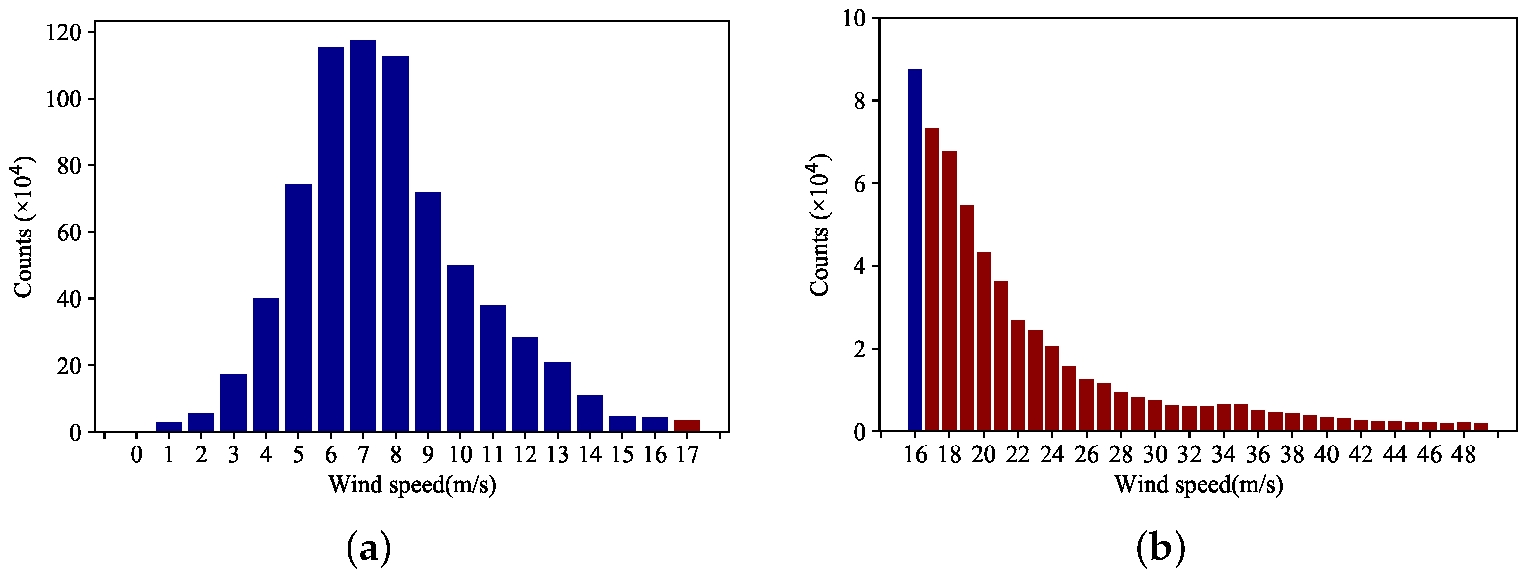
35]. In addition, WindSat data has been proven to have high accuracy and strong data integrity at medium and high wind speeds, so we use WindSat wind speed data as the label data for wind fields over 17 m/s. The wind speed distribution of the training data is shown in
Figure 4a,b. The wind speed of the dataset is mainly concentrated in 5–15 m/s.
To test the generalization ability of the F2F-NN, we construct two test datasets [
36]. The first test dataset consists of FML from 17 September to 17 October 2020. We select the data from one year after the observation time of the training data for verification and use the data from one whole month to fully prove the generalization ability of F2F-NN. The overall retrieval accuracy of the model is tested using the corresponding label data, and the retrieval results are further verified using the buoy wind speed. The second test dataset is the data of Hurricane
(14.5°N–24.5°N, 52°W–62°W), which occurred at 16:56 on 29 September 2021. The time of the second test dataset is two years after the observation time of the training data, and the time interval is large enough to analyze the retrieval ability of F2F-NN. We use reanalysis, radiometer, SAR, SFMR, and hurricane best path data to analyze the retrieval results of complex high-speed wind fields.
3.4. Accuracy Evaluation Index
In order to fully describe the accuracy of the wind speed retrieval results, we select four indicators:
,
, correlation coefficient (
r), and scatter index (
).
is the most commonly used and important index to evaluate the accuracy of wind field retrieval.
can be a good representation of the overall deviation of the predicted data from the label data. The correlation coefficient (
r) can evaluate the linear correlation between the data and reflect the fitting reliability of the neural network. In addition,
can evaluate the fit ability of the retrieval model. The calculation equations of these four indicators are as follows:
where
and
respectively represent the two data sets participating in the test,
and
are the averages of
and
, respectively, and
n represents the amount of data.
4. Results Analysis
The input data processed by the Z-score normalization method have a mean of 0 and a standard deviation of 1. After 100 iterations, the F2F-NN drops significantly. After 200 iterations, () stabilizes at about 0.25 m/s. After many adjustments, the F2F-NN SSWS retrieval model is finally obtained.
4.1. Wind Speed Validation Using Label Data for the First Test Dataset
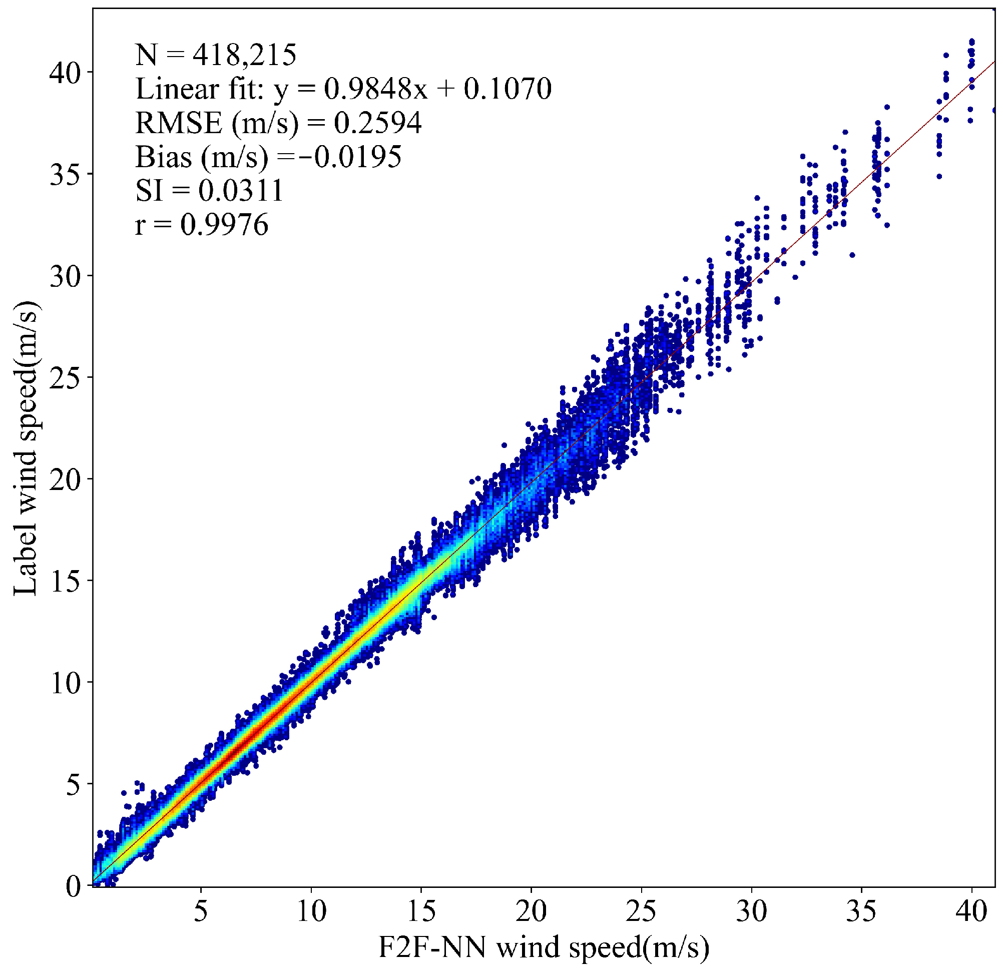
There are a total of 418,215 (
N) data in the first test dataset.
Figure 5 shows that the
of the wind speed is 0.2594 m/s, the
is −0.0195 m/s, the retrieval results are very close to the label data, and the F2F-NN model does not have systematic errors. The
r and
are 0.9976 and 0.0311, respectively, which also shows that the F2F-NN model has a strong generalization ability and a good fitting effect in different wind speed intervals. When the wind speed is higher than 25 m/s, the error increases gradually; this is because the data of high-speed wind is less, and the model training in this interval is not sufficient.
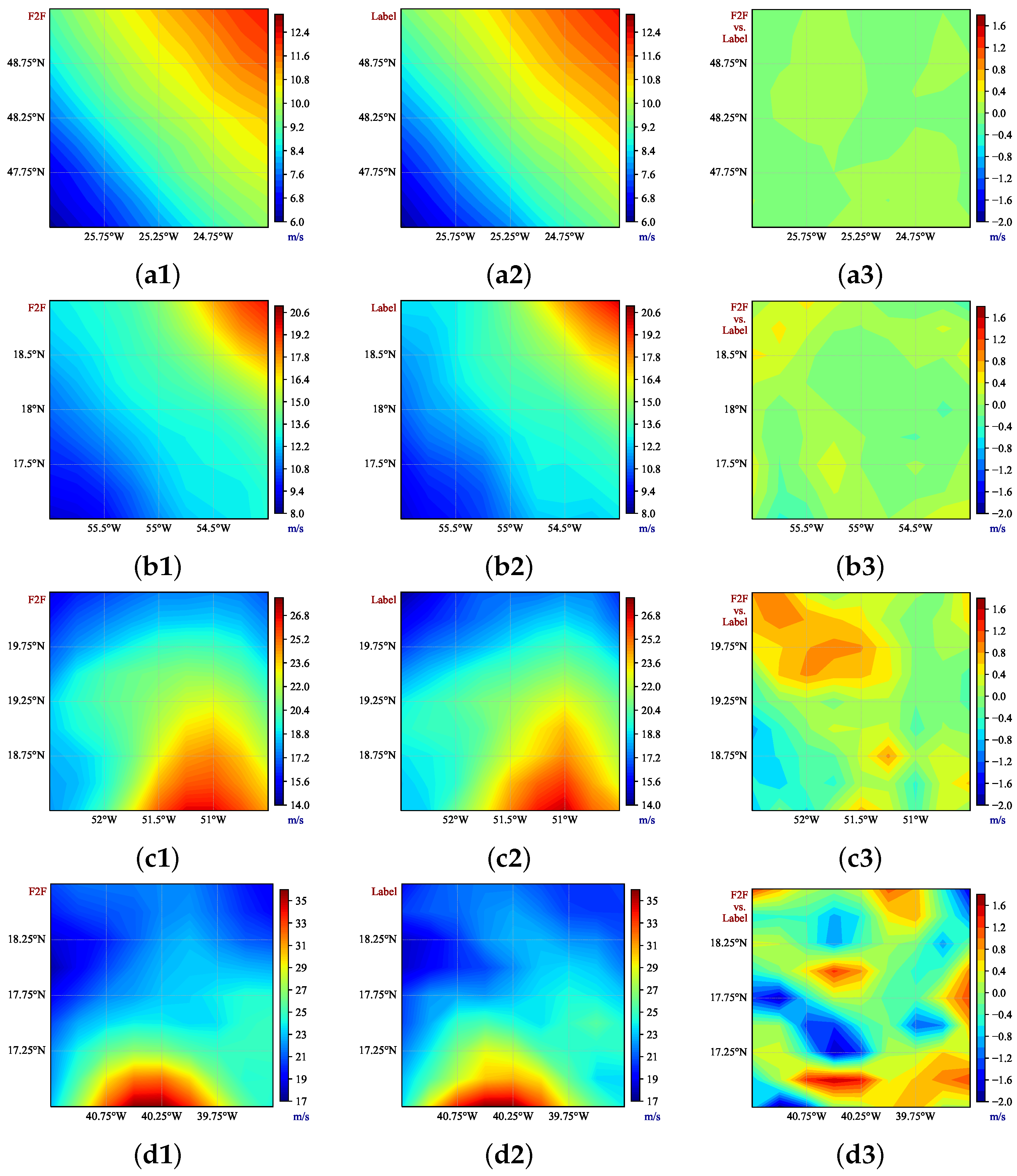
To further analyze the retrieval ability of the F2F-NN model, we visualize the retrieved wind field, label wind fields, and their differences. The input data size of the neural network is 9 × 9, so the visualization is displayed at the same size. It is worth noting that using samples with obvious differences in wind speed within the region is more conducive to analyzing the retrieval ability of the model. Therefore, we select the representative samples of each wind speed interval for analysis.
The wind speed in
Figure 6a is less than 12 m/s, the absolute maximum
between the retrieval result and the label data is less than 0.4 m/s (
Figure 6(a3)), the F2F-NN model has a good fitting result in all parts, and the F2F-NN wind speed changes smoothly and has good continuity. When the wind speed rises to 20 m/s (
Figure 6b), the wind speed distribution of the F2F-NN result is extremely similar to that of the label data, and the absolute
is less than 0.6 m/s (
Figure 6(b3)). When the wind speed rises to 25 m/s (
Figure 6c), the absolute
of the wind speed in the area is still less than 1 m/s, and the F2F-NN wind field is smooth and continuous.
Figure 6d shows part of a hurricane the wind speed exceeds 35 m/s, and the absolute
in the region exceeds 20 m/s (that is, the difference between the maximum wind speed and the minimum wind speed in the area exceeds 20 m/s). F2F-NN has a good fit for each part of the hurricane, and the hurricane structure is clear and accurate. Although the wind speed is underestimated, the absolute
does not exceed 2 m/s; the F2F-NN has an excellent learning effect on label data.
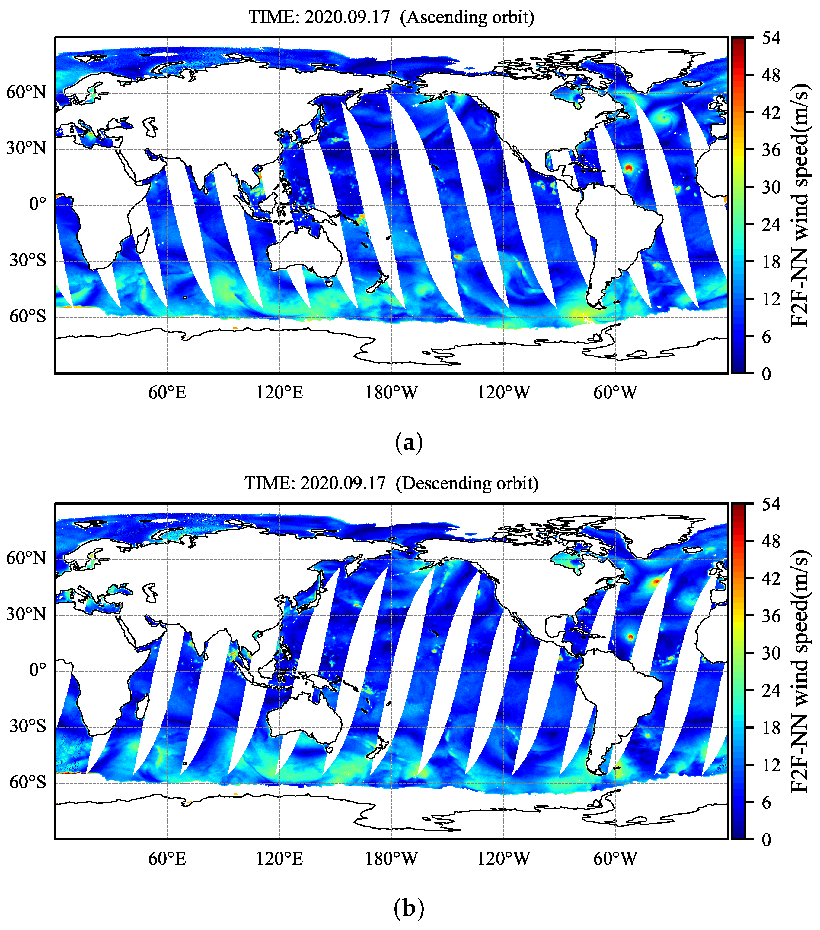
Figure 7 shows the global coverage of the retrieval results of the F2F-NN, from which we can notice possible geographical areas where the retrieval algorithm may struggle. We select the observation data for the whole day on 17 September 2020 in the first test dataset, input it into the F2F-NN model, and display the retrieval results according to the two satellite operating states of ascending and descending orbit.
From
Figure 7a, we can see that the spatial resolution of the F2F-NN retrieved wind field is 0.25°. The areas of land and sea ice (seas near the Antarctic continent and seas near the North Pole) are of no value because in these two areas, the retrieval is useless. In addition, the research goal of our paper is the retrieval of the sea surface wind field, so the sea ice coverage area and the land area are not explored. It is worth noting that, in addition to the above two areas, as long as it is the area scanned by the satellite, we can use the F2F-NN method to retrieve the sea surface wind speed. The F2F-NN method is valid for every region of the globe (where the satellite is observable and its observational data is available). It can be seen from
Figure 7b that the calm wind field in most of the Pacific Ocean and the hurricane wind field in the North Atlantic have been completely retrieved, and the wind field is continuous and smooth.
4.2. Wind Speed Validation Using Buoy Data for the First Test Dataset
The fitting ability of the F2F-NN model to label data has been analyzed above. We introduce the buoy wind speed data to evaluate the true retrieval accuracy of F2F-NN. The wind speed of WindSat, ECMWF, FY-3D, F2F-NN, and HY-2B wind products are tested for accuracy using NDBC and TAO buoy data, respectively, and the test results are shown in
Table 2.
When the NDBC buoy is used for comparison, it can be seen from
Table 2 that the
of F2F-NN wind speed is 0.9097 m/s (the smallest) and has higher accuracy than that of FY-3D (1.4859 m/s), and the goal of improving the accuracy proposed by F2F-NN in design is achieved. The
r of F2F-NN data is the closest to 1 (0.9213), and the
is 0.0520, which indicates the overall difference between F2F-NN wind speed data and NDBC buoy is the smallest. In addition, the HY-2B SMR data also has excellent accuracy but cannot be used as label data due to serious data missing.
When the TAO buoy is used for comparison, the
s of the five wind fields are all lower than their
s when tested with the NDBC buoy. The TAO buoys are distributed near the equator, where the geostrophic deflection force is small, and it is difficult to form high-speed wind in this area [
37]. Due to the simple structure of the wind field and the low retrieval difficulty, the
in this area is low. It can be seen from
Table 2 that the F2F-NN has the smallest
(0.7312 m/s) and
(0.0864), indicating that the F2F-NN wind field is the most accurate. Although the FY-3D wind field data also has a good performance in accuracy, the F2F-NN model still greatly improves its wind speed accuracy.
4.3. Wind Speed Validation for the Second Test Dataset
As mentioned above, it is the most representative to verify the retrieval ability of F2F-NN by using the wind field with obvious wind speed changes and complex structures. In order to fully analyze the generalization ability of F2F-NN, the time of this dataset is far enough from the collection time of the training data. Therefore, Hurricane , which occurred in the North Atlantic at 16:56 on 29 September 2021, is selected for analysis so as to verify the retrieval ability of the F2F-NN model for a high-speed wind field. Since there is almost no buoy data available in this hurricane area, it is not scientific to use buoy data to test the retrieval accuracy. We select four kinds of wind field data: AMSR2 wind data, reanalysis data (ECMWF), SAR wind data (S1B), and SFMR wind observations to evaluate the overall accuracy of F2F-NN retrieval results. The above data are relatively accurate wind fields in their respective fields, so it is reasonable to use them to test the retrieval accuracy of F2F-NN.
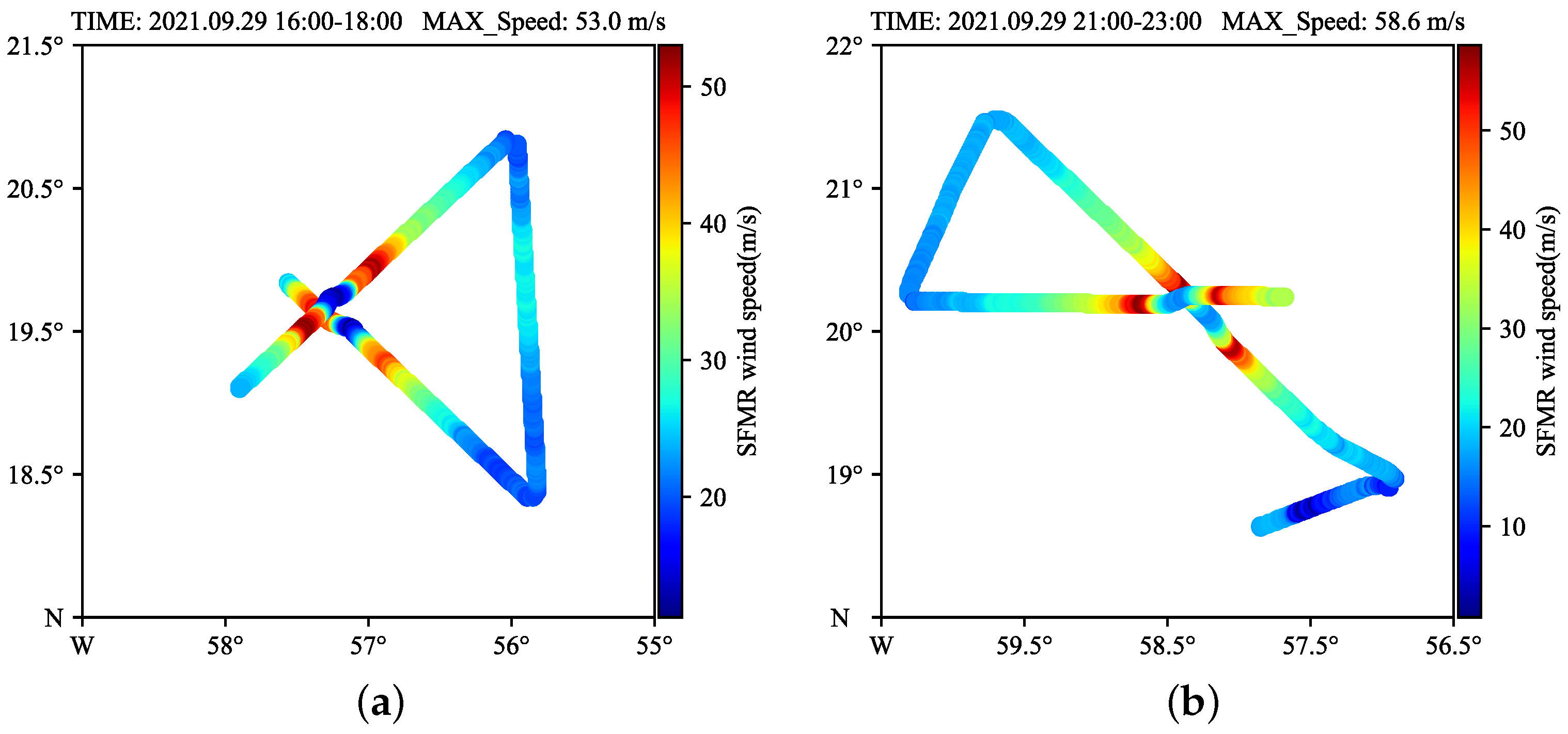
First of all, we use SFMR wind data to test the overall accuracy of various wind products. We match the SFMR data with various wind field data, and the time difference between the matched SFMR and other wind field data is no more than 1 h (mentioned above). The SFMR data we selected are shown in
Figure 8, where the data in
Figure 8a are used to test AMSR2, ECMWF, F2F-NN, and FY-3D wind field data, and the data in
Figure 8b are used to test S1B.
It can be seen from
Table 3 that compared with SFMR wind speed products, the
and
of F2F-NN are at the forefront, much smaller than those of AMSR2, ECMWF and FY-3D, and almost the same as those of S1B (2.2633 m/s). The
r of F2F-NN is the highest (0.9592), indicating that the consistency between the F2F-NN and SFMR data is excellent. In addition, the
performance of F2F-NN is much better than that of S1B, and the overall
of F2F-NN and SMFR is the smallest. It is worth noting that the performance of AMSR2 is also good; the
and
r of AMSR2 are similar to those of F2F-NN. However, FY-3D and ECMWF performed poorly, and both products greatly underestimated the wind speed in the wind field. In conclusion, the performance of F2F-NN is significantly ahead of FY-3D, and F2F-NN has good overall retrieval accuracy for high-speed wind fields.
The F2F-NN wind field is retrieved based on the L1 data of FY-3D, so it is necessary to compare the F2F-NN wind with the FY-3D wind product. The data have been compared with SFMR data above, and the results show that the F2F-NN wind field is dominant in all aspects. However, SFMR data is sparse, so it is more convincing to select more comprehensive data to test the accuracy of F2F-NN. S1B data has a high spatial resolution, and AMSR2 has good high-speed wind observation ability, so we choose AMSR2 and S1B wind field data with good accuracy (shown by comparison with SFMR) to further test the accuracy of the F2F-NN data and FY-3D products.
Table 4 shows that F2F-NN outperforms FY-3D in various metrics, whether compared with AMSR2 or S1B. The FY-3D data underestimates the overall wind speed of the wind field (
< 0), and the
of the F2F-NN is much lower than that of the FY-3D.
It has been proven that the overall retrieval accuracy of the F2F-NN model for high-speed wind fields is excellent. Next, we specifically analyze the wind structure of Hurricane
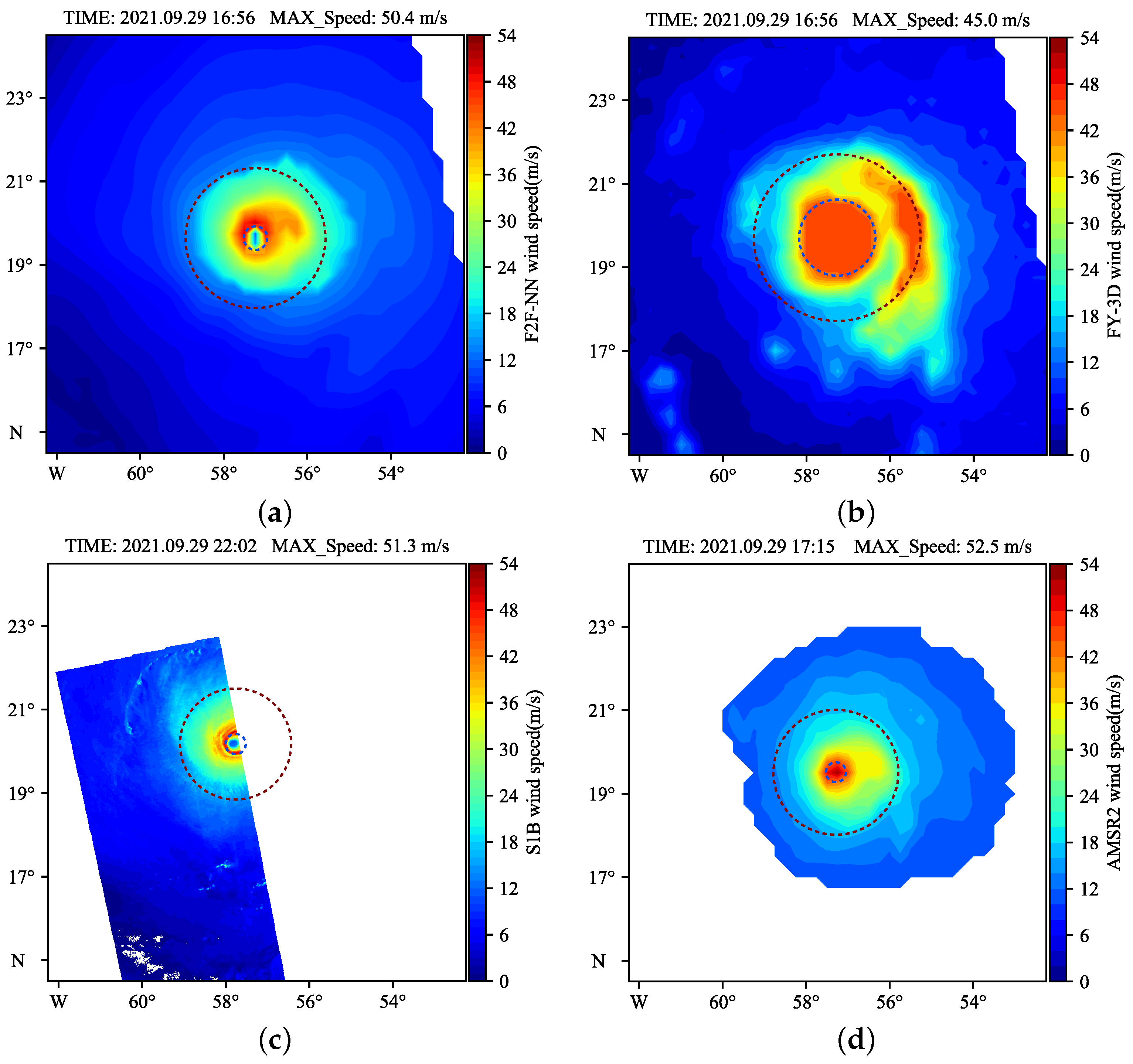
and further illustrate the performance of the F2F-NN model in maintaining the continuity and consistency of wind field structure. Visualize four hurricane wind field products and intuitively analyze the characteristics of hurricane wind fields. In the wind field of F2F-NN (
Figure 9a), compared with S1B and AMSR2, the F2F-NN data are more complete (AMSR and S1B data are largely missing), and they have a complete description of the entire hurricane area (the hurricane eye, high wind area, and edge area are clear). The F2F-NN wind speed changes continuously, and the wind field is smooth and consistent. The FY-3D wind field (
Figure 9b) is saturated with wind, the maximum wind speed can only reach 45 m/s, and it cannot show the complete structure of the hurricane eye and the high wind area. AMSR2 (
Figure 9d) also cannot show the hurricane eye structure. S1B (
Figure 9c) can clearly display the hurricane eye, and because of its high spatial resolution, it can display more complete details of the wind field.
The IBTrACS data are used to analyze the detailed indicators of Hurricane
, the RMW represents the radius of maximum wind speed (an important indicator to describe the structure of the hurricane), the MAX Speed represents the maximum wind speed of the hurricane (hurricane strength) and R34 Mean represents the mean of 34 knots (17.49 m/s) of the wind radii maximum extent in four quadrants. In
Figure 9, the dark red dashed circles represent R34 Mean, and dark blue dashed circles represent RMW.
IBTrACS data shows that the MAX Speed of Hurricane
is 59.2 m/s (true value) at 17:00, and the hurricane wind fields in
Table 5 all underestimate the MAX Speed of the hurricane. The MAX Speed of F2F-NN and AMSR2 differs very little from the IBTrACS data (
< 9 m/s). It is worth mentioning that the maximum wind speed of ECMWF is very different from the true value, even reaching 32.2 m/s, which proves that the reanalysis data is not suitable for describing high-speed wind. This is why we chose WindSat data instead of ECMWF data as the wind speed label value for high-speed wind field.
The S1B and AMSR2 data perform very well on the RMW metric ( < 2 km). The RMW of F2F-NN is 31.04 km, which is only 3.26 km from the RMW of IBTrACS (27.78 km). F2F-NN is very accurate in describing the regional structure near the hurricane center. In addition, reanalysis data generally amplifies the RMW, while radiometer and SAR data degrade the RMW. The analysis is not meaningful in FY-3D data due to wind saturation.
The difference between the R34 Mean of the F2F-NN data and the true value (163.21 km) is 20.98 km, and the 34-knot wind speed distribution range is very close to the true wind field. The performance of AMSR2 is the best, which further illustrates the feasibility of using AMSR2 data to perform the overall accuracy test of the F2F-NN wind field in the previous paper. The R34 Mean of FY-3D is much larger than the true value.
To sum up, the F2F-NN wind field performs well in all evaluation metrics and has a complete wind field structure and obvious continuity characteristics. In addition, the F2F-NN has a strong ability to retrieve high-speed wind fields.
5. Discussion
In recent years, the retrieval of SSWS based on satellite data has become a hot research topic. Improving the retrieval accuracy and maintaining the original characteristics of the wind field are the keys to accurately obtaining SSWS information, especially for the retrieval of high-speed wind fields. As a passive remote sensing device, the low-frequency channel of the microwave radiometer has a strong ability to penetrate clouds and rainfall areas, which can respond well to high-speed wind fields in extreme weather. Therefore, it is very advantageous to use radiometer observation data to retrieve the high-speed wind fields.
The retrieval method based on the physical mechanism clearly describes the physical process of the retrieval, but the complexity of the model is high, which leads to high computational costs. The statistical retrieval method is simple and efficient, but it has the defects that the description of the physical process is not obvious, and the retrieval accuracy of the special scenes is not ideal. The proposed neural network method provides a new idea for the retrieval of SSWS. Theoretically, on the premise of sufficient training data, the neural network can approximate any relational function with its strong learning ability and nonlinear approximation ability. However, the conventional BP neural network has insufficient learning ability for complex retrieval mechanism, and image processing ability, which can only satisfy the P2P retrieval method. Moreover, the P2P method does not consider the spatial continuity characteristics of the wind field, so the retrieval results are often not smooth enough and not close enough to the true wind field. Therefore, we design a stronger network in this paper to accurately retrieve the wind field.
Efficient processing, accurate results, and closer approximation to the true wind field structure are the main goals of the retrieval work. Conventional retrieval methods have problems such as a too complex retrieval model, insufficient data utilization, low retrieval result accuracy, and discontinuous wind field. To solve the problems in conventional retrieval methods, we propose a F2F SSWS retrieval method (F2F-NN) based on a CNN and apply it to wind field retrieval from radiometer data. F2F-NN fully considers the spatial correlation and continuity between adjacent sea surface wind fields and inputs the observation data of continuous wind fields within a certain range into the constructed neural network model so that the SSWS in this range can be obtained synchronously. Compared with physical methods, F2F-NN has lower complexity and better nonlinear relationship fitting ability. Compared with conventional statistical retrieval methods, F2F-NN can adapt to different scenarios with faster operation speed and higher accuracy. Compared with the P2P retrieval method, the retrieval results of F2F-NN are smoother and closer to the true wind field.
As a neural network model, F2F-NN has a strong overall fitting ability to the label data. The model has no systematic errors and is highly correlated with the label data. F2F-NN fully learns the characteristics of the wind field in each region and obtains a continuous and smooth retrieved wind field. We use buoy data to verify the retrieval results, and the accuracy of F2F-NN is superior to many advanced wind field products, especially much higher than that of FY-3D. In addition, F2F-NN has a good retrieval effect on hurricane wind fields, and the results perform well in indicators such as maximum wind speed, RMW, and R34 Mean. In the hurricane field, the characteristics of each part of the wind field are highly similar to the true wind field, and the retrieved wind field has good continuity and integrity. Compared to various radiometer data, reanalysis data, and SFMR data, the accuracy of F2F-NN dominates overall. In addition, the F2F-NN method has a short training time and strong generalization ability, which achieves the expected experimental goals.
The computer CPU used in the experiments is an Intel Core i7-10875H @ 2.30 GHz. Before model training, data preprocessing for a single orbit from FY-3D takes about 4 s. The training dataset contains a total of 10,585 orbits data (29 tracks per day throughout the year), and the total data preprocessing consumes about 11.75 h. During the training process, a single model training is about 5 h. After the retrieval model is obtained, the whole process of retrieval of a single orbital observation data takes about 5 s (including 4 s of data preprocessing, and the retrieval time is less than 0.5 s). The performance of F2F-NN is excellent.
During the process of constructing the F2F-NN model, we explored the impact of the structure of the CNN on retrieval accuracy. Increasing the depth and complexity of neural networks has brought significant improvements in retrieval accuracy while also significantly increasing computational costs. Using the same training data set for training and the computer configuration unchanged, we tested one convolutional layer and one pooling layer. The results show that for each additional convolutional layer and one pooling layer, the running time increases by about 15%, while the model test error decreases by about 4%, and as the depth of the network increases, the growth rate of the running time continues to increase, while the decline rate of the test error continues to decrease. Taking into account the computational time cost and model error, we finally chose a network model consisting of two convolutional layers and two pooling layers. Therefore, comprehensively balancing the calculation cost and retrieval accuracy is the focus of the next work. In addition, it was found that the continuity of the wind field is also reflected in the temporal dimension. The comprehensive utilization of the temporal and spatial continuity of the wind field is expected to further improve the retrieval accuracy of the wind field.
6. Conclusions
Aiming at the retrieval of SSWS, we expect to reduce the difficulty of constructing a complex retrieval model, improve the retrieval accuracy of radiometer wind field (especially high-speed wind field), maintain the spatial continuity of wind field, and obtain retrieval results closer to the true wind field structure.
With the powerful learning ability of the neural network, we construct a network suitable for retrieving SSWS, which greatly simplifies the complexity of the retrieval model and more accurately finds out the mathematical relationship between the observation parameters (brightness temperature) and SSWS. The F2F-NN method can maintain the spatial continuity of the wind field well, and can obtain wind field products that are smoother and closer to the true wind field. We periodically set multiple convolutional layers and max-pooling layers in the F2F-NN model to extract spatial consistency features within n×n wind fields and continuity features between adjacent wind fields. Then, we set small convolution kernels to preserve details and set fully-connection layers to simply learn nonlinear combined features. After many adjustments to the network structure and super-parameters, we finally get the F2F-NN model with excellent retrieval performance. The experimental results are presented in two parts.
The first test dataset is input into the F2F-NN model, and the wind speed retrieval results are obtained. The results show that the F2F-NN method has a strong learning ability for wind field characteristics and an excellent ability to fit the label data. (1) The of wind speed is 0.2594 m/s, and the retrieved wind field is strongly correlated with the label data. F2F-NN has a strong generalization ability and has a good fitting effect on label data. (2) Visually analysis of the response results of F2F-NN in different wind speed intervals. F2F-NN has a good response in different wind speed intervals. In a high-speed wind field, the wind speed change of the retrieved wind field is still stable and continuous, and the wind structure is accurate and clear. (3) The accuracy of WindSat, ECMWF, FY-3D, F2F-NN, and HY-2B is evaluated using buoy data. The retrieved wind field of F2F-NN has obvious advantages in the above five kinds of wind field data. The of F2F-NN is less than 0.91 m/s, which is much better than the accuracy of FY-3D. The F2F-NN method greatly improves the accuracy of the FY-3D product and achieves the desired effect.
The second test dataset is input to the F2F-NN model, and the results show that the F2F-NN method has a strong retrieval capability for high-speed wind fields. (1) Comparing five wind field products with the SFMR data, the overall accuracy of the F2F-NN wind data is the highest, and the of F2F-NN is much lower than that of FY-3D. In addition, the correlation coefficient between the F2F-NN wind field and SFMR data is high, and the wind field similarity is high. The F2F-NN data and FY-3D are tested with high-precision AMSR2 and S1B data, and the F2F-NN data has obvious advantages in all aspects. (2) Comparing the five wind field products with IBTrACS data, the F2F-NN wind field is superior to the other products in terms of maximum wind speed and maximum wind speed radius. The structure of the wind field retrieved by F2F-NN is complete and accurate, and the wind speed changes smoothly and continuously.
To sum up, the F2F-NN retrieval model successfully achieves the desired goal. F2F-NN improves the retrieval accuracy of FY-3D MWRI SSWS data and obtains a smoother and more continuous wind field. In addition, the F2F-NN method also performs well in high-speed wind field retrieval and can accurately and quickly obtain the retrieved wind field, which is close to the true wind field.
Author Contributions
Conceptualization, X.S. and B.D.; Data curation, X.S.; Formal analysis, X.S., B.D. and K.R.; Funding acquisition, K.R.; Investigation, X.S.; Methodology, X.S. and B.D.; Software, X.S.; Supervision, B.D. and K.R.; Validation, X.S.; Visualization, X.S.; Writing—original draft, X.S.; Writing—review and editing, X.S. and B.D. All authors have read and agreed to the published version of the manuscript.
Funding
This work is supported by the National Key R&D Program of China (Grant No. 2018YFB0203801) and the National Natural Science Foundation of China (Grant Nos. 61572510).
Data Availability Statement
Acknowledgments
The authors would like to thank the National Satellite Meteorological Center for providing the FY-3D data, NSOAS for providing the HY-2B L2D data free of charge, the National Centers for Environmental Information for providing the IBTrACS data, the National Data Buoy Center (NDBC) and Tropical Atmosphere Ocean Project (TAO) and the European Center for Medium-Range Weather Forecasts (ECMWF) for providing buoy observations and reanalysis data, Remote Sensing Systems for providing the AMSR2, and WindSat data, and NOAA’s Atlantic Oceanographic and Meteorological Laboratory for providing the SFMR and Sentinel-1 data.
Conflicts of Interest
The authors declare no conflict of interest.
References
- Dou, F.; An, D.; Li, J. Sea Surface Wind Speed Retrieval based on FY-3B Microwave Imager. Remote Sens. Technol. Appl. 2015, 29, 984–992. [Google Scholar]
- Shi, X.; Duan, B.; Ren, K. A More Accurate Field-to-Field Method towards the Wind Retrieval of HY-2B Scatterometer. Remote Sens. 2021, 13, 2419. [Google Scholar] [CrossRef]
- Stuart, K.M.; Long, D.G. Tracking large tabular icebergs using the SeaWinds Ku-band microwave scatterometer. Deep. Sea Res. Part II 2011, 58, 1285–1300. [Google Scholar] [CrossRef]
- Lin, M.; Zou, J.; Xie, X.; Yi, Z. HY-2A microwave scatterometer wind retrieval algorithm. Eng. Sci. 2013, 15, 70–76. [Google Scholar]
- Wang, H. Multi-frequency Dual-polarization Spaceborne Microwave Radiometer Antennas. In Proceedings of the 2020 14th European Conference on Antennas and Propagation (EuCAP), Copenhagen, Denmark, 15–20 March 2020. [Google Scholar]
- McKague, D.S.; Ruf, C.S.; Balasubramaniam, R.; Clarizia, M.P. Validation of High Wind Retrievals from the Cyclone Global Navigation Satellite System (CYGNSS) Mission. In AGU Fall Meeting; NASA/ADS: Cambridge, MA, USA, 2017. [Google Scholar]
- Jiang, Z.H.; Huang, S.X.; Liu, G.; Liu, X.P. Research on the development of surface wind speed retrieval from satellite radar altimeter. Mar. Sci. Bull. 2011, 30, 588–594. [Google Scholar]
- Li, X. Retrieval of Sea Surface Wind Speed from Spaceborne SAR over the Arctic Marginal Ice Zone with a Neural Network. Remote Sens. 2020, 12, 3291. [Google Scholar] [CrossRef]
- Qiang, S.; Daren, L. Analysis on the Performance of Microwave Radiometer on Monitoring Sea Surface Wind under Non-precipitation Conditions. Remote Sens. Technol. Appl. 2016, 31, 109–118. [Google Scholar]
- Tang, F.; Dong, H.; Li, N.; Liu, C. Geolocation errors and correction of FY-3B microwave radiation imager measurements. J. Remote Sens. 2016, 20, 1342–1351. [Google Scholar]
- Zou, X. Studies of FY-3 Observations over the Past 10 Years: A Review. Remote Sens. 2021, 13, 673. [Google Scholar] [CrossRef]
- Yang, J.; Jiang, L.; Wu, S.; Wang, G.; Liu, X. Development of a Snow Depth Estimation Algorithm over China for the FY-3D/MWRI. Remote Sens. 2019, 11, 977. [Google Scholar] [CrossRef] [Green Version]
- Hao, G.; Xu, R.; Wu, S. Accuracy Evaluation of the FengYun-3C Global Land Surface Temperature Products Retrieval from Microwave Radiation Imager. Meteorol. Environ. Sci. 2018, 41, 1–8. [Google Scholar]
- Rui, W.; Shi, S.W.; Yan, W.; Wen, L. Sea surface wind retrieval from polarimetric microwave radiometer in typhoon area. Chin. J. Geophys. 2014, 57, 738–751. [Google Scholar]
- Goodberlet, M.A.; Swift, C.T. Improved retrievals from the DMSP wind speed algorithm under adverse weather conditions. IEEE Trans. Geosci. Remote Sens. 1992, 30, 1076–1077. [Google Scholar] [CrossRef]
- Wentz, F.J. AMSR Ocean Algorithm. EORC Bulletin. Tech. Rep. 2002, 9, 8–28. [Google Scholar]
- Wang, Z.; Bao, J.; Yun, L.; Hua, S. Study on retrieval algorithm of ocean parameters for the HY-2 scanning microwave radiometer. Eng. Sci. 2014, 16, 70–82. [Google Scholar]
- Wentz, F.J. A Well-Calibrated Ocean Algorithm for Special Sensor Microwave/Imager. J. Geophys. Res. Ocean. 1997, 102, 8703–8718. [Google Scholar] [CrossRef] [Green Version]
- Wang, Z.Z. A Model for Inversing Sea Surface Wind Speeds by Using SSM/I 19.35 GHz Vertical and Horizontal Brightness Temperatures. Ocean. Technol. 2003, 22, 6–10. [Google Scholar]
- Stogryn, A.P.; Butler, C.T.; Bartolac, T.J. Ocean surface wind retrievals from special sensor microwave imager data with neural networks. J. Geophys.Res. Ocean. 1994, 99, 981. [Google Scholar] [CrossRef]
- Krasnopolsky, V.M. Atmospheric and Oceanic Remote Sensing Applications; Springer: Dordrecht, The Netherlands, 2013; Volume 46, pp. 47–79. [Google Scholar]
- Liu, Z.Y.C.; Chamberlin, A.J.; Tallam, K.; Jones, I.J.; Lamore, L.L.; Bauer, J.; Bresciani, M.; Wolfe, C.M.; Casagrandi, R.; Mari, L.; et al. Deep Learning Segmentation of Satellite Imagery Identifies Aquatic Vegetation Associated with Snail Intermediate Hosts of Schistosomiasis in Senegal, Africa. Remote Sens. 2022, 14, 1345. [Google Scholar] [CrossRef]
- Peng, F.; Lu, W.; Tan, W.; Qi, K.; Zhang, X.; Zhu, Q. Multi-Output Network Combining GNN and CNN for Remote Sensing Scene Classification. Remote Sens. 2022, 14, 1478. [Google Scholar] [CrossRef]
- Gómez-Ríos, A.; Tabik, S.; Luengo, J.; Shihavuddin, A.; Krawczyk, B.; Herrera, F. Towards Highly Accurate Coral Texture Images Classification Using Deep Convolutional Neural Networks and Data Augmentation. Expert Syst. Appl. 2018, 118, 315–328. [Google Scholar] [CrossRef] [Green Version]
- Du, B.; Ji, D.; Shi, J.; Wang, Y.; Letu, H. The Retrieval of Total Precipitable Water over Global Land Based on FY-3D/MWRI Data. Remote Sens. 2020, 12, 1508. [Google Scholar] [CrossRef]
- Gaiser, P.W.; Bettenhausen, M.H.; Li, L.; Twarog, E.M. The WindSat polarimetric radiometer and ocean wind measurements. In Proceedings of the OCEANS, Washington, DC, USA, 17–23 September 2005. [Google Scholar]
- Ricciardulli, L.; Mears, C.; Manaster, A.; Meissner, T. Assessment of CYGNSS Wind Speed Retrievals in Tropical Cyclones. Remote Sens. 2021, 13, 5110. [Google Scholar] [CrossRef]
- Li, Y.; Yin, X.; Wang, S.; Zhou, W.; Ma, C. Extreme High Wind Speed Monitoring with Spatial Resolution Enhancement of HY-2B SMR Brightness Temperature. In Proceedings of the IGARSS 2020—2020 IEEE International Geoscience and Remote Sensing Symposium, Waikoloa, HI, USA, 26 September–2 October 2020. [Google Scholar]
- Fore, A.; Yueh, S.; Tang, W.; Stiles, B.; Hayashi, A. SMAP Tropical Cyclone Size and Intensity Validation. In Proceedings of the IGARSS 2018-2018 IEEE International Geoscience and Remote Sensing Symposium, Valencia, Spain, 22–27 July 2018. [Google Scholar]
- Haakman, K.; Sayol, J.M.; van der Boog, C.G.; Katsman, C.A. Statistical Characterization of the Observed Cold Wake Induced by North Atlantic Hurricanes. Remote Sens. 2019, 11, 2368. [Google Scholar] [CrossRef] [Green Version]
- Kim, S.; Rhee, S.; Kim, T. Digital Surface Model Interpolation Based on 3D Mesh Models. Remote Sens. 2019, 11, 24. [Google Scholar] [CrossRef] [Green Version]
- Wang, H.; Zhu, J.; Lin, M.; Zhang, Y.; Chang, Y. Evaluating Chinese HY-2B HSCAT Ocean Wind Products Using Buoys and Other Scatterometers. IEEE Geosci. Remote Sens. Lett. 2019, 17, 923–927. [Google Scholar] [CrossRef]
- Kussul, N.; Lavreniuk, M.; Skakun, S.; Shelestov, A. Deep Learning Classification of Land Cover and Crop Types Using Remote Sensing Data. IEEE Geosci. Remote Sens. Lett. 2017, 14, 778–782. [Google Scholar] [CrossRef]
- Portabella, M.; Mouche, A.; Polverari, F.; StoffelenKnmi, A.; Zadelhoff, G. CHEFS C-Band High and Extreme-Force Speeds; KNMI and CHEFS Consortium: De Bilt, The Netherlands, 2018. [Google Scholar]
- Marullo, S.; Pitarch, J.; Bellacicco, M.; Sarra, A.; Santoleri, R. Air-Sea Interaction in the Central Mediterranean Sea: Assessment of Reanalysis and Satellite Observations. Remote Sens. 2021, 13, 2188. [Google Scholar] [CrossRef]
- Zheng, Q.; Yang, M.; Yang, J.; Zhang, Q.; Zhang, X. Improvement of Generalization Ability of Deep CNN via Implicit Regularization in Two-stage Training Process. IEEE Access 2018, 6, 15844–15869. [Google Scholar] [CrossRef]
- Ribal, A.; Young, I.R. Calibration and Cross Validation of Global Ocean Wind Speed Based on Scatterometer Observations. J. Atmos. Ocean. Technol. 2020, 37, 279–297. [Google Scholar] [CrossRef]
Figure 1.
Locations of TAO (dark blue) and NDBC (dark red) buoys are used in this paper.
Figure 1.
Locations of TAO (dark blue) and NDBC (dark red) buoys are used in this paper.
Figure 2.
(a) shows the P2P method and (b) is a schematic diagram of F2F.
Figure 2.
(a) shows the P2P method and (b) is a schematic diagram of F2F.
Figure 3.
F2F-NN structure diagram, two convolutional layers and max-pooling layers are arranged periodically and finally connected to the fully connected layers.
Figure 3.
F2F-NN structure diagram, two convolutional layers and max-pooling layers are arranged periodically and finally connected to the fully connected layers.
Figure 4.
The blue histogram indicates that the wind speed is lower than 17 m/s, and the red histogram indicates that the wind speed is higher than 17 m/s. The ordinate ratios of (a,b) are different, and the number of wind fields with a speed higher than 17 m/s is obviously less.
Figure 4.
The blue histogram indicates that the wind speed is lower than 17 m/s, and the red histogram indicates that the wind speed is higher than 17 m/s. The ordinate ratios of (a,b) are different, and the number of wind fields with a speed higher than 17 m/s is obviously less.
Figure 5.
Comparison between F2F-NN wind speed and label wind speed.
Figure 5.
Comparison between F2F-NN wind speed and label wind speed.
Figure 6.
(a1–d1) shows F2F-NN wind fields in different wind speed ranges, (a2–d2) shows label wind fields, and (a3–d3) shows the difference between the F2F-NN wind and label wind.
Figure 6.
(a1–d1) shows F2F-NN wind fields in different wind speed ranges, (a2–d2) shows label wind fields, and (a3–d3) shows the difference between the F2F-NN wind and label wind.
Figure 7.
(a) is the wind field obtained by F2F-NN from the data collected in the ascending orbit of the FY-3D MWRI on 17 September 2020, and (b) is the retrieval result of the descending orbit.
Figure 7.
(a) is the wind field obtained by F2F-NN from the data collected in the ascending orbit of the FY-3D MWRI on 17 September 2020, and (b) is the retrieval result of the descending orbit.
Figure 8.
(a) shows the SFMR data from 16:00 to 18:00, which is similar to the time of the AMSR2, ECMWF, F2F-NN, and FY-3D wind fields. (b) shows the SFMR data from 21:00 to 23:00, which is similar to the time of the S1B wind field.
Figure 8.
(a) shows the SFMR data from 16:00 to 18:00, which is similar to the time of the AMSR2, ECMWF, F2F-NN, and FY-3D wind fields. (b) shows the SFMR data from 21:00 to 23:00, which is similar to the time of the S1B wind field.
Figure 9.
(a–d) are descriptions of Hurricane by F2F-NN, FY-3D, S1B, and AMSR2, respectively.
Figure 9.
(a–d) are descriptions of Hurricane by F2F-NN, FY-3D, S1B, and AMSR2, respectively.
Table 1.
F2F-NN network detailed parameters.
Table 1.
F2F-NN network detailed parameters.
| Feature Maps Size | Layers | Filters | Filter Size | Strides | Padding | Parameters |
|---|
| [9 × 9 × 8] | INPUT | - | - | - | - | m = 9, n = 8 |
| [9 × 9 × 100] | CONV1 | 100 | 3 × 3 | 1 | SAME | m1 = 9, n1 = 100 |
| [8 × 8 × 100] | MAX POOL1 | - | 2× 2 | 1 | VALID | m2 = 8, n2 = 100 |
| [8 × 8 × 70] | CONV2 | 70 | 3 × 3 | 1 | SAME | m3 = 8, n3 = 70 |
| [4 × 4 × 70] | MAX POOL2 | - | 2 × 2 | 2 | VALID | m4 = 4, n4 = 70 |
| [1120] | FC1 | - | - | - | - | t = 4 × 4 × 70 |
| [560] | FC2 | - | - | - | - | q = 560 |
| [81] | OUTPUT | - | - | - | - | p = 81 |
Table 2.
The overall comparison results between various wind products and buoy data.
Table 2.
The overall comparison results between various wind products and buoy data.
| Dataset | NDBC | TAO |
|---|
| RMSE (m/s) | Bias (m/s) | SI | r | RMSE (m/s) | Bias (m/s) | SI | r |
|---|
| WindSat | 1.1568 | 0.1225 | 0.2874 | 0.8836 | 0.9648 | −0.0044 | 0.1145 | 0.8821 |
| ECMWF | 1.0288 | 0.0071 | 0.2571 | 0.9128 | 0.9096 | −0.1044 | 0.1072 | 0.9118 |
| FY-3D | 1.4859 | −0.0204 | 0.3713 | 0.8988 | 1.0743 | 0.0354 | 0.1274 | 0.8137 |
| F2F-NN | 0.9097 | 0.0520 | 0.2269 | 0.9213 | 0.7312 | −0.0676 | 0.0864 | 0.9456 |
| HY-2B | 1.1301 | 0.0153 | 0.2824 | 0.8819 | 0.9105 | 0.0324 | 0.1079 | 0.8745 |
Table 3.
Comparison of SFMR wind data with other wind products.
Table 3.
Comparison of SFMR wind data with other wind products.
| Dataset | AMSR2 | ECMWF | F2F-NN | FY-3D | S1B |
|---|
| (m/s) | 3.4826 | 7.0096 | 2.2980 | 6.3775 | 2.2633 |
| (m/s) | −0.3006 | −5.9849 | −0.2319 | −5.4552 | −1.6166 |
| 0.1258 | 0.1427 | 0.0875 | 0.1130 | 0.0726 |
| r | 0.9247 | 0.9027 | 0.9592 | 0.8865 | 0.8320 |
Table 4.
The overall comparison results of F2F-NN and FY-3D wind speed with other products.
Table 4.
The overall comparison results of F2F-NN and FY-3D wind speed with other products.
| Dataset | AMSR2 | S1B |
|---|
| RMSE (m/s) | Bias (m/s) | SI | r | RMSE (m/s) | Bias (m/s) | SI | r |
|---|
| F2F-NN | 2.0361 | −0.3757 | 0.1795 | 0.9393 | 1.5338 | 0.6045 | 0.2155 | 0.9664 |
| FY-3D | 2.8798 | −1.5485 | 0.2712 | 0.8940 | 2.2467 | −1.1761 | 0.2590 | 0.8574 |
Table 5.
Description results of Hurricane by various wind products.
Table 5.
Description results of Hurricane by various wind products.
| Dataset (Bias) | MAX Speed (m/s) | RMW (km) | R34 Mean (km) |
|---|
| IBTrACS | 59.2 | 27.78 | 163.21 |
| IBTrACS [22:00] | 62.6 | 27.78 | 180.57 |
| AMSR2 | 52.5 (−6.7) | 26.20 (−1.58) | 164.45 (+1.24) |
| ECMWF | 27.0 (−32.2) | 54.94 (+27.16) | 133.29 (−29.92) |
| F2F-NN | 50.4 (−8.8) | 31.04 (+3.26) | 184.19 (+20.98) |
| FY-3D | 45.0 (−14.2) | 100.15 (+72.37) | 219.43 (+56.22) |
| S1B[22:00] | 51.3 (−11.3) | 26.55 (−1.23) | 146.32 (−34.25) |
| Publisher’s Note: MDPI stays neutral with regard to jurisdictional claims in published maps and institutional affiliations. |
© 2022 by the authors. Licensee MDPI, Basel, Switzerland. This article is an open access article distributed under the terms and conditions of the Creative Commons Attribution (CC BY) license (https://creativecommons.org/licenses/by/4.0/).


