Bayesian Estimation of Land Deformation Combining Persistent and Distributed Scatterers

Abstract

Persistent Scatterer Interferometry (PSI) has been widely used for monitoring land deformation in urban areas with millimeter accuracy. In natural terrain, combining persistent scatterers (PSs) and distributed scatterers (DSs) to jointly estimate deformation, such as SqueeSAR, can enhance PSI results for denser and better coverage. However, the phase quality of a large number of DSs is far inferior to that of PSs, which deteriorates the deformation measurement accuracy. To solve the contradiction between measurement accuracy and coverage, a Bayesian estimation method of land deformation combining PSs and DSs is proposed in this paper. First, a two-level network is introduced into the traditional PSI to deal with PSs and DSs. In the first-level network, the Maximum Likelihood Estimation (MLE) of deformation parameters at PSs and high-quality DSs is obtained accurately. In the secondary-level network, the remaining DSs are connected to the nearest PSs or high-quality DSs, and the deformation parameters are estimated by Maximum A Posteriori (MAP) based on Bayesian theory. Due to the poor phase quality of the remaining DSs, MAP can achieve better estimation results than the MLE based on the spatial correlation of the deformation field. Simulation and Sentinel-1A satellite data results verified the feasibility and reliability of the proposed method. Regularized by the spatial deformation field derived from the high-quality PSs and DSs, the proposed method is expected to achieve robust results even in low-coherence areas, such as rural areas, vegetation coverage areas, or deserts.

1. Introduction

Differential Interferometry Synthetic Aperture Radar (DInSAR) is a powerful technique to precisely monitor land deformation, such as seismological activities, volcanism, landslides, and ground subsidence [1,2]. However, it has limitations due to atmospheric artifacts and temporal and geometric decoherence. Under unfavorable conditions, the deformation signal is obscured by atmospheric interference [3], temporal decorrelation noise (introduced by the changes in the scattering characteristics of the target and incoherent movement of individual scattering elements) [4], and geometric decorrelation noise (introduced by changes in radar viewing angles) [5,6].

Persistent Scatterer Interferometry (PSI) technology is an extension of DInSAR techniques that overcomes the limitations of decoherence and atmospheric problems through time-series methods [7,8,9]. PSI technology relies on persistent scatterers (PSs), whose amplitude and phase values are stable over time and imaging geometry [10]. Therefore, such technology has been widely used for monitoring land deformation with millimeter accuracy in urban areas where man-made structures behave like strongly reflecting corner reflectors [11].

However, PSI technology failed to perform satisfactorily in the absence of PSs in non-urban areas [9]. Especially in natural terrain or desert areas, the scattering mechanisms are dominated by distributed scatterers (DSs), whose back-scattered energy is less strong, but shares similar reflectivity values within a wide area. Contrary to PSs, DSs are seriously affected by temporal and spatial decorrelation. Therefore, the observed phases of DSs are much noisier than those of PSs [12]. This makes PSI an opportunistic approach that functionally limits the density of the useful scatterers [13].

Recently, several advanced techniques have been proposed to extract information from DSs and increase the spatial density of measured points. Among them, the most representative techniques are the Small Baseline Subset Algorithm (SBAS) [14] and SqueeSAR [15]. Unlike PSI, the SBAS method relies on multilooked and unwrapped differential interferograms with short spatial and temporal baselines to minimize the effects of decorrelation [16,17,18]. However, the error-prone phase-unwrapping and multi-looking operations in SBAS often lead to poor accuracy and low resolution of the estimated deformation [12]. Moreover, the rectangular multi-looking window in SBAS results in a superposition of different objects on the ground and then a loss of the deformation information contained in the isolated pixels [19]. In addition, the phase unwrapping often results in discontinuous fringes, especially in natural terrains.

In contrast, to reduce the decorrelation noise of DSs, the SqueeSAR method obtains the best possible estimates of the phase history over spatially statistically homogeneous pixels (SHPs) using all possible wrapped interferograms using a phase triangulation algorithm (PTA) [20,21]. The PTA can reduce the stochastic noise in DSs. Then, the DSs and PSs are jointly processed indiscriminately under the traditional PSI processing framework [15,22]. The optimum phase of DSs is estimated from the coherence matrix [23]. Recently, a number of works have recognized that coherence errors due to limited ensembles in data statistics affect the accuracy of InSAR measurements for DSs, especially over low coherence scenarios [24,25,26,27,28]. Moreover, although preprocessing of DSs is often simplistically depicted as transforming DSs into PSs, preprocessed DSs are statistically not equivalent to PSs [29]. In other words, the phase quality of a large number of DSs is far inferior to that of PSs, which deteriorates the deformation measurement accuracy [30,31,32]. In addition, the quality of the estimated phase of DSs can be indicated by the temporal coherence ${\mathsf{\gamma }}_{PTA}$, which can be used effectively for the final selection of DSs with a reliable phase estimation [21,33]. However, a high value of temporal coherence indicates a large agreement between the observations and estimated parameters but fewer DS candidates. A low value of temporal coherence can involve more DS candidates but a large disagreement between the observations and estimated parameters. To sum up, the contradiction between measurement accuracy and coverage has not been fundamentally solved in both SBAS and SqueeSAR.

To solve the contradiction between measurement accuracy and coverage, a Bayesian estimation method of land deformation combining PSs and DSs is proposed in this paper. First, a two-level network is introduced into the traditional PSI to restrain the error propagation of low-quality DSs in the adjustment network. In the first-level network, the deformation parameters at PSs and high-quality DSs are obtained accurately based on the Maximum Likelihood Estimation (MLE). Then, the probability density function (PDF) of the deformation parameters at the remaining DSs can be obtained according to the spatial correlation of the deformation field. Finally, in the secondary-level network, the remaining DSs are connected to the nearest PSs or high-quality DSs and the deformation is estimated using Maximum A Posteriori (MAP) based on Bayesian theory.

This study aimed to achieve robust estimation results of land deformation even in low coherence areas, such as rural areas, vegetation coverage areas, or deserts. A total of 31 Sentinel-1A SAR data acquired between 2017 and 2019 were exploited to detect the land deformation at Remah in the United Arab Emirates (UAE) caused by the overexploitation of the aquifers. The proposed method not only greatly increased the density of the measuring points, but also ensured measurement accuracy and contained more detailed information, which reflected the depression cone correlating with the groundwater level. Even in low coherence areas, the deformation rate estimated using the proposed method is in good agreement with that of the groundwater level. Finally, the strengths, limitations, and application prospects of the proposed method are discussed.

2. Methodology

2.1. Maximum Likelihood Estimation of Land Deformation Combining PSs and DSs

2.1.1. MLE of Land Deformation in PSI

Assuming that the deterministic signal of PS $\mathit{y}$ is corrupted by additive independent and identically complex circular Gaussian (CCG) noise, the likelihood function of the unknown geophysical parameters $\mathit{x}$ can be expressed as [25,34]

$$\mathrm{P}\left(\mathit{y}|\mathit{x}\right)=\frac{1}{{\left(2\pi {\sigma }^2\right)}^N}\exp \left(-\frac{1}{2{\sigma }^2}\parallel \mathit{y}-\overline{\mathit{y}}{\left(\mathit{x}\right)\parallel }_2^2\right),$$

(1)

where $N$ is the number of interferograms, $\sigma$ denotes the standard deviation of the CCG noise, and $\overline{\mathit{y}}\left(\mathbf{x}\right)$ is the modeled PS signal. Then, the MLE of the parameters in $\mathit{x}$ can be written as

$$\underset{\mathit{x}}{\mathrm{argmax}}\mathrm{P}\left(\mathit{y}|\mathit{x}\right)=\underset{\Delta h,\Delta v}{\mathrm{argmax}}\left|\frac{1}{N}{\displaystyle \sum }_{n=1}^N\exp \left(-j{\phi }_n\left(\Delta h,\Delta v\right)\right)\right|,$$

(2)

and

$${\phi }_n(\mathsf{\Delta }h,\mathsf{\Delta }v)={\Phi }_n-\frac{4\pi B_{\perp }^n}{\lambda R\mathit{sin}\theta }\mathsf{\Delta }h-\frac{4\pi }{\lambda }{T}_n\mathsf{\Delta }v$$

(3)

is the modeled phase of the nth interferogram; ${\Phi }_n$, $\Delta h$, and $\Delta v$ are the differential phase difference, residual elevation difference, and deformation rate difference in the arcs between two adjacent PSs; $B_{\perp }^n$ is the perpendicular baseline; $\lambda$ is the radar wavelength; $R$ is the point-to-satellite distance; $\theta$ is the incidence angle; and $T_n$ is the temporal baseline length. Under the MLE, the well-known maximum temporal coherence (MTC) can be rewritten as [8],

$${\mathsf{\gamma }}_{MTC}=\left|\frac{1}{N}{\displaystyle \sum }_{n=1}^N\exp \left(-j{\phi }_n\left(\Delta {\widehat{h}}_{MLE},\Delta {\widehat{v}}_{MLE}\right)\right)\right|.$$

(4)

Due to the common phase errors, such as atmospheric phase error, orbital phase error, nonlinear deformation phase error, and so on, which can be eliminated in the PS pair between two adjacent PSs, the modeled phase ${\phi }_n$ represents the noise level for the PS pair. Moreover, since PSs are hardly affected by temporal and spatial decorrelation, the noise level for the PS pair is usually very small

$$\left|{\phi }_n\right|\ll \pi .$$

(5)

The MTC can be used as an indicator of noise level and estimation quality, and the higher the value of the MTC, the lower the noise level and the higher the estimation accuracy. Finally, the deformation parameters in the PSs can be solved using the weighted least-square adjustment method [35].

Ferretti has shown that the MLE of the deformation parameters can achieve an accuracy of some mm/year in urban areas [7,8,9]. To extract information from DSs and increase the spatial density of the measured points, the DSs and PSs can be jointly processed indiscriminately under the traditional PSI processing framework. Although preprocessing of DSs is often simplistically depicted as transforming DSs into PSs, preprocessed DSs are statistically not equivalent to PSs [29]. In the next subsection, the quality and CRB of the preprocessed phase of DSs are investigated in detail.

2.1.2. Cramér–Rao Bound (CRB) of the Optimum Phase of DSs

The optimum phase of DSs is estimated from the coherence matrix using PTA [20,21]. The CRB evaluates the highest achievable precision for the optimum phase. Under the assumption of scattering with a multivariate circular Gaussian distribution with absolute coherence matrix $\mathsf{{\rm Y}}$ and atmospheric noise $\mathsf{\alpha }$ as a zero-mean normal stochastic process, the variance matrix of the unbiased estimation of the interferometric phase $\hat{\mathsf{\varphi }}$ is bounded by

$$D\left\{\widehat{\mathsf{\varphi }}\right\}=E\left\{\left(\mathsf{\varphi }-\widehat{\mathsf{\varphi }}\right){\left(\mathsf{\varphi }-\widehat{\mathsf{\varphi }}\right)}^T\right\}\ge {\left({\mathsf{\Theta }}^T{\left(X^{-1}+Q_{\alpha }\right)}^{-1}\mathsf{\Theta }\right)}^{-1},$$

(6)

where $Q_{\alpha }$ is the $N\times N$ covariance matrix of the atmospheric signal, $\mathsf{\Theta }={\left[0I_{N-1}\right]}^T$ is the $N\times N-1$ Jacobian matrix of the first-order partial derivatives of the interferometric phases with respect to the unknown parameters, and $X$ is the Fisher Information Matrix (FIM) defined as

$$X=2L\left(\mathsf{{\rm Y}}\circ {\mathsf{{\rm Y}}}^{-1}-I_N\right),$$

(7)

where $\circ$ indicates the Hadamard product, $L$ is the number of looks, and $I_N$ is an $N\times N$ identify matrix. Assuming the atmospheric effect is deterministic and the atmosphere covariance matrix is zero, the CRB of the estimated phase can be rewritten as

$$Q_{\widehat{\mathsf{\varphi }}}\ge {\left({\mathsf{\Theta }}^{T}X\mathsf{\Theta }\right)}^{-1}.$$

(8)

The coherence matrix can be simulated according to the exponential decorrelation model

$${\mathsf{{\rm Y}}}_{i,k}=\left({\gamma }_0-{\gamma }_{\infty }\right)exp\left(-\frac{t_{i,k}}{\tau }\right)+{\gamma }_{\infty },$$

(9)

where ${\gamma }_0$ and ${\gamma }_{\infty }$ are the short-term and long-term coherences, respectively, $t_{i,k}$ is the temporal baseline between the $i\mathrm{th}$ and $k\mathrm{th}$ acquisitions, and $1/\tau$ denotes the decorrelation rate. The parameters ${\gamma }_0$, ${\gamma }_{\infty }$, and $\tau$ are related to types of land use.

As shown in Figure 1a, the temporal decorrelation behavior depends on land use [36,37]. The urban area tends to have higher ${\gamma }_0$ and ${\gamma }_{\infty }$ but a middle $\tau$, which indicates that the urban area keeps adequate coherence semi-permanently. The pasture (rural) area has a very low ${\gamma }_{\infty }$ but a middle ${\gamma }_0$ and a higher $\tau$, which indicates that the pasture (rural) area becomes almost completely decorrelated sooner or later. In the water area, we never have a coherent signal. Therefore, the ${\gamma }_0$, ${\gamma }_{\infty }$, and $\tau$ are always small. According to Equation (5), assuming a stack of $N=25$ SLC images containing an ensemble of $L=30$ homogeneous pixels and the repeat cycle is 12 days in C-band, the CRB standard deviations of the preprocessed phase of DSs are simulated as shown in Figure 1b. It can be seen that the processed DS phase in the urban area can achieve a much better quality than that of PSs. However, in the pasture (rural) area, the processed DS phase quality does not reach the PS standard deviation, indicating that the information content of DSs is not sufficient for precise estimation of phase time series. In the water area, the processing of DSs is no longer valid because there is almost no coherent information in the stacks.

It should be noted that the CRB is achieved under the assumption that the coherence matrix is unbiased. The typical estimation methods, such as maximum likelihood (ML), eigenvalue decomposition (EVD), and integer least squares (ILS), usually cannot achieve such high precision in practice. The traditional preprocessing of DSs is often simplistically depicted as transforming DSs into PSs, and the DSs and PSs can be jointly processed indiscriminately under the traditional PSI processing framework discussed in Section 2.1. However, the phase quality of DSs, even after optimization, is far inferior to that of PSs, especially in low coherence areas (pasture or rural), which will lead to poor estimation accuracy of $(\Delta {\widehat{h}}_{MLE},\Delta {\widehat{v}}_{MLE})$ in arcs connected to DSs, and errors will further propagate in the subsequent adjustment network. Moreover, by constraining ${\mathsf{\gamma }}_{MTC}$ and ${\mathsf{\gamma }}_{PTA}$, some DSs with poor estimation can be removed, but this is bound to reduce the number of estimated points. Therefore, the contradiction between measurement accuracy and coverage has not been fundamentally solved.

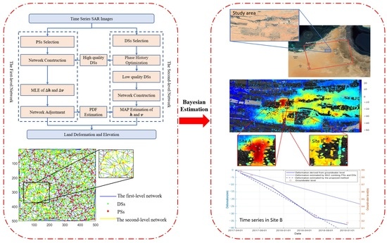
2.2. Bayesian Estimation of Land Deformation Combining Persistent and Distributed Scatterers

2.2.1. MAP Estimation of Deformation Parameters Based on Bayesian Theory

The main problem with the MLE is that the accuracy of the parameter estimation is greatly affected by the size and quality of the observation data, which means that the result of the parameter estimation is sensitive to random variations in the observation data. To deal with this, prior probabilities $\mathrm{P}\left(\mathit{x}\right)$ are introduced to improve the accuracy of the MLE. According to Bayesian theory, the posterior can be written as a product of likelihood and prior

$$\mathrm{P}\left(\mathit{x}|\mathit{y}\right)=\frac{\mathrm{P}\left(\mathit{y}|\mathit{x}\right)\mathrm{P}\left(\mathit{x}\right)}{\mathrm{P}\left(\mathit{y}\right)},$$

(10)

where $\mathrm{P}\left(\mathit{y}\right)$, called the probability of the observed data, is a normalizing constant ensuring that the posterior distribution has an area of 1. Then, we replace the likelihood with the posterior in the MLE in Equation (2), and we obtain the MAP estimation as in [38] by

$$\underset{\mathit{x}}{\mathrm{argmax}}\mathrm{P}\left(\mathit{y}|\mathit{x}\right)\mathrm{P}\left(\mathit{x}\right)=\underset{\Delta h,\Delta v}{\mathrm{argmax}}\left|\frac{1}{N}{\displaystyle \sum }_{n=1}^N\exp \left(-j{\phi }_n\left(\Delta h,\Delta v\right)\right)\right|\mathrm{P}\left(\Delta h,\Delta v\right),$$

(11)

where $\mathrm{P}\left(\Delta h,\Delta v\right)$ is the prior joint probabilities of $\Delta h$ and $\Delta v$.

The MAP estimation provides a framework for regularizing the tendency to match exactly with the observed data thus leading to a less noisy estimation. Moreover, MAP pulls the estimation towards the prior to an extent, which depends on the strength and bias of the prior relative to the likelihood.

As shown in Figure 2a, the MLE can achieve an unbiased estimation of $\Delta h$ and $\Delta v$ at (0, 0) without noise. However, as the noise increases, the temporal coherence decreases gradually and achieves the maximum of 0.6 at (2.8, −1.4) as shown in Figure 2b, and the MLE of $\Delta h$ and $\Delta v$ becomes worse. To improve the estimation accuracy of the MLE, the prior probabilities of $\Delta h$ and $\Delta v$ are given to achieve the MAP estimation. As shown in Figure 2c, the temporal coherence has greater kurtosis, and the MAP estimation is much better than the MLE in the case of unbiased Gaussian distribution for the priori probabilities. When the priori probabilities are biased slightly, the estimation accuracy of MAP will decline, but it is still better than the MLE as shown in Figure 2d. Thus, the priori probabilities of $\Delta h$ and $\Delta v$ determine the accuracy of the MAP estimation, and the PDF estimation method is given in the next subsection.

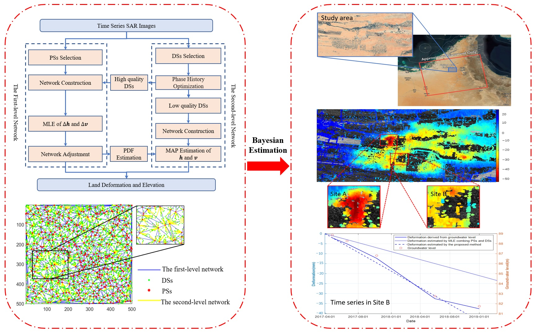
2.2.2. Two-Level Network for Deformation Parameters Estimation

• The first-level network for reliable scatterers

A two-level network is introduced into the traditional PSI to deal with PSs and DSs. In the first-level network, the deformation parameters at PSs and high-quality DSs are obtained accurately based on the Maximum Likelihood Estimation (MLE).

Given a stack of $N+1$ coregistered SAR images, PSs are first selected using the amplitude dispersion method [7,8,9]. Meanwhile, DSs are selected to increase the density of the measuring points. The DSs, affected by temporal and spatial decorrelation, are much noisier than the PSs, so the phase history of DSs is optimized using the PTA [15].

Unlike the traditional PS–DS algorithm, the DSs are divided into high-quality DSs and low-quality DSs according to the posterior coherence factors ${\rho }_{PTA\_\mathrm{H}}$ and ${\rho }_{PTA\_L}$, respectively. The high-quality DSs and PSs are jointly processed in the Delaney triangle network. Due to the noise of these points being very small, the MLE can obtain reliable estimation results in the arcs. Then, the linear deformation rate can be solved using the weighted least-square adjustment method [32]

$$\mathrm{X}={\left({\mathrm{B}}^{T}PB\right)}^{-1}{\mathrm{B}}^{T}PL,$$

(12)

where $\mathrm{X}$ is the vector of the deformation rates for the $M$ reliable points, $L=\left[\Delta {\widehat{v}}_1\Delta {\widehat{v}}_2\cdots \Delta {\widehat{v}}_Q\right]$ is the vector of the deformation rate difference of the $Q$ arcs, and $\mathrm{B}$ is the coefficient matrix composed of 1 and −1 and has the form

$$\mathrm{B}={\left[\begin{array}{c}1\\ 0\\ ⋮\\ 0\end{array}\begin{array}{c}0\\ 0\\ ⋮\\ 1\end{array}\begin{array}{c}-1\\ \dots \\ ⋮\\ 0\end{array}\begin{array}{c}0\\ 1\\ ⋮\\ -1\end{array}\begin{array}{c}0\\ -1\\ ⋮\\ 0\end{array}\right]}_{Q\times M},$$

(13)

where 1 represents the starting point and −1 corresponds to the ending point along each arc and $P$ is the weight matrix composed of the MTC

$$P={\left[\begin{array}{c}{\mathsf{\gamma }}_{MTC\_1}^2\\ 0\\ ⋮\\ 0\end{array}\begin{array}{c}0\\ {\mathsf{\gamma }}_{MTC\_2}^2\\ ⋮\\ 0\end{array}\begin{array}{c}0\\ \dots \\ ⋮\\ 0\end{array}\begin{array}{c}0\\ 0\\ ⋮\\ {\mathsf{\gamma }}_{MTC\_Q}^2\end{array}\right]}_{Q\times Q},$$

(14)

The residual elevation for reliable points can also be solved using the same process as above and $L=\left[\Delta {\widehat{h}}_1\Delta {\widehat{h}}_2\cdots \Delta {\widehat{h}}_Q\right]$ is the vector of the residual elevation difference of the $Q$ arcs.

• PDF estimation based on the Kriging model

Based on the results estimated from the first-level network and the spatial correlation of deformation field and elevation, the PDF of the deformation and elevation parameters at the low-quality DSs can be obtained using the Kriging model.

Kriging method, namely the Gaussian process regression method, is a geostatistical interpolation technology, which can give the best linear unbiased prediction at the unsampled locations according to the empirical observations [39]. In addition to a predicted value, it also provides the attached prediction error variance. The variance increases for predictions away from the data and as the spatial correlation weakens. Assuming that the output predicted values are $h_{prior}$ and $v_{prior}$ and the variances are ${\sigma }_h$ and ${\sigma }_v$, respectively, the prior joint Gaussian distribution for $h$ and $v$ can be expressed as

$$\mathrm{P}\left(h,v\right)=\frac{1}{2\pi {\sigma }_h{\sigma }_v}exp\left[-\frac{1}{2}\left(\frac{{\left(h-h_{prior}\right)}^2}{{\sigma }_h^2}+\frac{{\left(v-v_{prior}\right)}^2}{{\sigma }_v^2}\right)\right].$$

(15)

• The second-level network for the remaining DSs

In the second-level network, to restrain the error propagation of low-quality DSs in the adjustment network, the low-quality DSs are connected to the nearest PSs or high-quality DSs in the second-level network. Additionally, to improve the estimation accuracy, the deformation parameters of the low-quality DSs are estimated using MAP based on Bayesian theory.

Assuming that the deformation parameters of the nearest reliable scatterers are $h_r$ and $v_r$ according to Equations (11) and (15), the MAP estimation can be written as

$$\Delta h_{MAP},\Delta v_{MAP}=\underset{\Delta h,\Delta v}{\mathrm{argmax}}\left\{\left|\frac{1}{N}{\displaystyle \sum }_{n=1}^N\exp \left(-j{\phi }_n\left(\Delta h,\Delta v\right)\right)\right|·\mathrm{P}\left(\Delta h+h_r,\Delta v+v_r\right)\right\},$$

(16)

and the MAP estimation of the remaining DSs can be calculated directly by

$$v_{MAP}=\Delta v_{MAP}+v_r,$$

(17)

$$h_{MAP}=\Delta h_{MAP}+h_r.$$

(18)

The processing workflow of the proposed Bayesian estimation of land deformation combining PSs and DSs is shown in Figure 3.

3. Analysis and Results

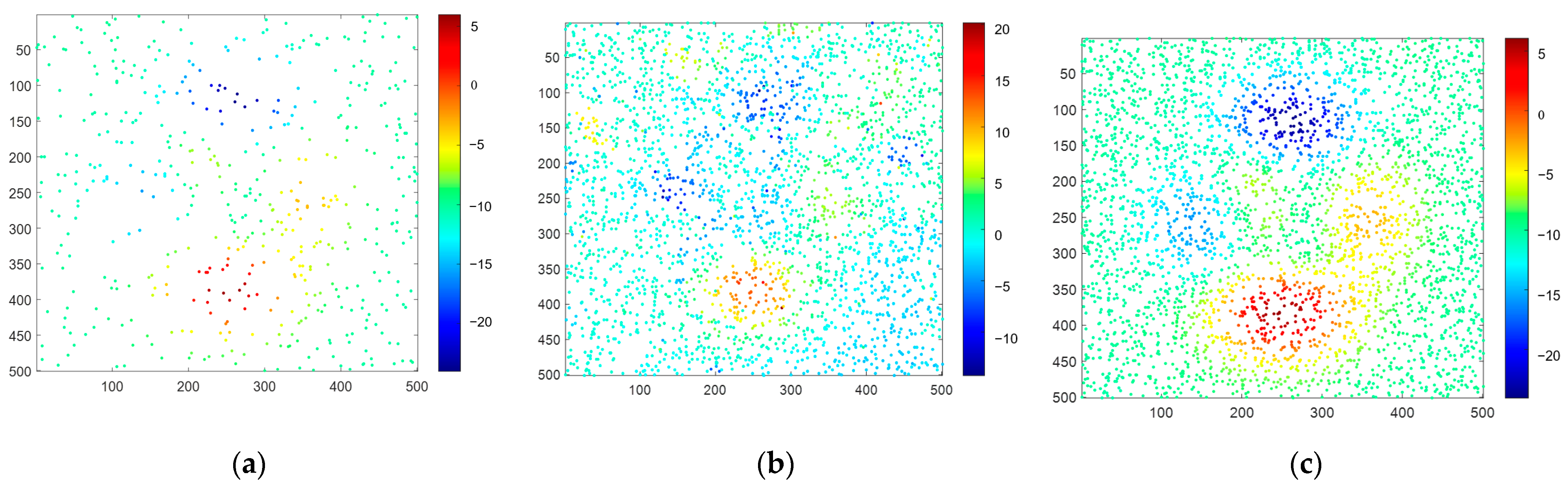
To validate the feasibility of the proposed method and assess its performance, two experiments are conducted based on simulated data and the Sentinel-1 real data set. Moreover, to show the reliability of the proposed method, the processing results are compared with the traditional PS–DS processing method using the MLE.

3.1. Simulated Data

A stack of 20 interferograms (with a size of 500 × 500) is generated in an existing single-master baseline configuration of the Sentinel-1A data with a time span of one year. The simulated phase consists of the deformation signals, residual elevation errors, and atmospheric phases, as shown in Figure 4a–c, respectively. Then, 450 PS pixels and 3000 DS pixels were simulated randomly in the study area, as shown in Figure 5. As mentioned above, the PSs and DSs with different scattering mechanisms have different noise levels. Therefore, the random noises with a standard deviation of 15 degrees and 45 degrees are added to the PS pixels and DS pixels (after PTA), respectively.

The deformation rates estimated using PSI, MLE combining PSs and DSs, and the proposed method are shown in Figure 6a–c, respectively. It can be seen that the deformation field in the PSI is in good agreement with the simulated deformation rates. However, due to the low density of PSs, many details are missing. The MLE combining PSs and DSs can increase the density of the measuring points. However, due to the poor phase quality of DSs in the simulation and the diffusion of arc errors in the adjustment network, the inversion results in some areas cannot accurately reflect the real deformation field. The proposed method not only greatly increases the density of the measuring points, but also ensures measurement accuracy and contains more detailed information.

Figure 7 shows the performance of the MLE combining PSs and DSs and the proposed method under different noise levels of DSs. In the MLE combining PSs and DSs, the arc measurements with poor estimation are discarded by setting the threshold of the MTC to 0.75 [31]. However, this operation cannot completely eliminate the influence of overwhelming outliers or decorrelation noise. When the phase quality of DSs deteriorates by more than 35 degrees, the measurement accuracy and measuring points of the MLE combining PSs and DSs will decrease sharply. As a comparison, the proposed method can still ensure the measurement accuracy and measuring points in the case of serious noise, which confirms the robustness of the proposed method. This shows that the proposed method is more robust, especially in low coherent areas such as rural areas, vegetation coverage areas, or deserts.

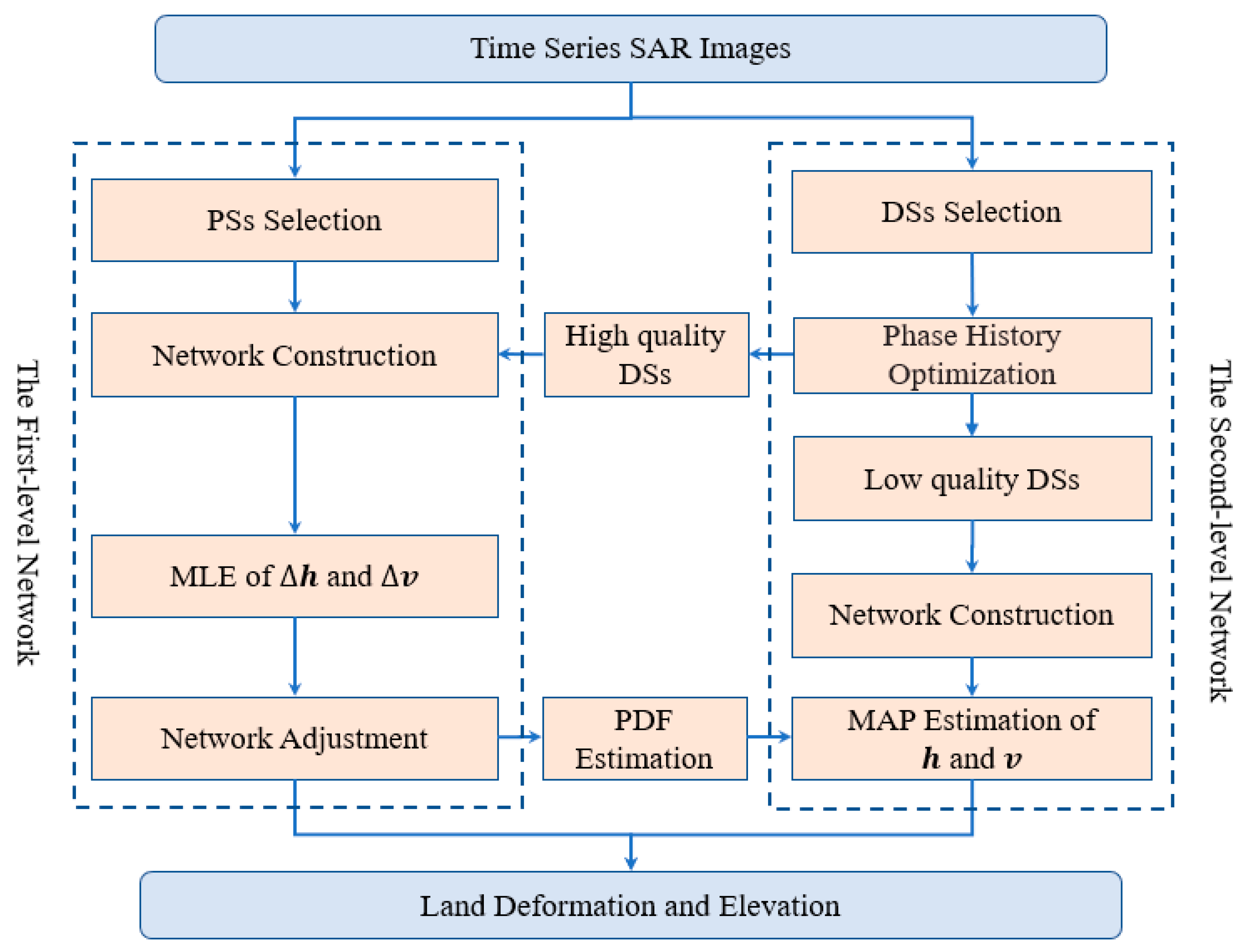
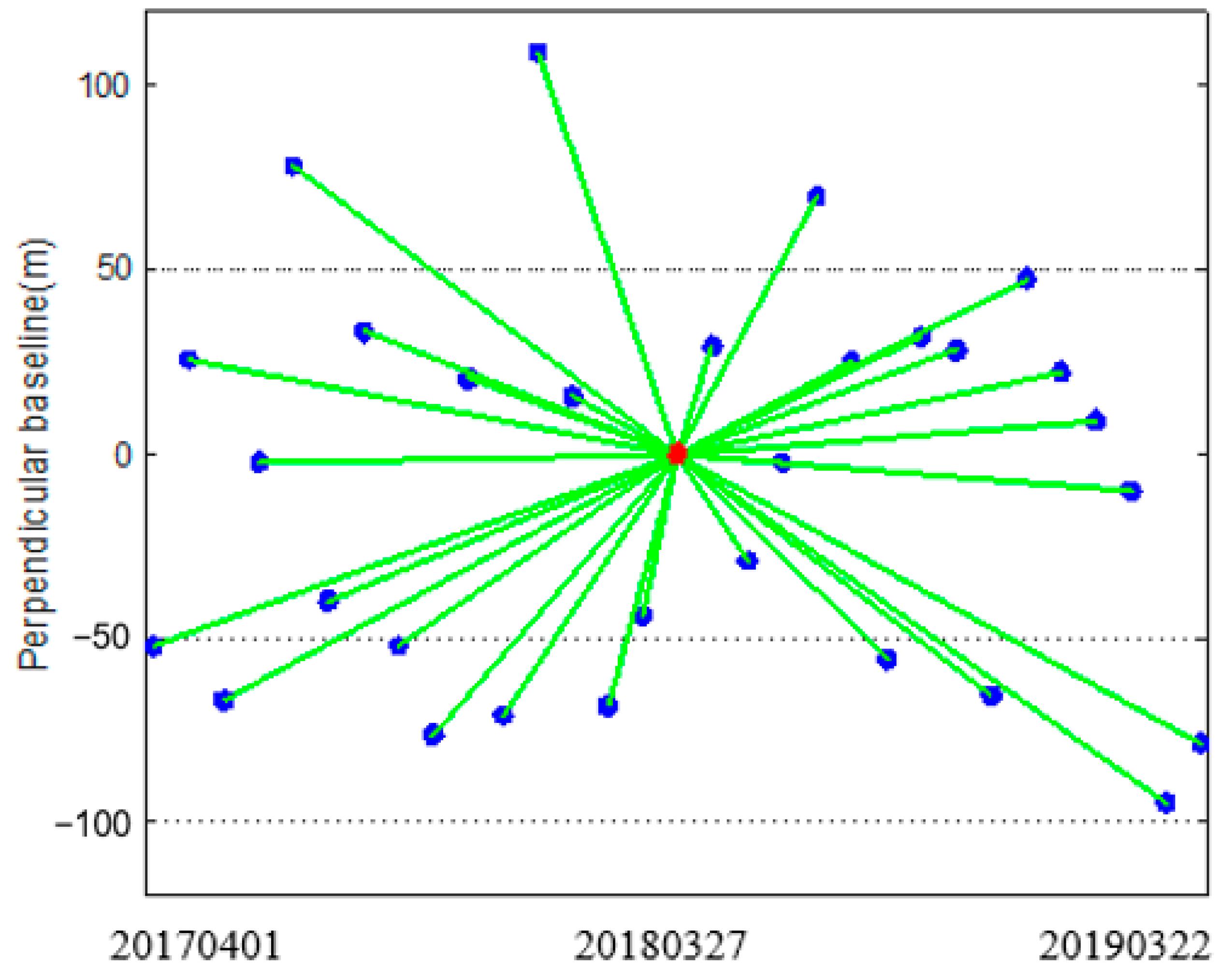
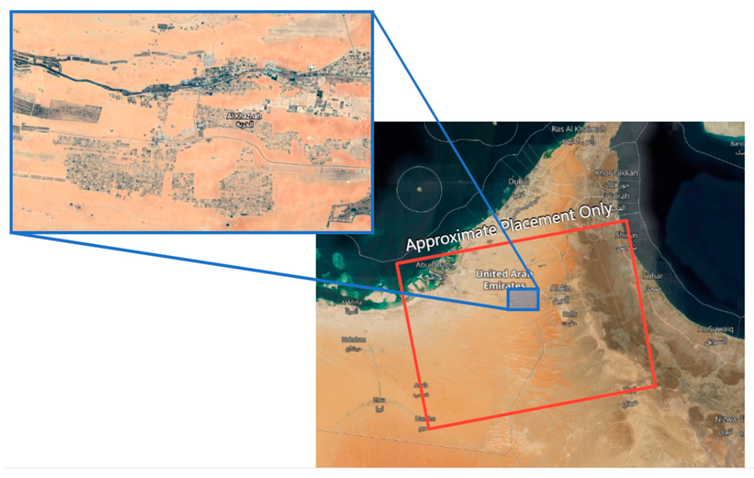
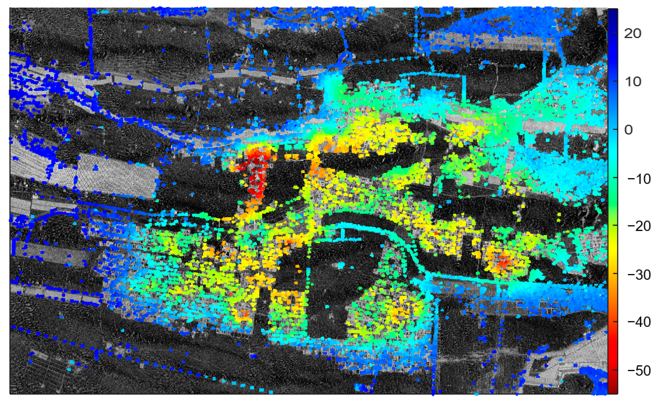
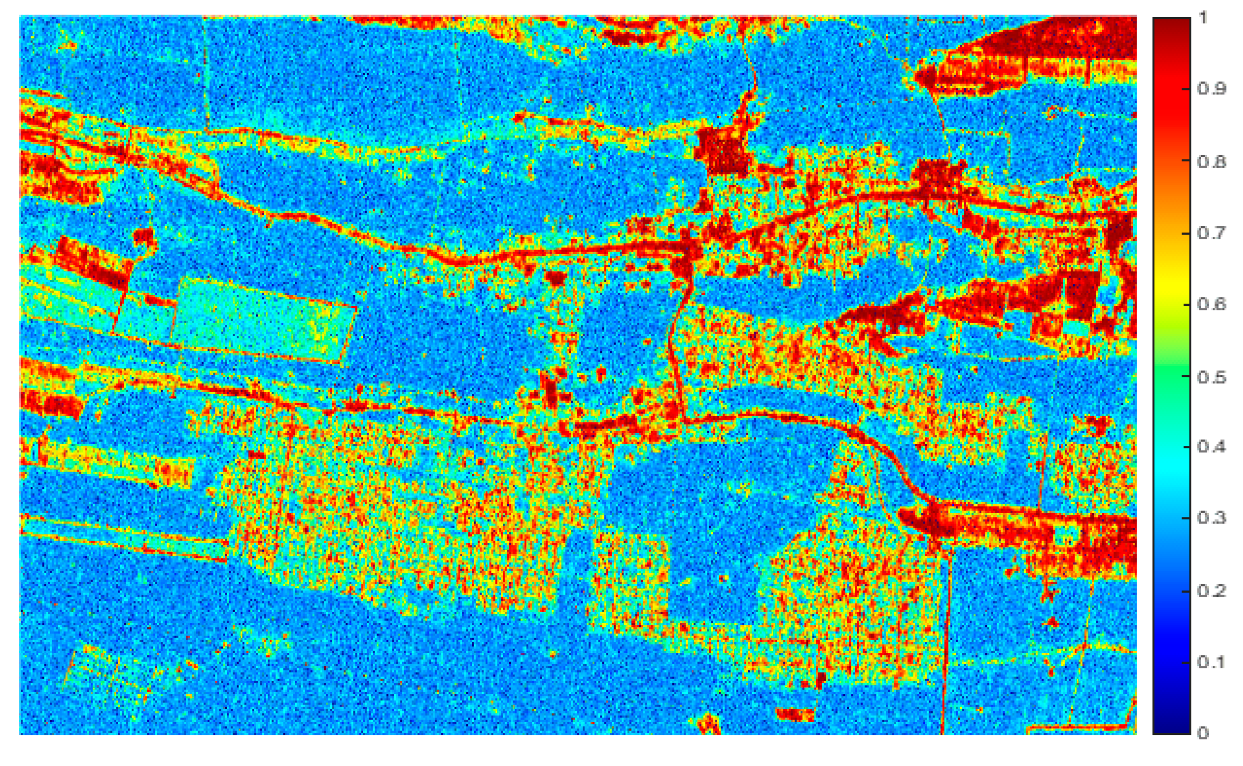
3.2. Real Data Set: Sentinel-1

Further validation of the proposed method was carried out by the experiments using a stack of 31 C-band Sentinel-1A SAR images in VV polarization from 1 April 2017 to 22 March 2019. The spatial-temporal baseline configuration is shown in Figure 8.

The test site is located at Remah in the United Arab Emirates (UAE), as shown in Figure 9, a place in an arid desert where rainfall is scarce and groundwater is the only source of natural freshwater. There are many farms and plantation forests in the study area. Groundwater abstraction for agricultural or human use has a significant impact on groundwater resources. As water is pumped from a well, it causes a drawdown of the aquifer water level nearby. According to the survey [40], there are about 4175 operational wells in Al Khaznah and about 232 mio m³ groundwater is abstracted every year. Agriculture and forests account for about 94% of the total annual groundwater use.

Abstracting groundwater leads to a depression of the groundwater surface around the well (the cone of depression). The map of groundwater level changes shows the groundwater level change from 2005 to 2017, which coincides with the agricultural areas [40,41]. At the test site, the groundwater level drops more than 14 m by monitoring the wells. In 2019, a cone-shaped water level was formed and the maximum drawdown at its center is approximately 40 to 50 m.

To explore the land deformation due to groundwater level drops, PSI technology is first adopted. As shown in Figure 10, the deformation rates estimated using PSI indicate that a subsidence bowl with a diameter of about 30 km is formed and the maximum deformation rate is about 55 mm/year, which is caused by the drawdown of the groundwater piezometric level. The PS pixels were selected using amplitude dispersion with a threshold of 0.25, and about 84,753 PSs are selected over the whole area of about 700 km². Therefore, the PS density is about 120 PSs/km². The arc measurements with an MTC less than 0.75 are discarded. The MTC of all available arcs has a mean value as high as 0.925. Therefore, the deformation rates using PSI are convincible.

Due to the common phenomenon of spatial-temporal decorrelation, it was difficult to obtain sufficient and effective PSs. To extract information from DSs and increase the spatial density of the measured points, PTA is performed to reduce the stochastic noise in DSs [15]. Based on the intensity image set and backscattering coefficient, the SHP is firstly selected, as shown in Figure 11. The selection window size is 11 × 21 and the SHP number threshold is set to 25. Based on the SHP family, the optimum phase values of DSs in time series are estimated using the MLE on all interferograms [15]. As shown in Figure 12, compared with the original phase, the signal-to-noise ratio (SNR) of the optimum phase values has been greatly improved, which proves the effectiveness of the PTA operation. The quality of the estimated phase of DSs can be indicated by the temporal coherence ${\mathsf{\gamma }}_{PTA}$, which can be used effectively for the final selection of DSs with reliable phase estimation, as shown in Figure 13. In the traditional PS–DS algorithm (MLE combining PSs and DSs), the threshold is set to 0.6. However, unlike the traditional PS–DS algorithm, the proposed method divided the DSs into high-quality DSs and low-quality DSs according to the posterior coherence factor ${\rho }_{PTA\_\mathrm{H}}=0.75$ and ${\rho }_{PTA\_L}=0.6$, respectively.

Then, the deformation rates were also estimated using the MLE combining PSs and DSs and the proposed method, as shown in Figure 14 and Figure 15, respectively. It can be seen that the PS–DS results contain much more detailed information in comparison with the counterpart outcomes of PSI. Both the MLE combining PSs and DSs and the proposed method can reflect the depression cone correlated with the groundwater level. However, in analogy to the simulated experiment, the deformation rates estimated using the MLE combining PSs and DSs are not consistent with the results estimated using PSI in some PS pixels, as shown in the bottom row of Figure 14. There are some unexpected variations from pixel to pixel due to the poor phase quality of DSs and the diffusion of arc errors in the adjustment network, as shown in the red oval box in Figure 14. Moving on to the results estimated using the proposed method, the deformation rates are highly consistent with the results using PSI and the outliers are significantly suppressed by the employment of prior information derived from the high-quality results using PSI.

According to the survey in Refs. [40,41], the spatial distribution of the land deformation fits with the area affected by the overexploitation of the aquifers. Moreover, there is a strong positive relationship between the groundwater level drawdown in the wells and the land subsidence in the time series. When the water level in the well drops by about 10 m, the surface settlement is about 50 mm [41]. From 1 April 2017 to 22 March 2019, the groundwater level time series in region B can be monitored by the water level of the well in region B. The mean deformation rates are calculated in region B of Figure 14 and Figure 15 and they are 12 mm/year and 25 mm/year, respectively.

As shown in Figure 16, the red circle is the groundwater level date of the GWP-060 monitoring well [41]. As mentioned earlier, due to the overexploitation of agricultural water, the groundwater level decreased significantly from May 2017 to January 2019, by up to about 8 m. According to the relationship between groundwater level and land subsidence, the land subsidence in the time series can be deduced, as shown by the solid blue line in Figure 16. The dotted blue line and dashed blue line are the deformation rates estimated using the MLE combining PSs and DSs and the proposed method, respectively. It is obvious that the deformation rate estimated using the proposed method is in good agreement with that of the groundwater level. However, the deformation rate estimated using the MLE combining PSs and DSs is too small, which is inconsistent with the groundwater level. The causes of the phenomenon are the poor phase quality of DSs in region B, which is reflected in the low temporal coherence value in Figure 13 and the error propagation in the subsequent adjustment network. In contrast, regularized by the spatial deformation field derived by the high-quality PSs and DSs, the proposed method achieves robust results even in the low coherence area.

4. Discussion

The results demonstrated the potential of the proposed method for measuring land deformation velocity in low coherence areas. Especially in rural areas, vegetation coverage areas, or deserts, the temporal decorrelation is particularly serious. Even after PTA processing, the phase quality of a large number of DSs is far inferior to that of PSs, which deteriorates the deformation measurement accuracy. The proposed method regularized by the spatial deformation field has better robustness in low coherence areas, and while ensuring the measurement accuracy, the number of measurement points can be greatly increased.

The spatial deformation field is derived from PSs and high-quality DSs in the first-level network. Thus, the proposed method is a model-free implementation and does not require the surface deformation pattern to be known before starting the data analysis. The land deformation measurement in the first-level network is crucial, which not only determines the accuracy of the measurement points in the primary network but also has a direct impact on the measurement in the secondary network. Therefore, when building the first-level network, we prefer reliable points. In some areas, there are few reliable points and the proposed method will also risk failure. It would be a good choice to obtain the information on the deformation field from other instruments as a priori input.

For our test site in the UAE, the land deformation presents as a subsidence bowl caused by the overexploitation of groundwater. This type of land deformation has a strong spatial correlation and is easier to derive accurately from the first-level network. Therefore, the proposed method is expected to perform well in strong spatial correlations of land deformation, such as mining subsidence, landslides, etc.

5. Conclusions

This paper proposes a Bayesian estimation method of land deformation combining PSs and DSs to solve the contradiction between measurement accuracy and coverage. A two-level network is introduced into the traditional PSI to deal with PSs and DSs. In the first-level network, the MLE of the deformation parameters at PSs and high-quality DSs are obtained accurately. In the secondary-level network, the remaining DSs are connected to the nearest PSs or high-quality DSs and the deformation parameters are estimated using MAP. Due to the poor phase quality of the remaining DSs, MAP can achieve better estimation results than the MLE based on the spatial correlation of the deformation field. The main advantage of the proposed method lies in its robustness despite the PTA phase estimation bias and the inconsistent noise levels due to the diffserent decorrelation mechanisms. Simulation and Sentinel-1A real data results verified the feasibility and reliability of the proposed method. A total of 31 Sentinel-1A SAR data acquired between 2017 and 2019 were exploited to detect the land deformation at Remah in the United Arab Emirates (UAE) caused by the overexploitation of the aquifers. The proposed method not only greatly increased the density of the measuring points, but also ensured measurement accuracy and contained more detailed information, which reflected the depression cone correlating with the groundwater level. Even in low coherence areas, the deformation rate estimated using the proposed method is in good agreement with that of the groundwater level. Moreover, the proposed method is a model-free implementation and does not require the surface deformation pattern to be known before starting the data analysis but is affected by the spatial correlation of land deformation. Therefore, in a strong spatial correlation of land deformation, such as groundwater-related subsidence, mining subsidence, landslides, etc., the proposed method is expected to perform well.

References

1. Bamler, R.; Hartl, P. Synthetic Aperture Radar interferometry. Inverse Probl. 1998, 14, R1. [Google Scholar] [CrossRef]
2. Gray, A.L.; Farris-Manning, P.J. Repeat-pass interferometry with Airborne Synthetic Aperture Radar. IEEE Trans. Geosci. Remote Sens. 1993, 31, 180–191. [Google Scholar] [CrossRef]
3. Goldstein, R. Atmospheric limitations to repeat-track radar interferometry. Geophys. Res. Lett. 1995, 22, 2517–2520. [Google Scholar] [CrossRef] [Green Version]
4. Zebker, H.A.; Villasenor, J. Decorrelation in interferometric radar echoes. IEEE Trans. Geosci. Remote Sens. 1992, 30, 950–959. [Google Scholar] [CrossRef] [Green Version]
5. Lavalle, M.; Simard, M.; Hensley, S. A temporal decorrelation model for polarimetric radar interferometers. IEEE Trans. Geosci. Remote Sens. 2012, 50, 2880–2888. [Google Scholar] [CrossRef]
6. Li, G.; Ding, Z.; Li, M.; Zhang, T.; Zeng, T.; Long, T. Earth-based repeat-pass SAR interferometry of the moon: Spatial–temporal baseline analysis. IEEE Trans. Geosci. Remote Sens. 2022, 60, 5227714. [Google Scholar] [CrossRef]
7. Ferretti, A.; Prati, C.; Rocca, F. Permanent scatterers in sar interferometry. IEEE Trans. Geosci. Remote Sens. 2001, 39, 8–20. [Google Scholar] [CrossRef]
8. Ferretti, A.; Prati, C.; Rocca, F. Nonlinear subsidence rate estimation using permanent scatterers in differential SAR interferometry. IEEE Trans. Geosci. Remote Sens. 2000, 38, 2202–2212. [Google Scholar] [CrossRef] [Green Version]
9. Hooper, A.; Segall, P.; Zebker, H. Persistent scatterer interferometric synthetic aperture radar for crustal deformation analysis, with application to Volcán Alcedo, Galápagos. J. Geophys. Res. 2007, 112, B07407. [Google Scholar] [CrossRef] [Green Version]
10. Crosetto, M.; Monserrat, O.; Cuevas-González, M.; Devanthéry, N.; Crippa, B. Persistent scatterer interferometry: A Review. ISPRS J. Photogramm. Remote Sens. 2016, 115, 78–89. [Google Scholar] [CrossRef] [Green Version]
11. Zhu, X.X.; Bamler, R. Very high resolution spaceborne sar tomography in urban environment. IEEE Trans. Geosci. Remote Sens. 2010, 48, 4296–4308. [Google Scholar] [CrossRef] [Green Version]
12. Guarnieri, A.M.; Tebaldini, S. On the exploitation of target statistics for SAR interferometry applications. IEEE Trans. Geosci. Remote Sens. 2008, 46, 3436–3443. [Google Scholar] [CrossRef]
13. Wang, Y.; Zhu, X.X.; Bamler, R. Retrieval of phase history parameters from distributed scatterers in urban areas using very high resolution SAR Data. ISPRS J. Photogramm. Remote Sens. 2012, 73, 89–99. [Google Scholar] [CrossRef] [Green Version]
14. Berardino, P.; Fornaro, G.; Lanari, R.; Sansosti, E. A new algorithm for surface deformation monitoring based on small baseline differential SAR interferograms. IEEE Trans. Geosci. Remote Sens. 2002, 40, 2375–2383. [Google Scholar] [CrossRef] [Green Version]
15. Ferretti, A.; Fumagalli, A.; Novali, F.; Prati, C.; Rocca, F.; Rucci, A. A new algorithm for processing interferometric data-stacks: Squeesar. IEEE Trans. Geosci. Remote Sens. 2011, 49, 3460–3470. [Google Scholar] [CrossRef]
16. Ho tong minh, D.; Hanssen, R.; Rocca, F. Radar Interferometry: 20 Years of development in time series techniques and future perspectives. Remote Sens. 2020, 12, 1364. [Google Scholar] [CrossRef]
17. Fan, H.; Lu, L.; Yao, Y. Method combining probability integration model and a small baseline subset for time series monitoring of mining subsidence. Remote Sens. 2018, 10, 1444. [Google Scholar] [CrossRef] [Green Version]
18. Hu, B.; Wang, H.-S.; Sun, Y.-L.; Hou, J.-G.; Liang, J. Long-term land subsidence monitoring of Beijing (China) using the small baseline subset (SBAS) technique. Remote Sens. 2014, 6, 3648–3661. [Google Scholar] [CrossRef] [Green Version]
19. Zhang, L.; Dai, K.; Deng, J.; Ge, D.; Liang, R.; Li, W.; Xu, Q. Identifying potential landslides by stacking-insar in southwestern China and its performance comparison with SBAS-Insar. Remote Sens. 2021, 13, 3662. [Google Scholar] [CrossRef]
20. Touzi, R. A review of speckle filtering in the context of estimation theory. IEEE Trans. Geosci. Remote Sens. 2002, 40, 2392–2404. [Google Scholar] [CrossRef]
21. Samiei-Esfahany, S.; Martins, J.E.; van Leijen, F.; Hanssen, R.F. Phase estimation for distributed scatterers in Insar stacks using integer least squares estimation. IEEE Trans. Geosci. Remote Sens. 2016, 54, 5671–5687. [Google Scholar] [CrossRef] [Green Version]
22. Shamshiri, R.; Nahavandchi, H.; Motagh, M.; Hooper, A. Efficient ground surface displacement monitoring using sentinel-1 data: Integrating Distributed Scatterers (DS) identified using two-sample t-test with persistent scatterers (PS). Remote Sens. 2018, 10, 794. [Google Scholar] [CrossRef] [Green Version]
23. Jiang, M.; Guarnieri, A.M. Distributed scatterer interferometry with the refinement of spatiotemporal coherence. IEEE Trans. Geosci. Remote Sens. 2020, 58, 3977–3987. [Google Scholar] [CrossRef]
24. Tebaldini, S.; Monti, A. Methods and performances for multi-pass SAR interferometry. In Geoscience and Remote Sensing New Achievements; InTech: London, UK, 2010; pp. 329–357. [Google Scholar] [CrossRef] [Green Version]
25. Wang, Y.; Zhu, X.X. Robust estimators for multipass SAR interferometry. IEEE Trans. Geosci. Remote Sens. 2016, 54, 968–980. [Google Scholar] [CrossRef]
26. Ansari, H.; De Zan, F.; Bamler, R. Efficient phase estimation for Interferogram Stacks. IEEE Trans. Geosci. Remote Sens. 2018, 56, 4109–4125. [Google Scholar] [CrossRef]
27. Jiang, M.; Ding, X.; Li, Z. Hybrid approach for unbiased coherence estimation for multitemporal insar. IEEE Trans. Geosci. Remote Sens. 2014, 52, 2459–2473. [Google Scholar] [CrossRef]
28. Wang, C.; Wang, X.S.; Xu, Y.; Zhang, B.; Jiang, M.; Xiong, S.; Zhang, Q.; Li, W.; Li, Q. A new likelihood function for consistent phase series estimation in distributed scatterer interferometry. IEEE Trans. Geosci. Remote Sens. 2022, 60, 5227314. [Google Scholar] [CrossRef]
29. Even, M.; Schulz, K. Insar deformation analysis with distributed scatterers: A review complemented by new advances. Remote Sens. 2018, 10, 744. [Google Scholar] [CrossRef] [Green Version]
30. Shi, G.; Lin, H.; Ma, P. A hybrid method for stability monitoring in low-coherence urban regions using persistent and distributed scatterers. IEEE J. Sel. Top. Appl. Earth Obs. Remote Sens. 2018, 11, 3811–3821. [Google Scholar] [CrossRef]
31. Du, Z.; Ge, L.; Ng, A.H.-M.; Zhang, Q.; Alamdari, M.M. Assessment of the accuracy among the common persistent scatterer and distributed scatterer based on Squeesar Method. IEEE Geosci. Remote Sens. Lett. 2018, 15, 1877–1881. [Google Scholar] [CrossRef]
32. Liang, H.; Zhang, L.; Ding, X.; Lu, Z.; Li, X.; Hu, J.; Wu, S. Suppression of coherence matrix bias for phase linking and ambiguity detection in mtinsar. IEEE Trans. Geosci. Remote Sens. 2021, 59, 1263–1274. [Google Scholar] [CrossRef]
33. Guarnieri, A.M.; Tebaldini, S. Hybrid cramér–Rao bounds for crustal displacement field estimators in sar interferometry. IEEE Signal Process. Lett. 2007, 14, 1012–1015. [Google Scholar] [CrossRef]
34. Agram, P.S.; Simons, M. A noise model for Insar Time Series. J. Geophys. Res. Solid Earth 2015, 120, 2752–2771. [Google Scholar] [CrossRef]
35. Zhang, L.; Ding, X.; Lu, Z. Modeling PSInSAR time series without phase unwrapping. IEEE Trans. Geosci. Remote Sens. 2011, 49, 547–556. [Google Scholar] [CrossRef]
36. Morishita, Y.; Hanssen, R.F. Temporal decorrelation in L-, C-, and X-band satellite radar interferometry for pasture on drained peat soils. IEEE Trans. Geosci. Remote Sens. 2015, 53, 1096–1104. [Google Scholar] [CrossRef]
37. Kellndorfer, J.; Cartus, O.; Lavalle, M.; Magnard, C.; Milillo, P.; Oveisgharan, S.; Osmanoglu, B.; Rosen, P.A.; Wegmüller, U. Global Seasonal sentinel-1 interferometric coherence and backscatter data set. Sci. Data 2022, 9, 73. [Google Scholar] [CrossRef]
38. Gauvain, J.-L.; Lee, C.-H. Maximum a posteriori estimation for multivariate gaussian mixture observations of Markov chains. IEEE Trans. Speech Audio Process. 1994, 2, 291–298. [Google Scholar] [CrossRef]
39. Oliver, M.A.; WEBSTER, R. Kriging: A method of interpolation for Geographical Information Systems. Int. J. Geogr. Inf. Syst. 1990, 4, 313–332. [Google Scholar] [CrossRef]
40. Groundwater Atlas of Abu Dhabi Emirate. Available online: https://www.researchgate.net/publication/337936386_GROUNDWATER_ATLAS_OF_ABU_DHABI_EMIRATE (accessed on 5 July 2022).
41. El Kamali, M.; Papoutsis, I.; Loupasakis, C.; Abuelgasim, A.; Omari, K.; Kontoes, C. Monitoring of land surface subsidence using persistent scatterer interferometry techniques and ground truth data in arid and semi-arid regions, the case of Remah, UAE. Sci. Total Environ. 2021, 776, 145946. [Google Scholar] [CrossRef]
Figure 1. Temporal coherence and CRB of the preprocessed phase of DSs. (a) Temporal coherence model in urban, pasture, and water areas; (b) The CRB standard deviations of the preprocessed phase of DSs and the standard deviation of a typical PS (∼ 25 ° ) are also plotted.
Remotesensing 14 03471 g001
Figure 2. Estimation of Δ h and Δ v : (a) MLE without noise: γ M T C = 1, Δh = 0, Δv = 0; (b) MLE with noise: γ M T C = 0.6, Δ h ^ = 2.8, Δ v ^ = −1.4; (c) MAP estimation with noise: Δ h ^ = 0.2, Δ v ^ = 0 and unbiased prior: Δh~N(0,9), Δv~N(0,4); (d) MAP estimation with noise: Δ h ^ = 0.8, Δ v ^ = 0.6 and biased prior: Δh~N(1,9), Δv~N(1,4).
Remotesensing 14 03471 g002
Figure 3. The processing workflow of the proposed method.
Remotesensing 14 03471 g003
Figure 4. The simulated phase consists of (a) the deformation signals (mm/year); (b) residual elevation errors (m); and (c) atmospheric phases (rad).
Remotesensing 14 03471 g004
Figure 5. The proposed two-level network combining PSs and DSs.
Remotesensing 14 03471 g005
Figure 6. Deformation rates estimated using (a) PSI, (b) MLE combining PSs and DSs, and (c) the proposed method.
Remotesensing 14 03471 g006
Figure 7. The performance comparison of the proposed method and MLE combining PSs and DSs.
Remotesensing 14 03471 g007
Figure 8. The baseline configuration of the used data set.
Remotesensing 14 03471 g008
Figure 9. The test site located at Remah.
Remotesensing 14 03471 g009
Figure 10. The land deformation estimated using PSI.
Remotesensing 14 03471 g010
Figure 11. The SHP numbers.
Remotesensing 14 03471 g011
Figure 12. The original and optimum phase of DSs.
Remotesensing 14 03471 g012
Figure 13. Temporal coherence map γ P T A .
Remotesensing 14 03471 g013
Figure 14. The land deformation estimated using MLE combining PSs and DSs. (A) Site A, (B) Site B.
Remotesensing 14 03471 g014
Figure 15. The land deformation estimated using the proposed method. (A) Site A, (B) Site B.
Remotesensing 14 03471 g015
Figure 16. The correlation between the groundwater level and land deformation.
Remotesensing 14 03471 g016
Publisher’s Note: MDPI stays neutral with regard to jurisdictional claims in published maps and institutional affiliations.