Rapid Linear Frequency Swept Frequency-Modulated Continuous Wave Laser Source Using Iterative Pre-Distortion Algorithm

Abstract

We present a simple iterative pre-distortion algorithm for achieving a rapid linear frequency sweep of semiconductor lasers. The algorithm achieves the desired frequency swept linearity with only four iterations. We derive a general formula for iterative pre-distortion by establishing the relationship between the laser output frequency and the drive current. The linear frequency-swept laser source obtained by this algorithm can be used in FMCW LiDAR systems. Experimentally, we investigated the algorithm using a 1550 nm distributed feedback (DFB) laser, achieving frequency swept excursion of 30.26 GHz, and frequency swept slope of 504 THz/s. We analyzed the linearity of the frequency swept results for the fourth iteration, achieving less than 5 MHz root mean square (RMS) value of frequency swept nonlinearity.

1. Introduction

Light detection and ranging (LiDAR) technologies have many applications in three-dimensional (3D) imaging systems [1,2], autonomous driving [3,4], remote sensing [5,6] and other domains. In general, there are two different categories of LiDAR, one is pulsed time-of-flight (TOF) LiDAR and the other is frequency modulated continuous wave (FMCW) LiDAR. Compared to TOF LiDAR, FMCW LiDAR uses coherent detection [7,8,9] to extract frequency information, thus it can be immune to direct sun light and interference from other LiDAR transmitters [3]. However, there is an unique advantage for a specially designed FMCW LiDAR which can simultaneously measure the 3D positions and one dimensional speed of a target in a single measurement spot so that it is often called four-dimensional (4D) measurement LiDAR [10,11].

There is a linearly frequency-swept laser source in a FMCW LiDAR system as an emitter of which three optical parameters significantly determine the performance of the LiDAR [12]. One is the coherent length or linewidth of the frequency-swept light source determines the maximum detection distance that a FMCW LiDAR can reach. The second one is the frequency swept excursion of the laser source which determines the distance resolution. The larger the frequency sweep excursion, the higher distance resolution is. The last one is the most important for a LiDAR which is frequency swept linearity of the laser source because it related to the ranging accuracy of the FMCW LiDAR directly.

In order to obtain a high linearity of the frequency swept light wave, the most effective method is to modulate a semiconductor laser externally [13]. However, a broadband arbitrary waveform generator (AWG) is required as a necessary piece of equipment for generating a broadband ideal linearly frequency swept electrical signal that leads to a kind of light source which is too bulky and too expensive. Another method that generates linearly frequency swept light waves is called an electrical driving semiconductor laser, directly or internally [14,15], which does not require expensive AWG. Therefore, this method has received a large amount of attention. For most semiconductor lasers, however, the frequency of the output does not change linearly with the injected drive current to the laser [16,17]. Especially at high repetition rate of injected drive current, a significant nonlinearity of the frequency-time curve cannot be avoided, which means that is impossible to maintain a high ranging accuracy in this sort of FMCW LiDAR [18].

There are two main approaches to fix the problem in an internal drive semiconductor laser system, especially when the semiconductor laser itself is a distributed feedback laser diode (DFB-LD) [16,19]. One is to use a phase-locked loop (PLL) to drive a DFB-LD for generation of a perfect linearly frequency-swept light waves, and the other is use an open electric circuit to drive a DFB-LD based on a pre-distortion technique. However, for the closed PLL, the frequency swept rate has to be pretty slow due to the intrinsic relaxation oscillation effect of a DFB-LD. For example, the group in the Montana State University generated a linearly frequency swept light source within a broad excursion of 4.8 THz in 800 ms, of which the frequency swept slope is only 6 THz/s at the extremely low repetition rate of 1.25 Hz [14]. Obviously, it is not practical for detection of a moving target. Pre-distortion techniques usually involve mathematical modeling of the system and then experimental optimization of the parameters. Minissale et al. used γ correction techniques [20] by establishing a power function relationship between the laser output frequency and the drive voltage, and experimentally determining the control parameters to achieve a frequency swept nonlinearity correction [21]. Karlsson measured the response of the laser at different modulation frequencies and compensated for the nonlinearity by building a linear time-invariant model of the laser using a pre-distortion technique [22]. Yao et al. used a digitally integrated, self-training method to generate the pre-distortion curves, but the method requires a long convergence time [23].

Several typical applications of iterative pre-distortion techniques have been published recently. Wu’s group at UC Berkeley succeeded in generation of a linearly frequency swept output from a DFB-LD based on the pre-distortion technique, so called iterative learning control approach, at the repetition rate of 4 kHz over the swept excursion of 45 GHz with the frequency swept slope of 360 THz/s [19]. Chen’s group in Tsinghua University improved the linearly frequency-swept system with a homemade chip device using the similar pre-distortion method [24]. The repetition rate is 1 kHz and frequency swept excursion is 5.6 GHz so that the maximum frequency swept slope is about 11.1 THz/s. Wu’s group at Shanghai Jiao Tong University proposes a novel method that combines an inverse function pre-distortion algorithm with an iterative algorithm for linearly frequency-swept [25]. The repetition rate is 1 kHz and the frequency swept excursion is 26 GHz, and the frequency swept slope of 52 THz/s.

In the above reported pre-distortion techniques, all of them use the iterative learning control method, and the residual nonlinearity reaches 1.8 × 10⁻⁸, and the root mean square value of the frequency swept nonlinearity is less than 1.5 MHz [19]. However, the convergence and convergence speed of this method strongly depend on the manually selected scale factor, and the optimal scale factor is different for different lasers, which needs to be obtained through a trial-and-error process several times. A similar approach was used by Ming H Chen et al. The laser source in the experiment consisted of a DFB-LD and an external micro-ring resonator (MRR), so the iterative learning control required consideration of thermal conduction effects, and the residual nonlinearity was less than 4.1 × 10⁻⁹ for 50 iterations of the method, and the RMS value of the frequency swept nonlinearity was suppressed to within 0.21 MHz [24]. The iterative algorithm of Wu Kan et al. usually requires the driving waveform obtained by the inverse function pre-distortion algorithm as the start of the iterative algorithm, and requires a suitable choice of coefficients for the exponential term in the iterative algorithm, which further increases the complexity of the algorithm. The residual nonlinearity reaches 5.19 × 10⁻⁸, and the root mean square value of the frequency swept nonlinearity is 1.5 MHz [25].

In this paper, a simple iterative pre-distortion method based on the zero-crossing method [26,27] is proposed to achieve a laser frequency swept linear output, and it is experimentally verified with a narrow linewidth DFB-LD of 1550 nm. After four pre-distortion iterations, the RMS value of the DFB-LD frequency swept nonlinearity is less than 5 MHz. The experimental results reach the expected requirements. This algorithm does not require complex control systems and tedious data post-processing to achieve frequency swept linearization, and is independent of the specific laser. This frequency swept linearization method opens up the application of FMCW laser sources and is particularly suitable for low-cost, easy-to-install, high-performance systems.

2. The Principle of DFB-LD Output Linearly Frequency-Swept Light Wave

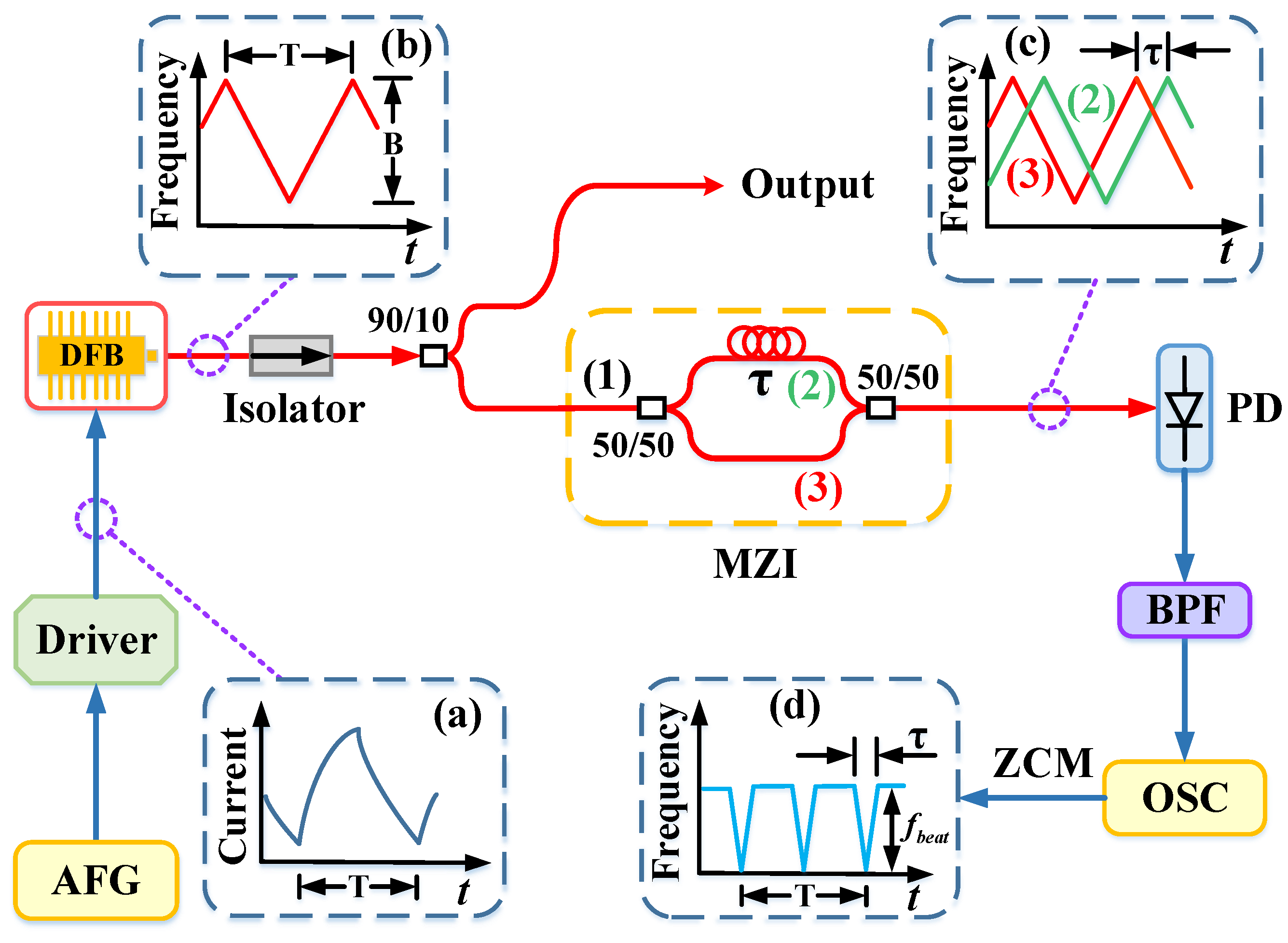
The schematic of implementing the DFB-LD linearly frequency-swept is shown in Figure 1. The drive current waveform obtained by the iterative pre-distortion algorithm that makes the DFB-LD linearly frequency swept is pre-input into the arbitrary function generator (AFG), and the drive module of the DFB-LD is synchronized with the AFG, the pre-distortion current that is injected into the DFB-LD is shown in Figure 1a. Under this current drive, the DFB-LD outputs the frequency swept light wave of the cycle, and its time-frequency curve is shown in Figure 1b. After passing through the isolator, the frequency swept light wave is divided into two beams by a 90:10 coupler. 90% of the light wave is output directly, and the other 10% is sent to an unbalanced fiber optic Mach-Zehnder interferometer (MZI) to generate autocorrelation external differential interference, and the time-frequency curves of the two-frequency swept light waves with differential time delay τ are shown in Figure 1c. The photodetector (PD) converts the two coherently superimposed light waves into electrical signals, which are acquired by an oscilloscope (OSC) after passing through a band-pass filter (BPF), and the time-frequency curves of the MZI beat signals are obtained by the zero-crossing method (ZCM) (see Figure 1d).

Assuming that the electric field of the frequency swept light wave at the input (1) of MZI in Figure 1 is

$$E(t)=A\cos \left[{\varphi }_{SFL}(t)\right]$$

(1)

where A denotes the field amplitude, ${\varphi }_{SFL}(t)$ denotes the phase of the DFB output light wave.

Assume that the laser output light wave frequency is

$${\omega }_{SFL}(t)={\omega }_0+{\xi }_d\cdot t$$

(2)

where ${\omega }_0$ is the light carrier frequency and ${\xi }_d$ is the linearly frequency swept slope, both of which are constants.

FMCW LiDAR requires the instantaneous frequency of the DFB-LD output light wave to vary linearly with time.

The phase in Equation (1) is expressed as

$${\varphi }_{SFL}(t)={\omega }_{0}t+\frac{1}{2}{\xi }_d{t}^2+\theta$$

(3)

where θ denotes the initial phase of the light wave.

At the unbalanced MZI emitting end, the total light intensity is obtained by coherent superposition of the two light fields expressed by Equation (4), which is expressed by Equation (5).

$$\begin{array}{l}{E}_1(t)=\frac{\sqrt{2}}{2}E(t-\tau )=\frac{\sqrt{2}}{2}A\cos \left[{\varphi }_{SFL}(t-\tau )\right]\\ E_2(t)=\frac{\sqrt{2}}{2}E(t)=\frac{\sqrt{2}}{2}A\cos \left[{\varphi }_{SFL}(t)\right]\end{array}$$

(4)

where τ is the fiber time delay of the unbalanced MZI.

$$I(t)={\left\{\frac{\sqrt{2}A}{2}\cos \left[{\varphi }_{SFL}(t-\tau )\right]+\frac{\sqrt{2}A}{2}\cos \left[{\varphi }_{SFL}(t)\right]\right\}}^2$$

(5)

The photocurrent signal output from PD is proportional to the light intensity. Since the high frequency component in Equation (5) is beyond the response range of the photodetector, and when the photocurrent signal passes through BPF, the expression of the photocurrent signal contains only the differential frequency component. Therefore, we can get the expression of photocurrent as

$$i_{beat}(t)\propto \frac{R{A}^2}{2}\cos [{\varphi }_{SFL}(t)-{\varphi }_{SFL}(t-\tau )]$$

(6)

where R is the responsiveness of the photodetector. The phase of the photocurrent is denoted as ${\varphi }_{beat}(t)$:

$${\varphi }_{beat}(t)={\varphi }_{SFL}(t)-{\varphi }_{SFL}(t-\tau )$$

(7)

When the time delay τ is sufficiently small, we can obtain the relationship as follows:

$${\varphi }_{beat}(t)={\varphi }_{SFL}(t)-{\varphi }_{SFL}(t-\tau )=\frac{d{\varphi }_{SFL}(t)}{dt}\tau$$

(8)

where $\frac{d{\varphi }_{SFL}(t)}{dt}$ is the instantaneous frequency ${\omega }_{SFL}(t)$ of the output light wave of the DFB-LD, and if ${\omega }_{SFL}(t)$ varies linearly with time, we get from Equation (2):

$$\frac{d{\varphi }_{SFL}(t)}{dt}=\frac{d({\omega }_{0}t+\frac{1}{2}{\xi }_d{t}^2+\theta )}{dt}={\omega }_0+{\xi }_{d}t={\omega }_{SFL}(t)$$

(9)

Thus, the phase ${\varphi }_{beat}(t)$ of the photocurrent can be expressed as

$${\varphi }_{beat}(t)={\omega }_{SFL}(t)\cdot \tau =\left({\omega }_0+{\xi }_d\cdot t\right)\cdot \tau ={\xi }_d\tau \cdot t+{\omega }_0\tau$$

(10)

The time derivative of Equation (10) yields the time-frequency curve ${\omega }_{beat}(t)$ of the photocurrent beat frequency signal.

$${\omega }_{beat}(t)=\frac{d{\varphi }_{beat}(t)}{dt}$$

(11)

Substitution of Equation (10) into Equation (11) reveals that the time-frequency curve ${\omega }_{beat}(t)$ of the photocurrent beat-frequency signal should be the same as Figure 1d, where the beat signal frequency is kept constant in an up or down-sweep period, noted as f_beat, which is equal to $\frac{{\xi }_d\tau }{2\pi }$.

However, the relationship between the instantaneous frequency ${\omega }_{SFL}(t)$ of the DFB-LD output light wave and the driving current of the DFB-LD is nonlinear, which can be expressed as

$${\omega }_{SFL}(t)={\omega }_0+K_{SFL}(i)\cdot i(t)$$

(12)

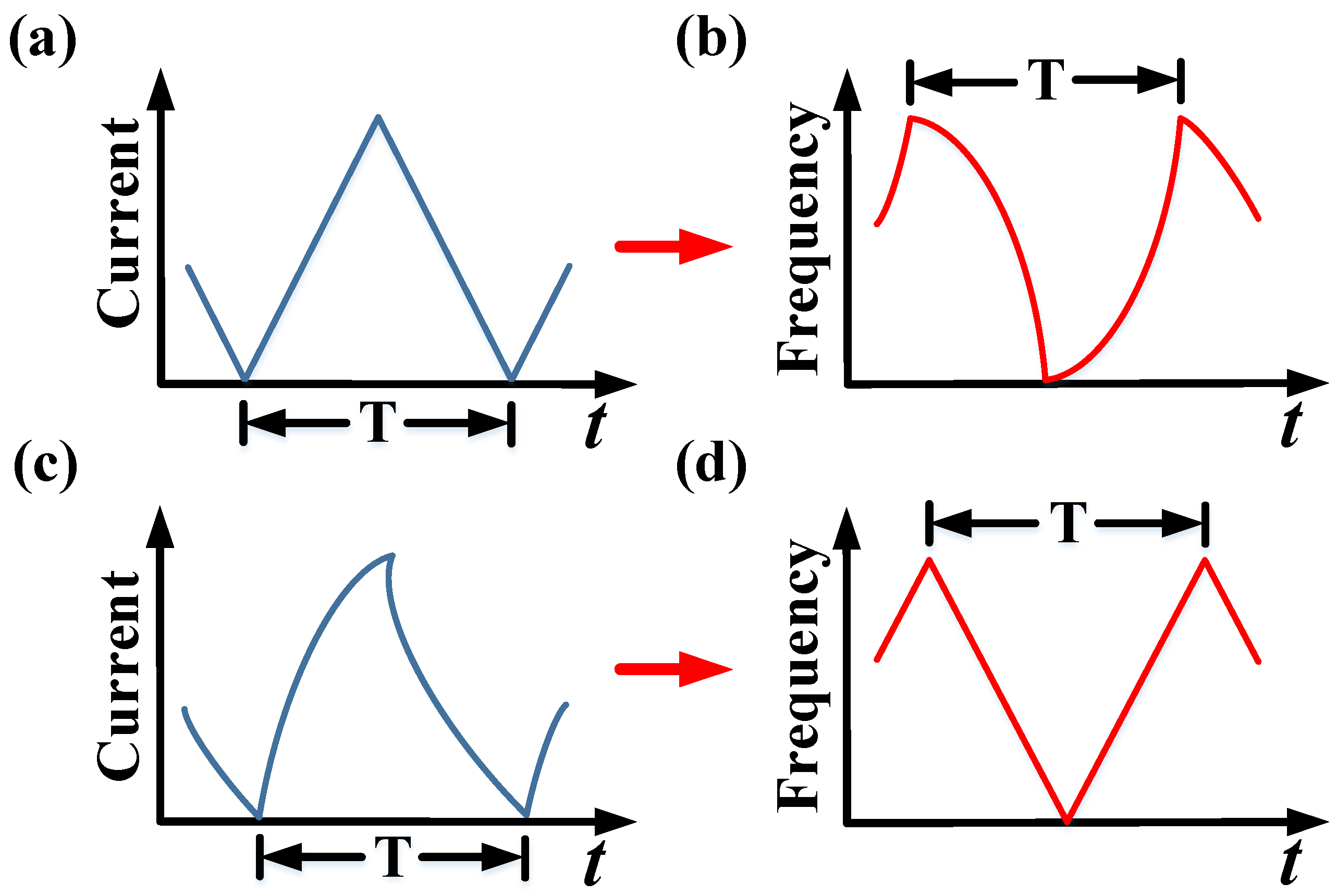
where i(t) is the driving current of the DFB-LD. K_SFL(i) is the proportionality factor, which is generally not a constant and can be seen as a function of the driving current i(t). As shown in Figure 2, when the drive current i(t) is an ideal triangular waveform as in Figure 2a, the output frequency ${\omega }_{SFL}(t)$ of the DFB-LD does no longer change linearly with time as ideal, but as shown in Figure 2b, which results in the time-frequency curve ${\omega }_{beat}(t)$ of the unbalanced MZI output beat-frequency signal is no longer constant ${\xi }_d\tau$. Therefore, the DFB-LD must be driven by a current with a distorted triangular waveform, namely pre-distortion technique, to achieve the DFB-LD linearly frequency swept output. In other words, pre-distortion is applied on the basis of the ideal triangular waveform to obtain a distorted triangular waveform current as shown in Figure 2c to drive the DFB-LD, aiming to make the time-frequency curve of the instantaneous frequency ${\omega }_{SFL}(t)$ of the output light waveform of the DFB-LD an ideal triangular waveform as shown in Figure 2d.

The method to determine the shape of the driving DFB-LD current (distorted triangular wave) is as follows.

Substituting Equation (8) into the instantaneous frequency of the photocurrent beat signal obtained from Equation (11), the time-frequency curve of the beat signal can be obtained proportional to the first-order derivative of the time-frequency curve of the DFB-LD, as shown in Equation (13).

$${\omega }_{beat}(t)=\frac{d{\varphi }_{beat}(t)}{dt}=\frac{d}{dt}\left[\frac{d{\varphi }_{SFL}(t)}{dt}\tau \right]=\tau \frac{d{\omega }_{SFL}(t)}{dt}$$

(13)

The scale factor K_SFL(i) in Equation (12) can be determined by substituting Equation (12) into Equation (13):

$${\omega }_{beat}(t)=\frac{di(t)}{dt}\left(\tau K_{SFL}+\tau i\frac{d{K}_{SFL}}{di}\right)=\frac{di(t)}{dt}\cdot F_{dist}(i)$$

(14)

where $F_{dist}(i)$ is a distortion function related to the scale factor K_SFL(i):

$$F_{dist}\left[i\left(t\right)\right]=\tau K_{SFL}+\tau i\frac{d{K}_{SFL}}{di}$$

(15)

It is obtained by several measurement and iterations. In addition, $F_{dist}(i)$ is also a function of time as the driving current i(t) varies with time.

We can drive the DFB-LD in Figure 1 with the continuously obtained pre-distortion driving current waveform through an iterative algorithm, so that the frequency ${\omega }_{beat}(t)$ of the photocurrent beat frequency signal constantly converges to a constant.

The specific iterative method starts from the ideal triangular wave driving current, let $\frac{di(t)}{dt}$ in Equation (14) be the constant ${\xi }_i$, i.e., apply the ideal triangular wave driving current to the DFB-LD, the photocurrent beat signal is recorded by the OSC in Figure 1, the instantaneous frequency ${\omega }_{beat}(t)$ of this signal is found by the zero-crossing method, and it is noted as ${\omega }_{beat}^{(0)}(t)$. Finally, the initial distortion function $F_{dist}\left[i(t)\right]$ can be calculated from Equation (14), denoted as $F_{dist}^{(0)}\left[i(t)\right]$.

$$F_{dist}^{(0)}\left[i\left(t\right)\right]=\frac{{\omega }_{beat}^{(0)}(t)}{{\xi }_i}$$

(16)

where ${\xi }_i$ is the slope of the triangular wave driving current, after which $F_{dist}^{(0)}\left[i(t)\right]$ is brought back to Equation (14), and the ${\omega }_{beat}(t)$ on the left side of the equal sign of Equation (14) is made equal to the constant $2\pi {\xi }_d\tau$ to obtain the following equation.

$${\xi }_d\tau =\frac{di(t)}{dt}\cdot F_{dist}^{(0)}\left[i\left(t\right)\right]$$

(17)

It can be known easily that Equation (17) is a first-order differential equation, and the integration gives the first-order pre-distortion drive current $i^{(1)}(t)$.

$$i^{(1)}(t)={\displaystyle \int \frac{{\xi }_d\tau }{F_{dist}^{(0)}\left[i\left(t\right)\right]}dt}$$

(18)

Input the obtained first-order pre-distortion drive current $i^{(1)}(t)$ into the AFG again to drive the DFB-LD in Figure 1, and record the photocurrent beat signal again, and obtain the time-frequency curve ${\omega }_{beat}^{(1)}(t)$ of the beat signal by the zero-crossing method. Apply Equation (14) again to find the first-order distortion function $F_{dist}^{(1)}\left[i(t)\right]$.

$$F_{dist}^{(1)}\left[i\left(t\right)\right]=\frac{{\omega }_{beat}^{(1)}(t)}{\frac{d{i}^{(1)}(t)}{dt}}=\frac{{\omega }_{beat}^{(1)}(t)}{\frac{{\xi }_d\tau }{F_{dist}^{(0)}\left[i\left(t\right)\right]}}=\frac{{\omega }_{beat}^{(1)}(t)}{{\xi }_d\tau }{F}_{dist}^{(0)}\left[i\left(t\right)\right]$$

(19)

The distortion function $F_{dist}^{(1)}\left[i(t)\right]$ is brought to Equation (14) again, solved for the first-order differential equation, and then the second-order pre-distortion drive current $i^{(2)}(t)$ is calculated.

$$i^{(2)}(t)={\displaystyle \int \frac{{\xi }_d\tau }{F_{dist}^{(1)}\left[i\left(t\right)\right]}dt}$$

(20)

The second-order pre-distortion drive current $i^{(2)}(t)$ is used to drive the DFB-LD again, thus obtaining the time-frequency curve ${\omega }_{beat}^{(2)}(t)$ of the beat signal and the second-order distortion function $F_{dist}^{(2)}\left[i(t)\right]$.

$$F_{dist}^{(2)}\left[i\left(t\right)\right]==\frac{{\omega }_{beat}^{(2)}(t)}{{\xi }_d\tau }{F}_{dist}^{(1)}\left[i\left(t\right)\right]$$

(21)

Iterate in accordance with this method until ${\omega }_{beat}^{(N)}(t)$ converges to a constant ${\xi }_d\tau$, at which point the drive current $i^{(N)}(t)$ is

$$i^{(N)}(t)={\displaystyle \int \frac{{\xi }_d\tau }{F_{dist}^{(N-1)}\left[i\left(t\right)\right]}dt}$$

(22)

where $F_{dist}^{(N-1)}\left[i(t)\right]$ is

$$F_{dist}^{(N-1)}\left[i\left(t\right)\right]=\frac{{\omega }_{beat}^{(N-1)}(t)}{{\xi }_d\tau }{F}_{dist}^{(N-2)}\left[i\left(t\right)\right]\approx F_{dist}^{(N-2)}\left[i\left(t\right)\right]$$

(23)

3. Experimental Results of Pre-Distortion Current Drive DFB-LD Output Frequency Swept Light Wave

The experimental system used a commercial narrow linewidth DFB-LD laser with a linewidth of 157 kHz, center wavelength of 1550 nm, and maximum output power of 75 mW. The differential time delay time of the MZI two-arm fiber is 4.66 ns. The delay fiber length is sufficiently small, the MZI employs a polarization-preserving fiber, and it is vibration isolated, so that the delay time t can be assumed to be completely constant with time. The beat signal was acquired by an OSC (MSOS804A, Keysight Technologies, Santa Rosa, CA, USA). 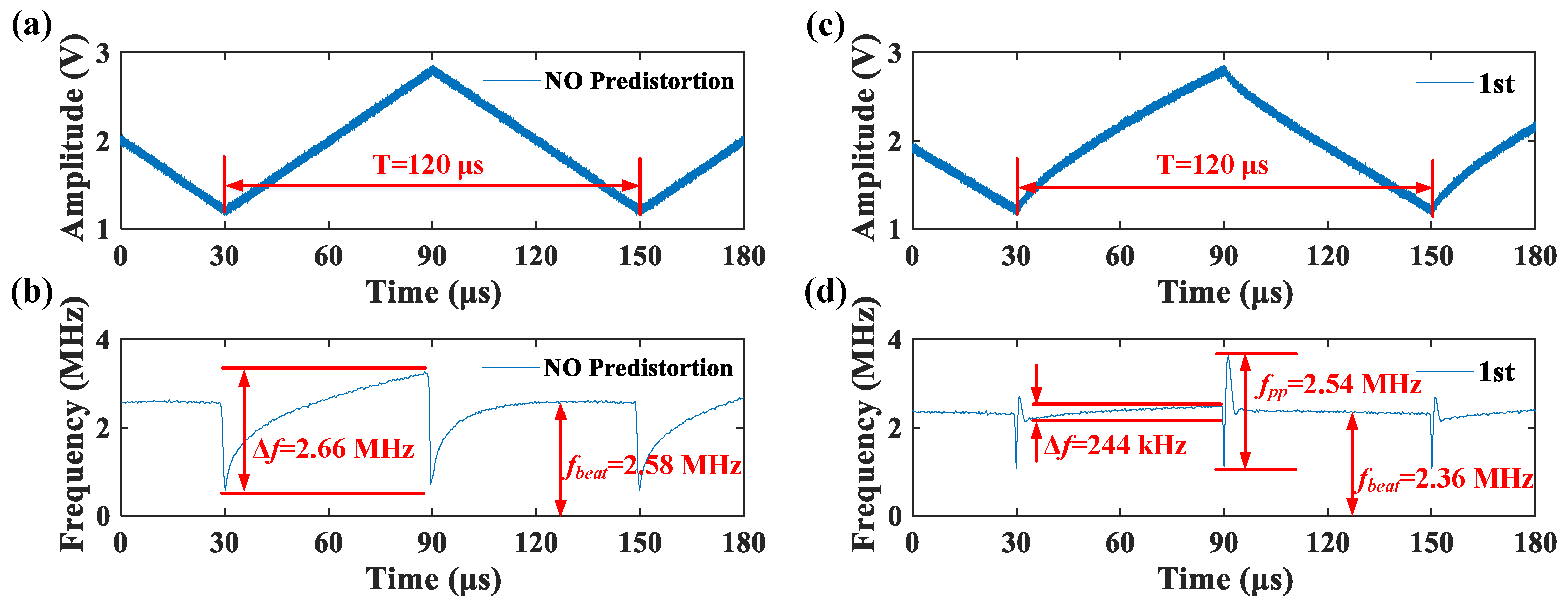The corresponding time-frequency curve ${\omega }_{beat}(t)$ was calculated by the zero-crossing method. During the experiments, the sampling rate of the oscilloscope is usually set to be 2 GS/s. The drive current waveform is preset into AFG (AFG3252, Tektronix), and the voltage output signal of the AFG modulates the drive module of the DFB-LD. The bias current of the DFB-LD is 200 mA and the amplitude is ±80 mA. According to the correspondence between current and voltage, the bias voltage applied by AFG to the laser driver is 2 V and the amplitude is ±800 mV. The initial input voltage is a standard triangular wave, and the modulation period of the triangular wave is 120 μs, as shown in Figure 3a.

When the no pre-distortion triangular waveform shown in Figure 3a is injected into the drive module of the DFB-LD, the time-frequency curve of the beat signal at the MZI output will deviate from the ideal constant frequency. As shown in Figure 3b, the time-frequency curve varies slowly with time over a wide bandwidth ∆f (2.66 MHz). This indicates that the frequency of the DFB-LD is not linear with time; this conclusion is also verified later in Figure 5a.

Figure 3c shows the drive voltage waveform obtained after the 1st pre-distortion, which obviously deviates from the ideal triangular waveform. As can be seen in Figure 3d, the corresponding ∆f of the time-frequency curve of the beat signal is greatly reduced to 244 kHz. The 10 times optimization of ∆f indicates that our pre-distortion method is effective. It is noticeable that there is a frequency mutation at the transition between the up and down-sweep in Figure 3d. The frequency peak-to-peak value f_pp is 2.54 MHz. This is caused by the unique laser relaxation oscillation effect of DFB-LD, which can be attenuated by special design of the shape of the driving current inflection point. During the experiments, only 80% of the light waves in the linearly frequency-swept range are utilized, and the LiDAR data generated by light waves output near the current inflection point are automatically screened out and not counted as valid data.

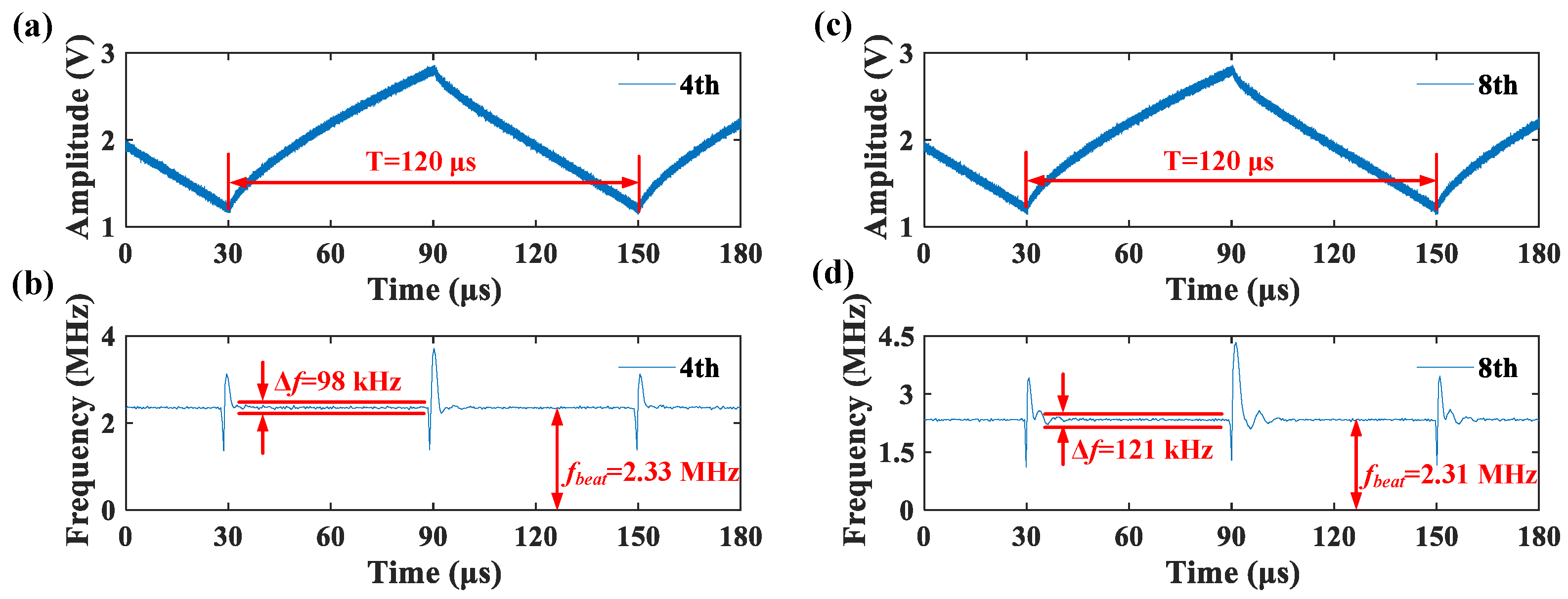
After more iterations of pre-distortion, the linearity of the frequency variation of the DFB-LD output light wave with time becomes higher and higher. Figure 4b shows the experimental results of the 4th iteration, which shows that the ∆f is reduced by another 2.5 times, from 244 kHz to 98 kHz. However, higher orders of iterations do not necessarily lead to better results. As shown in Figure 4d, the frequency variation range ∆f has increased slightly to 121 kHz. This may be attributed to the accumulation of multiple iterations. During each iteration operation, the 40-cycle signal acquired by the OSC are filtered and smoothed for improvement of the accuracy of the zero-crossing method. Meanwhile, some of valid data are also filtered, resulting in the deviation from the optimal solution.

In order to calculate the time frequency curve of the frequency swept light wave output by the DFB-LD under current drive, we extract the phase ${\varphi }_{beat}(t)$ of the beat frequency signal by Hilbert transform (HT). 40-period beat signal of the MZI output obtained from the OSC are used to obtain the time frequency curve $f_{SFL}(t)$ of the frequency swept light wave by direct calculation of Equation (10); Figure 5a,d, respectively. Figure 5a,d shows the frequency swept results of the laser output light wave driven by the no pre-distortion triangular waveform voltage and the 4th pre-distortion voltage, respectively. 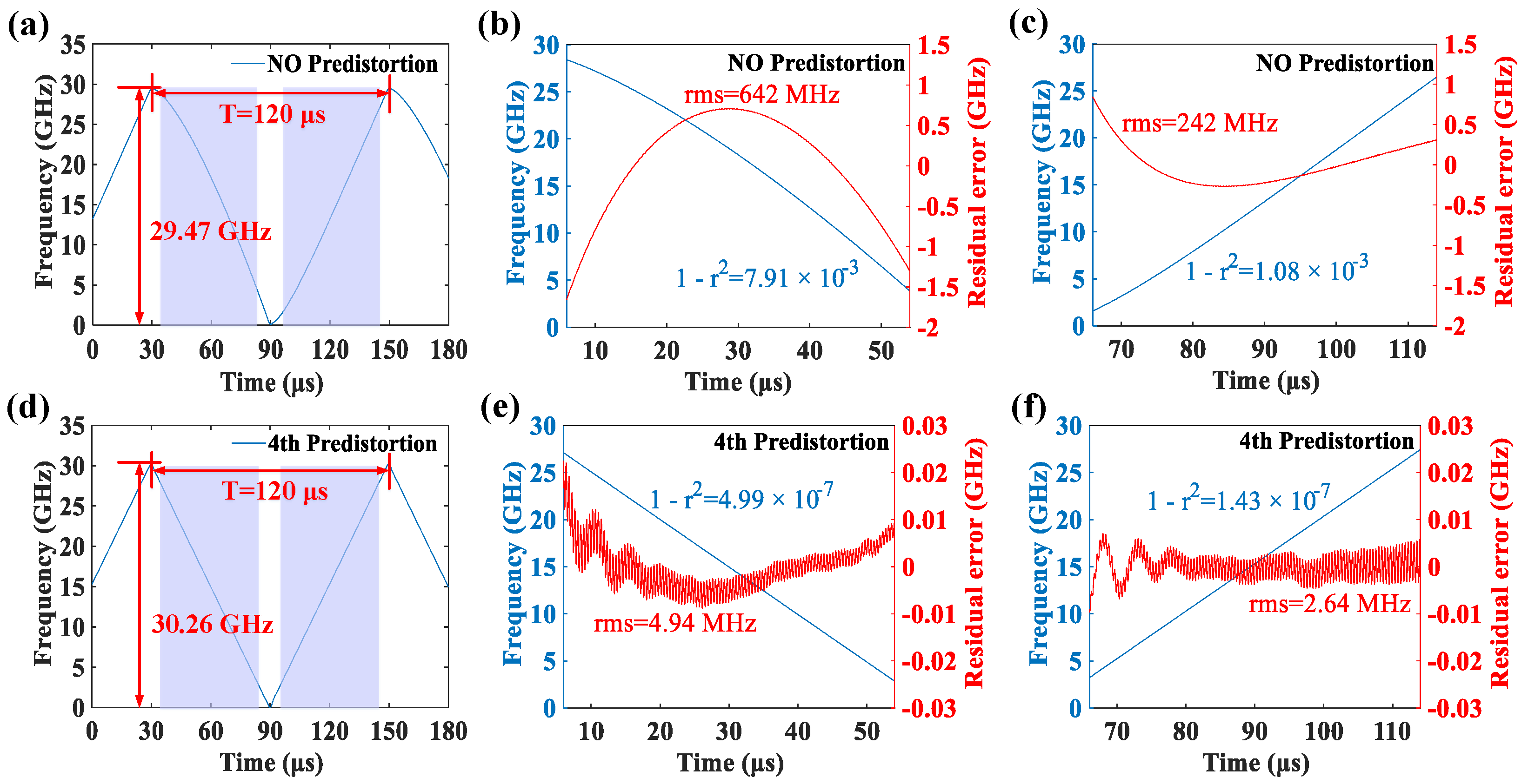Figure 5a,d show the frequency swept light wave of 180 us, which contains a complete frequency swept process. As shown in Figure 5a, the frequency swept waveform has a large nonlinearity under the no-predistortion triangular voltage drive, especially in the initial part where the frequency swept slope is flipped, and the frequency swept bandwidth is 29.47 GHz. As shown in Figure 5d, the frequency swept nonlinearity has been corrected more under the fourth-order predistortion voltage drive, and the frequency swept bandwidth is increased to 30.26 GHz.

In Figure 5a, the frequency of the DFB-LD output light wave shows a significant nonlinearity with time driven by the no pre-distortion triangular waveform voltage. To characterize the magnitude of this nonlinearity, we select 80% of the up and down-sweep regions in the DFB-LD frequency swept range as the effective region, as the shaded region in Figure 5a. The linearity of the laser frequency swept can also be expressed by the linear regression coefficient r² = 1 − SS_res/SS_tot, where SS_res residual sum of squares, SS_tot total sum of squares, r² is a constant less than 1, the higher the linearity the closer to 1, we adopted 1 − r² to represent the residual nonlinearity. The $1-r^2$ and the RMS value $f_{nl,rms}$ of the frequency swept nonlinearity in these two effective regions are calculated and shown in Figure 5b,c, respectively. It can be seen that $1-r^2$ for the down and up-sweep is 0.00791 and 0.00108, respectively, both at 10⁻³ level. The corresponding $f_{nl,rms}$ is 642 MHz and 242 MHz, both in the order of a few hundred MHz. As we expected, the situation has improved significantly after the 4th iteration. The linearity of the frequency swept is enhanced obviously, as show in Figure 5d. Both $1-r^2$ reaching the 10⁻⁷ level in the same shaded region is an improvement of 4 orders of magnitude. $f_{nl,rms}$ is also reduced by two orders of magnitude, in the order of a few MHz (see Figure 5e,f).

It is worth mentioning that our method is able to achieve the DFB-LD linearly frequency-swept light wave output with a minimum number of iterations. In Figure 6, the $1-r^2$ of the down and up-sweep of a different iteration number is given. As can be seen from the figure, the best results appear in the 4th iteration, but when the number of iterations exceeds the 4th, the frequency swept linearity deteriorates because noise is introduced at each iteration with the algorithm, and with the accumulation of noise leads to a change in the trend of the frequency swept nonlinearity towards deterioration. Therefore, the 4th pre-distortion waveform is selected as the final drive voltage for linearly frequency-swept output, in our experiments.

4. Conclusions

In this paper, we propose an iterative pre-distortion algorithm to achieve high performance frequency swept linearization, and demonstrate that the iterative pre-distortion algorithm can be used to correct the frequency swept nonlinearity of the laser with DFB-LD at 1550 nm. Through multiple experiments and analysis, the best frequency swept linearization is achieved at the 4th iteration. When the laser is driven with the pre-distortion current generated by the 4th iteration, a linear frequency change of 30.26 GHz can be achieved in 60 μs. We have obtained satisfactory results with iterative pre-distortion algorithms. Nevertheless, as we expected, the frequency swept curve of the DFB-LD output light wave is not completely linear. The algorithm provides a realistic basis for the next step of application of an optoelectronic phase-locked loop to achieve accurate linear frequency swept.