
Lidar-Based Aboveground Biomass Estimations for the Maya Archaeological Site of Yaxnohcah, Campeche, Mexico

 , and
, and
Abstract
:
1. Introduction
2. Materials and Methods
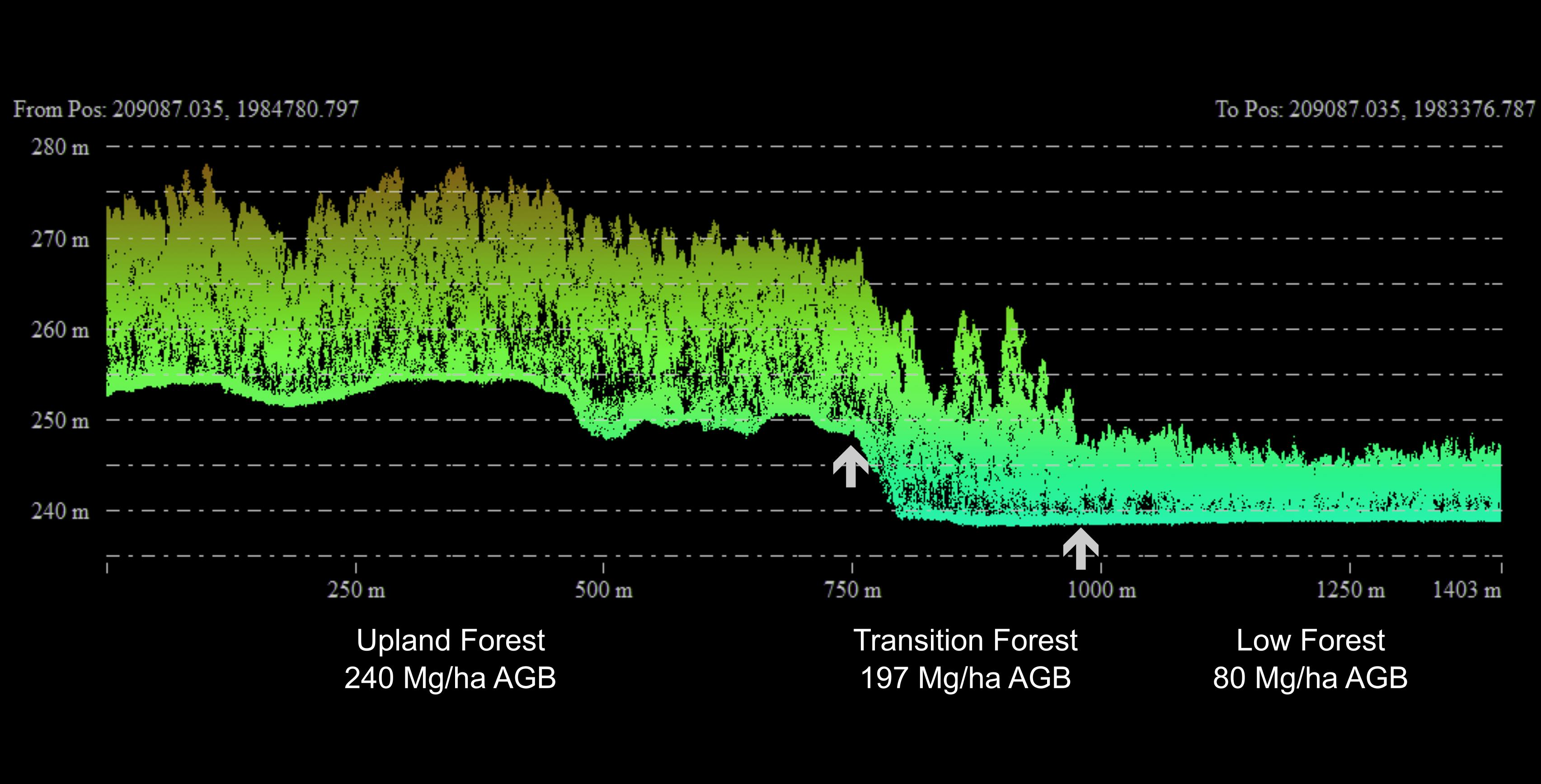
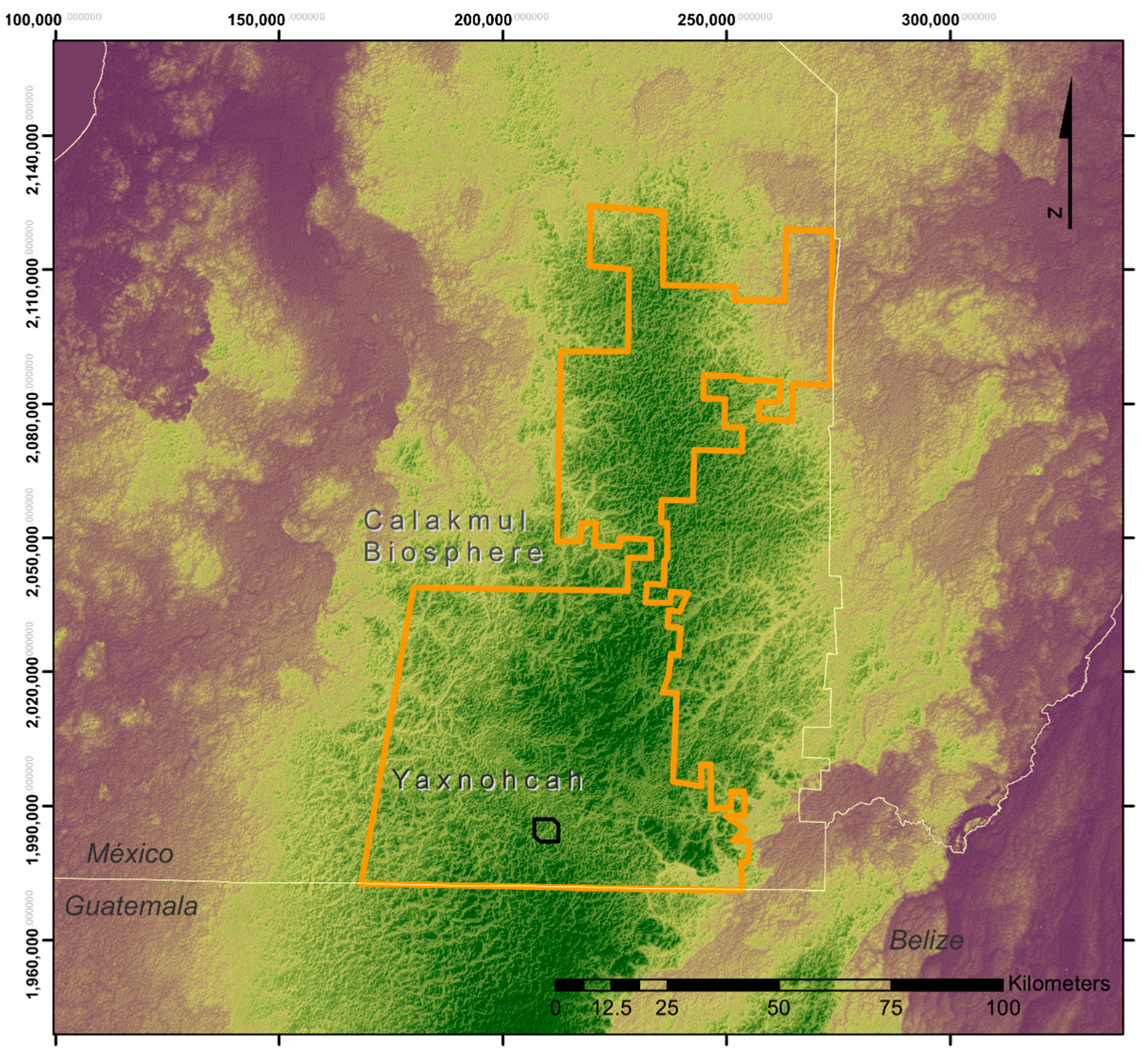
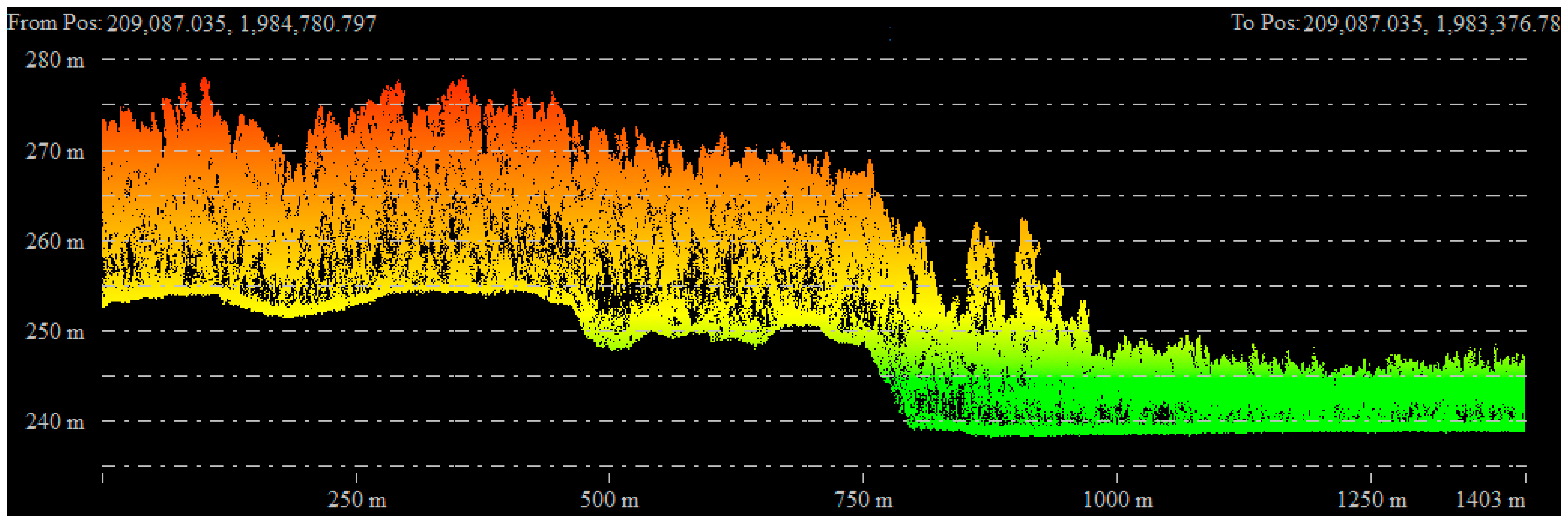
2.1. Survey Area and Landscape
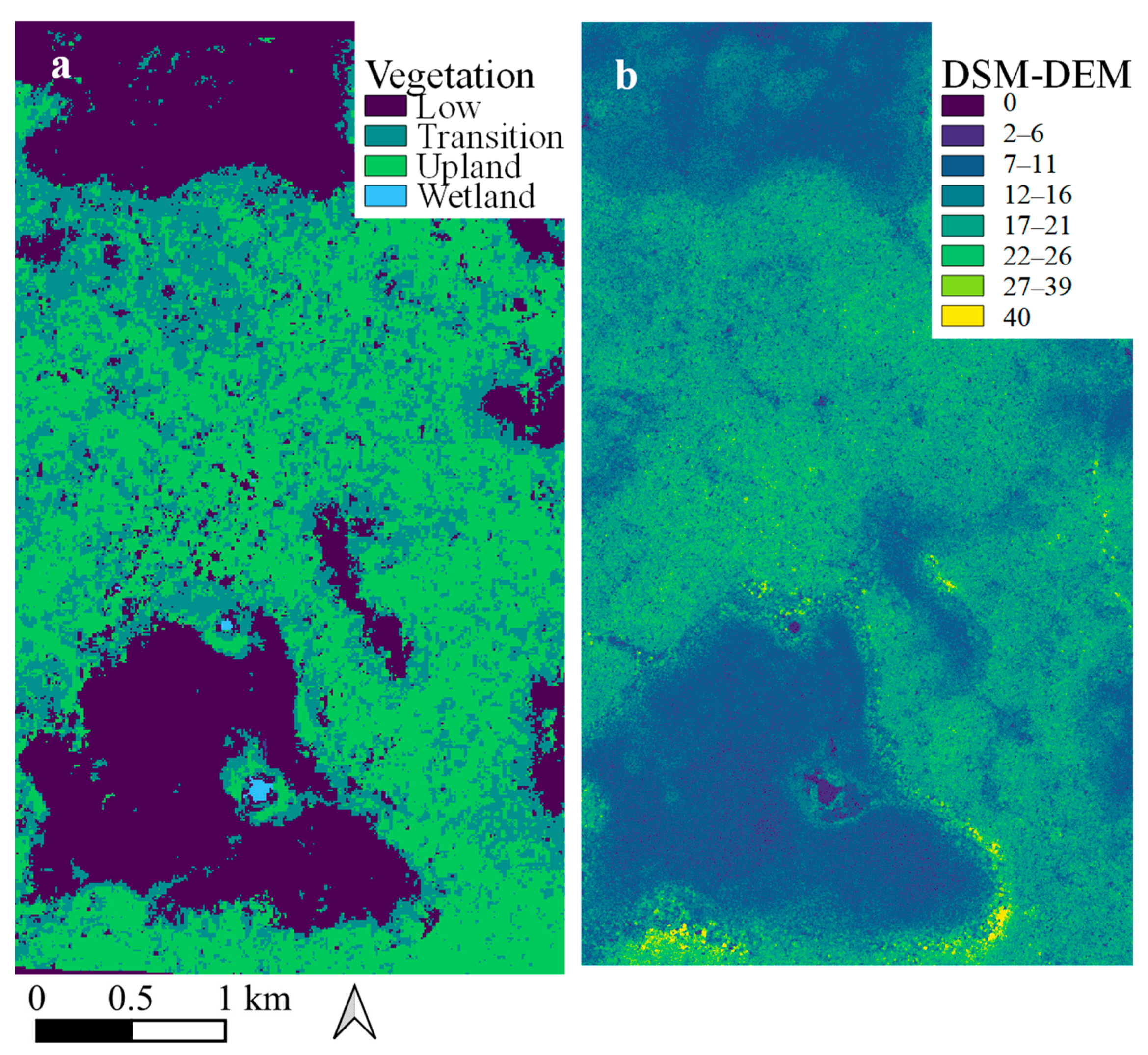
2.2. Vegetation Classification
2.3. Forest Survey Transects
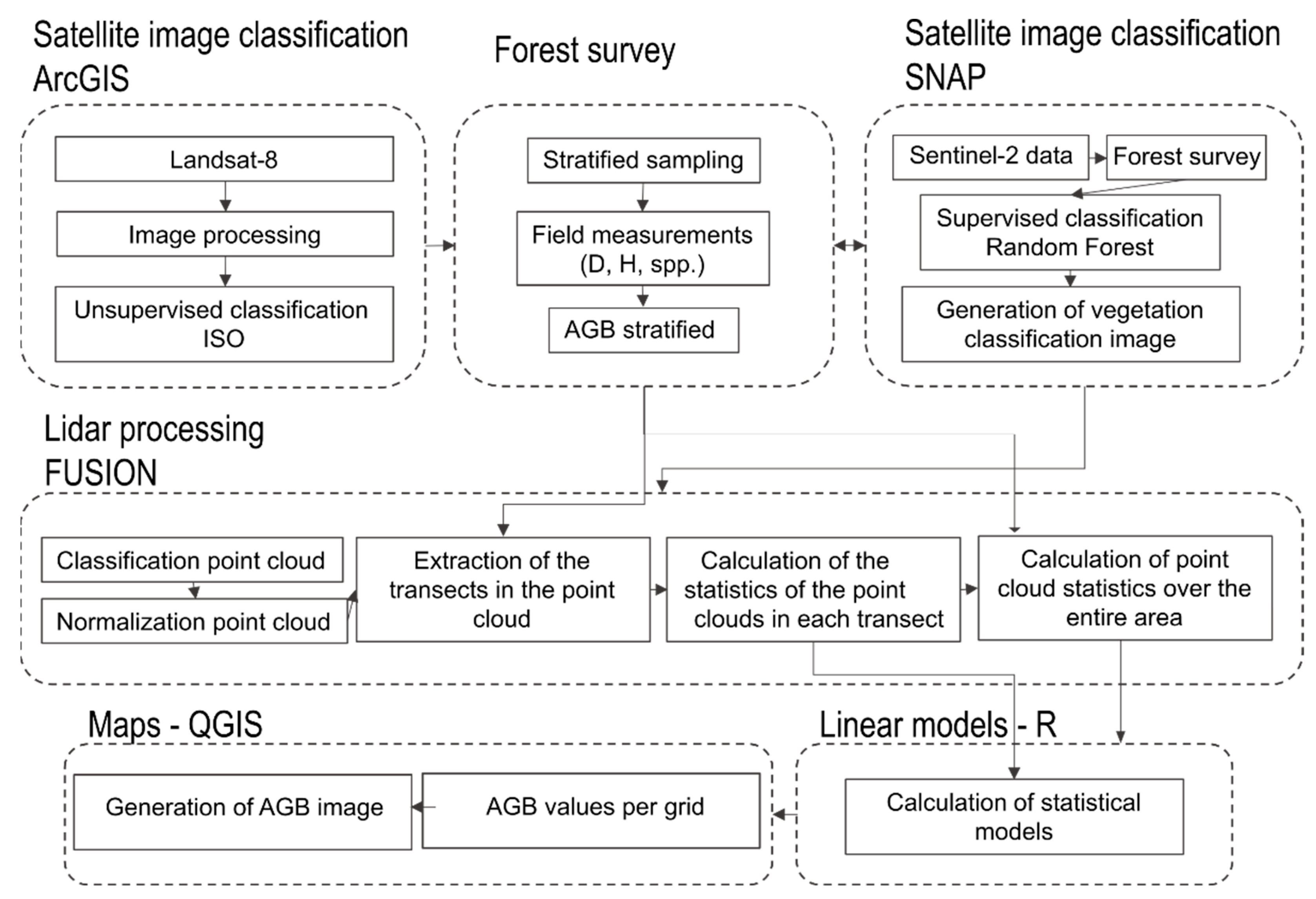
2.4. Lidar Aboveground Biomass Estimation
2.4.1. Lidar Data Processing
2.4.2. Linear Models
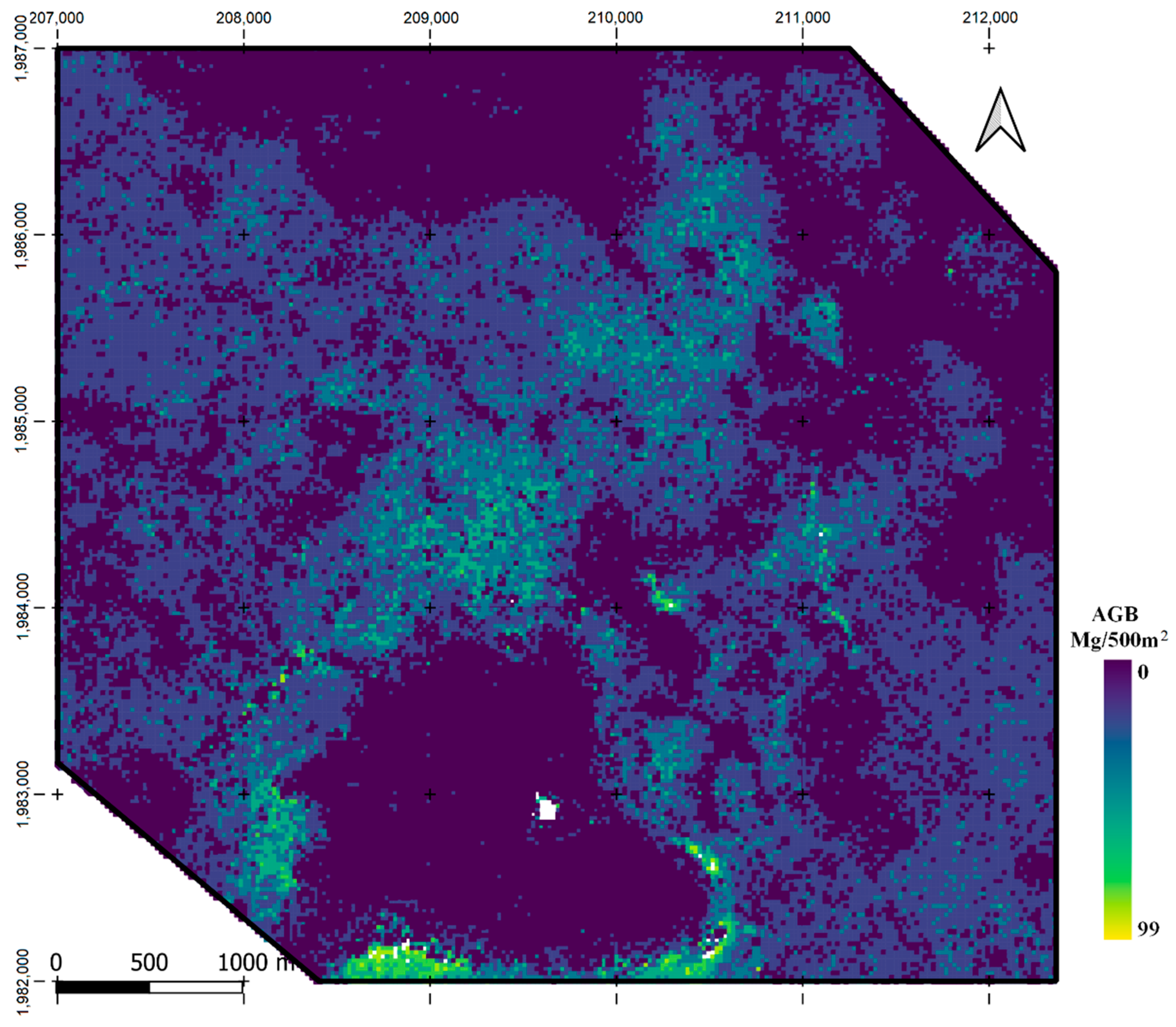
2.4.3. GIS Mapping
2.5. Forest Area Affected by Settlements
3. Results
3.1. Landscape Vegetation Communities
3.2. Forest Composition
3.3. Aboveground Biomass Estimation
3.3.1. Forest Survey AGB Estimation
3.3.2. Lidar AGB Estimation
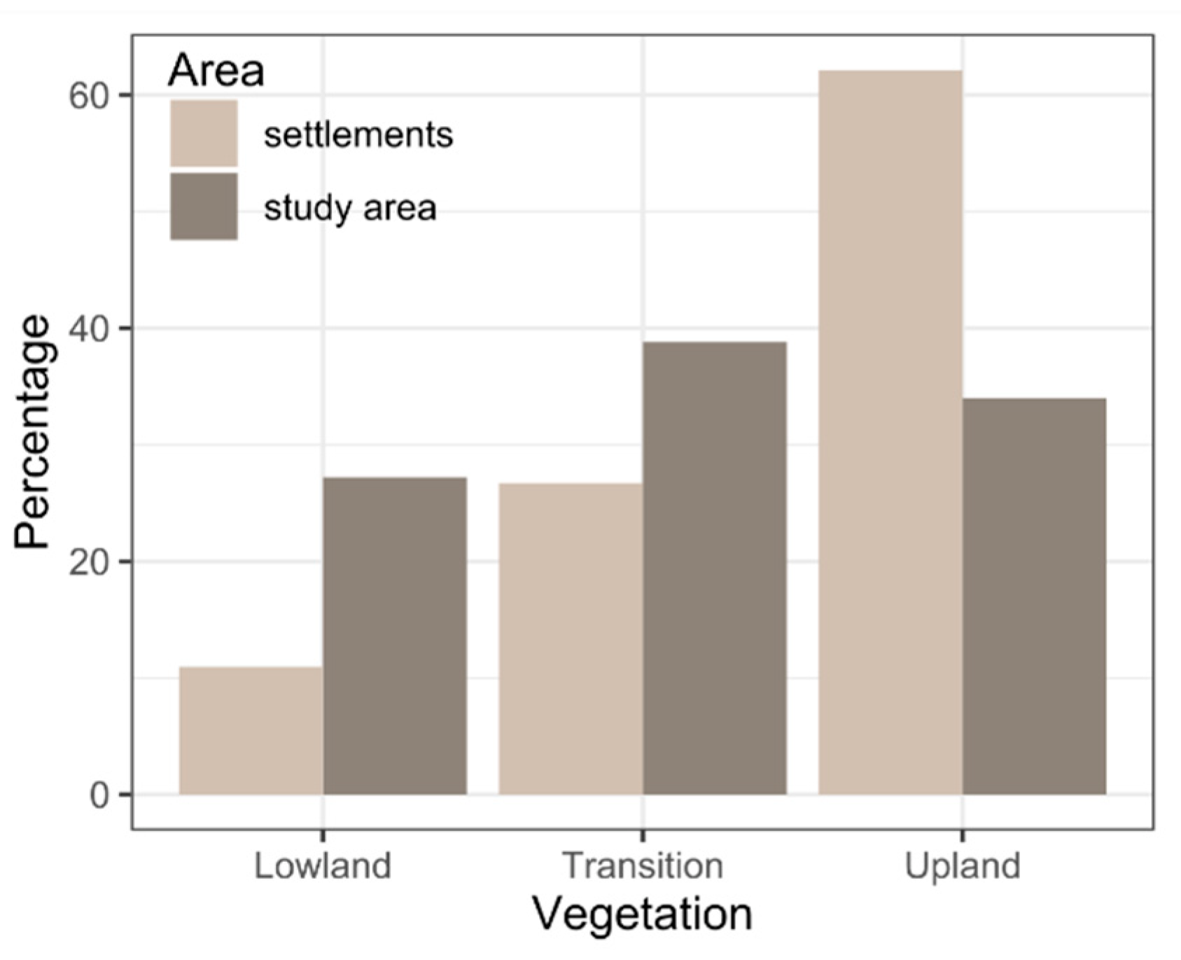
3.4. Forest Area Affected by Settlements
4. Discussion
5. Conclusions
Supplementary Materials
Author Contributions
Funding
Data Availability Statement
Acknowledgments
Conflicts of Interest
Appendix A
Appendix B

| Low Forest Species | Trees/km2 | Transition Forest Species | Trees/km2 | Upland Forest Species | Trees/km2 |
|---|---|---|---|---|---|
| Eugenia winzerlingii Standl. | 29,238 | Pouteria reticulata (Engl.) Eyma | 31,778 | Pouteria reticulata | 25,667 |
| Metopium brownei (Jacq.) Urb. | 20,190 | Drypetes lateriflora (Sw.) Krug & Urb. | 7333 | Trichilia minutiflora | 15,583 |
| Haematoxylum campechianum L. | 13,619 | Manilkara zapota (L.) P.Royen | 6667 | Brosimum alicastrum | 13,417 |
| Hyperbaena winzerlingii Standl. | 13,619 | Lonchocarpus xuul Lundell | 5630 | Drypetes lateriflora | 7083 |
| Cameraria latifolia L. | 12,476 | Nectandra coriacea (Sw.) Griseb. | 5037 | Melicoccus oliviformis Kunth | 3833 |
| Haematoxylum calakmulense | 8381 | Krugiodendron ferreum (Vahl) Urb. | 3111 | Manilkara zapota | 2667 |
| Gymnopodium floribundum Rolfe | 7429 | Brosimum alicastrum Sw. | 3037 | Protium copal (Schltdl. & Cham.) Engl. | 1583 |
| Croton arboreus Millsp. | 7333 | Gymnopodium floribundum | 3037 | Mosannona depressa (Baill.) Chatrou | 1583 |
| Erythroxylum areolatum L. | 6952 | Lonchocarpus guatemalensis Benth. | 2519 | Lonchocarpus xuul | 1167 |
| Eugenia aeruginea DC. | 5619 | Trichilia minutiflora Standl. | 2370 | Dendropanax arboreus (L.) Decne. & Planch. | 1167 |
Appendix C
| Low Vegetation | Transition Vegetation | Upland Vegetation | ||||||
|---|---|---|---|---|---|---|---|---|
| Transect | Field Mg ha−1 | Lidar Mg ha−1 | Transect | Field Mg ha−1 | Lidar Mg ha−1 | Transect | Field Mg ha−1 | Lidar Mg ha−1 |
| 18 | 3.33 | 3.37 | 01 | 8.03 | 8.97 | 05 | 22.88 | 21.90 |
| 19 | 3.49 | 3.93 | 02 | 8.28 | 8.00 | 06 | 13.59 | 13.54 |
| 20 | 5.92 | 5.43 | 03 | 16.41 | 8.37 | 07 | 22.13 | 17.43 |
| 21 | 3.91 | 4.60 | 04 | 19.53 | 14.09 | 08 | 7.83 | 7.72 |
| 31 | 5.07 | 4.76 | 11 | 14.67 | 11.45 | 09 | 9.50 | 9.12 |
| 32 | 4.56 | 3.69 | 12 | 15.08 | 11.98 | 10 | 11.83 | 9.88 |
| 33 | 2.91 | 3.69 | 13 | 9.84 | 12.29 | 22 | 20.28 | 11.70 |
| 34 | 5.67 | 4.07 | 14 | 7.72 | 12.10 | 23 | 7.31 | 12.35 |
| 35 | 1.05 | 1.79 | 15 | 11.92 | 10.85 | 24 | 12.99 | 9.94 |
| 36 | 4.00 | 3.53 | 16 | 5.73 | 7.04 | 25 | 6.13 | 6.29 |
| 37 | 3.80 | 4.72 | 17 | 6.41 | 8.64 | 26 | 3.71 | 4.95 |
| 38 | 4.58 | 4.56 | 28 | 11.05 | 6.31 | 27 | 4.28 | 4.20 |
| 39 | 3.52 | 3.95 | 46 | 10.01 | 9.08 | 29 | 5.71 | 6.28 |
| 40 | 6.44 | 5.68 | 47 | 10.34 | 10.03 | 30 | 4.73 | 5.11 |
| 41 | 4.11 | 4.84 | 48 | 8.24 | 11.30 | 56 | 12.87 | 13.76 |
| 42 | 3.34 | 4.11 | 49 | 8.81 | 10.99 | 61 | 9.42 | 9.63 |
| 43 | 3.58 | 2.90 | 50 | 17.60 | 14.58 | 62 | 8.61 | 10.76 |
| 44 | 3.29 | 2.76 | 51 | 10.86 | 11.50 | 64 | 9.84 | 8.75 |
| 45 | 2.56 | 3.32 | 52 | 11.14 | 10.02 | 65 | 11.55 | 11.48 |
| 59 | 4.15 | 3.21 | 53 | 5.06 | 11.05 | 66 | 9.25 | 14.22 |
| 63 | 4.78 | 5.14 | 54 | 10.44 | 11.35 | 67 | 10.24 | 14.18 |
| 55 | 6.06 | 8.51 | 68 | 14.52 | 12.39 | |||
| 60 | 4.90 | 6.05 | 75 | 12.06 | 16.42 | |||
| 70 | 5.30 | 7.76 | ||||||
| 71 | 11.26 | 8.35 | ||||||
| 72 | 5.70 | 6.90 | ||||||
| 74 | 4.94 | 8.70 | ||||||
| Mean | 4.00 | 4.00 | 9.83 | 9.86 | 10.92 | 10.96 | ||
| Total | 84.03 | 84.03 | 265.36 | 266.28 | 251.26 | 252.00 | ||
References
- Zhang, W.; Zhao, L.; Li, Y.; Shi, J.; Yan, M.; Ji, Y. Forest Above-Ground Biomass Inversion Using Optical and SAR Images Based on a Multi-Step Feature Optimized Inversion Model. Remote Sens. 2022, 14, 1608. [Google Scholar] [CrossRef]
- Gibbs, H.K.; Brown, S.; Niles, J.O.; Foley, J.A. Monitoring and Estimating Tropical Forest Carbon Stocks: Making REDD a Reality. Environ. Res. Lett. 2007, 2, 045023. [Google Scholar] [CrossRef]
- Li, Y.; Li, M.; Li, C.; Liu, Z. Forest Aboveground Biomass Estimation Using Landsat 8 and Sentinel-1A Data with Machine Learning Algorithms. Sci. Rep. 2020, 10, 9952. [Google Scholar] [CrossRef]
- Moradi, F.; Darvishsefat, A.A.; Pourrahmati, M.R.; Deljouei, A.; Borz, S.A. Estimating Aboveground Biomass in Dense Hyrcanian Forests by the Use of Sentinel-2 Data. Forests 2022, 13, 104. [Google Scholar] [CrossRef]
- D’Oliveira, M.V.N.; Broadbent, E.N.; Oliveira, L.C.; Almeida, D.R.A.; Papa, D.A.; Ferreira, M.E.; Zambrano, A.M.A.; Silva, C.A.; Avino, F.S.; Prata, G.A.; et al. Aboveground Biomass Estimation in Amazonian Tropical Forests: A Comparison of Aircraft- and GatorEye UAV-Borne LiDAR Data in the Chico Mendes Extractive Reserve in Acre, Brazil. Remote Sens. 2020, 12, 1754. [Google Scholar] [CrossRef]
- Rosette, J.; Surez, J.; Nelson, R.; Los, S.; Cook, B.; North, P. Lidar Remote Sensing for Biomass Assessment. In Remote Sensing of Biomass—Principles and Applications; Fatoyinbo, L., Ed.; InTech: London, UK, 2012; ISBN 978-953-51-0313-4. [Google Scholar]
- D’Oliveira, M.V.N.; Reutebuch, S.E.; McGaughey, R.J.; Andersen, H.-E. Estimating Forest Biomass and Identifying Low-Intensity Logging Areas Using Airborne Scanning Lidar in Antimary State Forest, Acre State, Western Brazilian Amazon. Remote Sens. Environ. 2012, 124, 479–491. [Google Scholar] [CrossRef]
- Clark, M.L.; Roberts, D.A.; Ewel, J.J.; Clark, D.B. Estimation of Tropical Rain Forest Aboveground Biomass with Small-Footprint Lidar and Hyperspectral Sensors. Remote Sens. Environ. 2011, 115, 2931–2942. [Google Scholar] [CrossRef]
- Phillips, O.L.; Sullivan, M.J.P.; Baker, T.R.; Monteagudo Mendoza, A.; Vargas, P.N.; Vásquez, R. Species Matter: Wood Density Influences Tropical Forest Biomass at Multiple Scales. Surv. Geophys. 2019, 40, 913–935. [Google Scholar] [CrossRef] [Green Version]
- Garrison, T.G.; Houston, S.; Alcover Firpi, O. Recentering the Rural: Lidar and Articulated Landscapes among the Maya. J. Anthropol. Archaeol. 2019, 53, 133–146. [Google Scholar] [CrossRef]
- Golden, C.; Murtha, T.; Cook, B.; Shaffer, D.S.; Schroder, W.; Hermitt, E.J.; Alcover Firpi, O.; Scherer, A.K. Reanalyzing Environmental Lidar Data for Archaeology: Mesoamerican Applications and Implications. J. Archaeol. Sci. Rep. 2016, 9, 293–308. [Google Scholar] [CrossRef] [Green Version]
- Canuto, M.A.; Estrada-Belli, F.; Garrison, T.G.; Houston, S.D.; Acuña, M.J.; Kováč, M.; Marken, D.; Nondédéo, P.; Auld-Thomas, L.; Castanet, C.; et al. Ancient Lowland Maya Complexity as Revealed by Airborne Laser Scanning of Northern Guatemala. Science 2018, 361, eaau0137. [Google Scholar] [CrossRef] [PubMed] [Green Version]
- Lentz, D.L.; Magee, K.; Weaver, E.; Jones, J.G.; Tankersley, K.B.; Hood, A.; Islebe, G.; Hernandez, C.E.R.; Dunning, N.P. Agroforestry and Agricultural Practices of the Ancient Maya at Tikal. In Tikal: Paleoecology of an Ancient Maya City; Cambridge University Press: Cambridge, UK, 2015; pp. 152–185. [Google Scholar]
- Lentz, D.L.; Dunning, N.P.; Scarborough, V.L.; Magee, K.S.; Thompson, K.M.; Weaver, E.; Carr, C.; Terry, R.E.; Islebe, G.; Tankersley, K.B.; et al. Forests, Fields, and the Edge of Sustainability at the Ancient Maya City of Tikal. Proc. Natl. Acad. Sci. USA 2014, 111, 18513–18518. [Google Scholar] [CrossRef] [PubMed] [Green Version]
- Dunning, N.P.; Anaya Hernández, A.; Beach, T.; Carr, C.; Griffin, R.; Jones, J.G.; Lentz, D.L.; Luzzadder-Beach, S.; Reese-Taylor, K.; Šprajc, I. Margin for Error: Anthropogenic Geomorphology of Bajo Edges in the Maya Lowlands. Geomorphology 2019, 331, 127–145. [Google Scholar] [CrossRef]
- Reese-Taylor, K. Founding Landscapes in the Central Karstic Uplands. In Maya E Groups: Calendars, Astronomy, and Urbanism in the Early Lowlands; University Press of Florida: Gainesville, FL, USA, 2017; pp. 480–514. ISBN 978-0-8130-5435-3. [Google Scholar]
- Thompson, K.M.; Hood, A.; Cavallaro, D.; Lentz, D.L. Connecting Contemporary Ecology and Ethnobotany to Ancient Plant Use Practices of the Maya at Tikal. In Tikal: Paleoecology of an Ancient Maya City; Lentz, D.L., Dunning, N.P., Scarborough, V.L., Eds.; Cambridge University Press: Cambridge, UK, 2015; pp. 124–151. ISBN 978-1-107-02793-0. [Google Scholar]
- CONAGUA Servicio Meteorológico Nacional. Available online: https://smn.conagua.gob.mx/es/ (accessed on 25 January 2022).
- Holdridge, L.R.; Grenke, W.C.; Hatheway, W.H.; Liang, T.; Tosi, J.J.A.; WNRE INC CHESTERTOWN MD. Forest Environments in Tropical Life Zones. A Pilot Study; Defense Technical Information Center: Fort Belvoir, VA, USA, 1971; ISBN 978-0-08-016340-6. [Google Scholar]
- Pennington, T.D.; Sarukhán, J. Arboles Tropicales de México; Universidad Nacional Autónoma de México: Mexico City, Mexico, 2005. [Google Scholar]
- Miranda, F.; Hernández-X, E. Los Tipos de Vegetación de México y su Clasificación: Edición Conmemorativa 1963–2013; Ediciones Científicas Universitarias Serie texto Científico Universitario; Sociedad Botánica de México: Mexico City, Mexico, 2015; ISBN 978-607-16-1863-4. [Google Scholar]
- Martínez, E.; Sousa, M.; Ramos, C. Región de Calakmul, Campeche; Listados florísticos de México; Universidad Nacional Autónoma de México: Mexico, Mexico, 2001. [Google Scholar]
- Martínez, E.; Galindo-Leal, C. La Vegetación de Calakmul, Campeche, México: Clasificación, Descripción y Distribución. Bot. Sci. 2002, 71, 7–32. [Google Scholar] [CrossRef]
- Reese-Taylor, K.; Hernández, A.A.; Esquivel, F.C.A.F.; Monteleone, K.; Uriarte, A.; Carr, C.; Acuña, H.G.; Fernandez-Diaz, J.C.; Peuramaki-Brown, M.; Dunning, N. Boots on the Ground at Yaxnohcah: Ground-Truthing Lidar in a Complex Tropical Landscape. Adv. Archaeol. Pract. 2016, 4, 314–338. [Google Scholar] [CrossRef]
- Carr, C. Clasificación de Comunidades de Vegetación En Yaxnohcah Mediante La Utilización de Imágenes Satelitales de Landsat. In Proyecto Arqueológico Yaxnohcah, Informe de la 2016 Temporada de Investigaciones; Instituto Nacional de Antropología e Historia: Mexico City, Mexico, 2017. [Google Scholar]
- ESA. Sentinel Applications Platform; European Space Agency: Paris, France, 2022. [Google Scholar]
- Chave, J.; Réjou-Méchain, M.; Búrquez, A.; Chidumayo, E.; Colgan, M.S.; Delitti, W.B.C.; Duque, A.; Eid, T.; Fearnside, P.M.; Goodman, R.C.; et al. Improved Allometric Models to Estimate the Aboveground Biomass of Tropical Trees. Glob. Change Biol. 2015, 20, 3177–3190. [Google Scholar] [CrossRef]
- Zanne, A.E.; Lopez-Gonzalez, G.; Coomes, D.A.; Ilic, J.; Jansen, S.; Lewis, S.L.; Miller, R.B.; Swenson, N.G.; Wiemann, M.C.; Chave, J. Data from: Towards a Worldwide Wood Economics Spectrum. Ecol. Lett. 2009, 12, 351–366. [Google Scholar]
- Sullivan, M.J.P.; Talbot, J.; Lewis, S.L.; Phillips, O.L.; Qie, L.; Begne, S.K.; Chave, J.; Cuni-Sanchez, A.; Hubau, W.; Lopez-Gonzalez, G.; et al. Diversity and Carbon Storage across the Tropical Forest Biome. Sci. Rep. 2017, 7, 39102. [Google Scholar] [CrossRef] [Green Version]
- R Core Team. R: The R Project for Statistical Computing; The R Foundation: Vienna, Austria, 2022. [Google Scholar]
- Réjou-Méchain, M.; Tanguy, A.; Piponiot, C.; Chave, J.; Hérault, B. BIOMASS: An r Package for Estimating Above-ground Biomass and Its Uncertainty in Tropical Forests. Methods Ecol. Evol. 2017, 8, 1163–1167. [Google Scholar] [CrossRef]
- Bettinger, P.; Boston, K.; Siry, J.P.; Grebner, D.L. Valuing and Characterizing Forest Conditions. In Forest Management and Planning; Elsevier: London, UK, 2017; pp. 21–63. ISBN 978-0-12-809476-1. [Google Scholar]
- Slik, J.W.F.; Aiba, S.-I.; Brearley, F.Q.; Cannon, C.H.; Forshed, O.; Kitayama, K.; Nagamasu, H.; Nilus, R.; Payne, J.; Paoli, G.; et al. Environmental Correlates of Tree Biomass, Basal Area, Wood Specific Gravity and Stem Density Gradients in Borneo’s Tropical Forests. Glob. Ecol. Biogeogr. 2010, 19, 50–60. [Google Scholar] [CrossRef]
- Global Mapper Pro; Blue Marble Geographics: Hallowell, ME, USA, 2022.
- McGaughey, R.J. FUSION/LDV: Software for LIDAR Analysis and Visualization. Version 4.21; United States Department of Agriculture, Forest Service, Pacific Northwest Research Station: Portland, OR, USA, 2021.
- Fox, J.; Bouchet-Valat, M. Rcmdr-Package: R Commander; Chapman and Hall/CRC Press: Boca Raton, FL, USA, 2020. [Google Scholar]
- QGIS Geographic Information System; QGIS Association. 2022. Available online: https://qgis.org/en/site/ (accessed on 5 June 2022).
- Anaya Hernández, A.; Reese-Taylor, K. (Eds.) Proyecto Arqueológico Yaxnohcah. Informe de Las Temporadas de Investigación 2016; University of Calgary: Calgary, AB, Canada, 2017. [Google Scholar]
- Vázquez López, V.A.; Anaya Hernández, A.; Reese-Taylor, K. (Eds.) Proyecto Arqueológico Yaxnohcah. Informe de Las Temporadas de Investigación 2017–2018; University of Calgary: Calgary, AB, Canada, 2019. [Google Scholar]
- Read, L.; Lawrence, D. Recovery of Biomass Following Shifting Cultivation in Dry Tropical Forests of the Yucatan. Ecol. Appl. 2003, 13, 85–97. [Google Scholar] [CrossRef] [Green Version]
- Cairns, M.A.; Olmsted, I.; Granados, J.; Argaez, J. Composition and Aboveground Tree Biomass of a Dry Semi-Evergreen Forest on Mexico’s Yucatan Peninsula. For. Ecol. Manag. 2003, 186, 125–132. [Google Scholar] [CrossRef]
- NASA NASA JPL. Global Above Ground Biomass Mean Prediction. 2020. Available online: Earthdata.nasa.gov (accessed on 8 February 2022).
- Ortiz-Reyes, A.D.; Valdez-Lazalde, J.R.; Ángeles-Pérez, G.; los Santos-Posadas, H.M.D.; Schneider, L.; Aguirre-Salado, C.A.; Peduzzi, A. Transectos de datos LiDAR: Una estrategia de muestreo para estimar biomasa aérea en áreas forestales. Madera Y Bosques 2019, 25, e2531872. [Google Scholar] [CrossRef] [Green Version]
- Puc-Kauil, R.; Ángeles-Pérez, G.; Valdez-Lazalde, J.R.; Reyes-Hernández, V.J.; Dupuy-Rada, J.M.; Schneider, L.; Pérez-Rodríguez, P.; García-Cuevas, X. Species-Specific Biomass Equations for Small-Size Tree Species in Secondary Tropical Forests. Trop. Subtrop. Agroecosystems 2019, 22, 735–754. [Google Scholar]
- Lundell, C. Preliminary Sketch of the Phytogeography of the Yucatan Peninsula; Carnegie Institute of Washington: Washington, DC, USA, 1934. [Google Scholar]
- Lentz, D.L.; Hamilton, T.L.; Dunning, N.P.; Jones, J.G.; Reese-Taylor, K.; Anaya Hernández, A.; Walker, D.S.; Tepe, E.J.; Carr, C.; Brewer, J.L.; et al. Paleoecological Studies at the Ancient Maya Center of Yaxnohcah Using Analyses of Pollen, Environmental DNA, and Plant Macroremains. Front. Ecol. Evol. 2022, 10, 445. [Google Scholar] [CrossRef]
- Kabukcu, C. Wood Charcoal Analysis in Archaeology. In Environmental Archaeology: Current Theoretical and Methodological Approaches; Pişkin, E., Marciniak, A., Bartkowiak, M., Eds.; Interdisciplinary Contributions to Archaeology; Springer International Publishing: Cham, Switzerland, 2018; pp. 133–154. ISBN 978-3-319-75082-8. [Google Scholar]
- Hernández-Montejo, C. Del Palo de Tinte al Camarón; Gobierno del Estado de Campeche, Instituto de Cultura, Instituto de Antropología e Historia, Universidad Autónoma de Campeche: Campeche, Mexico, 2005. [Google Scholar]
- Bauer-Gottwein, P.; Gondwe, B.R.N.; Charvet, G.; Marín, L.E.; Rebolledo-Vieyra, M.; Merediz-Alonso, G. Review: The Yucatán Peninsula Karst Aquifer, Mexico. Hydrogeol. J. 2011, 19, 507–524. [Google Scholar] [CrossRef]
- Prümers, H.; Betancourt, C.J.; Iriarte, J.; Robinson, M.; Schaich, M. Lidar Reveals Pre-Hispanic Low-Density Urbanism in the Bolivian Amazon. Nature 2022, 606, 325–328. [Google Scholar] [CrossRef]
- Brewer, J.L.; Carr, C. Household Quarry-Reservoirs at the Ancient Maya Site of Yaxnohcah, Mexico. Lat. Am. Antiq. 2021, 33, 432–440. [Google Scholar] [CrossRef]


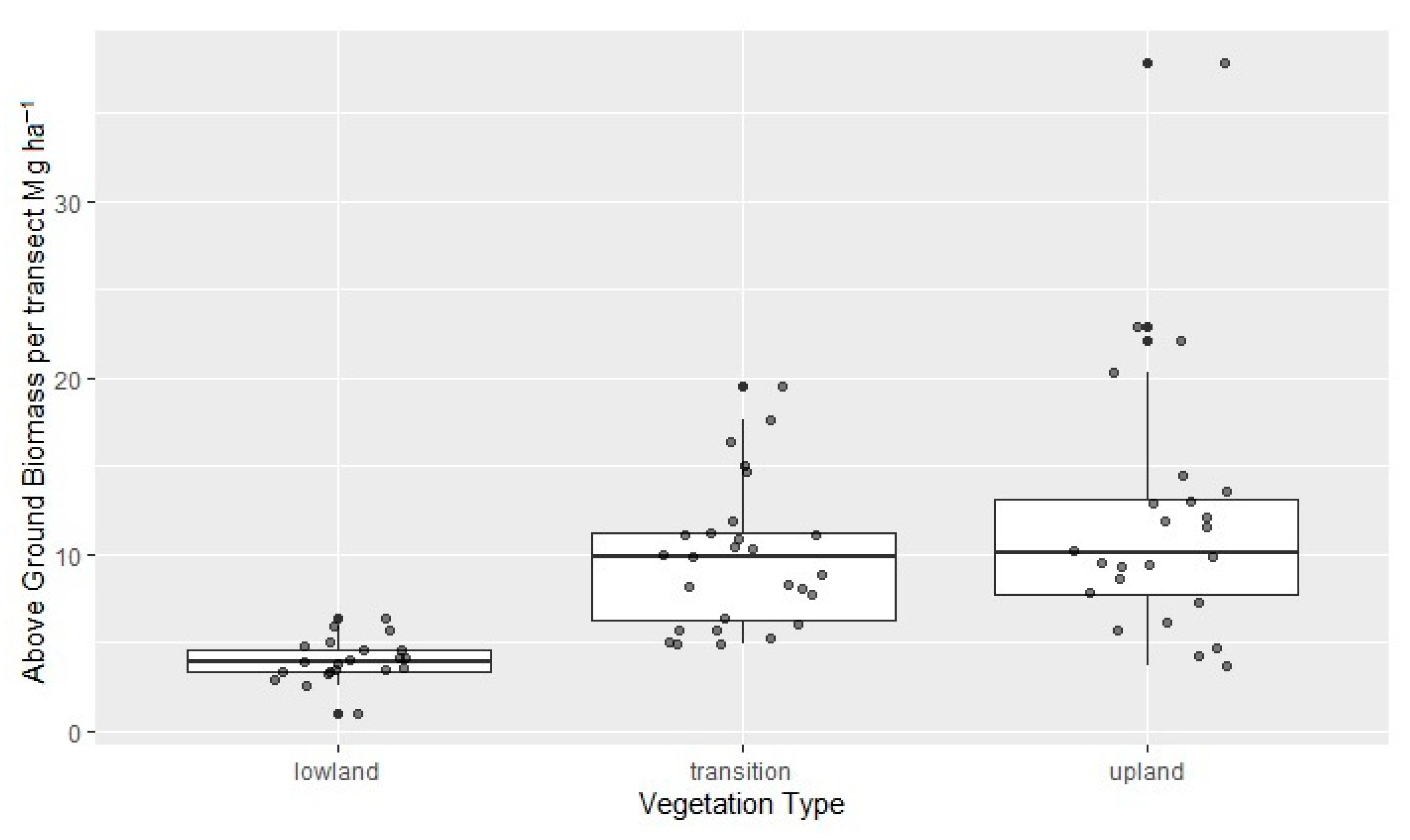
| Vegetation Type | No. Transects | Ha | Basal Area m2 ha−1 | Sum of AGB | AGB Mg ha−1 | AGC Mg ha−1 |
|---|---|---|---|---|---|---|
| Lowland | 21 | 1.05 | 17.85 | 84.03 | 80.03 | 37.70 |
| Transition | 27 | 1.35 | 25.19 | 265.36 | 196.57 | 92.58 |
| Upland | 24 | 1.20 | 29.08 | 289.05 | 240.88 | 113.45 |
| Vegetation Type | Linear Model | F | Adj. R2 | RSE |
|---|---|---|---|---|
| Low | AGB ~ 2.323 + 6.653 × MAD mode + −4.645 × AAD | 15.18 | 0.59 | 0.77 |
| Transition | AGB ~ 0.157 × exp(0.077 × “P95”) × “AAD” ^ 0.333 × 1.062 | 5.92 | 0.27 | 0.35 |
| Upland | AGB ~ 0.442 × exp(0.514 × “P80”) × exp(−0.298 × “P90”) × 1.033 | 30.58 | 0.73 | 0.25 |
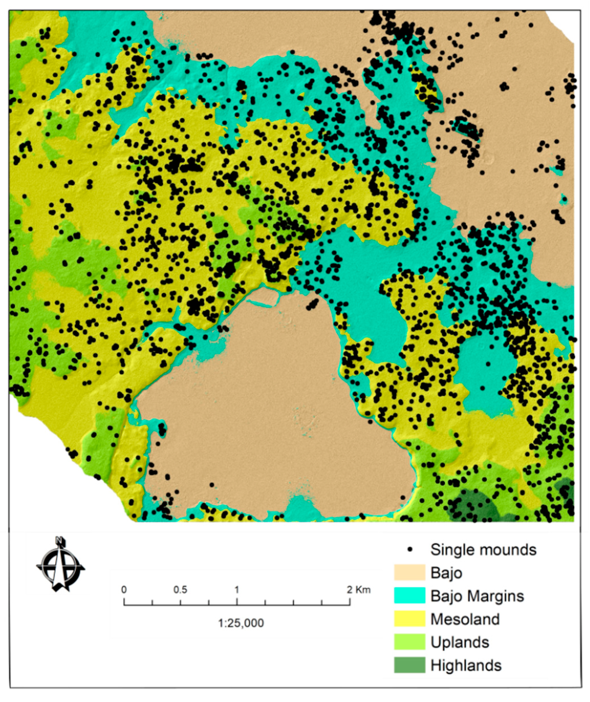
| Topo Zone | Elevation (masl) | f_Mounds | f % | Area (ha) | Area % | Density/ha |
|---|---|---|---|---|---|---|
| Bajo | 219.49–232.87 | 292 | 8.12 | 1789.31 | 33.24 | 0.37 |
| Bajo Margins | 232.87–243.34 | 849 | 23.61 | 866.09 | 16.09 | 1.28 |
| Mesoland | 243.34–252.59 | 1502 | 41.77 | 1195.37 | 22.21 | 1.43 |
| Upland | 252.59–262.81 | 859 | 23.88 | 1114.15 | 20.70 | 1.58 |
| Highland | 262.81–281.54 | 94 | 2.61 | 418.28 | 7.77 | 1.83 |
| Total | 3596 | 100 | 2410.51 | 100 | 0.67 |
Publisher’s Note: MDPI stays neutral with regard to jurisdictional claims in published maps and institutional affiliations. |
© 2022 by the authors. Licensee MDPI, Basel, Switzerland. This article is an open access article distributed under the terms and conditions of the Creative Commons Attribution (CC BY) license (https://creativecommons.org/licenses/by/4.0/).
Share and Cite
Vázquez-Alonso, M.; Lentz, D.L.; Dunning, N.P.; Carr, C.; Anaya Hernández, A.; Reese-Taylor, K. Lidar-Based Aboveground Biomass Estimations for the Maya Archaeological Site of Yaxnohcah, Campeche, Mexico. Remote Sens. 2022, 14, 3432. https://doi.org/10.3390/rs14143432
Vázquez-Alonso M, Lentz DL, Dunning NP, Carr C, Anaya Hernández A, Reese-Taylor K. Lidar-Based Aboveground Biomass Estimations for the Maya Archaeological Site of Yaxnohcah, Campeche, Mexico. Remote Sensing. 2022; 14(14):3432. https://doi.org/10.3390/rs14143432
Chicago/Turabian StyleVázquez-Alonso, Mariana, David L. Lentz, Nicholas P. Dunning, Christopher Carr, Armando Anaya Hernández, and Kathryn Reese-Taylor. 2022. "Lidar-Based Aboveground Biomass Estimations for the Maya Archaeological Site of Yaxnohcah, Campeche, Mexico" Remote Sensing 14, no. 14: 3432. https://doi.org/10.3390/rs14143432
APA StyleVázquez-Alonso, M., Lentz, D. L., Dunning, N. P., Carr, C., Anaya Hernández, A., & Reese-Taylor, K. (2022). Lidar-Based Aboveground Biomass Estimations for the Maya Archaeological Site of Yaxnohcah, Campeche, Mexico. Remote Sensing, 14(14), 3432. https://doi.org/10.3390/rs14143432