
Spatiotemporal Modeling of Zoonotic Arbovirus Transmission in Northeastern Florida Using Sentinel Chicken Surveillance and Earth Observation Data

 , , ,
, , , 

Abstract
:
1. Introduction
2. Materials and Methods
2.1. Land Cover Data
2.2. Climate Data
2.3. Variable Reduction
2.4. Candidate Sets and Model Runs
2.5. Bayesian Modeling
3. Results
4. Discussion
5. Conclusions
Supplementary Materials
Author Contributions
Funding
Data Availability Statement
Acknowledgments
Conflicts of Interest
References
- World Health Organization. World Health Organization. World health statistics. In World Health Organization Report; World Health Organization: Geneva, Switzerland, 2013. [Google Scholar]
- World Health Organization. Manual on Environmental Management for Mosquito Control, with Special Emphasis on Malaria Vectors; World Health Organization: Geneva, Switzerland, 1982. [Google Scholar]
- Kalluri, S.; Gilruth, P.; Rogers, D.; Szczur, M. Surveillance of Arthropod Vector-Borne Infectious Diseases Using Remote Sensing Techniques: A Review. PLOS Pathog. 2007, 3, e116. [Google Scholar] [CrossRef] [PubMed]
- Kitron, U. Landscape Ecology and Epidemiology of Vector-Borne Diseases: Tools for Spatial Analysis. J. Med. Èntomol. 1998, 35, 435–445. [Google Scholar] [CrossRef] [PubMed]
- Banerjee, S.; Carlin, B.P.; Gelfand, A.E. Hierarchical Modeling and Analysis for Spatial Data; Chapman & Hall/CRC: Boca Raton, FL, USA, 2004. [Google Scholar]
- Lindsey, N.P.; Lehman, J.A.; Staples, J.E.; Fisher, M. West Nile virus and other nationally notifiable arboviral diseases–United States. MMWR Morb. Mortal. Wkly. Rep. 2014, 64, 929–934. [Google Scholar] [CrossRef] [Green Version]
- Scott, T.W.; Weaver, S.C. Eastern Equine Encephalomyelitis Virus: Epidemiology and Evolution of Mosquito Transmission. In Advances in Virus Research; Maramorosch, K., Murphy, F.A., Shatkin, A.J., Eds.; Academic Press: Cambridge, MA, USA, 1989; pp. 277–328. [Google Scholar]
- Reisen, W.K. Ecology of West Nile Virus in North America. Viruses 2013, 5, 2079–2105. [Google Scholar] [CrossRef] [PubMed]
- Wisely, S.W.; Hood, K. Fact Sheet: Eastern Equine Encephalitis. In Electronic Data Information Source; University of Florida: Gainesville, FL, USA, 2019. [Google Scholar] [CrossRef]
- American Association Equine Practitioners. Infectious Disease Guidelines: West Nile Virus [Fact Sheet]; American Association Equine Practitioners: Lexington, KY, USA, 2017. [Google Scholar]
- Armstrong, P.M.; Andreadis, T.G. Ecology and Epidemiology of Eastern Equine Encephalitis Virus in the Northeastern United States: An Historical Perspective. J. Med Èntomol. 2022, 59, 1–13. [Google Scholar] [CrossRef]
- Rochlin, I.; Faraji, A.; Healy, K.; Andreadis, T.G. West Nile Virus Mosquito Vectors in North America. J. Med Èntomol. 2019, 56, 1475–1490. [Google Scholar] [CrossRef]
- Day, J.F.; Tabachnick, W.J.; Smartt, C.T. Factors That Influence the Transmission of West Nile Virus in Florida. J. Med. Entomol. 2015, 52, 743–754. [Google Scholar] [CrossRef]
- Day, J.F.; Shaman, J. Mosquito-borne arboviral surveillance and the prediction of disease outbreaks. In Flavivirus Encephalitis; Ruzek, D., Ed.; InTech: Rijeka, Croatia, 2011; pp. 105–130. [Google Scholar]
- Kelen, P.T.V.; A Downs, J.; Stark, L.M.; Loraamm, R.W.; Anderson, J.H.; Unnasch, T.R. Spatial epidemiology of eastern equine encephalitis in Florida. Int. J. Health Geogr. 2012, 11, 47. [Google Scholar] [CrossRef] [Green Version]
- Kelen, P.V.; Downs, J.A.; Unnasch, T.; Stark, L. A risk index model for predicting eastern equine encephalitis virus transmission to horses in Florida. Appl. Geogr. 2014, 48, 79–86. [Google Scholar] [CrossRef] [Green Version]
- Sallam, M.F.; Xue, R.-D.; Pereira, R.M.R.; Koehler, P.G. Ecological niche modeling of mosquito vectors of West Nile virus in St. John’s County, Florida, USA. Parasites Vectors 2016, 9, 371. [Google Scholar] [CrossRef]
- Burch, C.; Loraamm, R.; Unnasch, T.; Downs, J. Utilizing ecological niche modelling to predict habitat suitability of eastern equine encephalitis in Florida. Ann. GIS 2020, 26, 133–147. [Google Scholar] [CrossRef] [Green Version]
- Beeman, S.P.; Downs, J.A.; Unnasch, T.R.; Unnasch, R.S. West Nile Virus and Eastern Equine Encephalitis Virus High Probability Habitat Identification for the Selection of Sentinel Chicken Surveillance Sites in Florida. J. Am. Mosq. Control Assoc. 2022, 38, 1–6. [Google Scholar] [CrossRef] [PubMed]
- Heberlein-Larson, L.A.; Tan, Y.; Stark, L.M.; Cannons, A.C.; Shilts, M.H.; Unnasch, T.R.; Das, S.R. Complex Epidemiological Dynamics of Eastern Equine Encephalitis Virus in Florida. Am. J. Trop. Med. Hyg. 2019, 100, 1266–1274. [Google Scholar] [CrossRef] [PubMed]
- Shaman, J.; Day, J.F.; Stieglitz, M. Drought-Induced Amplification and Epidemic Transmission of West Nile Virus in Southern Florida. J. Med. Èntomol. 2005, 42, 134–141. [Google Scholar] [CrossRef] [PubMed]
- Miley, K.M.; Downs, J.; Beeman, S.P.; Unnasch, T.R. Impact of the Southern Oscillation Index, Temperature, and Precipitation on Eastern Equine Encephalitis Virus Activity in Florida. J. Med. Èntomol. 2020, 57, 1604–1613. [Google Scholar] [CrossRef] [PubMed]
- Morrison, A.; Giandomenico, D.; Stanek, D.; Heberlein-Larson, L.; Castaneda, M.; Mock, V.; Blackmore, C. Florida Arbovirus Surveillance Week 52: December 23–29; Florida Department of Health: Tallahassee, FL, USA, 2018. [Google Scholar]
- Florida Fish and Wildlife Conservation Commission and Florida Natural Areas Inventory. Cooperative Land Cover; Version 3.3; Raster: Tallahassee, FL, USA, 2021. [Google Scholar]
- Kottek, M.; Grieser, J.; Beck, C.; Rudolf, B.; Rubel, F. World map of the Köppen-Geiger climate classification updated. Meteorol. Z. 2006, 15, 259–263. [Google Scholar] [CrossRef]
- Winsberg, M.D. Florida Weather, 2nd ed.; University Press of Florida: Gainesville, FL, USA, 2003. [Google Scholar]
- Lloyd, A.; Connelly, C.; Carlson, D. Florida Mosquito Control: The State of the Mission as Defined by Mosquito Controllers, Regulators, and Environmental Managers; Florida Coordinating Council on Mosquito Control: Vero Beach, FL, USA, 2018.
- Florida Department of Health (FDOH). Non-Human Mosquito-Borne Disease Monitoring Activities; FDOH: Tampa, FL, USA, 2021.
- McGarigal, K.; Marks, B.J. Spatial pattern analysis program for quantifying landscape structure. In General Technical Report. PNW-GTR-351; US Department of Agriculture, Forest Service, Pacific Northwest Research Station: Portland, OR, USA, 1995; p. 122. [Google Scholar]
- Gergel, S.E.; Turner, M.G.; Miller, J.R.; Melack, J.M.; Stanley, E.H. Landscape indicators of human impacts to riverine systems. Aquat. Sci. 2002, 64, 118–128. [Google Scholar] [CrossRef]
- Hesselbarth, M.; Sciaini, M.; With, K.; Wiegand, K.; Nowosad, J. Landscapemetrics: An open-source R tool to calculate landscape metrics. Ecography 2019, 42, 1–10. [Google Scholar] [CrossRef] [Green Version]
- R Core Team. R: A Language and Environment for Statistical Computing; R Foundation for Statistical Computing: Vienna, Austria, 2021. [Google Scholar]
- Beven, K.J.; Kirkby, M.J. A physically based, variable contributing area model of basin hydrology/Un modèle à base physique de zone d’appel variable de l’hydrologie du bassin versant. Hydrolog. Sci. J. 1979, 24, 43–69. [Google Scholar] [CrossRef] [Green Version]
- Du, J. NCEP/EMC 4KM Gridded Data (GRIB) Stage IV Data; Version 1.0; UCAR/NCAR—Earth Observing Laboratory: Boulder, CO, USA, 2011. [Google Scholar]
- Wan, Z.; Zhang, Y.; Zhang, Q.; Li, Z.L. Validation of the land-surface temperature products retrieved from Terra Moderate Resolution Imaging Spectroradiometer data. Remote Sens. Environ. 2002, 83, 163–180. [Google Scholar] [CrossRef]
- Mullen, G.R.; Durden, L.A. Medical and Veterinary Entomology, 3rd ed.; Academic Press: Cambridge, MA, USA, 2019. [Google Scholar]
- Tuszynski, J. caTools: Tools: Moving Window Statistics, GIF, Base 64, ROC AUC, etc. R Package, Version 1.18.0.; 2020. Available online: https://cran.r-project.org/web/packages/caTools/index.html (accessed on 11 May 2022).
- Zuur, A.F.; Ieno, E.N.; Walker, N.; Saveliev, A.A.; Smith, G.M. Mixed Effects Models and Extensions in Ecology with R, 1st ed.; Springer: New York, NY, USA, 2009. [Google Scholar]
- Brooks, M.E.; Kristensen, K.; van Benthem, K.J.; Magnusson, A.; Berg, C.W.; Nielsen, A.; Skaug, H.J.; Machler, M.; Bolker, B.M. glmmTMB Balances Speed and Flexibility Among Packages for Zero-inflated Generalized Linear Mixed Modeling. R J. 2017, 9, 378–400. [Google Scholar] [CrossRef] [Green Version]
- Barton, K. MuMIn: Multi-Model Inference, R Package Version 1.43.15; 2019. Available online: https://cran.r-project.org/web/packages/MuMIn/index.html (accessed on 11 May 2022).
- Akaike, H. Information Theory and an Extension of the Maximum Likelihood Principle. In Proceedings of the 2nd International Symposium on Information Theory, Tsahkadsor, Armenia, 2–8 September 1971; Petrov, B.N., Csáki, F., Eds.; Akadémiai Kiadó: Budapest, Hungary, 1973; pp. 267–281. [Google Scholar]
- Burnham, K.P.; Anderson, D.R. Model Selection and Multimodel Inference: A Practical Information-Theoretic Approach, 2nd ed.; Springer: New York, NY, USA, 2002; ISBN 0-387-95364-7. [Google Scholar]
- Lindgren, F.; Rue, H. Bayesian Spatial Modelling with R-INLA. J. Stat. Softw. 2015, 63, 1–2. [Google Scholar] [CrossRef] [Green Version]
- Rue, R.; Martino, S.; Chopin, N. Approximate Bayesian inference for latent Gaussian models using inte-grated nested Laplace approximations (with discussion). J. R Stat. B Soc. 2009, 71, 319–392. [Google Scholar] [CrossRef]
- Zuur, A.F.; Ieno, E.N.; Saveliev, A.A. Beginner’s Guide to Spatial, Temporal, and Spatial-Temporal Ecological Data Analysis with R-INLA; Highland Statistics Ltd.: Newburgh, IN, USA, 2017; Volume 7. [Google Scholar]
- Lindgren, F.; Rue, H.; Lindström, J. An explicit link between Gaussian fields and Gaussian Markov random fields: The stochastic partial differential equation approach. J. R. Stat. Soc. Ser. B Stat. Methodol. 2011, 73, 423–498. [Google Scholar] [CrossRef] [Green Version]
- Simpson, J.E.; Schweinfest, C.W.; Shull, G.E.; Gawenis, L.R.; Walker, N.M.; Boyle, K.T.; Soleimani, M.; Clarke, L.L. PAT-1 (Slc26a6) is the predominant apical membrane Cl-/HCO3- exchanger in the upper villous epithelium of the murine duodenum. Am. J. Physiol. -Gastr. L 2007, 292, G1079–G1088. [Google Scholar] [CrossRef] [Green Version]
- Spiegelhalter, D.J.; Best, N.G.; Carlin, B.P.; van der Linde, A. Bayesian measures of model complexity and fit. J. R. Stat. Soc. Ser. B Stat. Methodol. 2002, 64, 583–616. [Google Scholar] [CrossRef] [Green Version]
- Thiele, C.; Hershfield, G. Cutpointr: Improved Estimation and Validation of Optimal Cutpoints in R. J. Stat. Softw. 2021, 98, 1–27. [Google Scholar] [CrossRef]
- Hoeting, J.A. The importance of accounting for spatial and temporal correlation in analyses of ecological data. Ecol. Appl. 2009, 19, 574–577. [Google Scholar] [CrossRef] [PubMed]
- Martínez-Beneito, M.A.; López-Quílez, A.; Rocamora, P.B. An autoregressive approach to spatio-temporal disease mapping. Stat. Med. 2008, 27, 2874–2889. [Google Scholar] [CrossRef]
- Skaff, N.K.; Armstrong, P.M.; Andreadis, T.G.; Cheruvelil, K.S. Wetland characteristics linked to broad-scale patterns in Culiseta melanura abundance and eastern equine encephalitis virus infection. Parasites Vectors 2017, 10, 501. [Google Scholar] [CrossRef] [Green Version]
- DeGroote, J.P.; Sugumaran, R.; Brend, S.M.; Tucker, B.J.; Bartholomay, L.C. Landscape, demographic, entomological, and climatic associations with human disease incidence of West Nile virus in the state of Iowa, USA. Int. J. Health Geogr. 2008, 7, 19. [Google Scholar] [CrossRef] [PubMed] [Green Version]
- Bowden, S.E.; Magori, K.; Drake, J.M. Regional Differences in the Association Between Land Cover and West Nile Virus Disease Incidence in Humans in the United States. Am. J. Trop. Med. Hyg. 2011, 84, 234–238. [Google Scholar] [CrossRef] [PubMed] [Green Version]
- O Ruiz, M.; Walker, E.D.; Foster, E.S.; Haramis, L.D.; Kitron, U.D. Association of West Nile virus illness and urban landscapes in Chicago and Detroit. Int. J. Health Geogr. 2007, 6, 10. [Google Scholar] [CrossRef] [PubMed] [Green Version]
- Reisen, W.K.; Takahashi, R.M.; Carroll, B.D.; Quiring, R. Delinquent Mortgages, Neglected Swimming Pools, and West Nile Virus, California. Emerg. Infect. Dis. 2008, 14, 1747–1749. [Google Scholar] [CrossRef]
- Sallam, M.F.; Michaels, S.R.; Riegel, C.; Pereira, R.; Zipperer, W.; Lockaby, B.G.; Koehler, P.G. Spatio-Temporal Distribution of Vector-Host Contact (VHC) Ratios and Ecological Niche Modeling of the West Nile Virus Mosquito Vector, Culex quinquefasciatus, in the City of New Orleans, LA, USA. Int. J. Environ. Res. Public Health 2017, 14, 892. [Google Scholar] [CrossRef]
- Eisen, L.; Barker, C.M.; Moore, C.G.; Pape, W.J.; Winters, A.M.; Cheronis, N. Irrigated Agriculture Is an Important Risk Factor for West Nile Virus Disease in the Hyperendemic Larimer-Boulder-Weld Area of North Central Colorado. J. Med. Entomol. 2010, 47, 939–951. [Google Scholar] [CrossRef]
- Crowder, D.W.; Dykstra, E.A.; Brauner, J.M.; Duffy, A.; Reed, C.; Martin, E.; Peterson, W.; Carrière, Y.; Dutilleul, P.; Owen, J. West Nile Virus Prevalence across Landscapes Is Mediated by Local Effects of Agriculture on Vector and Host Communities. PLoS ONE 2013, 8, e55006. [Google Scholar] [CrossRef]
- Kovach, T.J.; Kilpatrick, A.M. Increased Human Incidence of West Nile Virus Disease near Rice Fields in California but Not in Southern United States. Am. J. Trop. Med. Hyg. 2018, 99, 222–228. [Google Scholar] [CrossRef]
- Dunphy, B.M.; Kovach, K.B.; Gehrke, E.J.; Field, E.N.; Rowley, W.A.; Bartholomay, L.C.; Smith, R.C. Long-term surveillance defines spatial and temporal patterns implicating Culex tarsalis as the primary vector of West Nile virus. Sci. Rep. 2019, 9, 6637. [Google Scholar] [CrossRef] [Green Version]


| Intercept | 3500 m Percent Forest | 3500 m Percent Cypress–tupelo Wet Land | 500 m Edge Density Forest | 5000 m Percent Forest | Weekly Cumulative Precip t − 1 | Weekly Cumulative Precip t − 9 | DIC | WAIC | Delta WAIC | Relative Log Likelihood | WAIC w | Sum of the Cumulative WAIC w |
|---|---|---|---|---|---|---|---|---|---|---|---|---|
| −5.465 | X | 0.755 | 0.851 | X | X | 0.139 | 189.455 | 178.48 | 0 | 1 | 0.672 | 0.672 |
| −5.406 | X | 0.765 | 0.782 | X | 0.309 | 0.168 | 192.175 | 180.441 | 1.961 | 0.375 | 0.252 | 0.924 |
| −5.199 | X | 0.531 | X | 0.456 | X | 0.082 | 197.896 | 184.323 | 5.843 | 0.054 | 0.036 | 0.96 |
| Intercept | 2000 m Edge Density Wet Land | Weekly Cumulative Precip t − 1 | Weekly Cumulative Precip t − 3 | 3500 Edge Density Wet Land | 5000 Edge Density Wet Land | Weekly Cumulative Precip t − 7 | DIC | WAIC | Delta WAIC | Rel LL | WAIC w | Sum |
|---|---|---|---|---|---|---|---|---|---|---|---|---|
| −3.687 | X | X | X | X | X | X | 303.483 | 298.005 | 0 | 1 | 0.740 | 0.740 |
| −3.721 | X | 0.001 | −0.110 | X | X | X | 308.149 | 302.301 | 4.296 | 0.117 | 0.086 | 0.827 |
| −3.710 | −0.128 | −0.005 | −0.120 | X | X | X | 309.626 | 304.053 | 6.048 | 0.049 | 0.036 | 0.863 |
| −3.717 | X | −0.002 | −0.120 | −0.100 | X | X | 309.840 | 304.188 | 6.182 | 0.045 | 0.034 | 0.896 |
| −3.717 | X | −0.002 | −0.120 | X | −0.100 | X | 309.840 | 304.188 | 6.182 | 0.045 | 0.034 | 0.930 |
| -3.717 | X | 0.011 | −0.100 | X | X | 0.088 | 310.417 | 304.342 | 6.336 | 0.042 | 0.031 | 0.961 |
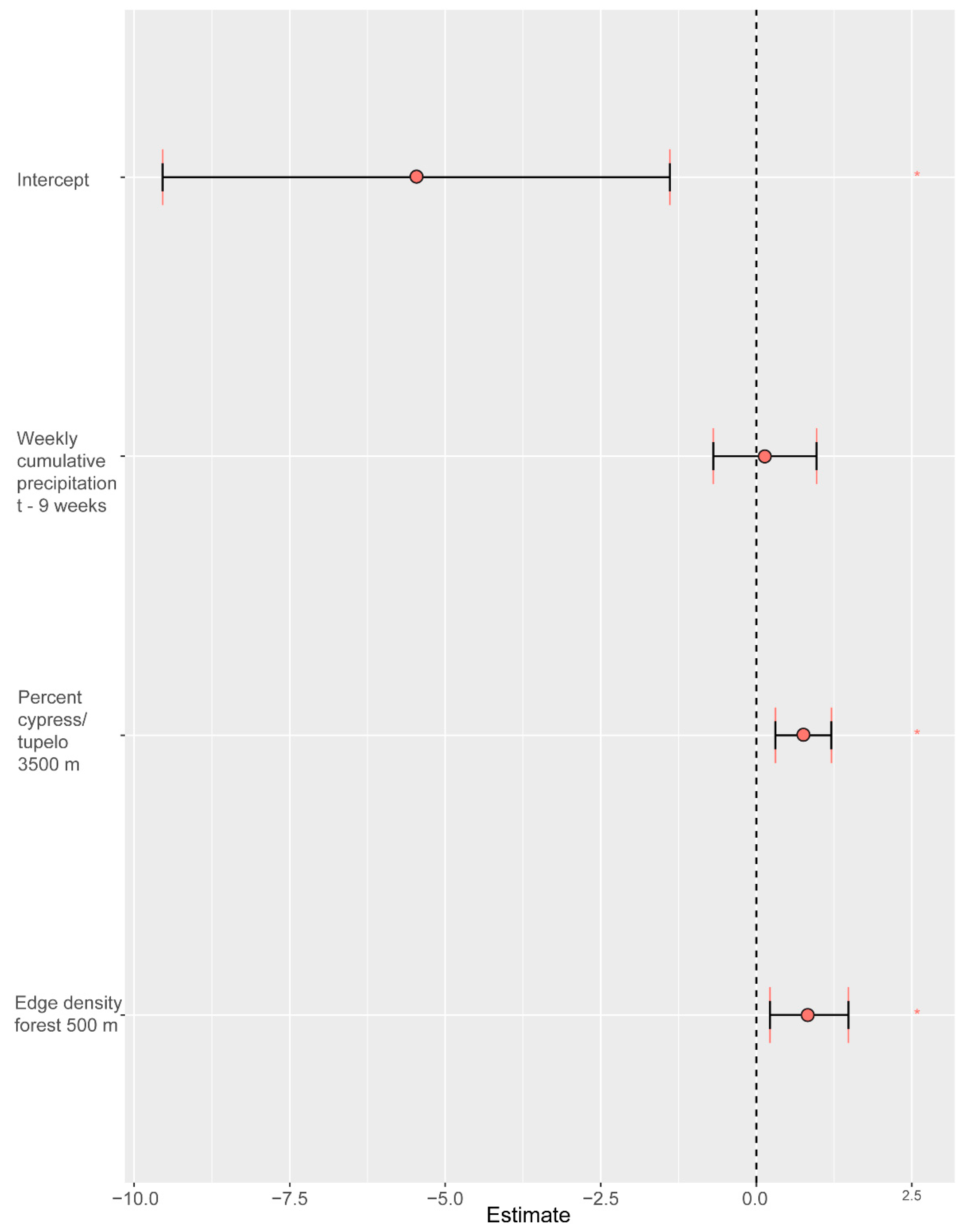
| Model Rank 1 (Best) | |||
|---|---|---|---|
| mean | 0.025 quant | 0.975 quant | |
| Intercept | −5.4651 | −9.5433 | −1.3903 |
| Weekly cumulative precip t − 9 | 0.1386 | −0.6905 | 0.967 |
| 3500 m percent cypress–tupelo wetland | 0.7552 | 0.3056 | 1.2045 |
| 500 m edge density forest | 0.8507 | 0.2203 | 1.4806 |
| Model Rank 2 | |||
| mean | 0.025 quant | 0.975 quant | |
| Intercept | −5.406 | −8.958 | −1.856 |
| Weekly cumulative precip t − 9 | 0.168 | −0.662 | 0.999 |
| 500 m edge density forest | 0.782 | 0.136 | 1.426 |
| 3500 percent cypress–tupelo wetland | 0.765 | 0.299 | 1.231 |
| Weekly cumulative precip t − 1 | 0.309 | −0.246 | 0.864 |
| Model Rank 3 | |||
| Value | mean | 0.025 quant | 0.975 quant |
| Intercept | −5.199 | −8.257 | −2.144 |
| Weekly cumulative precip t − 9 | 0.082 | −0.68 | 0.843 |
| 5000 m percent forest | 0.456 | −0.141 | 1.051 |
| 3500 m percent cypress–tupelo wetland | 0.531 | 0.005 | 1.057 |
| Model Rank 1 (Best) | |||
|---|---|---|---|
| Value | mean | 0.025 quant | 0.975 quant |
| Intercept | −3.687 | −6.468 | −0.909 |
| Model Rank 2 | |||
| Value | mean | 0.025 quant | 0.975 quant |
| Intercept | −3.721 | −6.542 | −0.902 |
| Weekly cumulative precip t − 1 | 0.001 | −0.591 | 0.591 |
| Weekly cumulative precip t − 3 | −0.111 | −0.67 | 0.447 |
| Model Rank 3 | |||
| mean | 0.025 quant | 0.975 quant | |
| Intercept | −3.71 | −6.42 | −1.002 |
| 2000 m edge density wetland | −0.128 | −0.476 | 0.219 |
| Weekly cumulative precip t − 1 | −0.005 | −0.595 | 0.585 |
| Weekly cumulative precip t − 3 | −0.117 | −0.676 | 0.441 |
| Model Rank 4 | |||
| mean | 0.025 quant | 0.975 quant | |
| Intercept | −3.717 | −6.469 | −0.968 |
| 3500 m edge density wetland | −0.1 | −0.438 | 0.237 |
| Weekly cumulative precip t − 1 | −0.002 | −0.593 | 0.587 |
| Weekly cumulative precip t − 3 | −0.115 | −0.673 | 0.444 |
| Model Rank 5 | |||
| mean | 0.025 quant | 0.975 quant | |
| Intercept | −3.717 | −6.469 | −0.968 |
| 5000 m edge density wetland | −0.1 | −0.438 | 0.237 |
| Weekly cumulative precip t − 1 | −0.002 | −0.593 | 0.587 |
| Weekly cumulative precip t − 3 | −0.115 | −0.673 | 0.444 |
| Model Rank 6 | |||
| mean | 0.025 quant | 0.975 quant | |
| Intercept | −3.717 | −6.574 | −0.862 |
| Weekly cumulative precip t − 1 | 0.011 | −0.587 | 0.608 |
| Weekly cumulative precip t − 3 | −0.101 | −0.663 | 0.46 |
| Weekly cumulative precip t − 7 | 0.088 | −0.376 | 0.552 |
Publisher’s Note: MDPI stays neutral with regard to jurisdictional claims in published maps and institutional affiliations. |
© 2022 by the authors. Licensee MDPI, Basel, Switzerland. This article is an open access article distributed under the terms and conditions of the Creative Commons Attribution (CC BY) license (https://creativecommons.org/licenses/by/4.0/).
Share and Cite
Campbell, L.P.; Guralnick, R.P.; Giordano, B.V.; Sallam, M.F.; Bauer, A.M.; Tavares, Y.; Allen, J.M.; Efstathion, C.; Bartlett, S.; Wishard, R.; et al. Spatiotemporal Modeling of Zoonotic Arbovirus Transmission in Northeastern Florida Using Sentinel Chicken Surveillance and Earth Observation Data. Remote Sens. 2022, 14, 3388. https://doi.org/10.3390/rs14143388
Campbell LP, Guralnick RP, Giordano BV, Sallam MF, Bauer AM, Tavares Y, Allen JM, Efstathion C, Bartlett S, Wishard R, et al. Spatiotemporal Modeling of Zoonotic Arbovirus Transmission in Northeastern Florida Using Sentinel Chicken Surveillance and Earth Observation Data. Remote Sensing. 2022; 14(14):3388. https://doi.org/10.3390/rs14143388
Chicago/Turabian StyleCampbell, Lindsay P., Robert P. Guralnick, Bryan V. Giordano, Mohamed F. Sallam, Amely M. Bauer, Yasmin Tavares, Julie M. Allen, Caroline Efstathion, Suzanne Bartlett, Randy Wishard, and et al. 2022. "Spatiotemporal Modeling of Zoonotic Arbovirus Transmission in Northeastern Florida Using Sentinel Chicken Surveillance and Earth Observation Data" Remote Sensing 14, no. 14: 3388. https://doi.org/10.3390/rs14143388
APA StyleCampbell, L. P., Guralnick, R. P., Giordano, B. V., Sallam, M. F., Bauer, A. M., Tavares, Y., Allen, J. M., Efstathion, C., Bartlett, S., Wishard, R., Xue, R.-D., Allen, B., Tressler, M., Qualls, W., & Burkett-Cadena, N. D. (2022). Spatiotemporal Modeling of Zoonotic Arbovirus Transmission in Northeastern Florida Using Sentinel Chicken Surveillance and Earth Observation Data. Remote Sensing, 14(14), 3388. https://doi.org/10.3390/rs14143388