Cloud Removal with SAR-Optical Data Fusion and Graph-Based Feature Aggregation Network

Abstract

In observations of Earth, the existence of clouds affects the quality and usability of optical remote sensing images in practical applications. Many cloud removal methods have been proposed to solve this issue. Among these methods, synthetic aperture radar (SAR)-based methods have more potential than others because SAR imaging is hardly affected by clouds, and can reflect ground information differences and changes. While SAR images used as auxiliary information for cloud removal may be blurred and noisy, the similar non-local information of spectral and electromagnetic features cannot be effectively utilized by traditional cloud removal methods. To overcome these weaknesses, we propose a novel cloud removal method using SAR-optical data fusion and a graph-based feature aggregation network (G-FAN). First, cloudy optical images and contemporary SAR images are concatenated and transformed into hyper-feature maps by pre-convolution. Second, the hyper-feature maps are inputted into the G-FAN to reconstruct the missing data of the cloud-covered area by aggregating the electromagnetic backscattering information of the SAR image, and the spectral information of neighborhood and non-neighborhood pixels in the optical image. Finally, post-convolution and a long skip connection are adopted to reconstruct the final predicted cloud-free images. Both the qualitative and quantitative experimental results from the simulated data and real data experiments show that our proposed method outperforms traditional deep learning methods for cloud removal.

1. Introduction

With the development of information technology and the increasing number of optical imaging satellites, a great deal of optical remote sensing data with abundant spatial and spectral information has been provided. Optical satellite remote sensing data has been widely employed to investigate Earth’s surface in applications such as urban construction, disaster assessment, environmental protection, and cropland monitoring [1,2,3,4,5]. As important remote sensing data in observations of Earth, optical imagery has the advantages of being suitable for human vision, a high spatial resolution, and rich spectral information. However, optical remote sensing images are often contaminated by clouds and accompanying shadows, which restrict subsequent data analysis and employment [6,7]. According to the statistics of Landsat ETM+ data produced by [8], 35% of Earth’s surface is covered by clouds throughout the year, and this percentage is even larger in the ocean. The large-scale and frequent existence of clouds leads to application value reductions of many optical remote sensing images, which obstructs the scientific research and engineering applications of remote sensing data [9]. Therefore, it is necessary to carry out cloud removal in optical remote sensing images so as to effectively remove the influence of clouds, restore precise spatial and spectral information of the surface, and improve the integrity and availability of the remote sensing data. Generally, the operation of cloud removal can be divided into two steps: cloud detection [10,11,12] and missing data reconstruction. Cloud detection is the identification and masking of cloud-contaminated pixels, while missing data reconstruction fills missing data gaps produced by cloud detection. In this paper, our work mainly focuses on the second step of cloud removal.

Among the various forms of clouds, thick clouds often completely obscure the optical information reflected by the surface, and have become the focus of cloud removal. Among the many remote sensing approaches, the electromagnetic wave used in synthetic aperture radar (SAR) imaging is hardly affected by clouds, and has the ability to provide all-weather observations of Earth. With the development of SAR imaging technology, SAR images have also been widely applied in the fields of information extraction, interpretation, and quantitative analysis, which has been recognized by many scholars [13,14,15]. Therefore, combined with the characteristics and advantages of SAR imaging, this paper proposes a novel method for cloud removal with SAR-optical data fusion and a graph-based feature aggregation network (G-FAN).

In the past decades, many cloud and cloud shadow removal approaches have been proposed to reconstruct missing and degraded data in remote sensing images. According to the relevant literature, these approaches can be divided into three major categories: (1) spatial information-based methods; (2) temporal information-based methods; (3) multi-source auxiliary information-based methods. Moreover, according to mechanism and model of the data reconstruction, these methods can be divided into traditional methods and deep learning methods. We will introduce the related works using the abovementioned classification criteria.

(1)

Spatial information-based methods

Spatial information-based methods assume that the remaining cloud-free regions have similar texture features and spectral features as cloud-contaminated regions. Spatial information-based methods typically deal with cloud contamination in a single image without additional temporal or auxiliary information. Traditional mathematical models based on statistics and deep learning methods are used in the processing of cloud removal. Maalouf et al. [16] proposed the use of the multi-scale geometry feature of the images’ structures to reconstruct the missing data or the cloud-contaminated region. Zheng et al. [17] proposed U-Net and the generative adversarial network (GAN) to extract the clouds, remove thin clouds, and recover thick cloud-contaminated regions, but this is not fit for images with a large cloud cover area. Meng et al. [18] presented the sparse dictionary learning method for recovering missing information caused by clouds. Generally, spatial information-based methods are efficient and perform well in reconstructing small areas of missing data or regions with a regular texture. However, the reconstruction precision cannot be guaranteed, especially for high-frequency texture areas or the boundary between the different land surfaces.

(2)

Temporal information-based methods

Temporal information-based methods require additional clear images as auxiliary data to reconstruct the cloud-covered area, and are reliant on the fact that time series data are strictly chronological and display regular fluctuations. In order to obtain a good visual scene, many traditional image processing methods, such as brightness and chromaticity adjustment, linear spectral unmixing, color matching, and multi-scale wavelet-based fusion, have been adopted to optimize the results of temporal information-based methods. Many classical models and methods, such as multi-temporal dictionary learning [7], sparse representation [19], non-negative matrix factorization [20], and autoregression [21], have been introduced into cloud removal in remote sensing image sequences.

In recent years, many deep learning models based on temporal information have also been adopted for the development of cloud removal. For example, a spatial–temporal–spectral deep convolutional neural network [22], fully convolutional network with a channel attention mechanism [23], and generative adversarial networks [24] have been proposed and used to remove clouds and reconstruct the missing data. In general, combined with deep learning, temporal information-based methods achieve good reconstruction results for cloud-covered regions without a rapid or significant surface change or phenological change. However, cloud-free time series images or references of high quality are difficult to acquire, which is the main bottleneck restricting the wide application of temporal information-based methods in actual engineering.

(3)

Multi-source auxiliary information-based methods

In addition to the abovementioned cloud removal methods that use homogeneous data as a reference, a few researchers have attempted to explore multi-source auxiliary data for cloud removal in remote sensing images. Multi-source auxiliary information-based methods utilize optical images from a different sensor or SAR images to make up for the lack of available auxiliary data, and they enhance the ability to reconstruct areas with land cover changes. Shen et al. [25] developed a cloud removal procedure based on multi-source data fusion to overcome the poor performance of temporal information-based methods in cases with significant land cover changes. Angel et al. [26] reconstructed cloud-contaminated pixels, based on multi-temporal hyperspectral imagery, and a geostatistical model, according to the spatio–temporal correlation between them.

A deep residual neural network architecture, called DSen2-CR, was designed to remove clouds from multi-spectral Sentinel-2 imagery in [27], and SAR-optical data fusion was used to exploit the synergistic properties of the two imaging systems to guide the image reconstruction. The proposed method even allowed the removal of thick clouds by reconstructing an optical representation of the underlying land surface structure. Grohnfeldt [28], Bermudez [29], Gao [30], and He [31] et al. presented various improved generative adversarial networks for cloud removal that were specifically designed to generate cloud-free multi-spectral optical data from a cloud-corrupted multi-spectral input and an auxiliary SAR image. Eckardt et al. [32] presented a method for the reconstruction of pixels contaminated by optical thick clouds in multi-spectral Landsat images using multi-frequency SAR data from TerraSAR-X (X-Band), ERS (C-Band), and ALOS Palsar (L-Band); furthermore, their results indicate the potential of multi-frequency SAR images for use in cloud removal in multi-spectral images. Generally, SAR-based methods used to reconstruct missing data are more common, and have more potential than other multi-source auxiliary information-based methods because the microwave signal is more capable of penetrating clouds, and it there is a greater possibility for land surface change, fine texture, and tiny ground object reconstruction.

Considering the merits and demerits of traditional and deep learning methods, and inspired by the performance of the SAR-based method, in this paper, we propose a novel graph-based feature aggregation network to remove thick clouds and cloud shadows from multi-spectral Sentinel-2 images by exploiting SAR images from Sentinel-1 and optical images from Sentinel-2 satellites. The main contributions of the proposed method are summarized as follows:

■

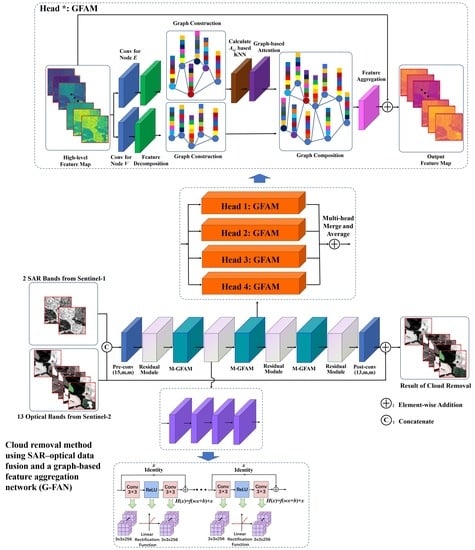
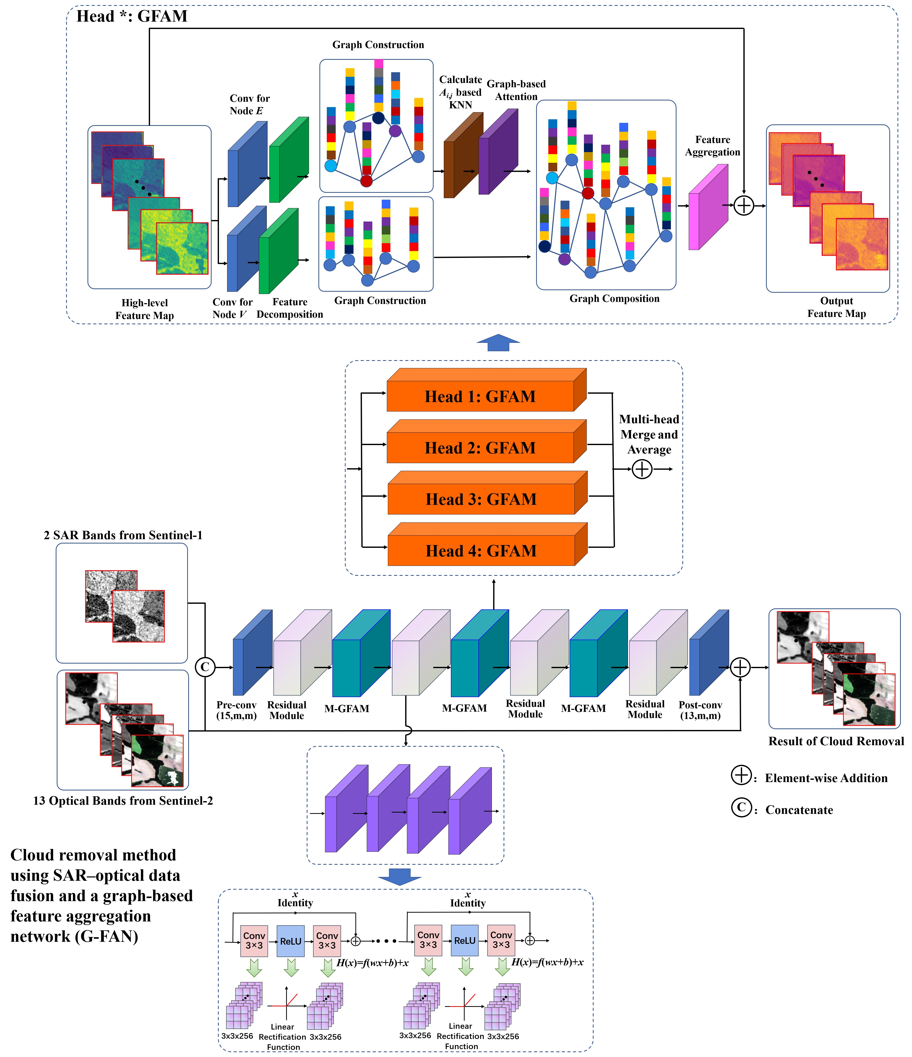
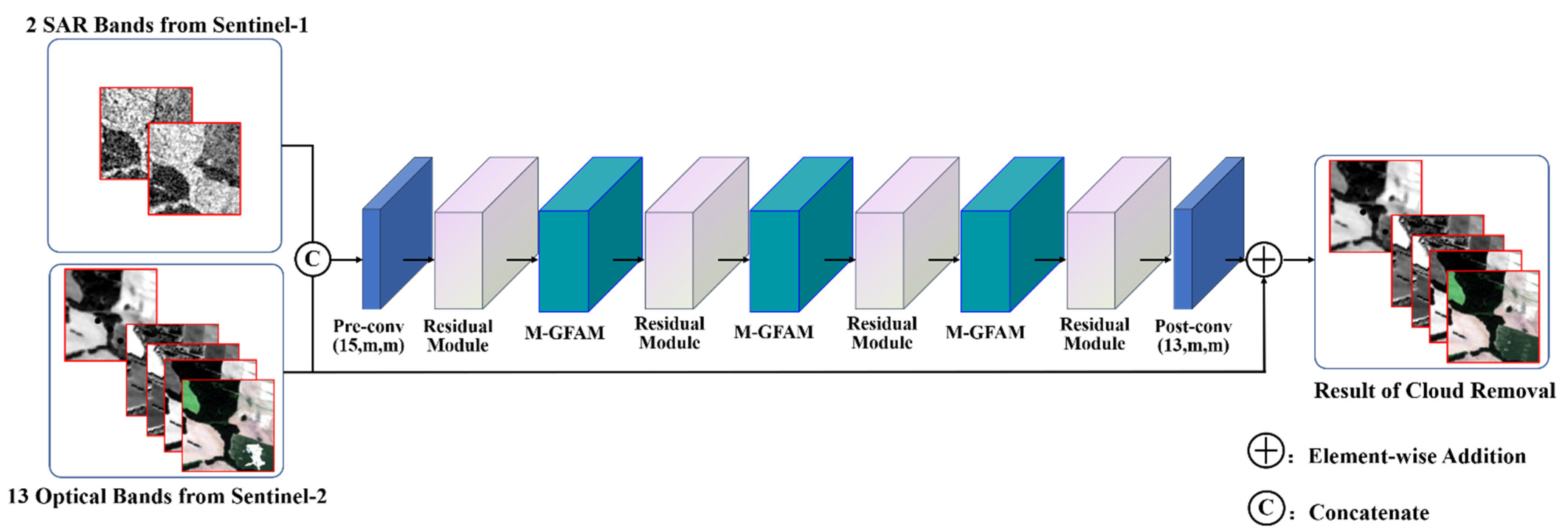
Based on deep learning theory and data-driven principles, we propose a novel deep neural network called G-FAN to remove thick clouds and cloud shadows in Sentinel-2 satellite optical images with contemporary SAR images from the Sentinel-1 satellite. The proposed deep neural network, combined with the advantages of the residual network (ResNet) and graph attention network (GAT), utilizes SAR imaging without the influence of clouds in order to reconstruct multi-band reflectance in optical remote sensing images by learning and extracting the non-linear correlation between the electromagnetic backscattering information in the SAR images, the spectral information of the neighborhood pixels, and the non-neighborhood pixels in the optical images.

■

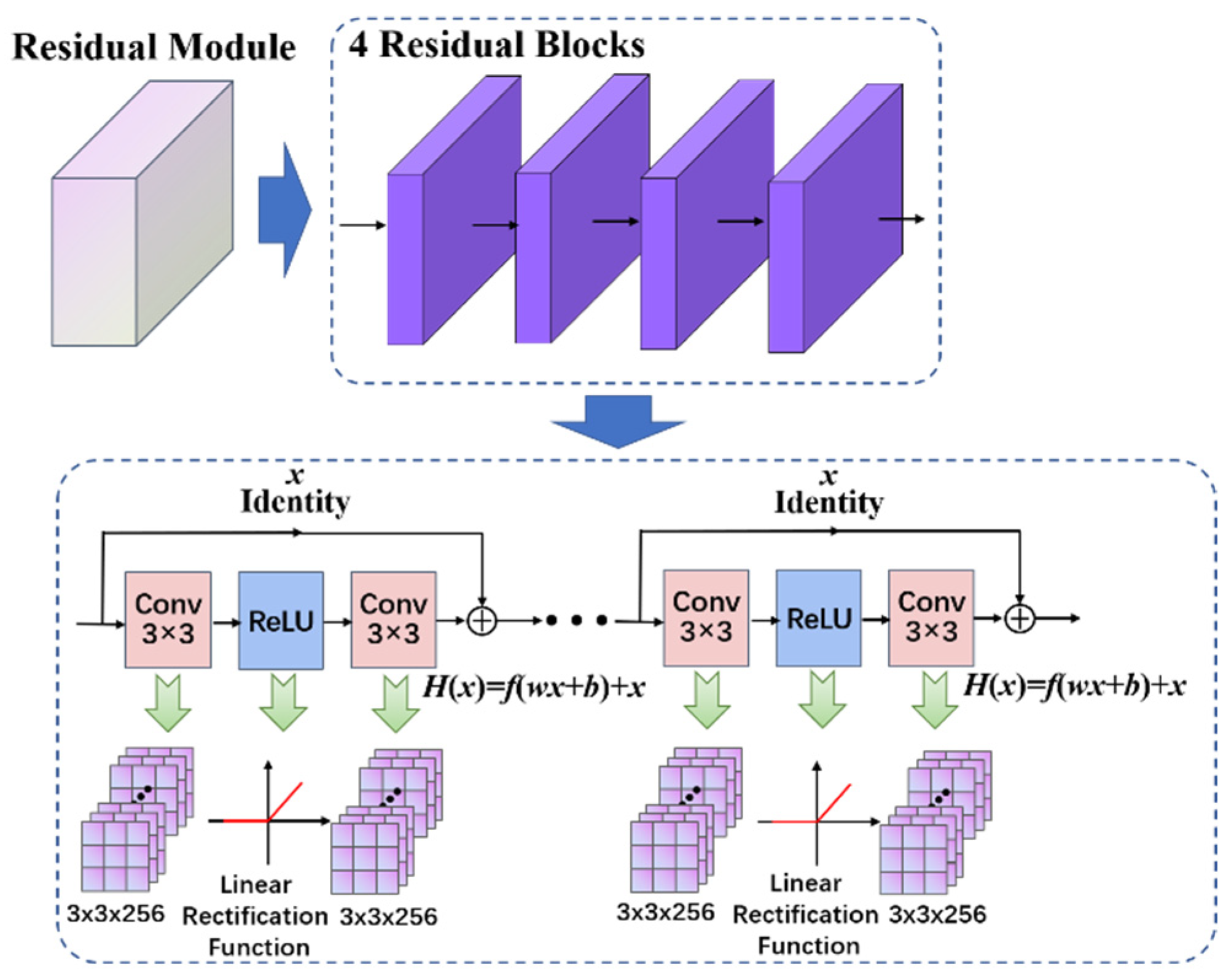
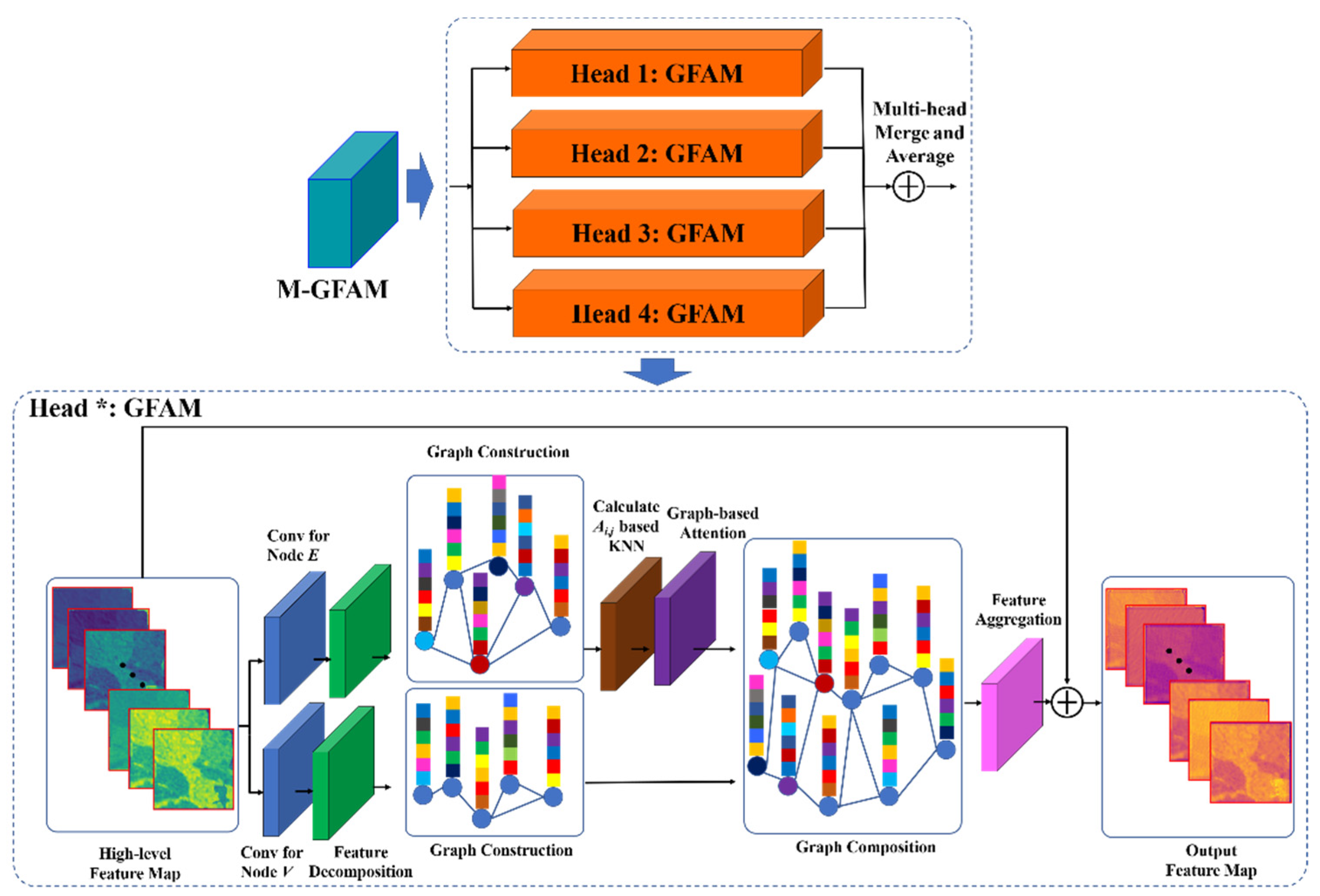
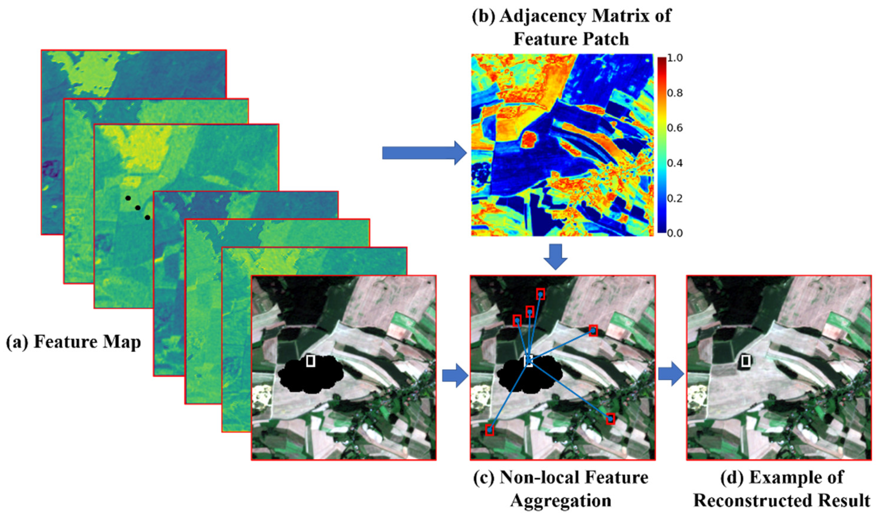
Since SAR images used as auxiliary data for cloud removal may be blurred and noisy, and the convolution of the traditional deep learning model for cloud removal mainly uses neighborhood information, spectral information and electromagnetic backscattering information (i.e., non-neighborhood information) cannot be effectively used. A feature information aggregation method based on the graph attention mechanism is proposed for cloud removal and restoration of remote sensing images. A proposed network architecture, in which the multi-head graph-based feature aggregation modules (M-GFAM) and residual modules are constructed alternately, achieves the simultaneous processing of cloud removal, image deblurring, and image denoising.

■

A loss function based on the smooth L1 loss function and the Multi-Scale Structural Similarity Index (MS-SSIM) is proposed and used in our model. The smooth L1 loss function is used as a basic error function to reduce the gap between the predicted cloud-free image and the ground truth image. When the error between the predicted value and the true value becomes smaller, our model can obtain a smooth and steady gradient descent. Equipped with MS-SSIM, our loss function is more suitable for the human visual system than others, and can maintain a stable performance in remote sensing images with different resolutions.

The structure of this paper is as follows: Section 2 introduces the proposed G-FAN method, which mainly includes our framework for cloud removal tasks, residual module construction, the GAT, the application of the graph-based feature aggregation mechanism, and loss function. Section 3 provides some simulated data experiments, real data experiments, and ablation experiments to show the superiority of the proposed approach. Section 4 presents a further discussion on overfitting, computation complexity, and different cloud detection methods of the proposed network. Finally, Section 5 summarizes the conclusion. An abbreviations list and Appendix A containing figures are also provided.

2. Methods

2.1. Overview of the Proposed Framework

The whole architecture of our proposed G-FAN is displayed in Figure 1, which is made up of two major components: four residual modules and three M-GFAM. Inspired by DSen2-CR based on ResNet for cloud removal in [27], we added M-GFAM in ResNet with residual modules at regular intervals in order to aggregate the similar non-local features in feature maps. The residual module was used to fuse the spectral–electromagnetic–spatial features by a multi-layer 3 $\times$ 3 convolution and a skip connection; the graph-based feature aggregation module (GFAM) in the M-GFAM aim to extract and aggregate similar non-local features in hyper-cubic images, which denotes spectral–electromagnetic–spatial information in Sentinel-2 multi-band imagery and Sentinel-1 SAR imagery.

The residual modules in our G-FAN with skip connection produce a series of hierarchy features, which are extracted by multilayer convolutions and activation functions, as the conclusion in [27], this architecture of deep learning can achieve the basic function of cloud removal, while SAR images used as auxiliary information in [27] may be blurred and noisy, the similar non-local information of spectral and electromagnetic features cannot be effectively utilized in the model of [27]. To solve this problem, we proposed to add M-GFAM in ResNet. The GFAM is the core of our proposed G-FAN, which was implemented based on a graph attention network [33]. The GFAM can aggregate similar non-local features in feature space to reconstruct the missing data area contaminated by clouds, so that our approach achieves simultaneous processing of cloud removal and image quality improvement. More details on G-FAN will be provided in the following subsection.

2.2. Residual Module Construction

ResNet effectively utilizes features of the initial layers and alleviates the gradient vanishing problem by adding a skip connection, which has been successfully applied to many computer vision tasks, such as image classification, segmentation, object recognition, and image restoration. As shown in Figure 1, our proposed model is built on residual modules and M-GFAM. The residual modules are the main elements and function modules of ResNet. In our model, each residual module contains four residual blocks (shown in Figure 2). Each residual block extracts the feature information of neighborhood points by two layers of a 3 $\times$ 3 convolution, a ReLU function, and a skip connection, and the feature information of the input layer is obtained.

According to the theory of ResNet, skip connection is the core of the residual module. When the neural network contains a skip connection, the desired underlying mapping $H\left(x\right)$ can be defined as:

$$H\left(x\right)=f(\mathit{wx}+b)+x$$

(1)

where the $x$ is input, $\mathit{w}$ is the weight of the layer, $b$ is the offset, and $f\left(\cdot \right)$ is the activation function.

In general, the feature dimension of the input may be the same as those of the output in the skip connection. Multiple residual blocks in our proposed model generate a series of hierarchy features. The features of the last layer are used for image reconstruction in the cloud-covered region. However, the features of shallow layers also contain a lot of information that can be utilized. Shallow layers produce weak features, which are extracted by fewer residual blocks. These weak features obtain more detailed information for original optical and SAR images. At the same time, deep layers produce strong features, which are aggregated by more residual blocks. These strong features characterize the abstract correlation between feature vectors in high-dimension feature space.

2.3. Graph Attention Network

Graphs represent the fundamental data structure, and appear in different application fields. They allow one to gather correlations among data, and are a natural way of representing real-world information. Traditional machine learning and deep learning models are typically constrained to a regular data structure, such as a grid or sequences (defined in Euclidean space), and do not adapt to the complexity of graphs (non-Euclidean space) [34]. In our proposed approach for cloud removal and remote sensing image restoration, the missing data of cloud-contaminated regions have a neighborhood correlation in the spatial–spectral–electromagnetic feature space as a Euclidean space, which the traditional deep convolutional neural networks can directly deal with. However, a non-neighborhood correlation in spatial–spectral–electromagnetic feature space as non-Euclidean space is more easily extracted and dealt with by a graph convolutional network (GCN).

The graph $\mathcal{G}=\left(\mathcal{V},\mathcal{E}\right)$ consists of a set of nodes $\mathcal{V}=\left\{v_1{,v}_2,\cdots v_N\right\}$ and a set of edges $\mathcal{E}=\left\{e_{11}{,e}_{12},\cdots e_{\mathit{NN}}\right\}$, where $N$ is the number of nodes in the graph, and node $v_i\in {ℝ}^d$ is a feature vector with the dimension of $d$. Accordingly, the feature vectors in the feature map and their similarities can be directly seen as nodes and edges in a graph, respectively. The adjacency matrix, $A$, is usually used to define the graph structure in order to represent the similarities between feature vectors [35,36,37], which can be computed by:

$$A_{i,j}=\exp \left(-\frac{\Vert v_i{-v}_j\Vert {}^2}{{\mathsf{\sigma }}^2}\right)$$

(2)

where $v_i$ and $v_j$ denote two feature vectors corresponding to two different feature patches, and $\mathsf{\sigma }$ is the width of the radial basis function. Using Equation (3), the Laplacian matrix $L$ can be obtained by $L=D - W$, where $D$ denotes the diagonal matrix given by $D_{i,i}={\displaystyle \sum }_j{A}_{i,j}$. According to [38], the propagation rule from the $l$-th layer to the ($l+1$)-th layer in GCN can be denoted as follows:

$$H_A^{(l+1)}{=f( \tilde{D} }^{-\frac{1}{2}}{ \tilde{A} \tilde{D} }^{-\frac{1}{2}}{H}_A^{\left(l\right)}{W}_A^{\left(l\right)}{+b}_A^{\left(l\right)})$$

(3)

where $H_A^{\left(l\right)}$ denotes the hidden representations in the $l$-th layer with the variables $W_A^{\left(l\right)}$ and $b_A^{\left(l\right)}$. Moreover, $\tilde{A}$ denotes the normalized adjacency matrix, $A_{i,j}$ in Equation (2).

Using Equation (3) to replace the traditional layer-wise propagation rule in CNN, the GCN can be also used for remote sensing image reconstruction.

The GAT is derived from the GCN method and the attention mechanism. The aim of using the attention mechanism is to find those that are more important in the current task and to distribute them with higher weights, called attention scores. In this way, each node can aggregate the feature information selectively from all of its connected neighbors. After linear transformation to a new feature space by the projection matrix $\tilde{W} \in {ℝ}^{C\times d}$, the correlation, $e_{i,j}$, between node $v_i$ and its neighborhood node, $v_j$, can be revealed by a simple but effective single-layer neural network. The correlation, $e_{i,j}$, corresponding attention coefficients, ${\alpha }_{i,j}$, and the graph convolution output of each node, $v_i^l$, has the following expression [34,37,38]:

$$\left\{\begin{array}{l}{e}_{i,j}=LeakyReLU\left({\omega }^T\left[{\tilde{W}}^T{v}_i\left|\right|{\tilde{W}}^T{v}_j\right]\right) \\ {\mathit{\alpha }}_{i,j}=\frac{\exp \left(\mathit{LeakyReLU}\left({\omega }^T\left[{ \tilde{W} }^T{v}_i{\left|\right| \tilde{W} }^T{v}_j\right]\right)\right)}{{{\displaystyle \sum }}_{k\in N_i}\exp \left(\mathit{LeakyReLU}\left({\omega }^T\left[{ \tilde{W} }^T{v}_i{\left|\right| \tilde{W} }^T{v}_k\right]\right)\right)}\\ v_i^l=f\left({\displaystyle {\displaystyle \sum }_{j\in N_i}}{\alpha }_{i,j}{ \tilde{W} }^T{v}_j^{l-1}\right) \end{array}\right.$$

(4)

where $\omega \in {ℝ}^{2d}$ is the parameter vector of the network, $\left|\right|$ denotes the concatenation operation, LeakyReLU(·) is a non-linear function, $f\left(\cdot \right)$ is the activate function, and $\tilde{W}$ is the filtering matrix for the dimension reduction and feature extraction of the initial feature map.

2.4. Application of the Graph-Based Feature Aggregation Mechanism

In this study, we used graph construction and the multi-head attention mechanism to design novel and versatile feature aggregation modules, called M-GFAMs, which contain four GFAMs (shown in Figure 3). The model equipped with GFAMs performs well in extracting non-local feature information and learning to generate new features, instead of merely extracting features from neighbors of the input via the traditional convolution operation in ResNet. Applying the strategy of multi-information fusion on SAR and optical images, our model, combined with GFAM, can make up for the limitations of SAR with insufficient band information, to a certain extent, and enhance the ability of information extraction and the precision of cloud removal.

The traditional residual module and attention mechanism have proven to be useful for image inpainting, image denoising, and image restoration [39,40,41,42]. We favor feature aggregation based on the graph attention model over residual connections here, since the former utilizes features from previous feature layers, as well as different non-local features from itself (a visual example is shown in Figure 4). The proposed GFAM focuses on the most relevant feature vector in order to make effective decisions by specifying different weights for different nodes of the graph, and has a single-layer attention mechanism; therefore, it has fewer learning network parameters and a smaller computational load with each training iteration. The attention layer in the GFAM is situated after the convolution layers of the residual module, which, firstly, allows the use of learned attention weights to readjust the feature map so that the following convolution layers of the residual module can pay more attention to the significant nodes, and, secondly, this structure prevents the negative influence of noisy information from the context nodes for the attention coefficients. This approach consists of three phases: graph-based feature extraction and modeling, dynamic graph connection optimization, and graph-based feature aggregation with multi-head attention.

2.4.1. Graph-Based Feature Extraction and Modeling

In our GFAM, we first constructed an undirected and connected graph, $\mathcal{G}=\left(\mathcal{V},\mathcal{E}\right)$, on regular grid data by discretizing the organized features in the feature maps outputted by the previous residual module, where $\mathcal{V}$ is the set of nodes. Each node in $\mathcal{V}$ denotes a feature vector of a small patch. The total of $\mathcal{V}$ is $N$, and $\mathcal{E}\in \mathcal{V}\times \mathcal{V}$ is the set of edges. The element $e_{i,j}$ of the $\mathcal{E}$ set denotes the edge from node $v_i$ and node $v_j$ in the set of $\mathcal{V}$, which is measured by a specific feature space distance function. Assuming $N$ overlaps feature patches $v_i$, with the patch size being ${C\times W}_p{\times H}_p$, where $C$, $W_p$, and $H_p$ are, respectively, the channel, width, and height of the patch, neatly arranged in the input feature map, $F_{\mathit{in}}\in {ℝ}^{C\times W\times H}$. Two 1 $\times$ 1 convolutional layers ($f_{\mathit{edge}}$ and $f_{\mathit{node}}$) are introduced to transform $F_{\mathit{in}}$ into two independent representations, and then the unfold operation is utilized to extract the transformed feature patches as two groups: $G^{\prime }={\left\{p_i^{\prime }\right\}}_{i=1}^N$ and $G^{″}={\left\{p_i^{″}\right\}}_{i=1}^N$, in which $G^{\prime }$ is used to build graph connections, $\mathcal{E}$, and $G^{″}$ is assigned as the graph nodes, $\mathcal{V}$. Each feature patch in $G^{\prime }$ and $G^{″}$ can be denoted as follows:

$$\left\{\begin{array}{c}{p}_i^{\prime }=f_{\mathit{edge}}\left(v_i\right) \\ p_i^{″}=f_{\mathit{node}}\left(v_i\right)\end{array} \right.$$

(5)

2.4.2. Dynamic Graph Connection Optimization

According to the mechanism of the GAT, the graph nodes are directly assigned by feature patches in $G^{″}$: $\mathcal{V}=G^{″}$. In establishing graph connections, the dynamic number of neighbors for each node is selected, based on the nearest principle, in order to selectively preserve the important nodes and reduce the adverse influence of redundant, unimportant nodes. For this purpose, a dynamic KNN method was introduced to generate an adaptive threshold for each node to select neighbors whose similarities are above the threshold. Specifically, given the set of feature patches, $G^{\prime }$, each feature patch, $p_i^{\prime }$ in $G^{\prime }$ is flattened into a feature vector. The pair-wise similarity, $m_{\mathit{ij}}$, of $p_i^{\prime }$ and $p_j^{\prime }$ can be calculated by the dot product, producing a similarity matrix, $\mathit{M}=\left[{\mathit{m}}_{11}{,\mathit{m}}_{12},\cdots {\mathit{m}}_{\mathit{NN}}\right]$ and $\mathit{M}\in {ℝ}^{N\times N}$. Furthermore, ${\mathit{M}}_i$, the $i$-th row of $\mathit{M}$, represents similarities between the $i$-th node and the other nodes. The average of ${\mathit{M}}_i$ is the average importance of different nodes to the $i$-th node. In order to choose an appropriate threshold to improve the adaptability of the proposed model, a node-specific affine transformation was adopted to calculate $T_i$:

$$T_i=\frac{{\mathit{\psi }}_1\left(p_i^{\prime }\right)}{N}{\displaystyle \sum }_{k=1}^N{\mathit{M}}_{i,k}+{\mathit{\psi }}_2\left(p_i^{\prime }\right)=\frac{\mathit{\gamma }}{N}{\displaystyle \sum }_{k=1}^N{\mathit{M}}_{i,k}+\mathit{\beta }$$

(6)

where ${\mathit{\psi }}_1$ and ${\mathit{\psi }}_2$ are two independent convolutional layers, with the kernel size being ${C\times 1\times W}_p{\times H}_p$ to embed each node to specific affine transformation parameters ($\mathit{\beta }$, $\mathit{\gamma }$). Then, a ReLU function was utilized to truncate feature paths less than $T_i$. The new adjacency matrix A can be denoted as:

$$A_{i,:}=\mathrm{ReLU}\left({\mathit{M}}_{i,:}-T_i\right)$$

(7)

where $A\in {ℝ}^{N\times N}$, and $A_{i,j}$ is assigned the similarity weight if $p_j^{\prime }$ connects to $p_i^{\prime }$ and the similarity weight is greater than $T_i$; otherwise, it is equal to zero. Then, following the attention mechanism shown in Equation (4), we normalized the similarity of all the connected nodes (non-zero values in $A_{i,j}$) using the softmax function to compute the attention weights:

$${\mathit{\alpha }}_{i,j}=\frac{\exp \left(A_{i,j}\right)}{{{\displaystyle \sum }}_{k\in N_i}\exp \left(A_{i,k}\right)}, j\in N_i$$

(8)

2.4.3. Graph-Based Feature Aggregation with Multi-Head Attention

According to the graph-based attention mechanism and network introduced in Section 2.3, we adopted a feature aggregation process for the weighted sum of all the connected neighbors in the adjacency matrix, $A$; the new feature path ${\hat{p}}_i$ optimized by graph-based feature aggregation can be formulated by:

$${\hat{p}}_i={\displaystyle \sum }_{j\in N_i}{\alpha }_{i,j}\cdot p_j^{″}={\displaystyle \sum }_{j\in N_i}{\alpha }_{i,j}\cdot f_{\mathit{node}}\left(v_j\right)$$

(9)

Then, we extracted all the feature patches from the graph and utilized the fold operation to combine this array of updated local patches into a feature map, which can be viewed as the inverse of the unfold operation. Since there existed overlaps between feature patches, we used the average operation to deal with the overlapping areas. This strategy can also suppress the blocking effect in the final output. Inspired by the skip connection in ResNet, we constructed a global residual connection in each GFAM to further enhance the output; thus, the output of the GFAM is denoted as:

$$F_{\mathit{out}}=F_{\mathit{in}}+\mathit{Fold}\left({\left\{{\hat{p}}_i\right\}}_{i=1}^N\right)$$

(10)

To further stabilize the attention mechanism of the GFAM, inspired by the multi-head attention mechanism in [33], we employed the $K$-independent attention operations of Equation (10) on the neighborhood nodes. Then, the $K$ results were averaged to obtain the final neighborhood node, once again projected by a $1 \times 1$ convolutional layer ($f_{\mathit{merge}}$). The final result, $F_{\mathit{out}}^{\mathit{MH}}$, optimized by the multi-head attention mechanism is expressed as:

$${F }_{\mathit{out}}^{\mathit{MH}}=f_{\mathit{merge}}\left(\frac{1}{K }{\displaystyle \sum }_{k=1}^K{F}_{\mathit{out}}^k\right)$$

(11)

where $F_{\mathit{out}}^k$ is the output of the $k$-th head. $K$ is 4 in our proposed network.

2.5. Loss Function of G-FAN

We refer the loss function of the proposed G-FAN as $L_{\mathrm{G}-\mathrm{FAN}}$, and it was employed in the optimization of parameters in the proposed network. To reduce the gap between the generated clear image and the ground truth image, and to obtain a good visual perception, the total loss function of $L_{G-\mathrm{FAN}}$ consists of a smooth $L_1$ loss function and $L_{\mathrm{MS}-\mathrm{SSIM}}$ loss function. $L_{G-\mathrm{FAN}}$ is formulated as:

$$L_{G-\mathrm{FAN}}\left(\mathit{P},T\right)=L_{{\mathrm{Smooth} L}_1}\left(\mathit{P},T\right)+\lambda L_{\mathrm{MS}-\mathrm{SSIM}}\left(\mathit{P},T\right)$$

(12)

where $\mathit{P}$ is the predicted image, and $T$ is the cloud-free target image; $L_{{\mathrm{Smooth} L}_1}$ is the smooth $L_1$ loss function; $L_{\mathrm{MS}-\mathrm{SSIM}}$ is a loss function based on the MS-SSIM; and $\lambda$ is the weight, used in order to adjust the values of the two loss functions to the same range of magnitude. $L_{{\mathrm{Smooth} L}_1}$ is used as a basic error function due to its robustness against large deviations, and the high precision of recovery tasks. Compared with the traditional $L_1$ loss function, the $L_{{\mathrm{Smooth} L}_1}$ converges faster than $L_1$ at the preliminary stage of training, and the gradient descent is smooth and steady. When the error between the predicted value and the true value becomes smaller, $L_{{\mathrm{Smooth} L}_1}$ can obtain a steady gradient descent and avoid sustained oscillations in a small-error region. Compared with the traditional $L_2$ loss function, $L_{{\mathrm{Smooth} L}_1}$ is insensitive to outliers and prevents exploding gradients in some cases. $L_{{\mathrm{Smooth} L}_1}$ and $L_{\mathrm{MS}-\mathrm{SSIM}}$ [43] can be formulated as:

$$L_{{\mathrm{Smooth} L}_1}\left(\mathit{P},T\right)=\left\{\begin{array}{c}0.5\frac{{\left(\mathit{P}-T\right)}^2}{N} , \left|\mathit{P}-T\right|<\mathit{\gamma }\\ \frac{\left|\mathit{P}-T\right|}{N}-0.5 , \left|\mathit{P}-T\right|\ge \mathit{\gamma }\end{array}\right.$$

(13)

$$L_{\mathrm{MS}-\mathrm{SSIM} }=1-\left[\mathrm{MS}-\mathrm{SSIM}\left(\mathit{P},T\right)\right]$$

(14)

3. Experiments

3.1. Model Training and Experiment Settings

3.1.1. Dataset Introduction and Preparation

Simulated data and real data experiments were conducted to verify the effectiveness of the proposed G-FAN. The specific model that we trained, and our experiments, were based on the datasets introduced in [27], which are publicly available and contain triplets of cloudy Sentinel-2 optical images, cloud-free Sentinel-2 optical images, and Sentinel-1 SAR images. All the images composed of a triplet are orthorectified and georeferenced; they were also acquired within the same meteorological season to limit surface changes. To train and test our model, all the datasets were split into training, validation, and test datasets in the ratio of 8:1:1 by randomly shuffling the scenes. The training dataset contained 97,776 patch triplets; the validation dataset contained 12,222; and the test dataset contained 12,222. In the simulated data experiment, the simulated cloudy Sentinel-2 optical images were produced by the cloud-free Sentinel-2 optical images with a missing information mask in a random position and size. Thus, the cloudy and cloud-free images used for the proposed model maintain consistency, and temporal differences in satellite imaging and background changes in the dataset are eliminated. The advantage of simulated data experiments is that we obtain precise ground truth images by which to evaluate the reconstruction results of the different methods. The examples of the patch triplets of the simulated cloudy image, the cloud-free image, the SAR image, and the mask adopted in our experiment are shown in Figure 5. In the real data experiments, the examples of the patch triplets from the dataset and the cloud shadow mask are shown in Figure 6. The thick cloud and cloud shadow areas are detected and removed by a combination of the algorithms proposed in [44] (cloud detection) and [45] (cloud shadow detection). The threshold, TCL = 0.2, for the cloud binarization was selected after visual evaluation. The thresholds for cloud detection were computed using the parameters TCSI = 3/4 and TWBI = 5/6. Prior to ingestion into the network, all of the images of the dataset were value-clipped and pre-processed to eliminate small amounts of anomalous pixels, following the approach proposed in [27].

3.1.2. Evaluation Methods

For a quantitative evaluation, we made use of four popular metrics to assess the reconstruction results of the proposed method. They are, respectively, the peak signal-to-noise ratio (PSNR) in decibel units, the unitless Structural Similarity Index (SSIM), the correlation coefficient (CC), the Spectral Angle Mapper (SAM) in degree units, and the mean absolute error (MAE). The PSNR and CC are popular evaluation metrics for pixel-wise reconstruction quality. The SSIM assesses spatial structure quality based on visual perception principles, the SAM provides a measure of the spectral fidelity of the reconstructed images, while the MAE evaluates the overall accuracy of the reconstructed images. For PSNR, SSIM, and CC, a higher score indicates a better result. For SAM and MAE, a lower score means a better result.

3.1.3. Implementation Details

In this research, the proposed model was trained by an OMNISKY workstation equipped with 2 Intel Xeon(R) Gold 5128 central processing units, 128 GB of memory, and four NVIDIA GeForce RTX 3090 GPUs packed with 24 Gbps GDDR6X memory. The operating system was Windows 10, and the deep learning algorithm was implemented by Python (version: 3.8.12) language with the PyTorch library (version: 1.10.1). During training, we adopted the Adam optimization algorithm to optimize the network, and each mini-batch contained 16 images from the training data with an image size of 256 $\times$ 256. The learning rate was set as 10⁻⁵ in the first 75 epochs, and gradually decayed to 0 in the last 25 epochs. In addition, the weight, $\lambda$, of the loss function, defined in Section 2.5, was 0.01.

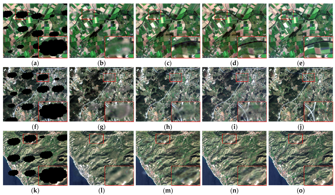
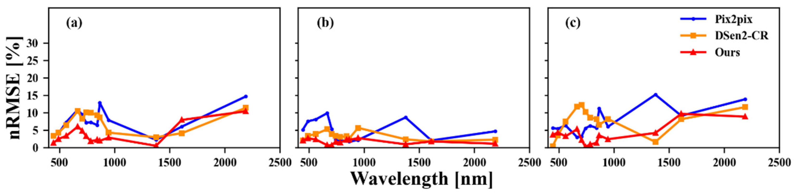
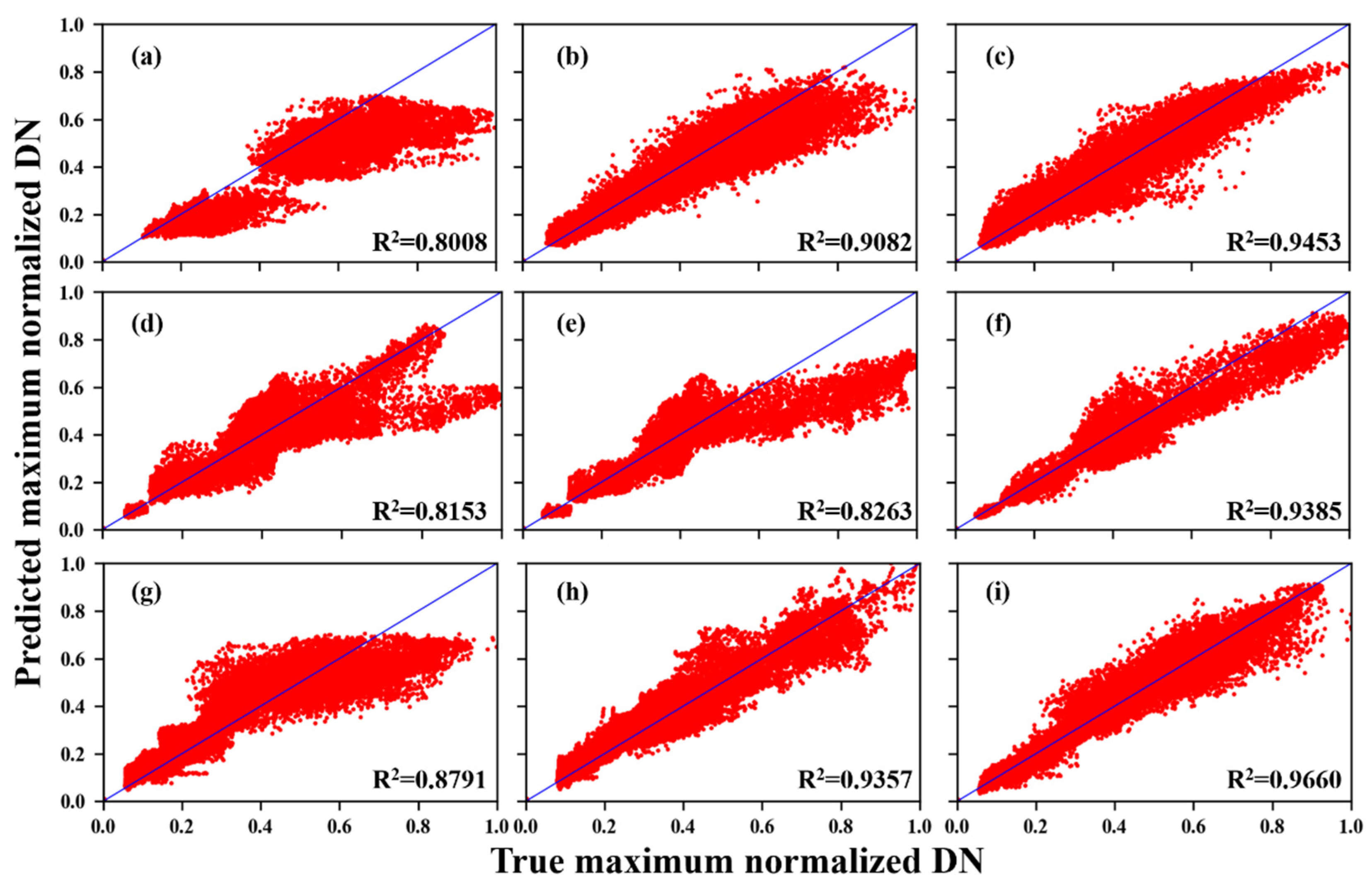
3.2. Simulated Data Experiments

To verify the proposed G-FAN method, two deep learning models, pix2pix GAN framework (Pix2pix) [46] and DSen2-CR [27], were executed as the baselines for comparison in the simulated corrupted image. Pix2pix has been adopted in previous studies on cloud removal [28,29]. Pix2pix can learn the mapping and transforming correlation from the inputs of 13-channel multi-spectral cloudy optical images and dual-polarimetric SAR patches to the output of 13-channel multi-spectral cloud-free optical images. The optimizer for Pix2pix is Adam, with a learning rate of 2×10⁻⁴ in the first 75 epochs, and gradually decaying to 0 in the last 25 epochs. DSen2-CR exploits deep residual neural networks and SAR-optical data fusion to remove thick clouds and cloud shadows in Sentinel-2 remote sensing images. The Adam algorithm was adopted for DSen2-CR. The learning rate was 7 × 10⁻⁵ for a batch size of 16. The sizes of feature patches in the G-FAN were, respectively, $C=13$, $W_p=7$, and $H_p=7$ in our experiments.

The simulation experiment results of cloud removal with SAR and optical remote sensing images by Pix2pix, DSen2-CR, and the proposed method are presented in Figure 7. Furthermore,

Table 1. Quantitative evaluation of the results of the simulated data experiment.

	PSNR↑	SSIM↑	CC↑	SAM (°)↓	MAE↓
Pix2pix	29.8322	0.8806	0.7605	8.8129	0.0249
DSen2-CR	31.5108	0.9048	0.8115	6.2634	0.0198
Our Model	35.5591	0.9261	0.8826	2.8895	0.0157

↑ means that a higher score indicates a better result, and ↓ means that a lower score indicates a better result.

lists the quantitative evaluation results, including PSNR, SSIM, CC, SAM, and MAE. The first column of Figure 7 shows the simulated corrupted optical image. The results of Pix2pix, DSen2-CR, and the proposed method are, respectively, listed in the second, third, and fourth columns of Figure 7. Ground truth images corresponding to the simulated cloudy images are displayed in the fifth column of Figure 7. From the visual evaluation, all of the methods achieved a satisfying optical representation of the land surface structure. In particular, large structures, such as mountains, rivers, roads, and large fields in an agricultural example scene, were correctly included in the predicted image. We then magnified some restored areas for further comparison. It can be seen that the proposed method outperforms Pix2pix and DSen2-CR in terms of texture information reconstruction and tiny ground object reconstruction. The main reason for this may be that our method fused the GFAM into the traditional residual architecture, by which similar non-local information of a long range is extracted and exploited to restore missing data. The spectral information of neighborhood pixels and non-neighborhood pixels, and electromagnetic backscattering information, were aggregated by the graph attention mechanism, enhancing the visual evaluation and quantitative evaluation of our results. Combined with the error analysis of the area boxed in red in Figure A1 and Figure A2, we can see that the predicted value of our method in the reconstructed region is closer to the true value than that of the others, and the 13-channel-wise normalized root mean square error (nRMSE) of our method was small in general. From the visual and quantitative analyses of the reconstruction results, it can be seen that the proposed G-FAN achieved the best results among all three methods in the simulated data experiments.

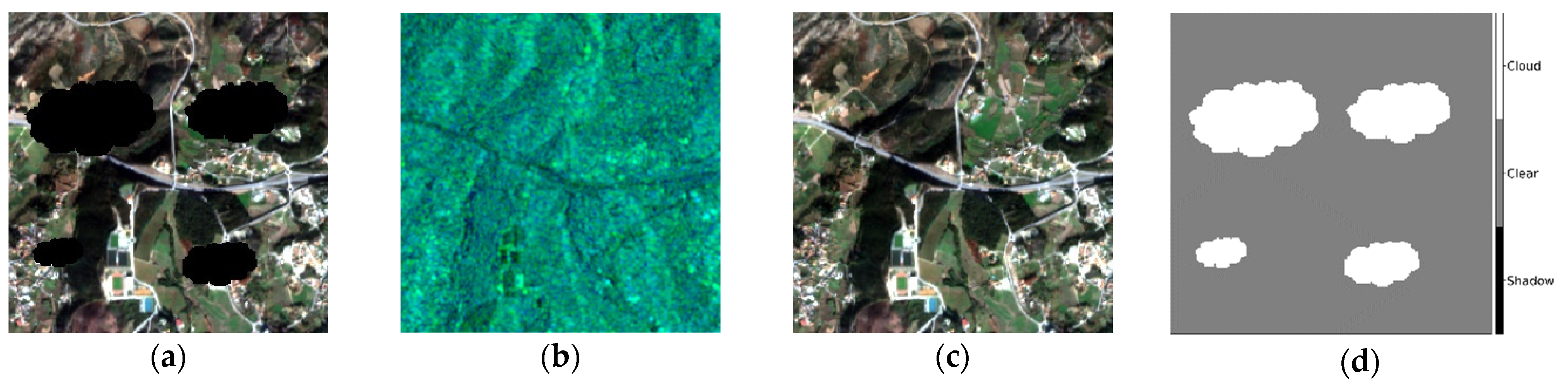
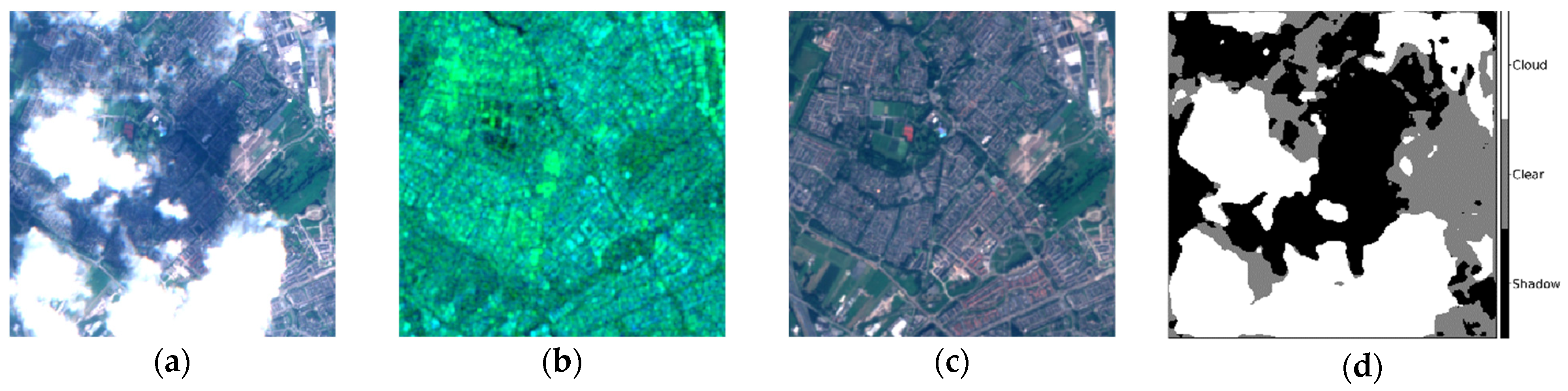
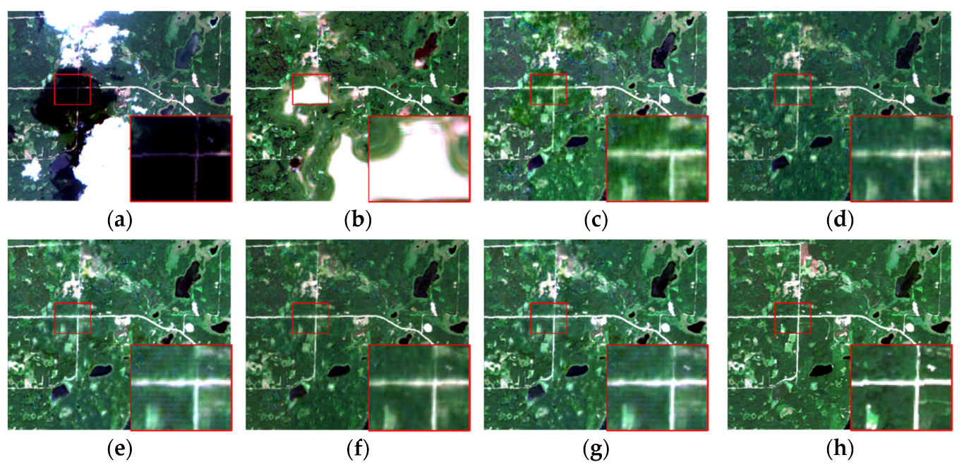
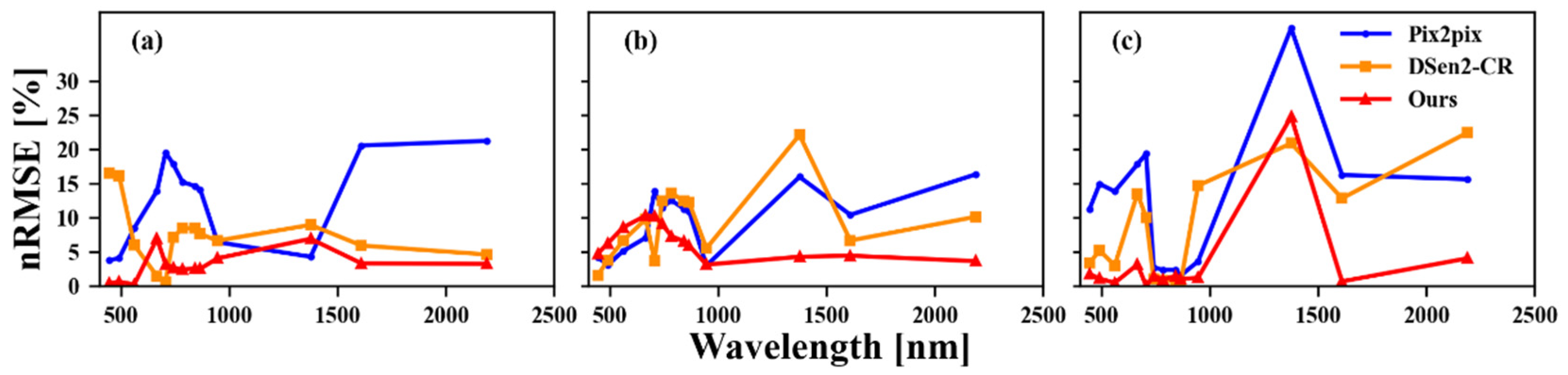
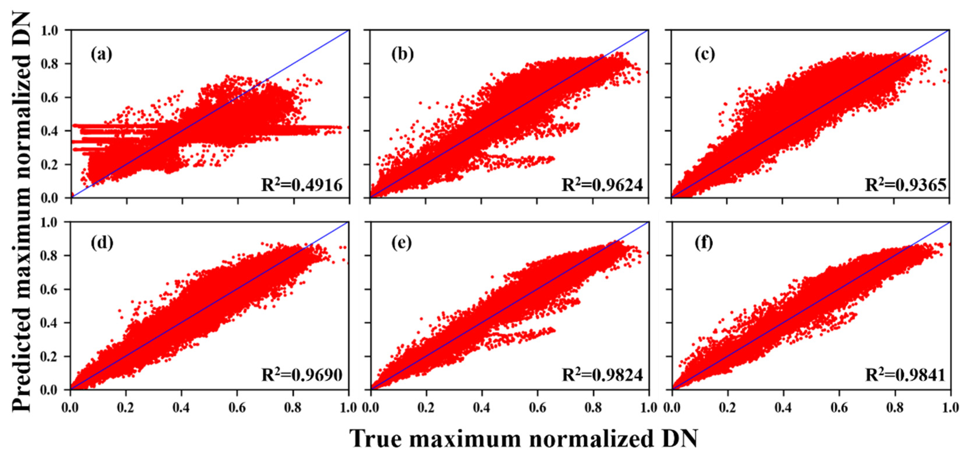
3.3. Real Data Experiments

To further demonstrate the merits of our proposed method, we applied it to the more challenging task of real, multi-spectral optical remote sensing images from the dataset introduced in [27]. Unlike simulated data experiments, in this case, the thick cloud and cloud shadow area of the cloudy optical images were detected and removed by the method introduced in Section 3.1.1. We compared our method with Pix2pix and DSen2-CR. The quantitative results are shown in

Table 2. Quantitative evaluation of the results of the real data experiment.

	PSNR↑	SSIM↑	CC↑	SAM (°)↓	MAE↓
Pix2pix	28.7996	0.8725	0.7504	11.6827	0.0277
DSen2-CR	30.1207	0.8930	0.8013	7.6163	0.0250
Our Model	34.4016	0.9164	0.8264	4.2715	0.0172

↑ means that a higher score indicates a better result, and ↓ means that a lower score indicates a better result.

, and we further provide a visual comparison of the different methods in Figure 8. The three methods, based on the deep learning model, make good use of electromagnetic backscattering information and spectral information of neighborhood pixels to reconstruct the missing data area contaminated by clouds, and the basic structure and basic feature information of the land surface can be well restored; however, the performances of the three methods regarding precision and tiny object restoration remain different. Moreover, the PSNR, SSIM, CC, SAM, and MAE values listed in Table 2 suggest that the proposed method outperforms Pix2pix and DSen2-CR. From Figure 8, it can be seen that the restoration results of the proposed method are generally better than those of the Pix2pix model and DSen2-CR model.

As is shown in the second column in Figure 8, the results generated by the Pix2pix model show a deviation of the spectral value from the ground truth. In contrast, DSen2-CR and the proposed model performed better in reconstructing the spectral information of the ground truth. The quantitative evaluation results listed in Table 2, and the error analysis of the area boxed in red in Figure A3 and Figure A4, confirm that the DSen2-CR and the proposed model could generate better results to some degree; moreover, the proposed model performed better than the other two models. In addition, the proposed model outperformed the other two models in terms of tiny ground object reconstruction. We observed that, as indicated by in the second, third, and fourth columns of Figure 8, the DSen2-CR model could not successfully restore some parts of built-up lands and croplands, which, in the figure, are boxed in red and magnified. Compared with ground truth, the results of the Pix2pix model exhibit a lack of contextual continuity in texture reconstruction, and more anomalous noise and a non-actual texture would be produced in some parts of the restored region. In contrast, the proposed model could precisely restore this tiny object. Furthermore, the quantitative error evaluation of the predicted value and the true value of the area boxed in red are shown in Figure A3 and Figure A4 in the form of scatter diagrams and channel-wise nRMSE. The scatter diagrams and their multi-channel error curve also imply the reconstruction precision of the proposed methods. In general, the proposed model shows its superiority in terms of spectral restoration and ground object reconstruction compared with the Pix2pix model and DSen2-CR model.

3.4. Ablation Experiments

To further verify the function of each piece of data and module in the proposed network, we performed some ablation experiments, and mainly analyzed the influence of SAR-optical data fusion, the number of residual blocks, the effect of M-GFAM, and the loss function in the proposed method. The quantitative results of the ablation experiments are shown in

Table 3. Quantitative evaluation of the results of the ablation experiments.

	PSNR↑	SSIM↑	CC↑	SAM (°)↓	MAE↓
w/o SAR	27.8501	0.8267	0.6840	9.6827	0.0296
8 Residual blocks (M-GFAM + 8 residual blocks + $L_{\mathrm{G}-\mathrm{FAN}}$)	28.6487	0.8627	0.7989	7.8166	0.0207
Single GFAM (Single GFAM + 16 residual blocks + $L_{\mathrm{G}-\mathrm{FAN}}$)	33.7955	0.8843	0.8147	5.0221	0.0195
Smooth L1 (M-GFAM + 16 residual blocks + Smooth L1)	34.2943	0.9047	0.8129	4.3182	0.0179
32 Residual blocks (M-GFAM + 32 residual blocks + $L_{\mathrm{G}-\mathrm{FAN}}$)	34.4770	0.9089	0.8295	4.2890	0.0168
Ours (M-GFAM + 16 residual blocks + $L_{\mathrm{G}-\mathrm{FAN}}$)	34.4016	0.9164	0.8264	4.2715	0.0172

↑ means that a higher score indicates a better result, and ↓ means that a lower score indicates a better result.

, and visual comparisons of different methods are shown in Figure 9. A more detailed analysis and discussion are provided in the following sections.

3.4.1. Effect of SAR-Optical Data Fusion

In the proposed method, the SAR image and the optical image are fused and inputted into a deep learning model for cloud removal, so the SAR information is important auxiliary information in the proposed model. In order to demonstrate the function of the SAR information, we conducted a cloud removal experiment without an SAR auxiliary input. As shown in Figure 9b, information of the land surface in the missing data region can hardly be reconstructed without an SAR image, except for some edge areas. This phenomenon may be due to a multi-level convolution in the residual module of our model extracting some neighborhood information of intact pixels. Some central areas away from the edge in the missing data region are filled with similar spectral values, which almost resembles an extension of the intact neighborhood pixels. This demonstrates that the model without an SAR auxiliary input can learn some basic reconstruction principles, such as filling or extension of neighborhood pixels, after many epochs of training. Combined with the scatter diagrams of the error analysis shown in Figure A5 for the area boxed in red, and the quantitative results in Table 3, it can clearly be seen that the model without an SAR auxiliary input obtained a poor reconstruction result in the cloud-contaminated area.

3.4.2. Performance with Different Numbers of Residual Blocks

To show the impact of our model structure, we tested the performance of our model with different numbers of residual blocks, so the new comparative models, respectively, contained eight residual blocks and 32 residual blocks in this ablation experiments, while other parts of the comparative models are the same as for our own. Figure 9c,f,g shows a visual effect of the results. The second, fifth, and sixth rows of Table 3 are the quantitative results. Figure A5b,e,f presents the scatter diagrams of the error analysis of the areas boxed in red in Figure 9c,f,g. Combining the figures and the table, we can see that the information extraction and precision in the missing data reconstruction became poorer with the decrease in residual blocks in our model. Some parts of the red boxed area in Figure 9c show color distortion and image blurring. However, from the overall visual perspective, the land surface structure of the cloud-contaminated region can achieve reasonable reconstruction by the models with eight residual blocks and 32 residual blocks, and this also demonstrates that the basic model and idea of the proposed method are feasible. Meanwhile, we can see that there is no significant improvement when the number of residual blocks increases from 16 to 32. Combined with the time costs exhibited in

Table 4. Time cost of three comparison methods and our method.

	Pix2pix	DSen2-CR	Ours	32 Residual Blocks
Time	0.14 s	0.22 s	0.32 s	0.41 s

, we found that the complexity of the network increased. Therefore, considering the precision of the reconstructed images and the complexity of the network, the proposed network with 16 residual blocks may be the best of the three comparative networks.

3.4.3. Effect of M-GFAM

In order to analyze the role of M-GFAM in our model, we conducted an ablation experiment. In this experiment, we reduced the number of GFAMs from four to one, so that M-GFAM in our model is transformed into a single GFAM. Meanwhile, the other parts of our model, such as residual blocks and loss function, remain unchanged. The quantitative results of the ablation experiments are shown in Table 3, the scatter diagrams for error analysis are shown in Figure A5c,f, and visual comparisons of different methods are shown in Figure 9d,g. In addition, our model is inspired by DSen2-CR, and we combined the ResNet and M-GFAM to construct the architecture of our model. Therefore, the DSen2-CR is similar to our model without GFAM. From the combined results of DSen2-CR in Section 3.3 and the supplementary ablation experiment, we can see that the proposed deep learning model with ResNet and M-GFAM outperforms the model without GFAM(DSen2-CR), as well as the model with a single GFAM, in the qualitative and quantitative evaluation.

3.4.4. Influence of Loss Function

We conducted an ablation study of our loss function. In this experiment, the model was only equipped with $L_{{\mathrm{Smooth} L}_1}$. Figure 9e shows some examples of the results with $L_{{\mathrm{Smooth} L}_1}$, while Figure 9g shows the results of the proposed method with $L_{\mathrm{G}-\mathrm{FAN}}$. Table 3 shows the quantitative results. Figure A5d,f presents the scatter diagrams of the error analyses of the area boxed in red in Figure 9e,g. Comparing the figures and table, one can see that the proposed model with $L_{\mathrm{G}-\mathrm{FAN}}$, which has a fused $L_{{\mathrm{Smooth} L}_1}$ and $L_{\mathrm{MS}-\mathrm{SSIM}}$, outperformed the model with $L_{{\mathrm{Smooth} L}_1}$ only, and some tiny ground objects and land surface structures were shown more distinctly in the results of the method with $L_{\mathrm{G}-\mathrm{FAN}}$ than that with $L_{{\mathrm{Smooth} L}_1}$. Furthermore, this demonstrates that the model equipped with a loss function with fused $L_{{\mathrm{Smooth} L}_1}$ and $L_{\mathrm{MS}-\mathrm{SSIM}}$ can improve the visual effects and enhance the SSIM.

4. Discussion

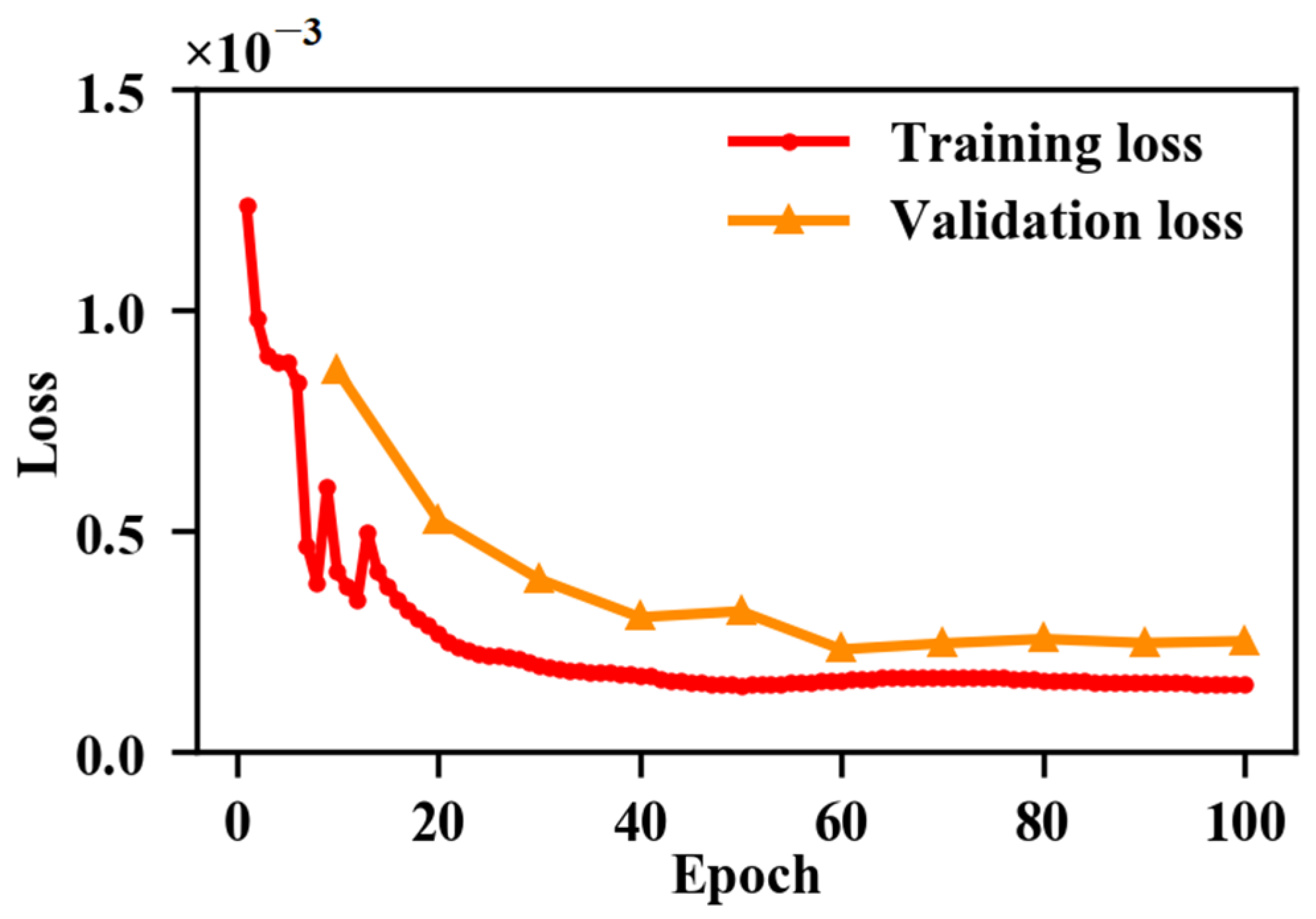
4.1. Overfitting Issues of Model

Overfitting is a common problem of the deep learning model in the training procedure. In order to check the overfitting issues of our model, we reviewed the final result and training loss of our model. Owing to a large training dataset we collected to train our network, and the gradual descent strategy of learning rate, the proposed model is not overfitted. From Figure 10, we can see that the convergence of losses for the training set and validation set is consistent. Nevertheless, the method used to alleviate the overfitting of deep learning models will be a focus in our future work.

4.2. Computation Complexity

Despite the fact that the proposed approach can take electromagnetic backscattering information and spectral information into consideration, and also obtain results with both good quantitative and qualitative evaluation, we have to admit that the above achievements are at the cost of efficiency. The proposed model is derived from ResNet for cloud removal, and we add M-GFAM in order to aggregate the similar non-local features in feature maps. Due to the utilization of the GCN principle and the attention mechanism, the computation complexity of our approach is higher than DSen2-CR and Pix2pix; however, the time cost of these methods is almost of the same order of magnitude, and it does not affect the usability of our method in practical applications. Table 4 lists the time costs of the proposed method and three comparison methods on the test sample, with a size of 256 × 256. Pix2pix takes the least time compared to DSen2-CR and our own model, because of its low computation complexity. The time cost of our model is higher than DSen2-CR, since the introduction of GFAMs to the cloud removal method induces additional computation. With an increase in residual blocks, the amount of computation will further increase. Therefore, we seek a solution for improving the efficiency of our method in future work.

4.3. Comparisons of Difference Cloud Detection Methods

In the procedure of cloud removal, cloud detection is the first step in cloud-contaminated pixel identification and masking. In order to analyze the influence of cloud detection methods, we conducted comparative real data experiments on cloud/cloud shadow detection methods [44,45] and F-mask [47,48]. The results are presented in

Table 5. Quantitative evaluation of our model with different cloud detection methods.

	PSNR↑	SSIM↑	CC↑	SAM (°)↓	MAE↓
F-mask [47,48] + G-FAN	34.5342	0.9033	0.8196	4.2487	0.0164
cloud/cloud shadow detection [44,45] + G-FAN(Our model)	34.4016	0.9164	0.8264	4.2715	0.0172

↑ means that a higher score indicates a better result, and ↓ means that a lower score indicates a better result.

. These results show that the quantitative evaluations of different cloud detection methods are similar. Owing to the large training dataset we adopted to train our network and the aggregation mechanism of similar non-local features, the effect of cloud detection on our model is small. According to the overall statistical results, the difference observed between the cloud detection methods may be reduced by applying the deep learning model and training with big data.

5. Conclusions

In this paper, we have present a novel cloud removal method using SAR-optical data fusion and a graph-based feature aggregation network for Sentinel-2 optical imagery. The proposed deep learning model can reconstruct the missing data region contaminated by clouds and cloud shadows based on the spectral information of the neighborhood pixels and the non-neighborhood pixels in optical images, as well as the electromagnetic backscattering information in SAR images. Since SAR images used as auxiliary data for cloud removal and image restoration may be blurred and noisy, the proposed G-FAN, which makes use of the advantages of the GAT, the feature aggregation mechanism, and residual connections, can achieve the simultaneous processing of cloud removal, image deblurring, and image denoising. A loss function based on the smooth L1 loss function and MS-SSIM is proposed and utilized in our model. Our loss function inherits the many advantages of the smooth L1 loss function and MS-SSIM, and obtains an effect suitable for human vision. Compared with other SAR- and optical image fusion-based cloud removal methods, our results show that the proposed G-FAN can achieve a significant improvement in terms of reconstruction accuracy and visual perception in both simulated data and real data experiments.

Although the proposed method can achieve a satisfactory reconstruction effect in terms of thick cloud and shadow removal, several issues must be considered. First, since only two bands of electromagnetic scattering coefficients are used in our model, the interpretability of SAR may be a limitation. Some specific backgrounds, such as urban and built-up lands with complicated patterns, cannot be identified precisely. Thus, in such cases, the network fails to provide a detailed and fully accurate reconstruction. In our future work, we will try to introduce multi-band SAR to enhance the interpretability of specific backgrounds with complicated patterns. Second, the early stopping technique is a good strategy to improve deep neural network training, and we would adopt this technique to increase the computational speed and reduce the overfitting issues in practical applications. Finally, thin cloud (such as smoke, haze), thick cloud, and cloud shadow regions will be separately reconstructed. Moreover, we will modify the network structure and expand the application to remote sensing image denoising and thin cloud removal in future research.

References

1. Zhang, B.; Wu, Y.; Zhao, B.; Chanussot, J.; Hong, D.; Yao, J.; Gao, L. Progress and challenges in intelligent remote sensing satellite systems. IEEE J. Sel. Top. Appl. Earth Obs. Remote Sens. 2022, 15, 1814–1822. [Google Scholar] [CrossRef]
2. Liu, Y.; Zuo, X.; Tian, J.; Li, S.; Cai, K.; Zhang, W. Research on generic optical remote sensing products: A review of scientific exploration, technology research, and engineering application. IEEE J. Sel. Top. Appl. Earth Obs. Remote Sens. 2021, 14, 3937–3953. [Google Scholar] [CrossRef]
3. Wang, S.; Li, J.; Zhang, B.; Lee, Z.; Spyrakos, E.; Feng, L.; Liu, C.; Zhao, H.; Wu, Y.; Zhu, L.; et al. Changes of water clarity in large lakes and reservoirs across China observed from long-term MODIS. Remote Sens. Environ. 2020, 247, 111949. [Google Scholar] [CrossRef]
4. Zhao, X.; Hong, D.; Gao, L.; Zhang, B.; Chanussot, J. Transferable deep learning from time series of Landsat data for national land-cover mapping with noisy labels: A case study of China. Remote Sens. 2021, 13, 4194. [Google Scholar] [CrossRef]
5. Youssefi, F.; Zoej, M.J.V.; Hanafi-Bojd, A.A.; Dariane, A.B.; Khaki, M.; Safdarinezhad, A.; Ghaderpour, E. Temporal monitoring and predicting of the abundance of malaria vectors using time series analysis of remote sensing data through Google Earth Engine. Sensors 2022, 22, 1942. [Google Scholar] [CrossRef]
6. Duan, C.; Pan, J.; Li, R. Thick cloud removal of remote sensing images using temporal smoothness and sparsity regularized tensor optimization. Remote Sens. 2020, 12, 3446. [Google Scholar] [CrossRef]
7. Xia, M.; Jia, K. Reconstructing missing information of remote sensing data contaminated by large and thick clouds based on an improved multitemporal dictionary learning method. IEEE Trans. Geosci. Remote Sens. 2022, 60, 5605914. [Google Scholar] [CrossRef]
8. Ju, J.; Roy, D.P. The availability of cloud-free landsat etm plus data over the conterminous United States and globally. Remote Sens. Environ. 2008, 112, 1196–1211. [Google Scholar] [CrossRef]
9. Liu, C.; Zhang, Y.; Chen, P.; Lai, C.; Chen, Y.; Cheng, J.; Ko, M. Clouds classification from Sentinel-2 imagery with deep residual learning and semantic image segmentation. Remote Sens. 2019, 11, 119. [Google Scholar] [CrossRef] [Green Version]
10. Jeppesen, J.H.; Jacobsen, R.H.; Inceoglu, F.; Toftgaard, T.S. A cloud detection algorithm for satellite imagery based on deep learning. Remote Sens. Environ. 2019, 229, 247–259. [Google Scholar] [CrossRef]
11. Sun, L.; Yang, X.; Jia, S.; Jia, C.; Wang, Q.; Liu, X.; Wei, J.; Zhou, X. Satellite data cloud detection using deep learning supported by hyperspectral data. Int. J. Remote Sens. 2019, 41, 1349–1371. [Google Scholar] [CrossRef] [Green Version]
12. Lu, C.; Xia, M.; Qian, M.; Chen, B. Dual-branch network for cloud and cloud shadow segmentation. IEEE Trans. Geosci. Remote Sens. 2022, 60, 5410012. [Google Scholar] [CrossRef]
13. Zhao, W.; Qu, Y.; Chen, J.; Yuan, Z. Deeply synergistic optical and SAR time series for crop dynamic monitoring. Remote Sens. Environ. 2020, 247, 111952. [Google Scholar] [CrossRef]
14. Santangelo, M.; Cardinali, M.; Bucci, F.; Fiorucci, F.; Mondini, A. Exploring event landslide mapping using Sentinel-1 SAR backscatter products. Geomorphology 2022, 397, 108021. [Google Scholar] [CrossRef]
15. Liu, Y.; Qian, J.; Yue, H. Combined Sentinel-1A with Sentinel-2A to estimate soil moisture in farmland. IEEE J. Sel. Top. Appl. Earth Obs. Remote Sens. 2021, 14, 1292–1310. [Google Scholar] [CrossRef]
16. Maalouf, A.; Carre, P.; Augereau, B.; Fernandez-Maloigne, C. A bandelet-based inpainting technique for clouds removal from remotely sensed images. IEEE Trans. Geosci. Remote Sens. 2009, 47, 2363–2371. [Google Scholar] [CrossRef]
17. Zheng, J.; Liu, X.; Wang, X. Single image cloud removal using U-Net and generative adversarial networks. IEEE Trans. Geosci. Remote Sens. 2021, 59, 6371–6384. [Google Scholar] [CrossRef]
18. Meng, F.; Yang, X.; Zhou, C.; Li, Z. A sparse dictionary learning-based adaptive patch inpainting method for thick clouds removal from high-spatial resolution remote sensing imagery. Sensors 2017, 17, 2130. [Google Scholar] [CrossRef] [Green Version]
19. Zhang, Y.; Wen, F.; Gao, Z.; Ling, X. A coarse-to-fine framework for cloud removal in remote sensing image sequence. IEEE Trans. Geosci. Remote Sens. 2019, 57, 5963–5974. [Google Scholar] [CrossRef]
20. Li, X.; Wang, L.; Cheng, Q.; Wu, P.; Gan, W.; Fang, L. Cloud removal in remote sensing images using nonnegative matrix factorization and error correction. ISPRS J. Photogramm. Remote Sens. 2019, 148, 103–113. [Google Scholar] [CrossRef]
21. Cao, R.; Chen, Y.; Chen, J.; Zhu, X.; Shen, M. Thick cloud removal in Landsat images based on autoregression of Landsat time-series data. Remote Sens. Environ. 2020, 249, 112001. [Google Scholar] [CrossRef]
22. Zhang, Q.; Yuan, Q.; Zeng, C.; Li, X.; Wei, Y. Missing data reconstruction in remote sensing image with a unified spatial–temporal–spectral deep convolutional neural network. IEEE Trans. Geosci. Remote Sens. 2018, 56, 4274–4288. [Google Scholar] [CrossRef] [Green Version]
23. Ji, S.; Dai, P.; Lu, M.; Zhang, Y. Simultaneous cloud detection and removal from bitemporal remote sensing images using cascade convolutional neural networks. IEEE Trans. Geosci. Remote Sens. 2020, 59, 732–748. [Google Scholar] [CrossRef]
24. Xu, M.; Deng, F.; Jia, S.; Jia, X.; Plaza, A. Attention mechanism-based generative adversarial networks for cloud removal in Landsat images. Remote Sens. Environ. 2022, 271, 112902. [Google Scholar] [CrossRef]
25. Shen, H.; Wu, J.; Cheng, Q.; Aihemaiti, M.; Zhang, C.; Li, Z. A spatiotemporal fusion based cloud removal method for remote sensing images with land cover changes. IEEE J. Sel. Top. Appl. Earth Obs. Remote Sens. 2019, 12, 862–874. [Google Scholar] [CrossRef]
26. Angel, Y.; Houborg, R.; McCabe, M.F. Reconstructing cloud contaminated pixels using spatiotemporal covariance functions and multitemporal hyperspectral imagery. Remote Sens. 2019, 11, 1145. [Google Scholar] [CrossRef] [Green Version]
27. Meraner, A.; Ebel, P.; Zhu, X.; Schmitt, M. Cloud removal in Sentinel-2 imagery using a deep residual neural network and SAR-optical data fusion. ISPRS J. Photogramm. Remote Sens. 2020, 166, 333–346. [Google Scholar] [CrossRef]
28. Grohnfeldt, C.; Schmitt, M.; Zhu, X. A conditional generative adversarial network to fuse Sar and multispectral optical data for cloud removal from Sentinel-2 images. In Proceedings of the IGARSS 2018—2018 IEEE International Geoscience and Remote Sensing Symposium, Valencia, Spain, 22–27 July 2018; pp. 1726–1729. [Google Scholar]
29. Bermudez, J.; Happ, P.; Oliveira, D.; Feitosa, R. Sar to optical image synthesis for cloud removal with generative adversarial networks. In Proceedings of the ISPRS Mid-Term Symposium Innovative Sensing—From Sensors to Methods and Applications, Karlsruhe, Germany, 10–12 October 2018; pp. 5–11. [Google Scholar]
30. Gao, J.; Yi, Y.; Wei, T.; Zhang, G. Sentinel-2 cloud removal considering ground changes by fusing multitemporal SAR and optical images. Remote Sens. 2021, 13, 3998. [Google Scholar] [CrossRef]
31. He, W.; Yokoya, N. Multi-temporal sentinel-1 and-2 data fusion for optical image simulation. ISPRS Int. J. Geo-Inf. 2018, 7, 389. [Google Scholar] [CrossRef] [Green Version]
32. Eckardt, R.; Berger, C.; Thiel, C.; Schmullius, C. Removal of optically thick clouds from multi-spectral satellite images using multi-frequency SAR data. Remote Sens. 2013, 5, 2973–3006. [Google Scholar] [CrossRef] [Green Version]
33. Velickovic, P.; Cucurull, G.; Casanova, A.; Romero, A.; Lio, P.; Bengio, Y. Graph attention networks. In Proceedings of the International Conference on Learning Representations (ICLR), Vancouver, BC, Canada, 21–25 May 2018; pp. 1243–1255. [Google Scholar]
34. Baroud, S.; Chokri, S.; Belhaous, S.; Mestari, M. A brief review of graph convolutional neural network based learning for classifying remote sensing images. Procedia Comput. Sci. 2021, 191, 349–354. [Google Scholar] [CrossRef]
35. Hong, D.; Yokoya, N.; Chanussot, J.; Zhu, X. CoSpace: Common subspace learning from hyperspectral-multispectral correspondences. IEEE Trans. Geosci. Remote Sens. 2019, 57, 4349–4359. [Google Scholar] [CrossRef] [Green Version]
36. Hong, D.; Yokoya, N.; Ge, N.; Chanussot, J.; Zhu, X. Learnable manifold alignment (LeMA): A semi-supervised cross-modality learning framework for land cover and land use classification. ISPRS J. Photogramm. Remote Sens. 2019, 147, 193–205. [Google Scholar] [CrossRef] [PubMed]
37. Hong, D.; Gao, L.; Yao, J.; Zhang, B.; Plaza, A.; Chanussot, J. Graph convolutional networks for hyperspectral image classification. IEEE Trans. Geosci. Remote Sens. 2020, 59, 5966–5978. [Google Scholar] [CrossRef]
38. Kipf, T.; Welling, M. Semi-supervised classification with graph convolutional networks. In Proceedings of the International Conference on Learning Representations (ICLR), Toulon, France, 24–26 April 2017; pp. 1–14. [Google Scholar]
39. Yang, Z.; Pan, D.; Shi, P. Joint image dehazing and super-resolution: Closed shared source residual attention fusion network. IEEE Access 2021, 9, 105477–105492. [Google Scholar] [CrossRef]
40. Valsesia, D.; Fracastoro, G.; Magli, E. Deep graph-convolutional image denoising. IEEE Trans. Image Process. 2020, 29, 8226–8237. [Google Scholar] [CrossRef]
41. Valsesia, D.; Fracastoro, G.; Magli, E. Image denoising with graph-convolutional neural networks. In Proceedings of the IEEE International Conference on Image Processing (ICIP), Taipei, China, 22–25 September 2019; pp. 2399–2403. [Google Scholar]
42. Yu, J.; Liu, M.; Feng, H.; Xu, Z.; Li, Q. Split-attention multiframe alignment network for image restoration. IEEE Access 2020, 8, 39254–39272. [Google Scholar] [CrossRef]
43. Zhao, H.; Gallo, O.; Frosio, I.; Kautz, J. Loss functions for image restoration with neural networks. IEEE Trans. Comput. Imaging 2017, 3, 47–57. [Google Scholar] [CrossRef]
44. Schmitt, M.; Hughes, L.; Qiu, C.; Zhu, X. Aggregating cloud-free Sentinel-2 images with Google Earth Engine. In Proceedings of the ISPRS Annals of the Photogrammetry, Remote Sensing and Spatial Information Sciences, Munich, Germany, 18–20 September 2019; pp. 145–152. [Google Scholar]
45. Zhai, H.; Zhang, H.; Zhang, L.; Li, P. Cloud/shadow detection based on spectral indices for multi/hyperspectral optical remote sensing imagery. ISPRS J. Photogramm. Remote Sens. 2018, 144, 235–253. [Google Scholar] [CrossRef]
46. Isola, P.; Zhu, J.; Zhou, T.; Efros, A. Image-to-image translation with conditional adversarial networks. In Proceedings of the 2017 IEEE Conference on Computer Vision and Pattern Recognition (CVPR), Honolulu, HI, USA, 21–26 July 2017; pp. 1125–1134. [Google Scholar]
47. Qiu, S.; Zhu, Z.; He, B. Fmask 4.0: Improved cloud and cloud shadow detection in Landsats 4-8 and Sentinel-2 imagery. Remote Sens. Environ. 2019, 231, 111205. [Google Scholar] [CrossRef]
48. Frantz, D.; Hab, E.; Uhl, A.; Stoffels, J.; Hill, J. Improvement of the Fmask algorithm for Sentinel-2 images: Separating clouds from bright surfaces based on parallax effects. Remote Sens. Environ. 2018, 215, 471–481. [Google Scholar] [CrossRef]
Figure 1. Architecture of the proposed G-FAN.
Remotesensing 14 03374 g001
Figure 2. The basic architecture of the residual module and residual blocks.
Remotesensing 14 03374 g002
Figure 3. Details of the function module and architecture of our proposed M-GFAM and GFAM.
Remotesensing 14 03374 g003
Figure 4. An example of missing data reconstruction based on non-local feature aggregation and the graph attention model.
Remotesensing 14 03374 g004
Figure 5. Examples of patch triplets from the dataset adopted in the simulated data experiment. (a) Simulated corrupted image of a cloud-contaminated image (R = b4, G = b3, B = b2); (b) SAR image (R = 0, G = HV, B = VV); (c) cloud-free image (R = b4, G = b3, B = b2); (d) cloud mask.
Remotesensing 14 03374 g005
Figure 6. Examples of patch triplets from the dataset adopted in the real data experiment. (a) Cloudy image (R = b4, G = b3, B = b2); (b) SAR image (R = 0, G = HV, B = VV); (c) cloud-free image (R = b4, G = b3, B = b2); (d) cloud and cloud shadow mask.
Remotesensing 14 03374 g006
Figure 7. Results of each method in the simulated data experiment. (a,f,k) Simulated corrupted image; (b,g,l) results of the Pix2pix model; (c,h,m) results of the DSen2-CR model; (d,i,n) results of the proposed model; (e,j,o) ground truth.
Remotesensing 14 03374 g007
Figure 8. Results of each method in the real data experiment. (a,f,k) Cloudy image; (b,g,l) results of the Pix2pix model; (c,h,m) results of the DSen2-CR model; (d,i,n) results of the proposed model; (e,j,o) ground truth.
Remotesensing 14 03374 g008
Figure 9. Results of the ablation experiments. (a) Cloudy image; (b) results of the model without SAR input; (c) results of the model with 8 residual blocks; (d) results of the model with single GFAM; (e) results of the model with the L Smooth   L 1 loss function; (f) results of the proposed model with 32 residual blocks; (g) results of the proposed model; (h) ground truth.
Remotesensing 14 03374 g009
Figure 10. The loss curves of training and validation.
Remotesensing 14 03374 g010