Retrieval of Fractional Snow Cover over High Mountain Asia Using 1 km and 5 km AVHRR/2 with Simulated Mid-Infrared Reflective Band

Abstract

Accurate long-term snow-covered-area mapping is essential for climate change studies and water resource management. The NOAA AVHRR/2 provides a unique data source for long-term, large-spatial-scale monitoring of snow-covered areas at a daily scale. However, the value of AVHRR/2 in mapping snow-covered areas is limited, due to its lack of a shortwave infrared band for snow/cloud discrimination. We simulated the reflectance in the 3.75 µm mid-infrared band with a radiative transfer model and then developed three fractional-snow-cover retrieval algorithms for AVHRR/2 imagery at 1 km and 5 km resolutions. These algorithms are based on the multiple endmember spectral mixture analysis algorithm (MESMA), snow index (SI) algorithm, and non-snow/snow two endmember model (TEM) algorithm. Evaluation and comparison of these algorithms were performed using 313 scenarios that referenced snow-cover maps from Landsat-5/TM imagery at 30 m resolution. For all the evaluation data, the MESMA algorithm outperformed the other two algorithms, with an overall accuracy of 0.84 (0.85) and an RMSE of 0.23 (0.21) at the 1 km (5 km) scale. Regarding the effect of land cover type, we found that the three AVHRR/2 fractional-snow-cover retrieval algorithms have good accuracy in bare land, grassland, and Himalayan areas; however, the accuracy decreases in forest areas due to the shading of snow by the canopy. Regarding the topographic effect, the accuracy evaluation indices showed a decreasing and then increasing trend as the elevation increased. The accuracy was worst in the 4000–5000 m range, which was due to the severe snow fragmentation in the High Mountain Asia region; the early AVHRR/2 sensors could not effectively monitor the snow cover in this region. In this study, by increasing the number of bands of AVHRR/2 1 km data for fractional-snow-cover retrieval, a good foundation for subsequent long time series kilometre- resolution snow-cover monitoring has been laid.

1. Introduction

Snow cover is the most active element of the cryosphere, and its distribution and change are important for the study of global climate change and the surface energy balance [1,2,3]. Snow cover has high albedo and low thermal conductivity and is therefore a critical component of surface energy balance and global climate change feedback [4]. Snow cover is an important indicator of climate change because it covers a wide area and is sensitive to temperature [5]. Approximately one third of the Earth’s land surface is covered with snow and glacier, while approximately one sixth of the population depends on snow and glacier for survival [6,7]. Therefore, methods for realizing the long time series monitoring of snow cover are particularly important.

Remote sensing allows for observations over long time periods and at large scales; it is an important technical tool for snow-cover monitoring. Snow has unique spectral characteristics in the visible and shortwave infrared bands that are easily distinguishable from other land features [8,9,10]. Using these spectral properties, the snow-covered area (SCA) can be effectively identified using multispectral sensors on board satellites, such as the Thematic Mapper (TM) on board Landsat–5, the Advanced Very High Resolution Radiometer (AVHRR) on board the National Oceanic and Atmospheric Administration (NOAA) satellites, and the Moderate Resolution Imaging Spectroradiometer (MODIS) on board Terra and Aqua [11,12]. Using these excellent sensors combined with the normalized difference snow index (NDSI), binary snow cover can be effectively estimated [13]. However, due to the high altitude and strong heterogeneity, the snow in High Mountain Asia region is thin and fragmented, which results in large errors when using only binary snow-cover estimation. Therefore, it is particularly important to obtain subpixel snow-cover information, known as fractional snow cover (FSC).

Scholars have conducted in-depth studies on fractional snow cover using several of the sensors mentioned above. These studies can be broadly classified as using the snow index algorithm [13,14], snow/no-snow reflectance interpolation algorithm [15], SCAmod algorithm [16,17], mixed pixel decomposition algorithm [18,19,20,21], and machine learning algorithms [22,23,24,25,26,27]. The snow index algorithm uses NDSI and fractional snow cover to establish a linear relationship. Its simplicity and efficiency have led to its adoption by MOD10A1 V5 [28,29]. However, this empirical relation algorithm is difficult to apply to different global land surfaces due to the complex changes in land cover types, the physical properties of snow cover, imaging geometric relations, and other factors [30]. The snow/no-snow reflectance interpolation algorithm [15] estimates fractional snow cover by linear interpolation between non-snow signals and pure snow signals. However, the accuracy is limited due to less dependent spectral information. The SCAmod algorithm [16,17,31] is designed for forested areas and introduces transmittance to compensate for the effect of the canopy. However, no-snow, pure snow reflectance, and canopy transmittance need to be calculated separately. The mixed pixel decomposition algorithm uses snow, soil/rock, and vegetation (with shadows) to perform a linear spectral mixture analysis of multiband reflectance. This algorithm has a solid physical foundation, but the computational efficiency is relatively low [20]. Machine learning algorithms use artificial neural network technology to express the linear and nonlinear relationships between multiband reflectance and snow cover under different ground and observation conditions. The algorithm is more accurate, but it relies on training datasets, which are less generalizable and cannot be extended to large regions.

NOAA/AVHRR has accumulated nearly 40 years of data and has been the only means of continuously monitoring snow cover on a large scale and over long periods of time. However, the AVHRR sensor bands are few and slightly coarse in resolution, especially the early AVHRR/2, which lacks the 1.6 μm band needed for distinguishing cloud and snow. This has led to relatively few snow studies being conducted, even though scholars know that the sensor data are valuable. Existing snow-cover products based on AVHRR data are binary; for example, the Japan Aerospace Exploration Agency (JAXA) recently issued the Northern Hemisphere long-term snow-cover extent (SCE) product JASMES [32], and Hao produced China’s long-term snow-cover extent (SCE) product NIEER [33]. Although many scholars have investigated fractional snow cover using AVHRR data, most of these studies remain at the algorithmic level. Slater [15] used AVHRR observations to estimate fractional snow cover using the difference in NDVI values between snow and non-snow areas in winter. Metsamaki [16,31] used a model of snow reflectance in forest areas, which was an improvement over the linear interpolation algorithm. Zhu [34] improved an automatic endmember extraction algorithm proposed by Shi [35], based on MODIS reflectivity imagery, and applied it to AVHRR/2 1 km data. This algorithm automatically selects endmembers from images using indices such as NDVI and NDSI and retrieves the fractional snow cover using a linear spectral mixture analysis algorithm. However, it uses only two bands and non-snow/snow endmembers to retrieve the fractional snow cover and is therefore still generally a linear interpolation algorithm.

In this study, we make some improvements to the above three AVHRR fractional-snow-cover retrieval algorithms and apply them to AVHRR data at 1 km and 5 km scales. The three algorithms in this study are the snow index algorithm (SI), the non-snow/snow two-endmember model algorithm (TEM), and the multiple endmember spectral mixture analysis algorithm based on automatic endmember extraction (MEAMA) algorithm. Then, the high-spatial-resolution Landsat-5 data are used as the “ground truth”, to evaluate the accuracy. Our study optimizes the valuable data accumulated by the early AVHRR/2 and provides a reference for those who wish to use the data for fractional-snow-cover retrieval studies in the future.

2. Study Areas and Data Sources

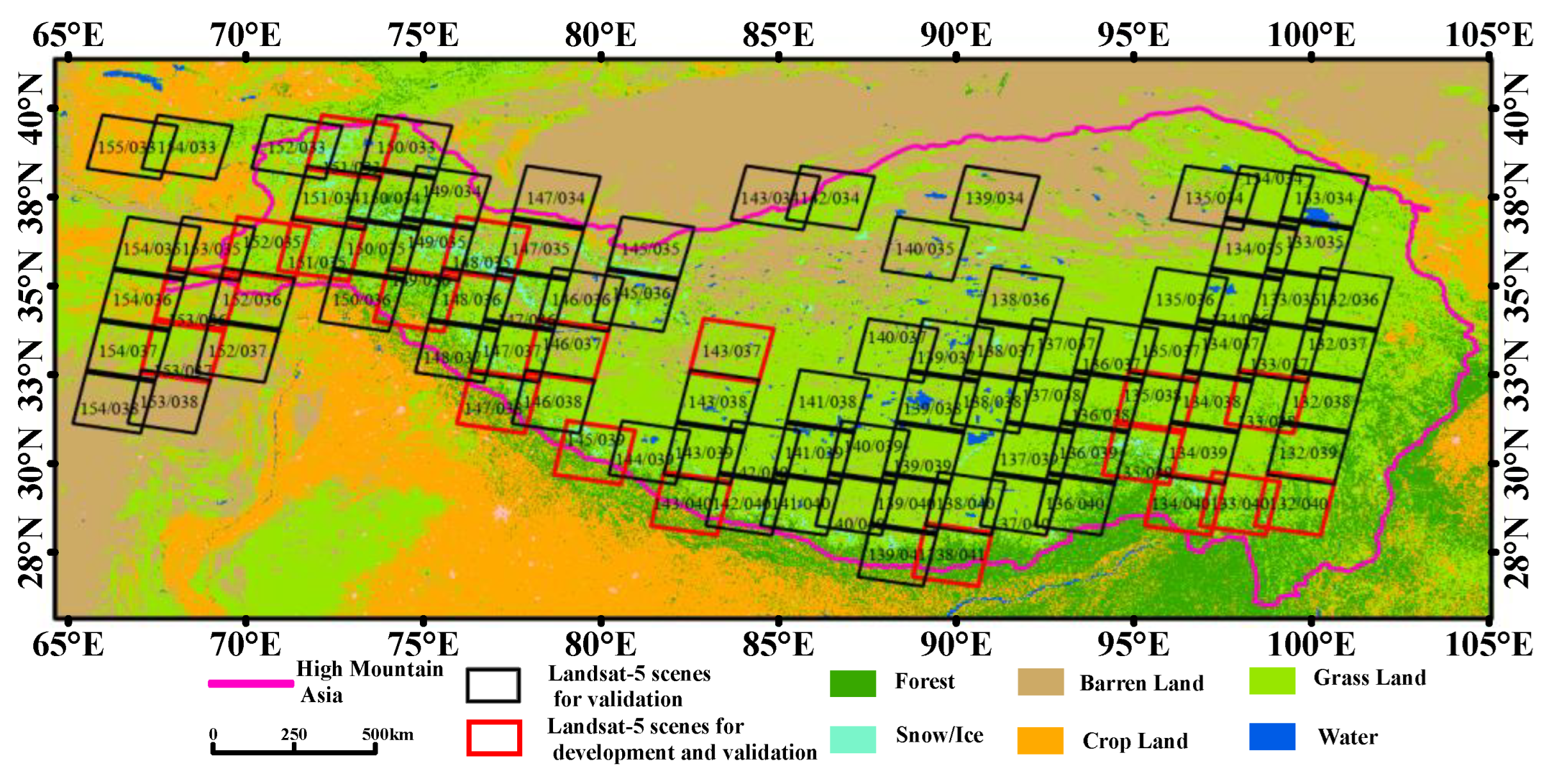
2.1. Study Areas

High Mountain Asia is a large tectonic geomorphic unit with the highest elevation in the world, and its snow and ice reserves are the largest outside the North and South Poles [36]. With a geographical range of approximately 24–40°N and 65–105°E [37], High Mountain Asia encompasses a cold and dry environment. The vector data used in this study were provided by the National Tibetan Plateau Data Center (http://data.tpdc.ac.cn (accessed on 15 March 2022)) (see Figure 1). The north and south boundaries of the range are determined by the northern foot of the West Kunlun-Qilian Mountains in the north and the southern foot of the Himalayas and other mountain ranges in the south, with a maximum width of 1560 km. The west and east boundaries of the range are determined by the western edge of the Hindu Kush and Pamir Plateau in the west and the eastern edge of the Hengduan Mountains and other mountain ranges in the east, with a maximum length of approximately 3360 km.

The terrain heterogeneity of the Tibetan Plateau varies substantially. Due to the strong influence of its topography and other factors, the snow cover in High Mountain Asia presents a large-patch distribution. Snow is more abundant at the periphery of High Mountain Asia and in the mountains. Snow is less abundant in the hinterland, basins, and valleys. The snow cover and its duration over High Mountain Asia have a significant influence on the atmospheric circulation at the local or hemispheric scale. In addition, its pre-eminence is a major feature of climate change over High Mountain Asia. Due to the impact of global warming, strengthening the research on High Mountain Asia snow cover and its surrounding areas is of great significance.

2.2. Advanced Very High Resolution Radiometer (AVHRR) Data

The data used in this study were acquired from an AVHRR sensor carried on board the NOAA series of meteorological satellites. The AVHRR sensors of the NOAA series satellites have been continuously conducting Earth observation missions since the launch of the TIROS-N satellite in 1979. The original satellite resolution for AVHRR data is 1 km, and these data are received and stored by satellite ground receiving stations around the world. NOAA resamples the data to 5 km to simplify data transmission, then following a series of pre-processing steps, the AVH09C1 5 km data are obtained. Subsequent studies that use AVHRR are based on 5 km data. The AVHRR sensor used in this study is an early generation 2 sensor named AVHRR/2. To evaluate the scale effects on the three fractional-snow-cover retrieval algorithms, both 1 km and 5 km resolution data are used in this study. The 1 km resolution data are the top-of-atmosphere (TOA) reflectivity data, and the 5 km resolution data are the surface reflectivity (SR) data. The three time periods for the data are November 1992 to March 1993, October 1995 to February 1996, and October 1996 to February 1997. The waveband settings are shown in

Table 1. AVHRR/2 characteristics.

Band Number	Spectral Range (μm)	Central Wavelength (μm)	Spatial Resolution (km)
1	0.55–0.68	0.615	1/5
2	0.725–1.1	0.912	1/5
3	3.55–3.93	3.75	1
4	10.3–11.3	10.80	1/5
5	11.5–12.5	12.00	1/5

below.

The 1 km resolution data of AVHRR/2 used in this study are the L1b-level data acquired and pre-processed by the National Satellite Meteorological Center of the China Meteorological Administration (http://data.nsmc.org.cn/(accessed on 5 March 2022)). The dataset contains top-of-atmosphere (TOA) reflectivity data in the 1 and 2 bands and brightness temperature data in the 3, 4, and 5 bands. Due to the lack of reflectivity data in the 3.75 μm band, the radiative transfer model combined with the brightness temperature of the 3 and 4 bands is used to estimate the reflectivity of the 3.75 μm band. Additionally, this study uses the FLAASH atmospheric correction plug-in of the ENVI software from ERSI to obtain the surface reflectance data for each reflectance band.

The 5 km resolution data of AVHRR/2 used in this study were taken from the AVH09C1 surface reflectance value product produced by NASA’s Long-Term Data Record team (https://ladsweb.modaps.eosdis.nasa.gov/ (accessed on 17 May 2021)). The latest version of AVH09C1 is V5, which employs subsequent atmospheric correction, satellite drift correction, and sensor radiation correction. The product has a spatial resolution of 5 km and a temporal resolution of 1 day. It contains surface reflectivity data in the 1, 2, and 3 bands and brightness temperature data in the 3, 4, and 5 bands and the QA band.

2.3. Landsat 4/5 Thematic Mapper (TM) Data

The Landsat 5 satellite, launched in 1984 by the United States, carries two main sensors: the Multispectral Scanner (MSS) and the Thematic Mapper (TM). Landsat 5’s satellite data have undergone a rigorous calibration process. The TM sensor passively senses solar radiation reflected from the Earth’s surface and radiated thermal radiation; it has seven bands covering a range of wavelengths from the visible to the infrared.

Table 2. Landsat-5/TM characteristics.

Band Number	Spectral Range (μm)	Central Wavelength (μm)	Spatial Resolution (km)
1	0.45–0.52	0.48	30 m
2	0.52–0.60	0.56	30 m
3	0.63–0.69	0.66	30 m
4	0.76–0.90	0.83	30 m
5	1.55–1.75	1.65	30 m
6	10.4–12.5	11.45	120 m
7	2.08–2.35	2.20	30 m

shows the settings of the Landsat-5/TM band. Landsat-5/TM data have a spatial resolution of 30 m and a temporal resolution of 16 days. Landsat-5/TM data are produced by the US Geological Survey (USGS) and are available for free download worldwide (https://Earthexplorer.usgs.gov (accessed on 5 March 2022)). The Landsat-5/TM atmospherically corrected surface reflectance product is used in this study. The Landsat-5/TM fractional snow cover is calculated using the MESMA algorithm and is used as “ground truth” data to validate the AVHRR/2 fractional-snow-cover retrieval results. The total number of Landsat 5/TM images used for validation in this study was 313 scenes.

2.4. Auxiliary Data

To better evaluate the accuracy of the three fractional-snow-cover retrieval algorithms at different spatial scales, some auxiliary types of information such as elevation data, surface classification data, and spectral library information regarding typical features are also used in this study. The elevation data used in this study are Shuttle Radar Topography Mission (SRTM) digital elevation model (DEM) data (http://srtm.csi.cgiar.org (accessed on 15 October 2021)) [38], which have a spatial resolution of 30 m and are mainly used to correct for topographic effects on the fractional-snow-cover retrieval of Landsat-5/TM data. The land use/land cover (LULC) data derived from the 30 m Thematic Mapper (TM) imagery classification were downloaded from the Data Center for Resources and Environmental Sciences, Chinese Academy of Sciences (http://www.resdc.cn/ (accessed on 15 October 2021)). Its land cover types were further reduced to six categories [39]. The accuracy of fractional-snow-cover retrieval results under different land surfaces was classified and evaluated according to the classification results. Spectral library information used in this study was obtained from the Johns Hopkins University spectral library (http://speclib.jpl.nasa.gov (accessed on 15 October 2021)) [40].

3. Methodology

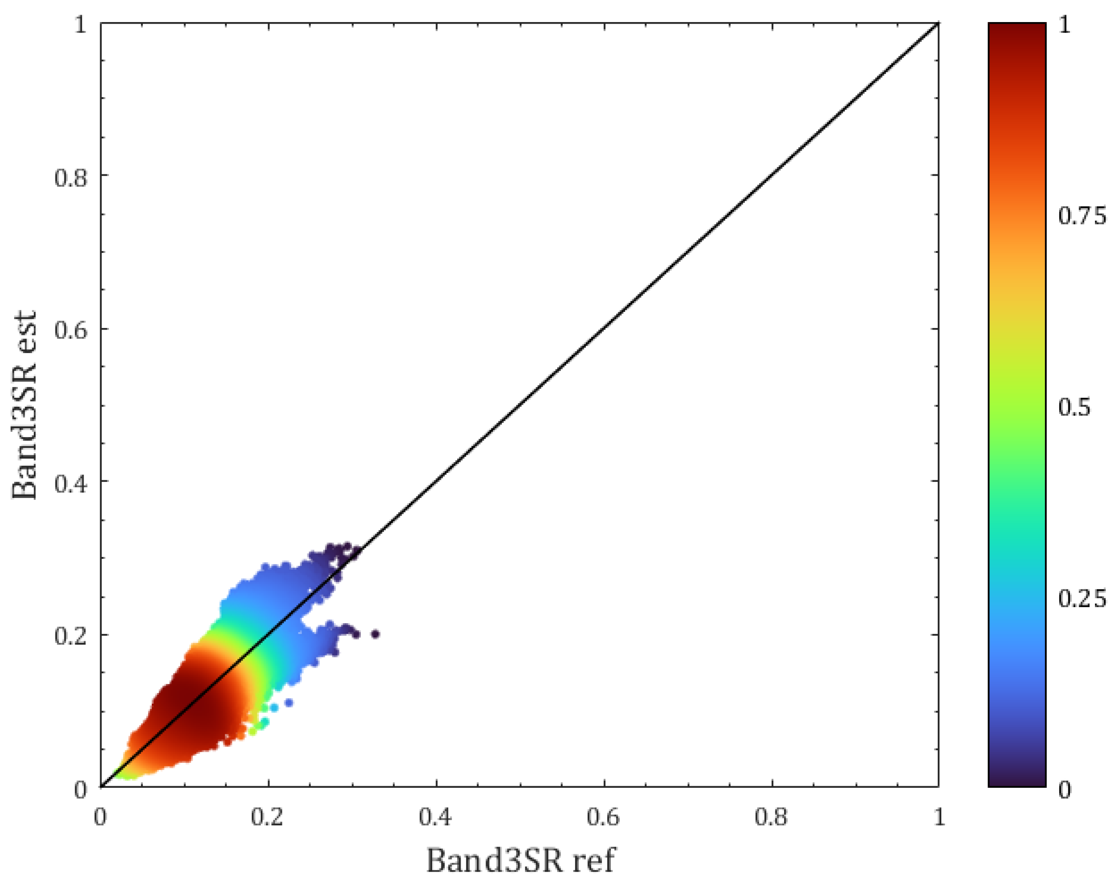
3.1. Simulated 3.75 μm Band Reflectance of AVHRR/2 1 km Data

Compared to other land feature classes such as clouds, etc., snow has unique spectral characteristics. Generally, snow exhibits a high reflectance in the visible band (0.6 μm) and a low reflectance in the shortwave infrared band (1.6 μm) and mid-infrared band (3.75 μm), resulting in its unique spectral characteristics. The 1.6 μm band is extremely important for the current snow-cover discrimination algorithm because, together with the 0.6 μm band, it typically forms the normalized difference snow index (NDSI), which can effectively distinguish snow from other land types and clouds. However, the AVHRR/2 sensor carried by the NOAA satellite lacks the 1.6 μm band, thereby negating the ability of the sensor to directly use the NDSI index for the fractional-snow-cover retrieval algorithm.

The AVHRR/2 data do not contain the 1.6 μm band, which is commonly used in fractional-snow-cover retrieval algorithms. Therefore, the mid-infrared band at 3.75 μm was used in this study instead. The radiation in the mid-infrared 3.75 μm band contains the target’s own emission and the reflection of solar radiation [41]. Hence, when calculating the reflectivity of the 3.75 μm band, the calculations for the emitted and reflected radiation in this band must be separated. In this study, we used the radiative transfer method to extract the reflectance in the mid-infrared 3.75 μm band with reference to the 5 km resolution product. The method mainly uses the brightness temperature of the 10.8 μm and 3.75 μm bands to obtain the reflectance of the 3.75 μm band through the radiative transfer equation. The specific calculation method is shown in Equations (1) and (2), where SR_3.75 denotes the spectral reflectance of the 3.75 μm band and BT_10.8 and BT_3.75 denote the brightness temperatures of the 10.8 μm and 3.75 μm bands, respectively. In addition, f(λ) refers to the spectral response function in the 3.75 μm band, s(λ) denotes the standard solar flux, and 𝜃 is the solar zenith angle. In the calculation, if BT_3.75 ≥ BT_10.8, Equation (1) is used to calculate BT_3.75, and when BT_3.75 < BT_10.8, Equation (2) is used.

$$S{R}_{3.75}=\frac{({\displaystyle {\int }_{3.55}^{3.93}Planck(B{T}_{3.75},\lambda )}f(\lambda )d\lambda -{\displaystyle {\int }_{3.55}^{3.93}Planck(B{T}_{10.8},\lambda )}f(\lambda )d\lambda )}{\cos \theta ({\displaystyle {\int }_{3.55}^{3.93}s(\lambda )}f(\lambda )d\lambda -{\displaystyle {\int }_{3.55}^{3.93}Planck(B{T}_{10.8},\lambda )}f(\lambda )d\lambda )}$$

(1)

$$S{R}_{3.75}=\frac{({\displaystyle {\int }_{3.55}^{3.93}Planck(B{T}_{3.75},\lambda )}f(\lambda )d\lambda -{\displaystyle {\int }_{3.55}^{3.93}Planck(B{T}_{10.8},\lambda )}f(\lambda )d\lambda )}{{\displaystyle {\int }_{3.55}^{3.93}Planck(B{T}_{10.8},\lambda )}f(\lambda )d\lambda }$$

(2)

We applied this algorithm to the AVH09C1 product to test its effectiveness. The brightness temperatures of the 10.8 μm and 3.75 μm bands were used to calculate the reflectance of the 3.75 μm band. Since the AVHRR/2 5 km data have reflectivity in the 3.75 μm band, this algorithm was applied to the AVHRR/2 5 km data to test its effectiveness. In this study, the calculated reflectances of the 3.75 µm band for 59 days from January to February 1993 were selected for comparison with the mean value of the reflectance of the official products in this band. The results are shown in Figure 2. The results indicate that the correlation between the two is very good, which proves the effectiveness of the algorithm.

3.2. Snow Index (SI) Algorithm

The snow index algorithm is used to establish a linear relationship between the snow index and fractional snow cover throughout the sample area, and then the relationship is further applied to the whole research area. For example, Kaufman developed a retrieval relationship for fractional snow cover based on reflectance in the 0.66 μm and 2.1 μm bands [42]. Due to the limitations of NDSI for fractional-snow-cover retrieval in forested areas and the fact that previous relational equations did not select training samples in the High Mountain Asia region, Wang (2021) constructed a combination of Universal Ratio Snow Index (URSI) and NDSI indices to develop a dynamic linear empirical relational equation applicable to the Tibetan Plateau region [30]. Salomonson and Appel used MODIS and Landsat ETM+ data to establish a regression relationship between MODIS NDSI values and fractional snow cover and applied this relationship to the previous version of the official MODIS fractional-snow-cover product [13,14].

However, most of the existing studies are based on MODIS data and Landsat TM/ETM+/OLI data, in which the lack of a 1.6 µm band in AVHRR/2 generation prevents the construction of the traditional snow index form, resulting in difficulties in applying this method. In this study, we constructed the snow index (SI) using the visible band and the 3.75 µm band of AVHRR/2 and then selected sample areas to establish the linear relationship between SI and fractional snow cover using Landsat-5/TM and AVHRR/2 data. The locations of the sample areas are shown in Figure 1. Equation (3) shows the formula for calculating the AVHRR/2 snow index. In this study, relationships were constructed using 1 km and 5 km resolution data: Equation (4) is the empirical relationship equation constructed at the 1 km scale, and Equation (5) is the empirical relationship equation constructed at the 5 km scale.

$$SI=\frac{S{R}_{VIS}-S{R}_{MIR}}{S{R}_{VIS}+S{R}_{MIR}}$$

(3)

$$FSC=1.95\times SI-0.12$$

(4)

$$FSC=1.25\times SI-0.05$$

(5)

where SI is the snow index of AVHRR/2, SR_VIS is the reflectance in the visible band, SR_MIR is the reflectance in the mid-infrared band, and FSC is the fractional snow cover of AVHRR/2.

3.3. Non-Snow/Snow Two Endmember Model (TEM) Algorithm

This method refers to the work of Wang [43] and Yang [44] on fractional-snow-cover retrieval using the FY-2E/F VISSR sensor, using a non-snow/snow two-endmember model, where the fractional snow cover is a linear interpolation of the snow endmember and non-snow endmember in the visible wavelength band. Because the FY-2E/F VISSR sensor has only one visible band, Wang also calculated the reflectivity of the mid-infrared band using brightness temperatures in the mid-infrared band (3.5–4.0 µm) and the infrared band (10.3–11.3 µm). Then, the fractional-snow-cover retrieval results of the FY-2E/F VISSR sensor can be obtained by using the non-snow/snow two-endmember model algorithm. The AVHRR/2 sensor band setting used in this study is similar to that of the FY-2E/F VISSR sensor, with an additional near-infrared band, so there is no theoretical barrier to porting this algorithm. The algorithm has the same selection rules for snow endmembers and non-snow endmembers under different ground classes, except that the thresholds for each rule are tailored according to the characteristics of the AVHRR/2 sensor.

Table 3. AVHRR/2 TEM algorithm endmember extraction rules.

Endmember	Rule for 1 km Data	Rule For 5 km Data
Full snow cover	SI > 0.70	SI > 0.75
	RVIS > 0.2 for forest	RVIS > 0.5 for forest
	RVIS > 0.25 for other land cover	RVIS > 0.6 for other land cover
Snow-free	SI < 0.50,	SI < 0.50,
	RVIS < 0.2 for grass and crop	RVIS < 0.5 for grass and crop
	RVIS < 0.25 for barren and forest	RVIS < 0.6 for barren and forest

below shows the selection rules for snow and non-snow endmembers across AVHRR/2 categories.

3.4. Multiple Endmember Spectral Mixture Analysis Algorithm Based on the Automatic Endmember Extraction (MESMA) Algorithm

Linear spectral mixing analysis is a commonly used spectral mixing model [45,46,47] that is suitable for alpine areas with low vegetation cover and a large optical thickness of snow [18,19]. The linear spectral mixture analysis model can be expressed by Equation (6), where the number of endmembers is less than the number of bands, and the result is the area ratio or abundance of each endmember via a least squares solution. In particular, to ensure the physical significance of the abundance, this ratio can be obtained using the fully constrained least squares method [42], as shown in Equations (7) and (8).

$$R_{\lambda }={\displaystyle \sum _{i=1}^N{F}_i{R}_{i,\lambda }+{\epsilon }_{\lambda }}$$

(6)

$${\displaystyle \sum _{i=1}^N{F}_i=1}$$

(7)

$$F_i\ge 0$$

(8)

where 𝐹_𝑖 is the area fraction of endmember i with reflectance 𝑅_𝑖,𝜆 at wavelength λ, N is the number of endmembers, 𝑅_𝜆 is the mixed pixel’s reflectance, and ε_λ is the residual error.

The MESMA method is a highly accurate method for estimating fractional snow cover in MODIS [30,33,34], which selects vegetation and soil/rock endmembers from the spectral database obtained from laboratory and field measurements and extracts snow endmembers with different grain sizes and incident–observation geometries using radiative transfer models. This algorithm uses the multi-endmember spectral mixture analysis method to calculate the fractional snow cover, which has high precision but requires many computations. Shi [35] proposed an automatic endmember extraction algorithm based on MODIS reflectivity images, which automatically selects endmembers from images using NDVI, NDSI, and other indices. Zhu [34] improved this method by using typical or neighbouring endmembers and solving them according to a two-endmember hybrid analysis model to achieve faster, high-precision, automated fractional-snow-cover calculation. Since the AVHRR/2 1 km data did not have reflectivity data in the 3.75 µm band, Zhu [30] could use only the two-endmember hybrid analysis model. In this study, the 3.75 µm band reflectance is calculated and combined with the reflectance of visible and near-infrared bands to select three typical endmembers of snow, vegetation, and bare land. In this study, various endmember extraction rules were adjusted for the characteristics of AVHRR/2 data with different spatial resolutions, as shown in

Table 4. AVHRR/2 MESMA algorithm endmember extraction rules.

Endmember	Rule For 1 Km Data	Rule For 5 Km Data
Snow	NDSI > 0.8 & NDVI < 0.05 & RVIS > 0.35	NDSI > 0.8 & NDVI < 0.2 & RVIS > 0.65
Vegetation	NDSI < 0.5 & NDVI > 0.1	NDSI < 0.2 & NDVI > 0.15
Bare land	NDSI < 0.3 & −0.15 < NDVI < 0	NDSI < 0.3 & −0.15 < NDVI < 0.1

below.

3.5. Evaluation Metrics

To quantitatively evaluate the accuracy of the three fractional-snow-cover retrieval algorithms at various spatial scales, in this study, we first aggregated the Landsat-5/TM fractional-snow-cover retrieval results based on the MESMA algorithm at a 30 m resolution to the corresponding spatial scales. Then, we selected three evaluation metrics: the overall accuracy (OA), the root mean square error (RMSE), and the coefficient of determination (R²), to evaluate the accuracy of the three fractional-snow-cover retrieval algorithms at different scales. The evaluation metrics are defined as follows:

$$OA=\frac{TP+TN}{TP+TN+FP+FN}$$

(9)

$$RMSE=\sqrt{\frac{1}{N}{\displaystyle \sum _N{(FS{C}_{AVHRR/2}-FS{C}_{Landsat-5/TM})}^2}}$$

(10)

$$R^2=\frac{[{\displaystyle \sum (FS{C}_{AVHRR/2}}-\overline{FS{C}_{AVHRR/2}})(FS{C}_{Landsat-5/TM}-\overline{FS{C}_{Landsat-5/TM}}){]}^2}{{\displaystyle \sum {(FS{C}_{AVHRR/2}-\overline{FS{C}_{AVHRR/2}})}^2{\displaystyle \sum {(FS{C}_{Landsat-5/TM}-\overline{FS{C}_{Landsat-5/TM}})}^2}}}$$

(11)

where TP indicates true positives, TN indicates true negatives, FP indicates false positives, FN indicates false negatives, FSC_AVHRR/2 indicates the fractional snow cover derived from the AVHRR/2 data, and FSC_Landsat-5/TM similarly indicates the fractional snow cover derived from the Landsat-5/TM data.

4. Results

To quantitatively evaluate the accuracy of the three AVHRR/2 fractional-snow-cover retrieval algorithms at different spatial scales, a total of 313 Landsat-5 images were selected as “ground truth” in this study for validation during the three winters. To better verify the accuracy of the three AVHRR/2 fractional-snow-cover retrieval algorithms, the selection rules for Landsat-5 images were as follows. QA marks of Landsat-5 images were used to select cloud cover less than 10%. According to the retrieval results, images with a snow-cover area accounting for more than 30% of the whole image were retained. To better evaluate the sensitivity of the three AVHRR/2 fractional-snow-cover retrieval algorithms to the surface types, we quantitatively evaluated the four surface type categories: bare ground, grassland, forest, and Himalayan region. Additionally, the results of the 1 km fractional-snow-cover retrieval were aggregated to the 5 km scale to investigate the influence of the observed scale on the fractional-snow-cover retrieval algorithm.

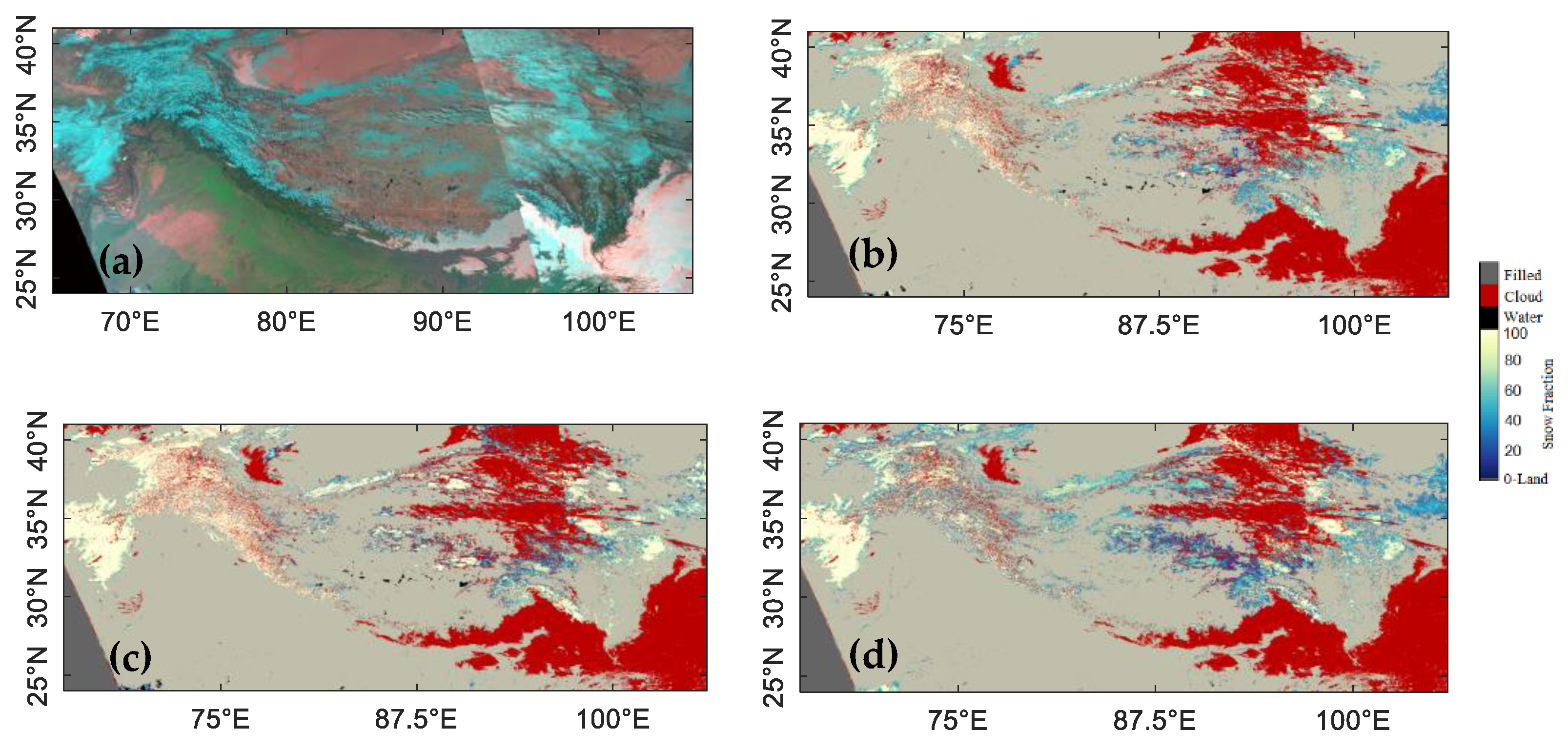
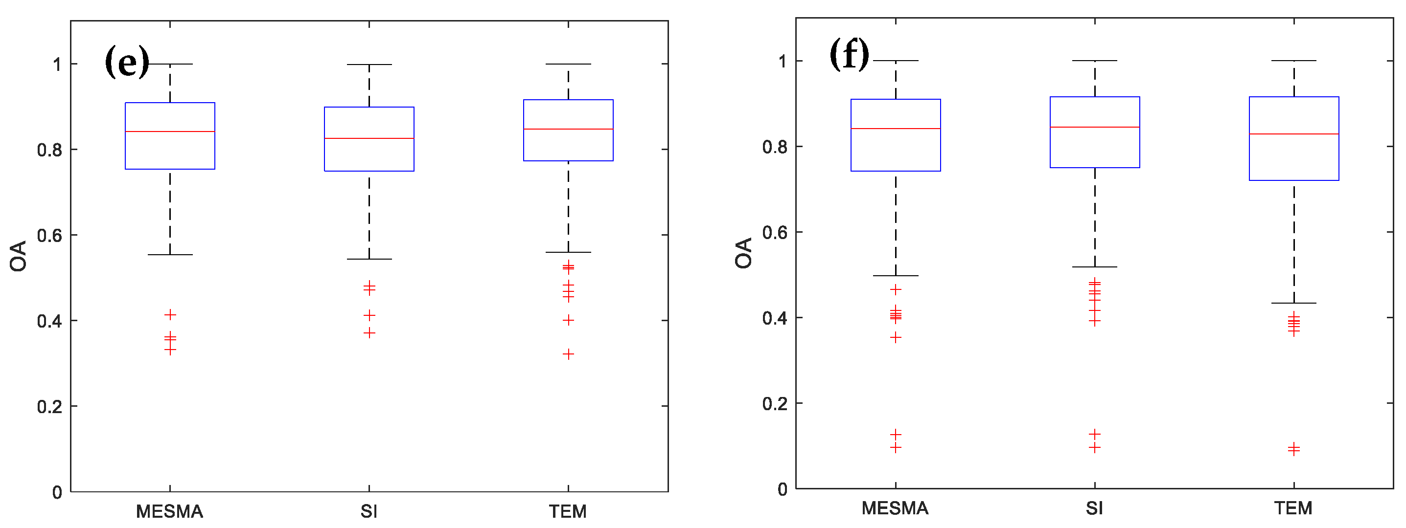
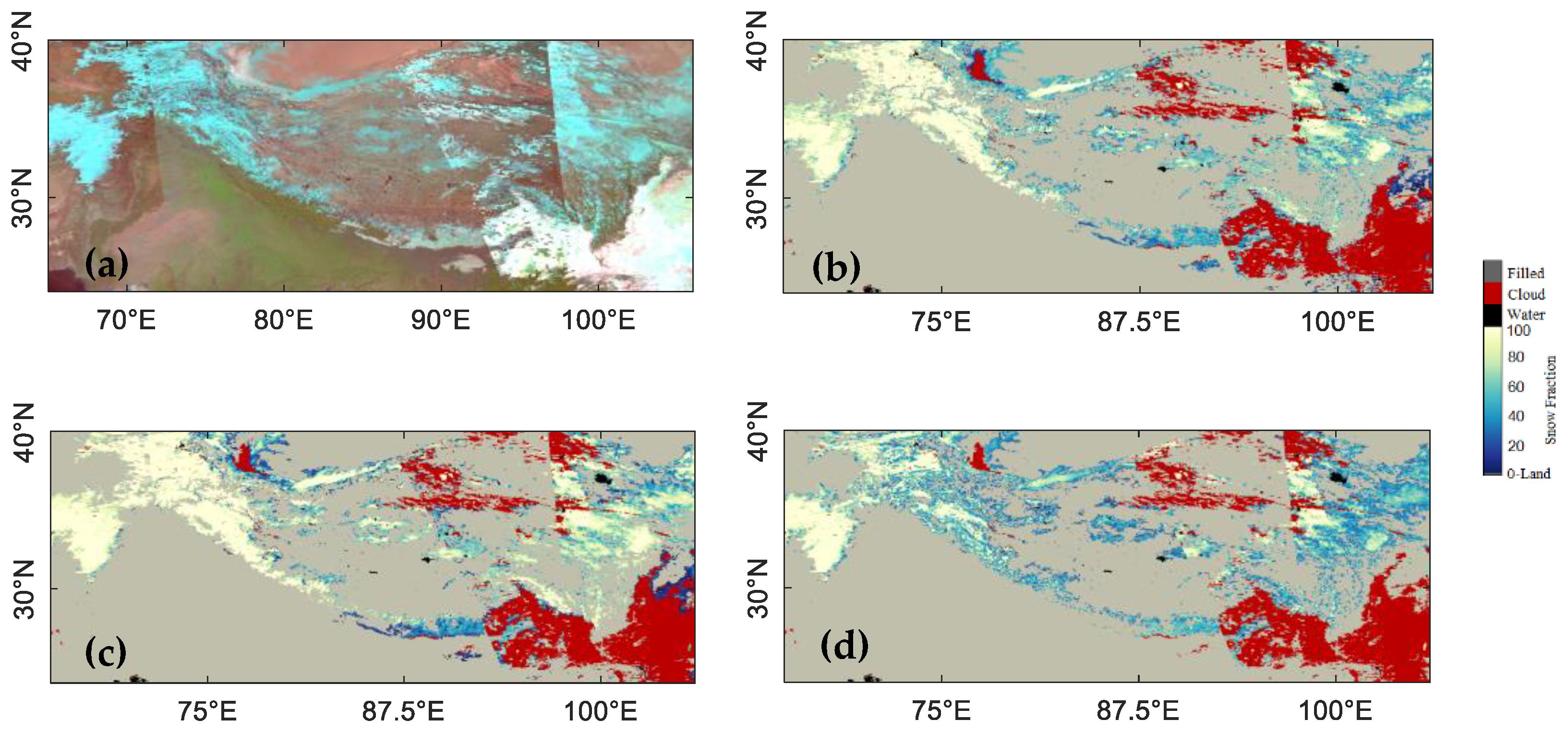
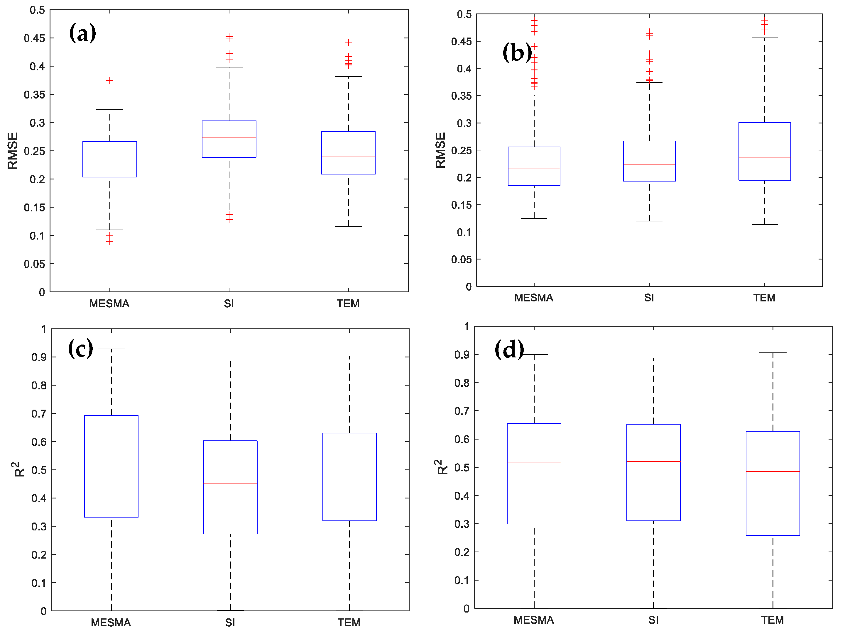
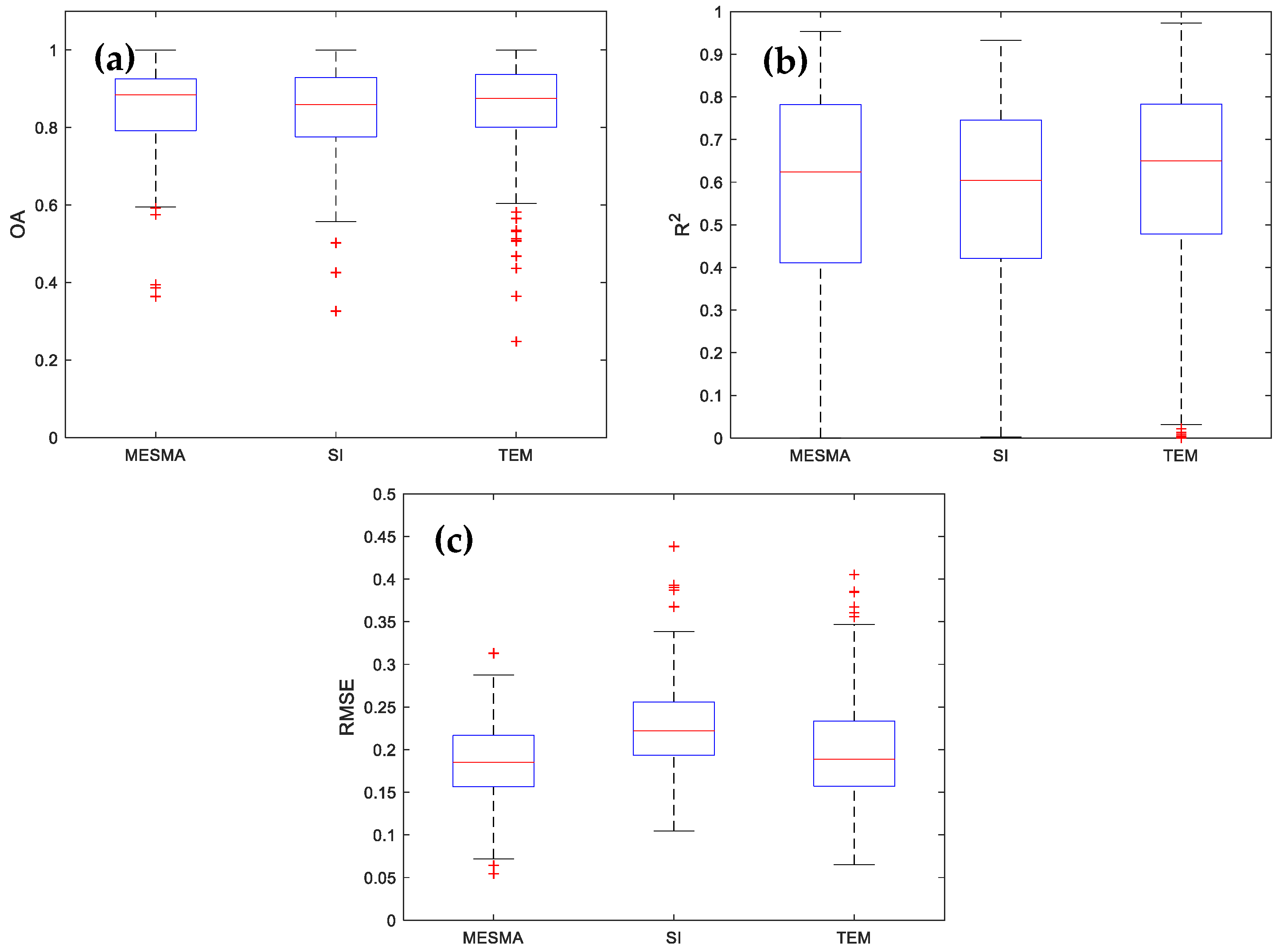
4.1. Results and Evaluation in High Mountain Asia

As clouds identified in the QA index of AVHRR/2 5 km data would be overestimated [34], the MESMA and TEM algorithms could not select effective snow endmembers. Therefore, Hao’s [33] cloud identification algorithm and relevant thresholds were selected for cloud identification. In addition, there is no corresponding cloud identification product for AVHHRR/2 1 km data, so the cloud identification algorithm and relevant thresholds of Zhu [34] were selected for cloud identification. To better reflect the spatial distribution of the three fractional-snow-cover retrieval algorithm results at different scales, one AVHRR/2 scene with a large snow-cover area and less cloud cover was selected as an example. The results are shown in Figure 3 and Figure 4 below.

Figure 3a shows the false colour image synthesized from AVHRR/2 1 km data in bands 1, 2, and 3. The spatially uniform and bright white areas are water clouds, the spatially uneven and turquoise areas are snow or ice clouds, the green areas are vegetation-covered areas, and the grey or brown areas are bare ground areas. The red areas in Figure 3b–d are the areas identified as clouds. By comparing these figures with Figure 3a, we can see that the cloud identification algorithm can effectively identify water clouds and some ice clouds. By further analysing the fractional-snow-cover retrieval results in Figure 3b–d, we find that the MESMA algorithm retrieval result in Figure 3b contains more spatial details than the SI algorithm retrieval result in Figure 3c. Although the retrieval result of the TEM algorithm represented in Figure 3d contains more spatial details than the retrieval result of the MESMA algorithm, the TEM algorithm is affected by satellite orbital splicing, resulting in a certain degree of underestimation in some areas.

Figure 4a shows the false colour image synthesized from AVHRR/2 5 km data in bands 1, 2, and 3. By comparing Figure 3a and Figure 4a, we find that there are more spliced tracks, which also lead to poorer cloud discrimination results in Figure 4b–d. In addition, by further considering Figure 4b–d, the same conclusion as Figure 3b–d is found, i.e., the retrieval result of the MESMA algorithm is better.

Due to the limited observation width of AVHRR/2, at least two tracks of images are needed to cover the entire High Mountain Asia region. However, due to the different transit times of the images from different tracks, there are obvious stitching seams and different brightness values between the left and right sides of the images after stitching, although the radiation is normalized. This also leads to a significant difference in the retrieval results between the left and right sides of the stitching gap for the TEM algorithm, which relies on single-band reflectivity, as shown in Figure 3d and Figure 4d.

Figure 5 shows the comparison of the accuracy evaluation (OA, RMSE, R²) results for the three AVHRR/2 fractional-snow-cover retrieval algorithms at the 1 km and 5 km scales. As seen from Figure 5a,b, the MESMA algorithm has the best median RMSE at both the 1 km and 5 km scales, reaching 0.24 at 1 km and 0.22 at 5 km. Additionally, there are fewer outliers and generally lower values at the 1 km scale. The RMSE at the 5 km scale is better than that at the 1 km scale, which is due to the reduction of errors in coarse resolution caused by geo-positioning bias. According to the comparison results for the R² indices in Figure 5c,d, the MESMA algorithm is the best at both observation scales, and this algorithm is significantly superior to the other two algorithms at the 1 km scale. A similar conclusion can be drawn by comparing the OA metrics in Figure 5e,f. The MESMA algorithm outperforms the other two algorithms and can achieve a value of 0.85 at the 1 km scale.

In addition, the accuracy evaluation results shown in Figure 5 indicate that each accuracy index is poor for the snow index (SI) method. It is difficult to extend the empirical NDSI and FSC relations established with a small number of samples over a certain period of time to a large-scale study of a long time series; doing so would also lead to poor accuracy of the fractional-snow-cover retrieval results due to the use of only one dataset.

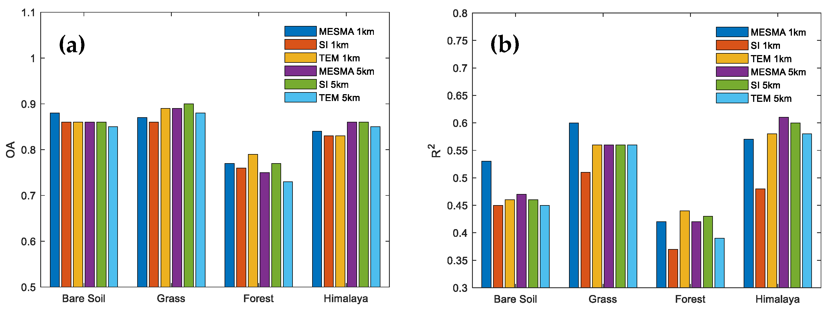
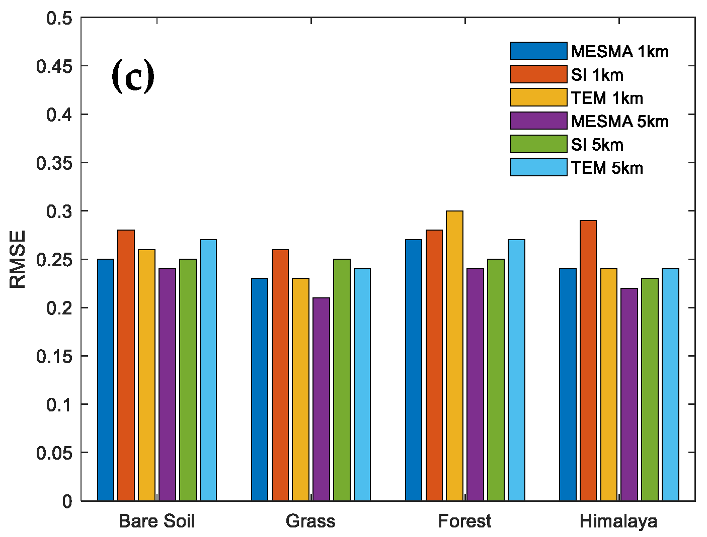
4.2. Evaluation for Different Surface Types

Snow cover impacted by different surface types presents different characteristics; for example, snow cover under forest cover decreases in reflectance due to the shading in forests, which leads to underestimation of snow cover in the region when this is not considered. To quantitatively analyse the accuracy of the three AVHRR/2 fractional-snow-cover retrieval algorithms under different ground cover types, the Landsat-5 validation data were analysed and compared separately according to four typical land types of the High Mountain Asia region: bare land, grassland, forest, and the Himalayan region. The 313 Landsat-5 images used for validation were further classified by surface type into 85 scenes of bare land, 98 scenes of grassland, 83 scenes of forest, and 47 scenes of the Himalayas. The accuracy evaluation was performed under these four surface types, and the related results are shown in Figure 6 below.

The individual accuracy metrics of the three AVHRR/2 fractional-snow-cover retrieval algorithms in Figure 6 demonstrate that, overall, the MESMA algorithm has considerable advantages, and the SI algorithm has the worst results. By further comparing the performance of the three AVHRR/2 fractional-snow-cover retrieval algorithms at the 1 km and 5 km scales, it can be seen that the accuracy metrics of the three AVHRR/2 fractional-snow-cover retrieval algorithms increase at the 5 km scale, especially for the SI algorithm, due to the coarser observation scale and the applicability of the previously fitted empirical relationships. In terms of individual metrics, it can be seen that the accuracy evaluation metrics R² for the three AVHRR/2 fractional-snow-cover retrieval algorithms at the 1 km scale are significantly better than those at the 5 km scale, because the 1 km scale allows more spatial detail to be observed and therefore correlates better with the Landsat-5 results. It can also be seen that each accuracy index of the three AVHRR/2 fractional-snow-cover retrieval algorithms decreases more severely in the forest cover area, which confirms the correctness of the previous analysis.

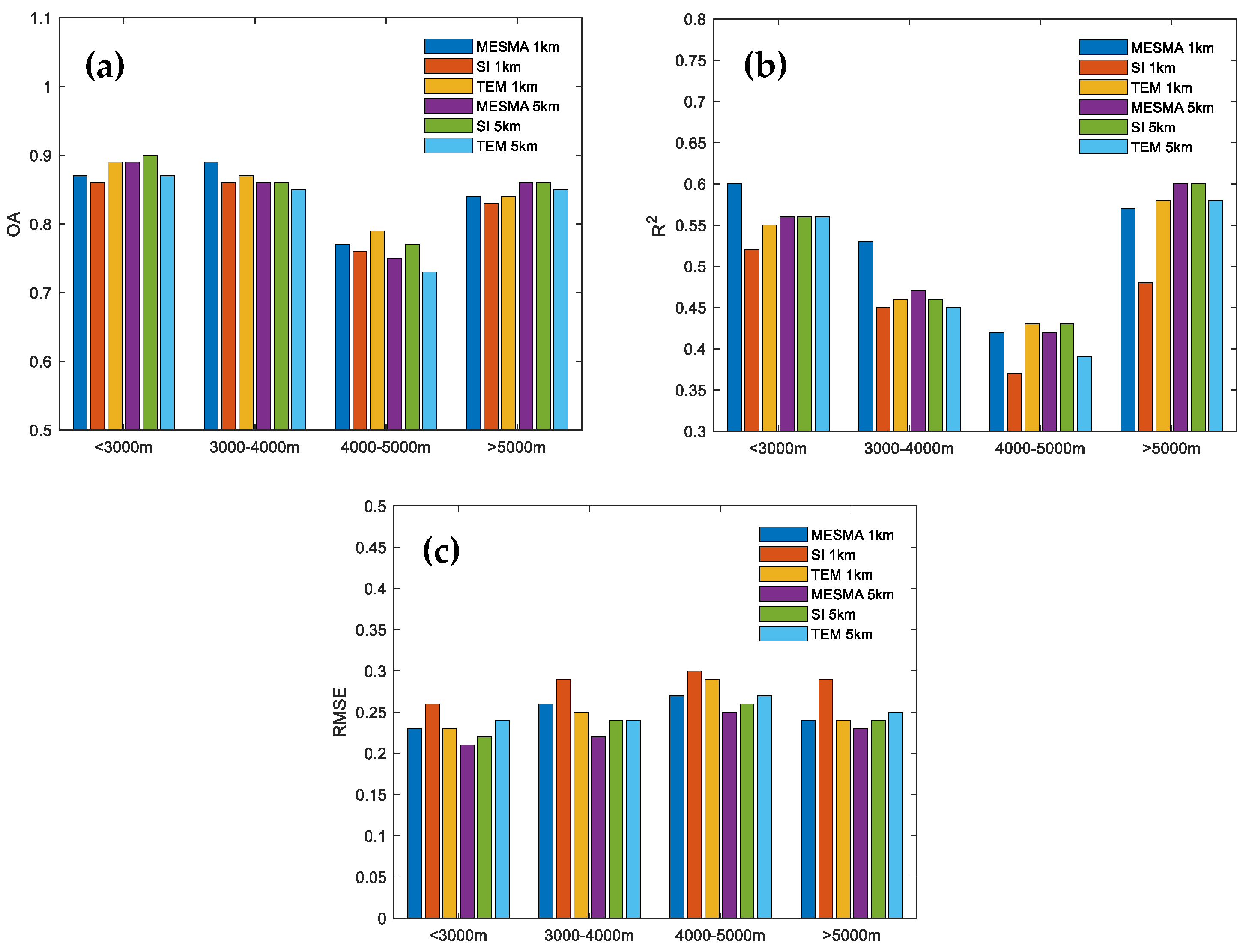
4.3. Evaluation at Different Altitudes

The accuracy of fractional-snow-cover retrieval algorithms is related not only to the surface type but also to the elevation, which has a significant effect on the accuracy. The snow recognition accuracy decreases to a certain extent as the elevation increases [36]. In this study, the 313 scenes used to verify Landsat-5 images were divided into four categories according to altitude: 39 scenes from less than 3000 m, 25 scenes from 3000–4000 m, 108 scenes from 4000–5000 m, and 141 scenes from more than 5000 m. As mentioned previously, when selecting verification images, the set rule is that the proportion of snow-cover area in the whole image should be more than 30%, and verification data are concentrated over three winters. In addition, the average altitude of High Mountain Asia is above 4000 m, so the altitude of the verification images is generally greater than 4000 m. The accuracy evaluation results of the three AVHRR/2 fractional-snow-cover retrieval algorithms at different altitudes are shown in Figure 7 below.

By analysing the accuracy indices of the three AVHRR/2 fractional-snow-cover retrieval algorithms at different altitudes and at different scales in Figure 7, we find that the MESMA algorithm is better than the other two algorithms overall, and both OA and RMSE are higher in the range of less than 4000 m. By comparing the accuracy of each algorithm at different scales, it can be seen that the two accuracy indices OA and RMSE have a certain degree of improvement for each algorithm at the 5 km scale, while R² shows the opposite trend. This is consistent with the reason for the opposite trend of R² for different surface types. From Figure 7a,b, it can be seen that OA and R² show a trend of decreasing and then increasing with increasing altitude, which is consistent with existing AVHRR fractional-snow-cover studies [36]. This phenomenon occurs due to the unique geographical environment of High Mountain Asia and the date for selecting the validation images. Due to the high altitude of the High Mountain Asia region, most of the areas above 5000 m are covered with grass, which leads to severe snow fragmentation, though snow fragmentation is obviously reduced with increasing altitude. Meanwhile, the selected verification images are all from winter, when the proportion of snow-cover area is larger, so the snow in these areas is concentrated, and the verification accuracy is higher.

5. Discussion

The 5 km AVHRR/2 data were resampled from the 1 km data. From the accuracy evaluation results of each algorithm in Figure 5, it can be seen that the three AVHRR/2 fractional-snow-cover retrieval algorithms improved for each accuracy evaluation index at the 5 km scale. However, comparing Figure 3a and Figure 4a, we find that the quality of AVHRR/2 observation data at the 1 km scale is better than that at the 5 km scale. To explore the influence of the observation scale on the fractional-snow-cover retrieval algorithms more reasonably, this study aggregates the snow cover results at the 1 km scale directly to 5 km and then uses validation data from 313 Landsat-5/TM scenes for accuracy evaluation. This study not only quantitatively evaluates the effect of the observation scale on fractional-snow-cover retrieval results but also reflects to a certain extent whether the “upscaling followed by retrieval” method or the “retrieval followed by upscaling” method is better.

Figure 8 shows the accuracy evaluation results for the aggregation of fractional-snow-cover retrieval results from the 1 km scale observation data to the 5 km scale. From Figure 8a, we can see that the MESMA algorithm has the smallest RMSE, reaching 0.18, while the number of outliers is smaller, and the values are lower. From Figure 8b, it can be seen that the R² values of the MESMA algorithm and TEM algorithm are better than that of the SI algorithm. The OA comparison results of the three algorithms are shown in Figure 8c, where it can be seen that the MESMA algorithm achieves the best OA of 0.89. The comprehensive comparison and analysis of Figure 8 shows that the MESMA algorithm is better than the other two AVHRR/2 fractional-snow-cover retrieval algorithms on the whole. This conclusion is consistent with the above findings at the 1 km scale and the 5 km scale.

Comparing Figure 8 and Figure 5a,c,e, it can be seen that the MESMA algorithm always maintains good accuracy. The RMSE improves from 0.24 to 0.18, and the OA improves from 0.82 to 0.89; this improvement is due to the mitigation of snow fragmentation as the scale increases and the fewer errors caused by geolocation. Figure 8 and Figure 5b,d,f show the accuracy evaluation results at the same 5 km scale. Since more spatial details are observed at the 1 km scale, the accuracy is better even when the fractional-snow-cover retrieval results are aggregated to the 5 km scale than the results of fractional-snow-cover retrieval after aggregation to the 5 km scale first. It can also be seen that there are fewer outliers for each accuracy evaluation index from the 1 km aggregation to the 5 km scale, which also highlights the importance of high-resolution observations. The above results also answer the question of whether the “upscaling followed by retrieval” approach is better than the “retrieval followed by upscaling” approach, because the high-spatial-resolution observations can capture more spatial details, and retrieval of the snow cover first can better reflect these spatial details. If scaling is performed first, these spatial details will be lost, and the estimation of the thin and fragmented snow for High Mountain Asia will result in substantial errors.

6. Conclusions

AVHRR has accumulated valuable data for up to 40 years, making it an important tool for long time series and large-scale snow monitoring. Since the early AVHRR/2 sensors have only two reflectivity bands, it is difficult to carry out snow monitoring based on these two bands, resulting in limited accuracy of the existing AVHRR/2 snow classification and fractional-snow-cover retrieval algorithms. In this study, the reflectance in the 3.75 µm mid-infrared band was simulated using a radiative transfer model, which is equivalent to adding an observation to the AVHRR/2 sensor. Based on the reflectance information in three bands, in this study, three fractional-snow-cover retrieval algorithms for the AVHRR/2 sensor were developed. After the validation of high-spatial-resolution Landsat-5/TM images, it was found that the MESMA algorithm outperformed the SI algorithm and the TEM algorithm overall. This is because the MESMA algorithm combines the observed information from the three bands, starting from the image where the snow retrieval is performed, and therefore the results obtained are more reflective of the snow information in the image. In this study, the effect of surface type on the snow retrieval algorithm was also investigated. The three AVHRR/2 fractional-snow-cover retrieval algorithms had good accuracy for bare ground, grassland, and Himalayan areas but were slightly less accurate in forested areas, due to the shading of snow by the forest canopy. A follow-up study will be conducted for forested areas to improve the overall accuracy of the MESMA algorithm. The average altitude of High Mountain Asia is over 4000 m, and the terrain heterogeneity is strong, resulting in thin and broken snow in this region. Classifying the altitude according to the gradient and evaluating the accuracy according to the classification results demonstrated, based on the results, that the accuracy evaluation of the three fractional-snow-cover retrieval algorithms first decreased and then increased with increasing altitude, which is quite consistent with the existing research. Through further analysis, it was found that the poor accuracy in the range of 4000–5000 m was due to the severe snow fragmentation in this area; the early AVHR/2 sensor could not effectively capture this snow feature due to its weak performance. By studying the influence of scale effects on fractional-snow-cover retrieval algorithms, it was found that high-spatial-resolution observations are important for snow monitoring, and it can also be concluded that when performing snow-cover retrieval at different scales, the best accuracy is achieved by first performing snow retrieval and then scale conversion. The above research provides a good basis for the study of long-term and large-scale snow monitoring in the High Mountain Asia region.

References

1. Wulf, H.; Bookhagen, B.; Scherler, D. Differentiating between rain, snow, and glacier contributions to river discharge in the western Himalaya using remote-sensing data and distributed hydrological modeling. Adv. Water Resour. 2016, 88, 152–169. [Google Scholar] [CrossRef] [Green Version]
2. Huang, X.; Deng, J.; Wang, W.; Feng, Q.; Liang, T.G. Impact of climate and elevation on snow cover using integrated remote sensing snow products in Tibetan Plateau. Remote Sens. Environ. 2017, 190, 274–288. [Google Scholar] [CrossRef]
3. Tang, Z.; Ma, J.; Peng, H.; Wang, S.; Wei, J. Spatiotemporal changes of vegetation and their responses to temperature and precipitation in upper Shiyang river basin. Adv. Space Res. 2017, 60, 969–979. [Google Scholar] [CrossRef]
4. Ling, F.; Zhang, T. A numerical model for surface energy balance and thermal regime of the active layer and permafrost containing unfrozen water. Cold Reg. Sci. Technol. 2004, 38, 1–15. [Google Scholar] [CrossRef]
5. Dedieu, J.P.; Lessard-Fontaine, A.; Ravazzani, G.; Cremonese, E.; Shalpykova, G.; Beniston, M. Shifting mountain snow patterns in a changing climate from remote sensing retrieval. Sci. Total Environ. 2014, 493, 1267–1279. [Google Scholar] [CrossRef] [PubMed] [Green Version]
6. Barnett, T.P.; Adam, J.C.; Lettenmaier, D.P. Potential impacts of a warming climate on water availability in snow-dominated regions. Nature 2005, 438, 303–309. [Google Scholar] [CrossRef]
7. Xu, Y.; Jones, A.; Rhoades, A. A quantitative method to decompose SWE differences between regional climate models and reanalysis datasets. Sci. Rep. 2019, 9, 16520. [Google Scholar] [CrossRef] [Green Version]
8. Tang, Z.; Wang, J.; Li, H.; Liang, J.; Wang, X.; Li, H.; Jiang, Z. Extraction and assessment of snowline altitude over the Tibetan plateau using MODIS fractional snow cover data (2001 to 2013). J. Appl. Remote Sens. 2014, 8, 084689. [Google Scholar] [CrossRef]
9. Tang, Z.; Wang, X.; Wang, J.; Wang, X.; Li, H.; Jiang, Z. Spatiotemporal variation of snow cover in Tianshan Mountains, Central Asia, based on cloud-free MODIS fractional snow cover product, 2001–2015. Remote Sens. 2017, 9, 1045. [Google Scholar] [CrossRef] [Green Version]
10. Dozier, J. Spectral Signature of Alpine Snow Cover from the Landsat Thematic Mapper. Remote Sens. Environ. 1989, 28, 9–22. [Google Scholar] [CrossRef]
11. Tang, Z.; Wang, X.; Deng, G.; Wang, X.; Jiang, Z.; Sang, G. Spatiotemporal variation of snowline altitude at the end of melting season across High Mountain Asia, using MODIS snow cover product. Adv. Space Res. 2020, 66, 2629–2645. [Google Scholar] [CrossRef]
12. Deng, G.; Tang, Z.; Hu, G.; Wang, J.; Sang, G.; Li, J. Spatiotemporal dynamics of snowline altitude and their responses to climate change in the Tienshan Mountains, Central Asia, During 2001–2019. Sustainability 2021, 13, 3992. [Google Scholar] [CrossRef]
13. Salomonson, V.V.; Appel, I. Estimating fractional snow cover from MODIS using the normalized difference snow index. Remote Sens. Environ. 2004, 89, 351–360. [Google Scholar] [CrossRef]
14. Salomonson, V.V.; Appel, I. Development of the Aqua MODIS NDSI fractional snow cover algorithm and validation results. IEEE Trans. Geosci. Remote Sens. 2006, 44, 1747–1756. [Google Scholar] [CrossRef]
15. Slater, M.T.; Sloggett, D.R.; Rees, W.G.; Steel, A. Potential operational multi-satellite sensor mapping of snow cover in maritime sub-polar regions. Int. J. Remote Sens. 1999, 20, 3019–3030. [Google Scholar] [CrossRef]
16. Metsämäki, S.; Pulliainen, J.; Salminen, M.; Luojus, K.; Wiesmann, A.; Solberg, R.; Böttcher, K.; Hiltunen, M.; Ripper, E. Introduction to GlobSnow Snow Extent products with considerations for accuracy assessment. Remote Sens. Environ. 2015, 156, 96–108. [Google Scholar] [CrossRef]
17. Metsamaki, S.J.; Anttila, S.T.; Markus, H.J.; Vepsalainen, J.M. A feasible method for fractional snow cover mapping in boreal zone based on a reflectance model. Remote Sens. Environ. 2005, 95, 77–95. [Google Scholar] [CrossRef]
18. Painter, T.H.; Dozier, J.; Roberts, D.A.; Davis, R.E.; Green, R.O. Retrieval of subpixel snow-covered area and grain size from imaging spectrometer data. Remote Sens. Environ. 2003, 85, 64–77. [Google Scholar] [CrossRef] [Green Version]
19. Painter, T.H.; Rittger, K.; McKenzie, C.; Slaughter, P.; Davis, R.E.; Dozier, J. Retrieval of subpixel snow covered area, grain size, and albedo from MODIS. Remote Sens. Environ. 2009, 113, 868–879. [Google Scholar] [CrossRef] [Green Version]
20. Rittger, K.; Painter, T.H.; Dozier, J. Assessment of methods for mapping snow cover from MODIS. Adv. Water Resour. 2013, 51, 367–380. [Google Scholar] [CrossRef]
21. Sirguey, P.; Mathieu, R.; Arnaud, Y. Subpixel monitoring of the seasonal snow cover with MODIS at 250 m spatial resolution in the Southern Alps of New Zealand: Methodology and accuracy assessment. Remote Sens. Environ. 2009, 113, 160–181. [Google Scholar] [CrossRef]
22. Moosavi, V.; Malekinezhad, H.; Shirmohammadi, B. Fractional snow cover mapping from MODIS data using wavelet-artificial intelligence hybrid models. J. Hydrol. 2014, 511, 160–170. [Google Scholar] [CrossRef]
23. Czyzowska-Wisniewski, E.H.; van Leeuwen, W.J.D.; Hirschboeck, K.K.; Marsh, S.E.; Wisniewski, W.T. Fractional snow cover estimation in complex alpine-forested environments using an artificial neural network. Remote Sens. Environ. 2015, 156, 403–417. [Google Scholar] [CrossRef]
24. Kuter, S.; Akyurek, Z.; Weber, G.W. Retrieval of fractional snow covered area from MODIS data by multivariate adaptive regression splines. Remote Sens. Environ. 2018, 205, 236–252. [Google Scholar] [CrossRef]
25. Hou, J.; Huang, C.; Chen, W.; Zhang, Y. Improving Snow Estimates Through Assimilation of MODIS Fractional Snow Cover Data Using Machine Learning Algorithms and the Common Land Model. Water Resour. Res. 2021, 57, e2020WR029010. [Google Scholar] [CrossRef]
26. Kuter, S. Completing the machine learning saga in fractional snow cover estimation from MODIS Terra reflectance data: Random forests versus support vector regression. Remote Sens. Environ. 2021, 255, 112294. [Google Scholar] [CrossRef]
27. Rittger, K.; Krock, M.; Kleiber, W.; Bair, E.H.; Brodzik, M.J.; Stephenson, T.R.; Rajagopalan, B.; Bormann, K.J.; Painter, T.H. Multi-sensor fusion using random forests for daily fractional snow cover at 30 m. Remote Sens. Environ. 2021, 264, 112608. [Google Scholar] [CrossRef]
28. Hall, D.K.; Riggs, G.A.; Salomonson, V.V. Development of Methods for Mapping Global Snow Cover Using Moderate Resolution Imaging Spectroradiometer Data. Remote Sens. Environ. 1995, 54, 127–140. [Google Scholar] [CrossRef]
29. Riggs, G.A.; Hall, D.K.; Román, M.O. MODIS Snow Products Collection 6 User Guide. 2016. Available online: https://nsidc.org/sites/nsidc.org/files/files/MODIS-snow-user-guide-C6.pdf (accessed on 15 March 2021).
30. Wang, G.; Jiang, L.; Shi, J.; Su, X. A Universal Ratio Snow Index for Fractional Snow Cover Estimation. IEEE Geosci. Remote Sens. Lett. 2021, 18, 721–725. [Google Scholar] [CrossRef]
31. Naegeli, K.N.; Salberg, A.B.; Schwaizer, G.; Wiesmann, A.; Wunderle, S.; Nagler, T. ESA Snow Climate Change Initiative (Snow_cci): Daily global Snow Cover Fraction—Snow on ground (SCFG) from AVHRR (1982–2019), version 1.0. NERCEDS Centre for Environmental Data Analysis [dataset]. 2021. Available online: https://catalogue.ceda.ac.uk/uuid/5484dc1392bc43c1ace73ba38a22ac56 (accessed on 15 December 2021).
32. Hori, M.; Sugiura, K.; Kobayashi, K.; Aoki, T.; Tanikawa, T.; Kuchiki, K.; Niwano, M.; Enomoto, H. A 38-year (1978–2015) Northern Hemisphere daily snow cover extent product derived using consistent objective criteria from satellite-borne optical sensors. Remote Sens. Environ. 2017, 191, 402–418. [Google Scholar] [CrossRef]
33. Hao, X.; Huang, G.; Che, T.; Ji, W.; Sun, X.; Zhao, Q.; Zhao, H.; Wang, J.; Li, H.; Yang, Q. The NIEER AVHRR snow cover extent product over China—A long-term daily snow record for regional climate research. Earth Syst. Sci. Data 2021, 13, 4711–4726. [Google Scholar] [CrossRef]
34. Zhu, J.; Shi, J. An Algorithm for Subpixel Snow Mapping: Extraction of a Fractional Snow-Covered Area Based on Ten-Day Composited AVHRR/2 Data of the Qinghai-Tibet Plateau. IEEE Geosci. Remote Sens. Mag. 2018, 6, 86–98. [Google Scholar] [CrossRef]
35. Shi, J. An Automatic Algorithm on Estimating Sub-Pixel Snow Cover from MODIS. Quat. Sci. 2012, 32, 6–15. [Google Scholar]
36. Wu, X.; Naegeli, K.; Premier, V.; Marin, C.; Ma, D.; Wang, J.; Wunderle, S. Evaluation of snow extent time series derived from Advanced Very High Resolution Radiometer global area coverage data (1982–2018) in the Hindu Kush Himalayas. Cryosphere 2021, 15, 4261–4279. [Google Scholar] [CrossRef]
37. Zhang, Y.; Ren, H.; Pan, X. Integration dataset of Tibet Plateau boundary. National Tibetan Plateau Data Center [dataset]. 2021. Available online: http://data.tpdc.ac.cn (accessed on 15 March 2022). [CrossRef]
38. Reuter, H.I.; Nelson, A.; Jarvis, A. An evaluation of void-filling interpolation methods for SRTM data. Int. J. Geogr. Inf. Sci. 2007, 21, 983–1008. [Google Scholar] [CrossRef]
39. Chinese Academy of Sciences Resource and Environmental Science Data Center. Landuse dataset in China (1980–2015) [data set]. National Tibetan Plateau Data Center. 2019. Available online: http://www.resdc.cn/ (accessed on 15 October 2021).
40. Salisbury, J.W. Johns Hopkins University Spectral Library and ASTER Spectral Library [dataset]. 2002. Available online: http://speclib.jpl.nasa.gov (accessed on 15 October 2021).
41. Roger, J.C.; Vermote, E.F. A method to retrieve the reflectivity signature at 3.75 μm from AVHRR data. Remote Sens. Environ. 1998, 64, 103–114. [Google Scholar] [CrossRef]
42. Kaufman, Y.J.; Kleidman, R.G.; Hall, D.K.; Martins, J.V.; Barton, J.S. Remote sensing of subpixel snow cover using 0.66 and 2.1 μm channels. Geophys. Res. Lett. 2002, 29, 28-1–28-4. [Google Scholar] [CrossRef]
43. Wang, G.; Jiang, L.; Wu, S.; Shi, J.; Hao, S.; Liu, X. Fractional Snow Cover Mapping from FY-2 VISSR Imagery of China. Remote Sens. 2017, 9, 983. [Google Scholar] [CrossRef] [Green Version]
44. Yang, J.; Jiang, L.; Shi, J.; Wu, S.; Sun, R.; Yang, H. Monitoring snow cover using Chinese meteorological satellite data over China. Remote Sens. Environ. 2014, 143, 192–203. [Google Scholar] [CrossRef]
45. Adams, J.B.; Smith, M.O.; Johnson, P.E. Spectral Mixture Modeling—A New Analysis of Rock and Soil Types at the Viking Lander-1 Site. J. Geophys. Res.-Solid Earth Planets 1986, 91, 8098–8112. [Google Scholar] [CrossRef]
46. Bateson, A.; Curtiss, B. A method for manual endmember selection and spectral unmixing. Remote Sens. Environ. 1996, 55, 229–243. [Google Scholar] [CrossRef]
47. Heinz, D.C.; Chang, C.I. Fully constrained least squares linear spectral mixture analysis method for material quantification in hyperspectral imagery. IEEE Trans. Geosci. Remote Sens. 2001, 39, 529–545. [Google Scholar] [CrossRef] [Green Version]
Figure 1. The land cover type map of High Mountain Asia. The spatial extent of Landsat–5 Thematic Mapper (TM).
Remotesensing 14 03303 g001
Figure 2. The 3.75 μm band reflectivity scatter density plot for the results of this study compared to the official product results.
Remotesensing 14 03303 g002
Figure 3. Comparison of the results from the three fractional-snow-cover algorithms on the 1 km scale for High Mountain Asia (25 January 1993): (a) the false colour image of AVHRR/2 bands 1, 2, and 3; (b) FSC from AVHRR/2 using the MESMA algorithm; (c) FSC from AVHRR/2 using the SI algorithm; (d) FSC from AVHRR/2 using the TEM algorithm.
Remotesensing 14 03303 g003
Figure 4. Comparison of the results from the three fractional-snow cover algorithms on the 5 km scale for High Mountain Asia (25 January 1993): (a) the false colour image of AVHRR/2 Bands 1, 2, and 3; (b) FSC from AVHRR/2 using the MESMA algorithm; (c) FSC from AVHRR/2 using the SI algorithm; (d) FSC from AVHRR/2 using the TEM algorithm.
Remotesensing 14 03303 g004
Figure 5. Boxplots of accuracy evaluation results for three AVHRR/2 fractional-snow-cover retrieval algorithms at 1 km and 5 km scales, based on 313 Landsat-5/TM scenes: (a) the RMSE of the three AVHRR/2 FSC retrieval algorithms at 1 km scale; (b) the RMSE of the three AVHRR/2 FSC retrieval algorithms at 5 km scale; (c) the R2 of the three AVHRR/2 FSC retrieval algorithms at 1 km scale; (d) the R2 of the three AVHRR/2 FSC retrieval algorithms at 5 km scale; (e) the OA of the three AVHRR/2 FSC retrieval algorithms at 1 km scale; (f) the OA of the three AVHRR/2 FSC retrieval algorithms at 5 km scale.
Remotesensing 14 03303 g005aRemotesensing 14 03303 g005b
Figure 6. Accuracy evaluation results under different surface types for three AVHRR/2 fractional-snow-cover retrieval algorithms at 1 km and 5 km scales based on 313 Landsat-5/TM scenes: (a) the OA of the three AVHRR/2 FSC retrieval algorithms at 1 km and 5 km scales; (b) the R2 of the three AVHRR/2 FSC retrieval algorithms at 1 km and 5 km scales; (c) the OA of the three AVHRR/2 FSC retrieval algorithms at 1 km and 5 km scales.
Remotesensing 14 03303 g006aRemotesensing 14 03303 g006b
Figure 7. Accuracy evaluation results at different altitudes for three AVHRR/2 fractional snow cover retrieval algorithms at 1 km and 5 km scales based on 313 Landsat–5/TM scenes: (a) the OA of the three AVHRR/2 FSC retrieval algorithms at 1 km and 5 km scales; (b) the R2 of the three AVHRR/2 FSC retrieval algorithms at 1 km and 5 km scales; (c) the RMSE of the three AVHRR/2 FSC retrieval algorithms at 1 km and 5 km scales.
Remotesensing 14 03303 g007
Figure 8. Boxplots of accuracy evaluation results for the three AVHRR/2 FSC retrieval algorithms from 1 km aggregation to 5 km scale: (a) the RMSE of the three AVHRR/2 FSC retrieval algorithms at 1 km aggregation to 5 km scale; (b) the R2 of the three AVHRR/2 FSC retrieval algorithms at 1 km aggregation to 5 km scale; (c) the OA of the three AVHRR/2 FSC retrieval algorithms at 1 km aggregation to 5 km scale.
Remotesensing 14 03303 g008