Deep-Learning-Based Multiple Model Tracking Method for Targets with Complex Maneuvering Motion

Abstract

The effective detection of unmanned aerial vehicle (UAV) targets is of great significance to guarantee national military security and social stability. In recent years, with the development of communication and control technology, the movement of UAVs has become increasingly flexible and complex, presenting diverse trajectory forms and different motion models in different phases. The Gaussian mixture probability hypothesis density filter incorporating the linear Gaussian jump Markov system approach (LGJMS-GMPHD) provides an efficient method for tracking multiple maneuvering targets, as applied to the switching of motions between a set of models in a Markovian chain. However, in practice, the motion model parameters of targets are generally unknown and the model switching is uncertain. When the preset filtering model parameters are mismatched, the tracking performance is dramatically degraded. In this paper, within the framework of the LGJMS-GMPHD filter, a deep-learning-based multiple model tracking method is proposed. First, an adaptive turn rate estimation network is designed to solve the filtering model mismatch caused by unknown turn rate parameters in coordinate turn models. Second, a filter state modification network is designed to solve the large tracking errors in the maneuvering phase caused by uncertain motion model switching. Finally, based on simulations of multiple maneuvering targets in cluttered environments and experimental field data verification, it can be concluded that the proposed method has strong adaptability to multiple maneuvering forms and can effectively improve the tracking performance of targets with complex maneuvering motion.

1. Introduction

Unmanned aerial vehicles (UAVs), with their advantages of flexible usage and easy deployment, have been widely used in many fields, including military applications such as battlefield surveillance, air reconnaissance, and tracking, as well as in civilian applications such as disaster monitoring, geophysical exploration, and agricultural plant protection [1]. At the same time, their malicious use also poses a severe threat to aviation security and the maintenance of social stability [2]. Radar has proven to be an essential technical method of UAV detection [3,4]. However, the strong maneuverability of UAVs, including their unknown motion model parameters and uncertain model switching [5], brings about great challenges in the stable tracking of targets.

Random finite set (RFS)-based filters provide a theoretically optimal approach to multi-target tracking and are widely used in many fields [6,7,8]. In the RFS formulation, the collection of target states at any given time is regarded as a set-valued multi-target state, and the collection of measurements is regarded as a set-valued multi-target observation [9,10]. Then, the problem of dynamically estimating multiple targets can be formulated in a Bayesian filtering framework by propagating the posterior distribution of the multi-target state in time. However, multi-target filtering solutions in their standard form are generally implemented by a fixed motion model. Thus, to characterize the a rapidly maneuvering target with multiple models, the jump Markov system (JMS) approach has been incorporated into the existing RFS-based filters. Mahler derived the probability hypothesis density (PHD) filter and cardinalized probability hypothesis density (CPHD) filter approximations of the jump Markov multitarget Bayes filter [11]. On this basis, a closed-form solution to the PHD recursion for the linear Gaussian jump Markov multi-target model was derived, and this is referred as the LGJMS-GMPHD filter [12]. In addition, the JMS approach has also been incorporated into CPHD [13], multi-Bernoulli [14], and labeled multi-Bernoulli filters [7]. However, in the above multiple model filters, the constant velocity (CV) and coordinate turn (CT) models are generally combined as model sets to describe the maneuvering motion. When these are applied to practical UAV tracking scenarios, there are two key problems: (i) the turn rate of the target is generally unknown, resulting in a mismatch between the target’s motion and the CT filtering model; (ii) for complex maneuvering trajectories, the uncertainty of motion model switching leads to the degradation of tracking performance.

There are two common approaches to estimating the turn rate. The first class estimates the turn rate online by using the estimated acceleration magnitude over the estimated speed [15]. However, the estimated acceleration is generally not accurate enough, leading to inaccurate turn rate estimates. For the second class, the turn rate parameter is augmented into the state vector and the turn rate is estimated as part of the state vector recursively, which creates a difficult nonlinear problem [16]. Furthermore, target Doppler measurements usually have higher precision compared with position estimates, and thus they have been incorporated to improve the accuracy of the turn rate estimate. In [17], four possible turn rates were estimated based on the Doppler measurement. Due to the lack of prior information on target motion, the minimum turn rate and its opposite value were chosen to be the possible turn rates, and an interacting multiple model (IMM) algorithm consisting of one CV model and two CT models was adopted, increasing the computational burden.

The uncertainty of motion model switching is also a challenging problem in multiple model (MM) filters. In this case, the filtering state estimate has a delay in its response to target maneuvers, so the tracking precision degrades rapidly in the maneuvering phase. A smoothing process can produce delayed estimates, i.e., obtaining the target state estimates at time $k$ given the measurements up to time $k+d\left(d>0\right)$, which contributes to improving the tracking performance of maneuvering targets and has been incorporated into the MM algorithms [18,19,20]. A sequential Monte Carlo (SMC) implementation for MMPHD smoothing was derived in [21] to improve the capability of PHD-based tracking algorithms. However, the backward smoothing procedure is still model-based and cannot extract temporal correlations, so longer lags do not yield better estimates of the current state. Moreover, closed-form recursion with a smoothing process needs to be derived for different filters respectively and the computation is generally intractable, leading to limitations in its applications. Deep neural networks have strong capability of fitting if there are sufficient training data [22], which is conducive to solving the problems of model mismatch and estimation delays in existing MM filtering algorithms for targets with complex maneuvering motions. In [23], a deep learning maneuvering target tracking algorithm was proposed. However, the input of the network was the filtering states estimated by a single-model unscented Kalman filter. For strong maneuvering trajectories, large tracking errors increase the training burden of the network and reduce the convergence rate of training losses. Additionally, an LSTM-based deep recurrent neural network was presented in [24] to overcome the limits of traditional model-based methods, but only CV and constant acceleration (CA) motions were verified, without considering CT maneuvers. Furthermore, the above methods are not suitable for scenarios with multiple maneuvering targets.

In view of the above problems, within the framework of the LGJMS-GMPHD filter, we propose a deep-learning-based multiple model tracking method for multiple maneuvering targets with complex maneuvering motions. The main contributions of this study are summarized as follows:

• An adaptive turn rate estimation network (ATN) is designed. The feature matrix, including multi-frame and multi-dimensional kinematic states, is constructed and used as the input of the network. The temporal correlation information at each previous time step and the weight of different variables are extracted to improve the estimation accuracy of the turn rate. Then, the parameter is fed back to the CT model to enhance the consistency of the target motion and filtering model.
• A filter state modification network (FMN) is designed to smooth the state estimates of the filter. The relationship information between all time steps of the state vector, including position estimates, is extracted to improve the adaptability of the filter to complex maneuvering motions, thereby reducing the tracking errors caused by uncertain model switching.

The remainder of this paper is structured as follows. Section 2 reviews the PHD recursion for the linear Gaussian jump Markov multi-target model. Section 3 presents the principle of the proposed deep-learning-based multiple model tracking method. Section 4 designs the network parameters and verifies the effectiveness of the method in improving tracking performance. The simulation results and experimental data verification are analyzed in Section 5. The discussion and future work are presented in Section 6, and our conclusions are presented in Section 7.

2. Principle of LGJMS-GMPHD

The PHD filter [25] recursively propagates the first order moment or the intensity function associated with the multi-target posterior density, which has the advantage of low computational complexity and has been widely used. Furthermore, a closed-form solution to the PHD recursion for LGJMS derived in [12] provides an efficient method for tracking multiple maneuvering targets. In this section, a short review of RFS and the PHD recursion for the linear Gaussian jump Markov multi-target model is presented.

2.1. Random Finite Sets in Multi-Target Tracking

(1)

Dynamic model

For a given multi-target state $X_{k-1}$ at time $k-1$, each ${\mathit{x}}_{k-1}\in X_{k-1}$ either continues to exist at time $k$ with probability $p_{S,k}\left({\mathit{x}}_{k-1}\right)$, or dies with probability $1-p_{S,k}\left({\mathit{x}}_{k-1}\right)$. Consequently, at the next time step, the behavior of the given state ${\mathit{x}}_{k-1}\in X_{k-1}$ is modelled as the RFS

$$S_{k|k-1}\left({\mathit{x}}_{k-1}\right)$$

(1)

which can take on either $\left\{{\mathit{x}}_k\right\}$ when the target survives, or $\varnothing$ when the target dies. For the sake of simplicity, spawned targets are not considered here. The multi-target state $X_k$ at time $k$ is given by the union of the surviving targets and the spontaneous births:

$$X_k=\left\{\underset{x_{k-1}\in X_{k-1}}{\cup }{S}_{k|k-1}\left({\mathit{x}}_{k-1}\right)\right\}\cup {\Gamma }_k,$$

(2)

where ${\Gamma }_k$ is the RFS of spontaneous birth at time $k$. Each target state ${\mathit{x}}_k={\left[\begin{array}{cccc}{x}_k& {\stackrel{.}{x}}_k& y_k& {\stackrel{.}{y}}_k\end{array}\right]}^T$ denotes the position and velocity of the $x$-axis and $y$-axis.

For the linear Gaussian multi-target model [12], the multi-target transition density is represented as:

$$f_{k|k-1}\left({\mathit{x}}_k|{\mathit{x}}_{k-1}\right)=\mathcal{N}\left({\mathit{x}}_k;{\mathit{F}}_{k-1}{\mathit{x}}_{k-1},{\mathit{Q}}_{k-1}\right),$$

(3)

where $\mathcal{N}\left(\mathbf{·};\mathit{m},\mathit{P}\right)$ denotes a Gaussian density with mean $\mathit{m}$ and covariance $\mathit{P}$; ${\mathit{F}}_{k-1}$ is the state transition matrix; ${\mathit{Q}}_{k-1}$ is the process noise covariance.

In general, motion along a fixed heading at constant speed can be described by a CV model, and a level turn can be described by a CT model. At a turn rate of $0°s^{-1}$, the CT model reduces to the CV model. Therefore, the transition matrix can be uniformly expressed as:

$$F_{k-1}=\left[\begin{array}{cccc}1& \frac{\sin \omega T}{\omega }& 0& -\frac{1-\cos \omega T}{\omega }\\ 0& \cos \omega T& 0& -\sin \omega T\\ 0& \frac{1-\cos \omega T}{\omega }& 1& \frac{\sin \omega T}{\omega }\\ 0& \sin \omega T& 0& \cos \omega T\end{array}\right],$$

(4)

where $T$ is the sample interval and $\omega$ is the turn rate, which is defined as the rate of change of the (velocity) heading angle in the horizontal plane and estimated as the magnitude of the acceleration divided by the speed of the target [15]. In this paper, we refer to this method as the physical definition method (PDM).

(2)

Measurement model

The RFS measurement model, which accounts for detection uncertainty and clutter, is described as follows. A given target ${\mathit{x}}_k\in X_k$ is either detected with probability $p_{D,k}\left({\mathit{x}}_k\right)$ or missed with probability $1-p_{D,k}\left({\mathit{x}}_k\right)$. At time $k$, each state ${\mathit{x}}_k\in X_k$ generates an RFS

$${\Theta }_k\left({\mathit{x}}_k\right)$$

(5)

that can take on either $\left\{{\mathit{z}}_k\right\}$ when the target is detected, or $\varnothing$ when the target is not detected. Given a multi-target state $X_k$ at time $k$, the multi-target measurement $Z_k$ received at the sensor is formed by the union of target generated measurements and clutter, i.e.,

$$Z_k=K_k\cup \left[{\displaystyle \underset{\mathit{x}\in X_k}{\cup }{\Theta }_k\left(\mathit{x}\right)}\right].$$

(6)

For the linear Gaussian multi-target model, the multitarget likelihood is represented as:

$$g_k\left({\mathit{z}}_k|{\mathit{x}}_k\right)=\mathcal{N}\left({\mathit{z}}_k;{\mathit{H}}_k{\mathit{x}}_k,{\mathit{R}}_k\right),$$

(7)

where ${\mathit{H}}_k$ is the observation matrix and ${\mathit{R}}_k$ is the measurement noise covariance.

Target Doppler measurements may provide additional information about the target’s kinematic state and therefore can be incorporated into the tracker to enhance the tracking performance [26]. After the Doppler is introduced, each measurement at time $k$ is denoted as ${\mathit{z}}_k=\left[\begin{array}{ccc}{x}_k^m& y_k^m& {\stackrel{.}{r}}_k^m\end{array}\right]$, where $x_k^m$ and $y_k^m$ are the positions of $x$-axis and $y$-axis, and ${\stackrel{.}{r}}_k^m$ is the Doppler. The modified measurement equation is expressed as follows:

$${\mathit{z}}_k=h_k\left({\mathit{x}}_k\right)+{\mathit{n}}_k=\left[\begin{array}{c}{x}_k^m\\ y_k^m\\ {\stackrel{.}{r}}_k^m\end{array}\right]=\left[\begin{array}{c}{x}_k\\ y_k\\ {\stackrel{.}{r}}_k\end{array}\right]+\left[\begin{array}{c}{n}_k^x\\ n_k^y\\ n_k^d\end{array}\right],$$

(8)

$${\stackrel{.}{r}}_k=h_{d,k}\left(x_k\right)=\frac{x_k{\stackrel{.}{x}}_k+y_k{\stackrel{.}{y}}_k}{\sqrt{x_k^2+y_k^2}},$$

(9)

where ${\mathit{n}}_k$ is Gaussian measurement noise with mean zero and covariance $R_k=diag\left({\sigma }_x^2,{\sigma }_y^2,{\sigma }_d^2\right)$, ${\sigma }_x^2$ and ${\sigma }_y^2$ are the position noise variance, and ${\sigma }_d^2$ is the Doppler noise variance. Obviously, the Doppler measurement function $h_{d,k}(·)$ is nonlinear.

In this paper, to simplify the operation, we take the Taylor series expansion of (9) at $x_k$ to linearize the measurement equation. Then, the observation matrix is modified as:

$$H_k=\left[\begin{array}{l}\hspace{1em}1\hspace{1em} 0\hspace{1em} 0\hspace{1em} 0\\ \hspace{1em}0\hspace{1em} 1\hspace{1em} 0\hspace{1em} 0\\ \frac{\partial {\stackrel{.}{r}}_k}{\partial x_k} \frac{\partial {\stackrel{.}{r}}_k}{\partial y_k} \frac{\partial {\stackrel{.}{r}}_k}{\partial {\stackrel{.}{x}}_k} \frac{\partial {\stackrel{.}{r}}_k}{\partial {\stackrel{.}{y}}_k}\end{array}\right],$$

(10)

where

$$\begin{array}{l}\frac{\partial {\stackrel{.}{r}}_k}{\partial x_k}=\left({\stackrel{.}{x}}_k{y}_k^2-x_k{y}_k·{\stackrel{.}{y}}_k\right)/{\left(x_k^2+y_k^2\right)}^{3/2}\\ \frac{\partial {\stackrel{.}{r}}_k}{\partial y_k}=\left({\stackrel{.}{y}}_k{x}_k^2-x_k{y}_k·{\stackrel{.}{x}}_k\right)/{\left(x_k^2+y_k^2\right)}^{3/2}\\ \frac{\partial {\stackrel{.}{r}}_k}{\partial {\stackrel{.}{x}}_k}=x_k/{\left(x_k^2+y_k^2\right)}^{1/2}\\ \frac{\partial {\stackrel{.}{r}}_k}{\partial {\stackrel{.}{y}}_k}=y_k/{\left(x_k^2+y_k^2\right)}^{1/2}\end{array}$$

(11)

2.2. PHD Recursion for LGJMS Multi-Target Model

JMS provides a natural means to model a maneuvering target for which the behavior cannot always be characterized by a single model. It is described by a set of parameterized state space models, the underlying parameters of which evolve with time according to a finite state Markov chain [12]. Suppose that ${\mu }_k\in \mathcal{M}$ is the label of the model in effect at time $k$, where $\mathcal{M}$ denotes the (discrete) set of all model labels. The models follow a discrete Markov chain with transition probability $t_{k|k-1}\left({\mu }_k|{\mu }_{k-1}\right)$. The state vector is augmented as $x_k={\left[{\xi }_k^T,{\mu }_k\right]}^T\in \chi ={ℝ}^n\times \mathcal{M}$ and the transition is governed by

$$f_{k|k-1}\left({\mathit{x}}_k|{\mathit{x}}_{k-1}\right)={\tilde{f}}_{k|k-1}\left({\mathit{\xi }}_k|{\mathit{\xi }}_{k-1},{\mu }_k\right)t_{k|k-1}\left({\mu }_k|{\mu }_{k-1}\right).$$

(12)

The corresponding measurement likelihood is

$$g_k\left({\mathit{z}}_k|{\mathit{x}}_k\right)=g_k\left({\mathit{z}}_k|{\mathit{\xi }}_k,{\mu }_k\right).$$

(13)

For a JMS with linear Gaussian models, the state transition density and measurement likelihood conditioned on mode ${\mu }_k$ are given by

$${\tilde{f}}_{k|k-1}\left({\xi }_k|{\xi }_{k-1},{\mu }_k\right)=\mathcal{N}\left({\xi }_k;F_{k-1}\left({\mu }_k\right){\xi }_{k-1},Q_{k-1}\left({\mu }_k\right)\right),$$

(14)

$$g_k\left({\mathit{z}}_k|{\xi }_k,{\mu }_k\right)=\mathcal{N}\left({\mathit{z}}_k;{\mathit{H}}_k\left({\mu }_k\right){\xi }_k,R_k\left({\mu }_k\right)\right),$$

(15)

where $F_{k-1}\left({\mu }_k\right)$ and $H_k\left({\mu }_k\right)$ denote the transition and the observation matrices of model ${\mu }_k$, and $Q_{k-1}\left({\mu }_k\right)$ and $R_k\left({\mu }_k\right)$ denote covariance matrices of the process noise and measurement noise.

The purpose of maneuvering target tracking is to estimate the augmented state $x_k$ at time $k$ from the sequence of measurement sets ${\mathit{z}}_{1:k}=\left({\mathit{z}}_1,\dots ,{\mathit{z}}_k\right)$. The closed-form PHD recursion for the LGJMS multi-target model [12] is presented as follows:

• Prediction step

For an LGJMS multi-target model, if the posterior intensity $v_{k-1}$ at time $k-1$ has the form

$$v_{k-1}\left({\mathit{\xi }}_{k-1},{\mu }_{k-1}\right)={\displaystyle \sum _{i=1}^{J_{k-1}\left({\mu }_{k-1}\right)}{w}_{k-1}^{\left(i\right)}\left({\mu }_{k-1}\right)\mathcal{N}\left({\mathit{\xi }}_{k-1};{\mathit{m}}_{k-1}^{\left(i\right)}\left({\mu }_{k-1}\right),{\mathit{P}}_{k-1}^{\left(i\right)}\left({\mu }_{k-1}\right)\right)},$$

(16)

then the predicted intensity $v_{k|k-1}$ is given by

$$v_{k|k-1}\left({\xi }_k,{\mu }_k\right)=v_{S,k|k-1}\left({\xi }_k,{\mu }_k\right)+v_{\gamma ,k}\left({\xi }_k,{\mu }_k\right),$$

(17)

where $v_{\gamma ,k}\left({\xi }_k,{\mu }_k\right)$ is the intensity of birth targets, and the intensity of survival targets is represented as:

$$v_{S,k|k-1}\left({\mathit{\xi }}_k,{\mu }_k\right)={\displaystyle \sum _{{\mu }_{k-1}}{\displaystyle \sum _{j=1}^{J_{k-1}\left({\mu }_{k-1}\right)}{w}_{S,k|k-1}^{\left(j\right)}\left({\mu }_k,{\mu }_{k-1}\right)\mathcal{N}\left({\mathit{\xi }}_k;{\mathit{m}}_{S,k|k-1}^{\left(j\right)}\left({\mu }_k,{\mu }_{k-1}\right),{\mathit{P}}_{S,k|k-1}^{\left(j\right)}\left({\mu }_k,{\mu }_{k-1}\right)\right)}}.$$

(18)

The weight, mean, and covariance of the survival Gaussian density are represented as:

$$w_{S,k|k-1}^{\left(j\right)}\left({\mu }_k,{\mu }_{k-1}\right)={\tau }_{k|k-1}\left({\mu }_k|{\mu }_{k-1}\right)p_{S,k}\left({\mu }_{k-1}\right)w_{k-1}^{\left(j\right)}\left({\mu }_{k-1}\right),$$

(19)

$$m_{S,k|k-1}^{\left(j\right)}\left({\mu }_k,{\mu }_{k-1}\right)=F_{S,k-1}\left({\mu }_k\right)m_{k-1}^{\left(j\right)}\left({\mu }_{k-1}\right),$$

(20)

$$P_{S,k|k-1}^{\left(j\right)}\left({\mu }_k,{\mu }_{k-1}\right)=F_{S,k-1}\left({\mu }_k\right)P_{k-1}^{\left(j\right)}\left({\mu }_{k-1}\right)F_{S,k-1}^T\left({\mu }_k\right)+Q_{S,k-1}\left({\mu }_k\right).$$

(21)

• Update step

For an LGJMS multi-target model, if the predicted intensity $v_{k|k-1}$ has the form

$$v_{k|k-1}\left({\xi }_k,{\mu }_k\right)={\displaystyle \sum _{i=1}^{J_{k|k-1}\left({\mu }_k\right)}{w}_{k|k-1}^{\left(i\right)}\left({\mu }_k\right)\mathcal{N}\left({\xi }_k;m_{k|k-1}^{\left(i\right)}\left({\mu }_k\right),P_{k|k-1}^{\left(i\right)}\left({\mu }_k\right)\right)},$$

(22)

then the posterior intensity $v_k$ at time $k$ is given by

$$v_k\left({\xi }_k,{\mu }_k\right)=\left(1-p_{D,k}\left({\mu }_k\right)\right)v_{k|k-1}\left({\xi }_k,{\mu }_k\right)+{\displaystyle {\sum }_{z\in Z_k}{v}_{D,k}\left({\xi }_k,{\mu }_k;z\right)},$$

(23)

where $\left(1-p_{D,k}\left({\mu }_k\right)\right)v_{k|k-1}\left({\xi }_k,{\mu }_k\right)$ is the mis-detection term, and $v_{D,k}\left(\mathit{·};z\right)$ refers to the detection terms for each measurement $z\in Z_k$. The calculation expression is as follows:

$$v_{D,k}\left({\xi }_k,{\mu }_k;z\right)={\displaystyle \sum _{j=1}^{J_{k|k-1}\left({\mu }_k\right)}{w}_k^{\left(j\right)}\left({\mu }_k;z\right)\mathcal{N}\left({\xi }_k;m_{k|k-1}^{\left(j\right)}\left({\mu }_k;z\right),P_{k|k}^{\left(j\right)}\left({\mu }_k\right)\right)},$$

(24)

$$w_k^{\left(j\right)}\left({\mu }_k;z\right)=\frac{p_{D,k}\left({\mu }_k\right)w_{k|k-1}^{\left(j\right)}\left({\mu }_k\right)q_k^{\left(j\right)}\left({\mu }_k;z\right)}{{\kappa }_k\left(z\right)+{\displaystyle \sum _{{\mu }_k}{p}_{D,k}\left({\mu }_k\right)}{\displaystyle \sum _{i=1}^{J_{k|k-1}\left({\mu }_k\right)}{w}_{k|k-1}^{\left(i\right)}\left({\mu }_k\right)q_k^{\left(i\right)}\left({\mu }_k;z\right)}},$$

(25)

$$q_k^{\left(j\right)}\left({\mu }_k;\mathit{z}\right)=\mathcal{N}\left(\mathit{z};{\mathit{\eta }}_{k|k-1}^{\left(j\right)}\left({\mu }_k\right),{\mathit{S}}_{k|k-1}^{\left(j\right)}\left({\mu }_k\right)\right),$$

(26)

$$m_{k|k-1}^{\left(j\right)}\left({\mu }_k;z\right)=m_{k|k-1}^{\left(j\right)}\left({\mu }_k\right)+G_k^{\left(j\right)}\left({\mu }_k\right)\left(z-H_k\left({\mu }_k\right)m_{k|k-1}^{\left(j\right)}\left({\mu }_k\right)\right),$$

(27)

$$P_{k|k}^{\left(j\right)}\left({\mu }_k\right)=\left(I-G_k^{\left(j\right)}\left({\mu }_k\right)H_k\left({\mu }_k\right)\right)P_{k|k-1}^{\left(j\right)}\left({\mu }_k\right),$$

(28)

$$G_k^{\left(j\right)}\left({\mu }_k\right)=P_{k|k-1}^{\left(j\right)}\left({\mu }_k\right)H_k^T\left({\mu }_k\right){\left(H_k\left({\mu }_k\right)P_{k|k-1}^{\left(j\right)}\left({\mu }_k\right)H_k^T\left({\mu }_k\right)+R_k\left({\mu }_k\right)\right)}^{-1}.$$

(29)

Thus, the posterior intensity $v_k$ at time $k$ is given by

$$v_k\left({\xi }_k,{\mu }_k\right)={\displaystyle \sum _{i=1}^{J_k\left({\mu }_k\right)}{w}_k^{\left(i\right)}\left({\mu }_k\right)\mathcal{N}\left({\xi }_k;m_k^{\left(i\right)}\left({\mu }_k\right),P_k^{\left(i\right)}\left({\mu }_k\right)\right)}.$$

(30)

Given the above, the intensities $v_{k|k-1}$ and $v_k$ are analytically propagated in time under the LGJMS multi-target model and the number of Gaussian components of the predicted and posterior intensity increases with time. Therefore, some simple pruning procedures need to be carried out. Finally, the estimate of the multi-target state is the set of ${\hat{N}}_k$ ordered pairs of means and modes $\left({\mathit{m}}_k^{\left(i\right)}\left({\mu }_k\right),{\mu }_k\right)$ with the largest weights $w_k^{\left(i\right)}\left({\mu }_k\right)$, ${\mu }_k\in \mathcal{M}$, $i=1,\dots ,J_k\left({\mu }_k\right)$, where ${\hat{N}}_k$ is the estimate of the number of targets and equals to ${\displaystyle {\sum }_{i=1}^{J_k\left({\mu }_k\right)}{w}_k^{\left(i\right)}\left({\mu }_k\right)}$ rounded to the nearest integer.

3. Deep-Learning-Based Multiple Model Tracking Method

The LGJMS-GMPHD filter described in Section 2 can realize the tracking of multiple maneuvering targets in a cluttered environment. However, there are two key problems in practical applications in relation to targets with complex maneuvering characteristics:

(i)

The turn rate parameters of targets are generally unknown and changing, causing a mismatch between the target motion and the filtering model;

(ii)

The motion models are varied and switch with uncertainty, and the filter state estimate always lags the current target maneuver, causing the degradation of tracking precision in the maneuvering phase.

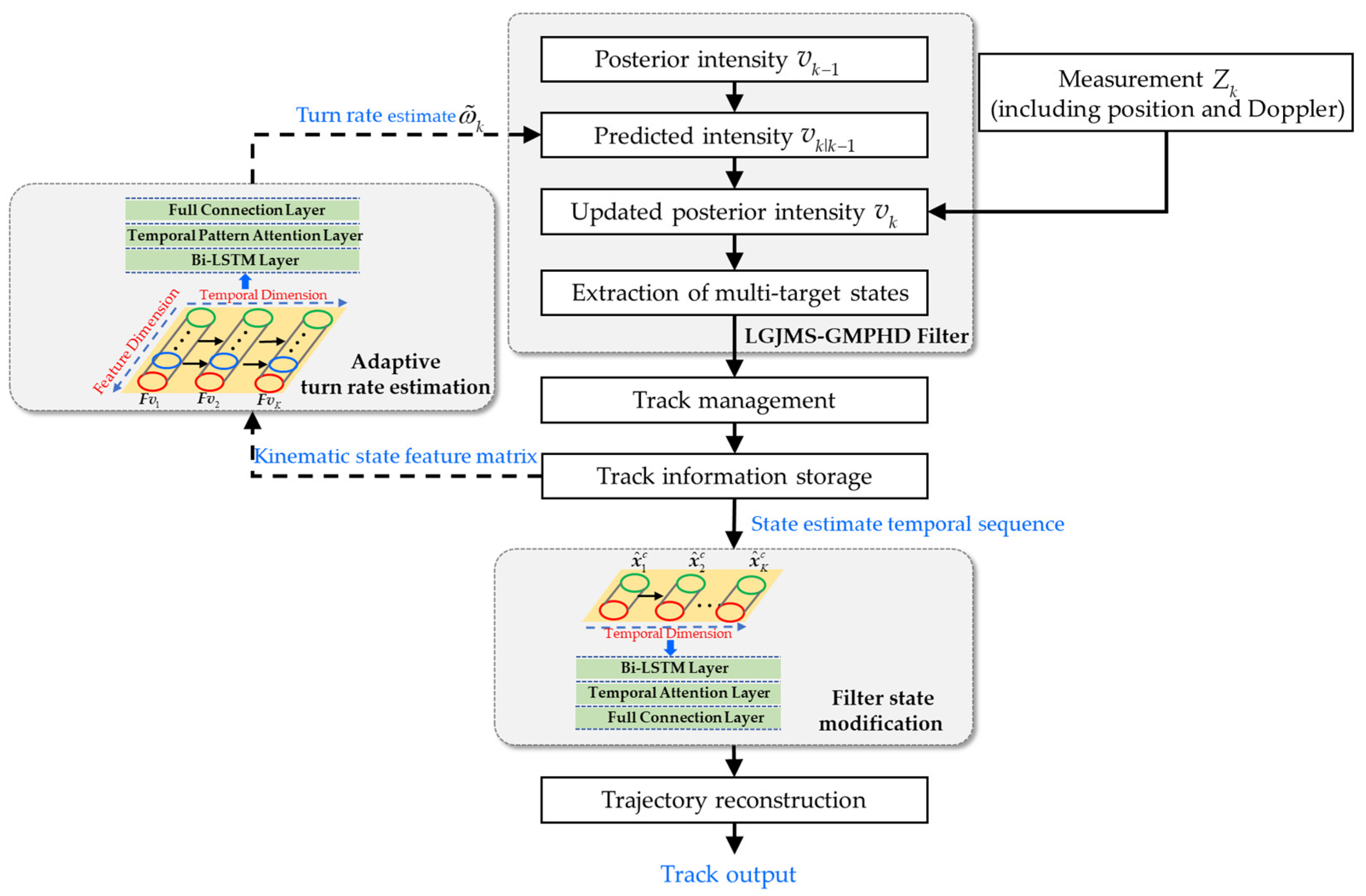
Therefore, a deep-learning-based multiple model tracking method is proposed to improve the adaptability of the LGJMS-GMPHD filter to complex maneuvering motions. The relevant flow diagram is shown in Figure 1. Firstly, the multi-target state estimate is obtained by the LGJMS-GMPHD filter. At the same time, track management [27] is performed to obtain the track labels of individual targets. Then, an adaptive turn rate estimation network is designed to realize the real-time estimation of the turn rate, and it is fed back to the filtering process to update the parameters of the CT model, thereby improving the matching degree of the filtering model. On this basis, a filter state modification network is designed to smooth the state estimates. Finally, a trajectory reconstruction is performed to implement the reconstruction of the track segments output by the network, and then the entire target track can be obtained.

3.1. Adaptive Turn Rate Estimation Network

In JMS, the determination of the turn rate parameter is the key point in the successful application of the CT model. However, in existing methods [15], the turn rate is estimated simply based on the filtering state estimates of the last frame. Additionally, the information dimension is less and the relationship between different variables is not fully utilized, so it is difficult to obtain an accurate estimate of the turn rate.

Deep learning provides an effective means to overcome the limitations of the traditional estimation method [28,29]. A proper network module design can mine more dimensional features, and a diverse set of trajectories can be constructed for network training, which contributes to obtaining more accurate parameter estimates for target trajectories with unknown maneuvering motions. Given all this, we designed an adaptive turn rate estimation network and integrated it into the LGJMS-GMPHD filtering process, thereby improving the tracking precision for CT maneuvering targets. The structure of the network is shown in Figure 2.

Based on the previous track information from time $K-w_a+1$ to $K$ obtained by the filtering process, the turn rate estimate at time $K$ can be obtained by the adaptive turn rate estimation network, where $w_a$ is the length of the sequence. The length of the sliding window is $s_a$. First, the feature matrix $Fv$, including multi-dimensional kinematic information, can be obtained and used as the input of the network. It is represented as follows:

$$F{v}_{K-w_a+1:K}\triangleq \left\{F{v}_{K-w_a+1},F{v}_{K-w_a+2},\cdots ,F{v}_K\right\}.$$

(31)

The feature vector at time $k$ is represented as follows:

$$F{v}_k=\left[{\hat{x}}_k,{\hat{y}}_k,{\widehat{\stackrel{.}{x}}}_k,{\widehat{\stackrel{.}{y}}}_k,{\stackrel{.}{r}}_k,x_k^m,y_k^m\right],\hspace{1em}k\in \left[K-w_a+1,K\right],$$

(32)

where ${\hat{x}}_k$ and ${\hat{y}}_k$ are the position estimates, and ${\widehat{\stackrel{.}{x}}}_k$ and ${\widehat{\stackrel{.}{y}}}_k$ are the velocity estimates. Meanwhile, based on the track labels, we can also obtain the measurements associated with the track, and then obtain the corresponding Doppler ${\stackrel{.}{r}}_k^m$, and positions $x_k^m$ and $y_k^m$.

The measurement precision of variables in the feature matrix $Fv$ is different. For example, the target Doppler usually has a higher precision than the position state estimates. Additionally, for each variable, the variation in the temporal dimension reflects the maneuvering characteristics of the target. Therefore, multi-perspective feature extraction is performed to mine more abundant features and improve the accuracy of the turn rate estimates. The temporal dimension feature of each variable is extracted by means of bidirectional long short-term memory (Bi-LSTM). Then, temporal pattern attention (TPA) [30] is introduced to determine the weights of different variables. The concrete implementation steps are as follows:

• Bi-LSTM

The Bi-LSTM structure is used to capture the temporal correlation information of the feature matrix $Fv$ at each previous time step. The structure of Bi-LSTM is shown in Figure 3. The output vector $h_{ik}$ corresponding to the $k$-th time point of the $i$-th Bi-LSTM is the element-wise sum of the forward and backward LSTM outputs ${\overrightarrow{h}}_{ik}$ and ${\overleftarrow{h}}_{ik}$ at the $k$-th time point, and is calculated as follows:

$$h_{ik}=\left[{\overrightarrow{h}}_{ik}\oplus {\overleftarrow{h}}_{ik}\right].$$

(33)

In the proposed adaptive turn rate estimate network, two Bi-LSTM layers are integrated, and the output hidden state matrix is represented as $H^A=\left\{h_{K-w_a+1}^a,h_{K-w_a+2}^a,\cdots ,h_K^a\right\}$, where $H^A\in {ℝ}^{m\times w_a}$, $m$ is the number of hidden units, and $h_k^a$ is the hidden state at time step $k$.

• Temporal pattern attention

For different features in $Fv$, the temporal patterns across multiple time steps and the weights are extracted by the temporal pattern attention module. First, the $f$ convolutional neural network (CNN) filters $C_i\in {ℝ}^{1\times w_a}$ are applied on the row vector of $H^A$ to extract temporal pattern features. The convolutional operations yield $H^C\in {ℝ}^{m\times f}$, where $H_{i,j}^C$ represents the convolutional value of the $i$-th row vector and the $j$-th filter. Formally, this operation is expressed as

$$H_{i,j}^C={\displaystyle \sum _{k=1}^{w_a}{H}_{i,k}\times C_{j,k}}.$$

(34)

Then, an attention mechanism is carried out. $v_K$ is calculated as a weighted sum of the row vectors of $H^C$ to capture the relational information between different variables. Defined below is the scoring function: $g:{ℝ}^k\times {ℝ}^m\mapsto ℝ$ to evaluate relevance:

$$g\left(H_i^C,h_K\right)={\left(H_i^C\right)}^{{\rm T}}{W}_a{h}_K,$$

(35)

where $H_i^C$ is the $i$-th row of $H^C$, and ${\mathit{W}}_a\in {ℝ}^{f\times m}$. The attention weight ${\alpha }_i$ is obtained as

$${\alpha }_i=sigmoid\left(g\left(H_i^C,h_K\right)\right).$$

(36)

The row vectors of $H^C$ are weighted by ${\alpha }_i$ to obtain the context vector $v_K\in {ℝ}^f$

$$v_K={\displaystyle \sum _{i=1}^n{\alpha }_i{H}_i^C}.$$

(37)

Finally, integrating $v_K$ and $h_K$ to yield the turn rate estimate:

$${h^{\prime }}_K=W_h{h}_K+W_v{v}_K,$$

(38)

$${\tilde{\omega }}_K=W_{h^{\prime }}{h^{\prime }}_K,$$

(39)

where $h_K$, $h_K^{\prime }\in {ℝ}^m$, $W_h\in {ℝ}^{m\times m}$, $W_v\in {ℝ}^{m\times f}$, $W_{h^{\prime }}\in {ℝ}^{n\times m}$, and ${\tilde{\omega }}_K\in {ℝ}^n$ is the turn rate estimate.

In the training stage, the root mean square error (RMSE) is used as the loss function:

$$\mathcal{L}=\sqrt{{\displaystyle \sum _{k=K-w_a+1}^K{\left({\tilde{\omega }}_k-{\omega }_k\right)}^2}},$$

(40)

where ${\omega }_k$ is the true turn rate. The model is trained by minimizing (40) and is optimized through the adaptive moment estimation (Adam) algorithm [31] over the training datasets.

3.2. Filter State Modification Network

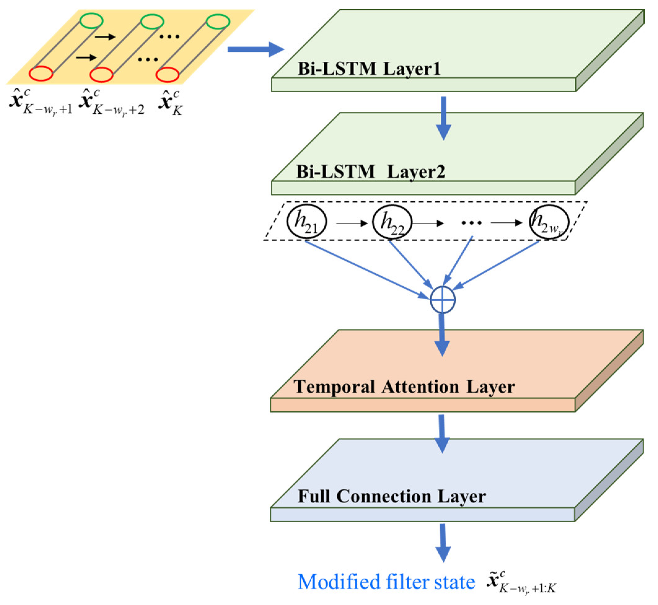
For strong maneuvering targets, the motion switches between multiple models with uncertainty. The multiple model filtering state estimates have a delay in their response to target maneuvering, resulting in the degradation of the tracking performance. Therefore, a filter state modification network is designed here to smooth the state estimates and advance the tracking precision. The diagram is shown in Figure 4.

The state estimate of each target obtained by the LGJMS-GMPHD filter is first cropped into a state vector of uniform length $w_r$, and the length of the sliding window is $s_r$. It is used as the input of the network and is represented as follows:

$${\hat{x}}_{K-w_r+1:K}^c\triangleq \left\{{\hat{x}}_{K-w_r+1}^c,{\hat{x}}_{K-w_r+2}^c,\cdots ,{\hat{x}}_K^c\right\},$$

(41)

where ${\hat{x}}_k^c={\left[\begin{array}{cc}{ \hat{\mathit{x}}}_k& { \hat{\mathit{y}}}_k\end{array}\right]}^{\mathit{T}},\hspace{1em}k\in \left[K-w_r+1,K\right]$ is the state vector including position estimates.

The variation of the state estimate vector along the temporal dimension can reflect the maneuvering characteristics of the target. Therefore, in the proposed filter state modification network, Bi-LSTM is also applied to extract the temporal correlation information in the forward and reverse directions. In addition, temporal attention (TA) [32] is integrated to weight the hidden state vectors at each time step.

The specific implementation of each module is described as follows.

• Bi-LSTM

Two Bi-LSTM layers are integrated to capture the temporal correlation information of state vector ${\hat{x}}_{K-w_r+1:K}^c$ at each previous time step. The output hidden state matrix is represented as $H^R=\left\{h_{K-w_r+1}^R,h_{K-w_r+2}^R,\dots ,h_K^R\right\}$, where $H^R\in {ℝ}^{m\times w_r}$, $m$ is the number of hidden units, and $h_k^R$ is the hidden state at time step $k$.

• Temporal attention

The hidden state matrix after the temporal attention module is represented as $H^{ta}=\left\{h_{K-w_r+1}^{ta},h_{K-w_r+2}^{ta},\dots ,h_K^{ta}\right\}$, $H^{ta}\in {ℝ}^{m\times w_r}$, which is obtained by weighting $H^R$ at each time step. The weight at time $k$ is represented as ${\alpha }_k^{ta}$ and is calculated as follows:

$$M_k=\tanh \left(h_k^R\right),$$

(42)

$${\alpha }_k^{ta}=\frac{\exp \left({\epsilon }_k^T{M}_k\right)}{{\displaystyle \sum _{j=1}^{w_r}\exp \left({\epsilon }_j^T{M}_j\right)}},$$

(43)

$$h_k^{ta}=\tanh \left({\alpha }_k^{ta}{h}_k^R\right),$$

(44)

where ε_k is a trained parameter vector and the dimension is $m$. Then $H^{ta}$ passes through the full connection layer to obtain the modified filter state output:

$${ \tilde{x}}_{K-w_r+1:K}^c=W^{fc}{H}^{ta}+b^{fc},$$

(45)

where W^fc and $b^{fc}$ represent the weight and bias matrix of the full connection layer, respectively.

In the training stage, the loss function is:

$$\mathcal{L}=\sqrt{{\displaystyle \sum _{k=K-w_r+1}^K{\left({ \tilde{x}}_k^c-{\mathit{x}}_k^c\right)}^2}},$$

(46)

where ${ \tilde{x}}_k^c$ is the modified filter state estimate and ${\mathit{x}}_k^c$ is the ground-truth of the trajectory. The model is trained by minimizing (46) and is optimized through the Adam algorithm over the training datasets.

3.3. Trajectory Reconstruction

In the proposed deep-learning-based multiple model tracking method, the historical track information of the target is clipped into segments of appropriate length and used as the input of the deep learning network. Therefore, to obtain the state estimate of the entire trajectory, the modified trajectory segments ${\tilde{x}}_{K-w_r+1:K}^c$ output from the filter state modification network need to be connected through a reconstruction step [23].

When the length of a trajectory segment is $w_r$ and the sliding window is s_l, the overlap region of the adjacent segments is from $K-w_r+s_l+1$ to $K$. The value of the target states in the overlap region is the average of the two adjacent segments, and the state parameters remain constant for non-overlapping regions. The above process is repeated to complete the reconstruction of trajectory segments at each time, and the entire target trajectory can be obtained.

4. Network Parameter Design and Performance Analysis

To guarantee the flexibility of the designed deep learning network in real scenarios, a training dataset, including trajectories with different positions, speeds, turn rates, and various maneuvering modes, was constructed. In addition, process noise and measurement noise were added to simulate the target trajectories more realistically. Meanwhile, based on the estimation accuracy of the test dataset, the suitable network structure, network parameters, and input sequence length were designed. Finally, we verified the effectiveness of the two network modules in improving the tracking precision in relation to complex maneuver targets.

For the sake of convenience, in the comparisons of results presented below, LGJMS-GMPHD is abbreviated as GMPHD. After introducing adaptive turn rate estimation, it is denoted as GMPHD-ATN, and after introducing filtering state modification, it is denoted as GMPHD-ATN-FMN.

4.1. Dataset Preparation

4.1.1. Parameter Design

• Target trajectory parameters

We designed five groups of maneuvering trajectories, as shown in

Table 1. The kinematic parameters of the target trajectory.

Group Index	Initial Velocity (m/s)	Turn Rate
		Stage 1	Stage 2	Stage 3	Stage 4
1	[−60, 60]	0	${\omega }_1$	0	/
2	[−40, 40]	0	${\omega }_2$	0	/
3	[−60, 60]	0	${\omega }_1$	${\omega }_2$	0
4	[−60, 60]	0	${\omega }_1$	${\omega }_1$	0
5	[−40, 40]	0	${\omega }_2$	${\omega }_1$	0

, including different turn rate parameters. A turn rate equal to $0°/s$ represents the CV stage and a non-$0°/s$ rate represents the CT stage. Meanwhile, two groups of turn rate intervals were designed: ${\omega }_1\in \left[-8°/s,8°/s\right]$ represents a slow turn and ${\omega }_2\in \left[-15°/s,-8°/s\right]\cup \left[8°/s,15°/s\right]$ represents a fast turn. In addition, the durations of different motion stages are different. Specifically, CV is 20–25 s, ${\omega }_1$ is 10–50 s, and ${\omega }_2$ is 8–20 s. For each group of trajectories in the training datasets, the kinematic parameters were uniformly extracted according to Table 1.

• Filter parameters

For the LGJMS-GMPHD filter process, $\mu =1$ is the CV model and $\mu =2$ is the CT model. The switching between the motion models is given by the Markov transition probability matrix as

$$\left[{\tau }_{k|k-1}\left({\mu }_k|{\mu }_{k-1}\right)\right]=\left[\begin{array}{cc}0.9& 0.1\\ 0.1& 0.9\end{array}\right].$$

(47)

For simplicity, we assume that the probability of target survival and detection is constant. $p_{S,k|k-1}=0.99$ and $p_{D,k}=0.98$ are assumed for models $\mu =1,2$. Additionally, the interval between the samples is $T=1 s$. The standard deviation of process noise ${\sigma }_v=1m/s^2$ and the standard deviation of measurement noise ${\sigma }_R=10m$.

4.1.2. Dataset Construction

• Training and validation datasets

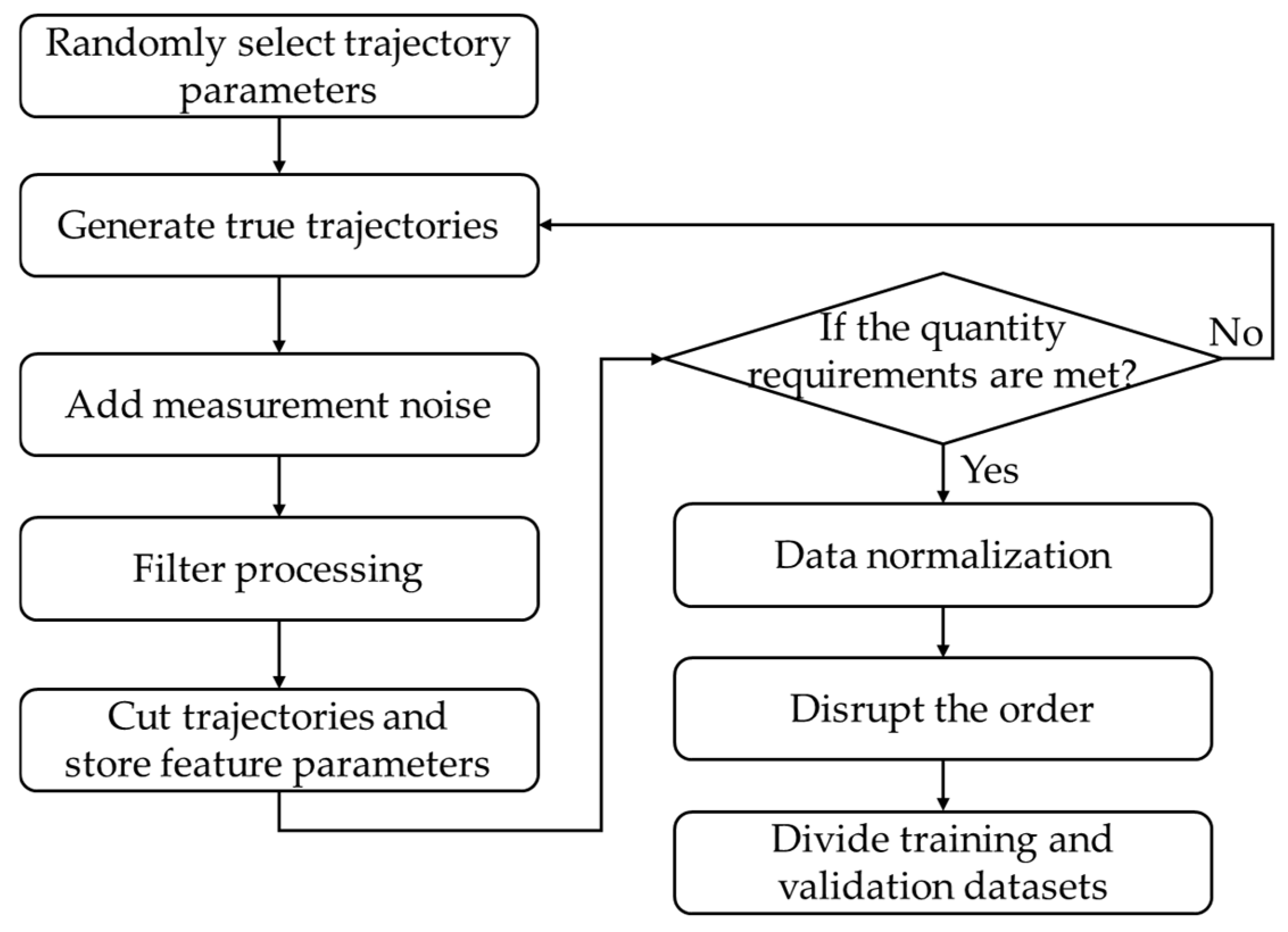
The construction of the datasets for the two networks is summarized in the flowchart shown in Figure 5. The details are described as follows:

(a)

The kinematic parameters from Table 1 are randomly selected to generate real target trajectories.

(b)

Measurement noise is added and target measurements are obtained.

(c)

The LGJMS-GMPHD filter process is performed to obtain the state estimate, where the turn rate of CT model is calculated via a physical definition method to obtain the datasets of the adaptive turn rate estimate network, and the true value is used to obtain the datasets of the filter state modification network.

(d)

The trajectories are clipped to segments of uniform length. For the adaptive turn rate estimation network, the feature matrix $Fv$ defined in (31) is stored. For the filter state modification network, the position state estimate ${\hat{\mathit{x}}}^c$ defined in (41) is stored.

(e)

Data normalization is performed based on min-max scaling.

(f)

The order is disrupted and the training and validation datasets are divided.

In this paper, the number of trajectory segments in the training and validation datasets for the two networks was 300,000 and 60,000, respectively. In the training procedure, the learning rate was set to 10⁻⁴, the batch size was 100 samples, and the training epoch was 300.

• Test datasets

Based on the trajectory parameters shown in Table 1, 100 maneuvering trajectories were constructed for each group to verify the effectiveness of each module in the proposed method in improving tracking performance.

4.2. Network Module Parameter Design

4.2.1. Adaptive Turn Rate Estimation Network

The network structures, parameters, and input sequence length were validated based on the five groups’ trajectories with different maneuvering forms in the test datasets. The evaluation criterion is the RMSE of turn rate estimate and defined as follows:

$${\sigma }_{\omega }\left(k\right)=\sqrt{\frac{1}{N}{\displaystyle \sum _{i=1}^N{\left(\hat{\omega }\left(k\right)-\omega \left(k\right)\right)}^2}}$$

(48)

where $\hat{\omega }\left(k\right)$ is the output of the adaptive turn rate estimation network, and $\omega \left(k\right)$ is the true value. $N$ is the number of simulations.

• Network structure

The number of Bi-LSTM layers and the module effectiveness were verified based on the RMSE of the turn rate estimate, as shown in

Table 2. RMSE of different network structures (units: degree).

Group Index	Network Structure
	One Bi-LSTM Layer	Two Bi-LSTM Layers	Three Bi-LSTM Layers	Four Bi-LSTM Layers	Two Bi-LSTM Layers + TPA
1	0.90	0.76	0.76	0.77	0.55
2	2.06	1.63	1.56	1.45	0.92
3	1.67	1.37	1.35	1.23	0.74
4	1.29	1.23	1.24	1.23	0.91
5	1.78	1.48	1.48	1.42	1.02

. Here, we set the number of hidden units of the Bi-LSTM to 64, the sequence length to 10, and the sliding window to 1. Compared to one Bi-LSTM layer, two Bi-LSTM layers can produce a higher accuracy, but the improvement is not significant as the number of layers continues to increase. Therefore, we set the number of Bi-LSTM layers as two. After the TPA module was introduced, it can be seen from the last column that the estimation error was greatly reduced. Especially for the second group, the RMSE was reduced by 0.71°, which verifies the effectiveness of the TPA module.

• Network parameters

After the network structure was determined, we analyzed the influence of the number of hidden units of the Bi-LSTM layers on the performance. The RMSE of the turn rate estimates with different numbers of hidden units for the Bi-LSTM layers is shown in

Table 3. RMSE of different network parameters (units: degree).

Group Index	Number of Hidden Units
	32	64	96	128
1	0.62	0.55	0.55	0.56
2	1.06	0.92	0.86	0.88
3	0.82	0.74	0.70	0.68
4	0.97	0.91	0.90	0.88
5	1.09	1.02	1.04	1.04

. Here, we set the sequence length to 10 and the sliding window to one. As the number of hidden units increased, the RMSE decreased, but the reduction was not significant for 64, 96, and 128. Therefore, considering operational efficiency and estimation precision comprehensively, we set the number of hidden units to 64.

• Sequence length

Long sequences generally contain more abundant feature information, but this also degrades the real-time performance and increases the difficulty of network training. Therefore, we analyzed the influence of input sequence length on the estimate precision of the network. Here, we set the number of hidden units to 64 and the sliding window to one. The RMSE comparisons for different sequence length are shown in

Table 4. RMSE of different input sequence lengths (units: degree).

Group Index	Sequence Length
	6	8	10	12	14
1	0.64	0.60	0.55	0.54	0.58
2	0.98	0.87	0.92	0.84	0.86
3	0.80	0.76	0.74	0.69	0.72
4	1.04	0.98	0.91	0.88	0.92
5	1.13	1.07	1.02	1.00	1.01

. When the sequence length increased from 6 to 12, the RMSE of the turn rate estimate decreased gradually. However, when the length was 14, the RMSE increased slightly compared with 12. Therefore, we set the input sequence length of the turn rate estimation network as 12.

4.2.2. Filter State Modification Network

The network structure, parameters, and input sequence length were validated based on the testing datasets. The evaluation criterion was the RMSE and was defined as follows:

$${\sigma }_M\left(k\right)=\sqrt{\frac{1}{N}{\displaystyle \sum _{i=1}^N\left({\left({\hat{x}}_k-x_k\right)}^2+{\left({\hat{y}}_k-y_k\right)}^2\right)}}$$

(49)

where ${\hat{x}}_k$ and ${\hat{y}}_k$ represent the output of the network, and $x_k$ and $y_k$ are the real values; $N$ is the number of simulations.

• Network structure

Comparisons of the RMSE of different network structures are shown in

Table 5. RMSE of different network structures (units: m).

Group Index	Network Structure
	One Bi-LSTM Layer	Two Bi-LSTM Layers	Three Bi-LSTM Layers	Four Bi-LSTM Layers	Two Bi-LSTM Layers + TA
1	11.96	11.62	12.52	13.13	11.28
2	10.23	9.93	9.99	10.02	9.88
3	11.61	11.20	12.68	13.07	10.66
4	11.71	11.21	12.91	13.43	10.84
5	11.41	10.86	10.98	10.99	10.82

. Here, we set the number of hidden units to 64, the length of input sequence to 15, and the sliding window to five. First, when the number of Bi-LSTM layers increased from one to two, the output precision of the network was obviously improved. However, when the number of layers increased to three and four, the RMSE of groups 1, 3, and 4 increased instead; that is, the network was overfitted. Therefore, we set the number of Bi-LSTM layers to two. After the temporal attention module was introduced, as shown in the last column in Table 5, the RSME was further reduced. Especially for groups 1, 3, and 4, the reduction was remarkable, which verifies the effectiveness of the TA module.

• Network parameters

The RMSE of test datasets for different numbers of hidden units is shown in

Table 6. RMSE of different network parameters (units: m).

Group Index	Number of Hidden Units
	32	64	96	128
1	11.46	11.28	11.19	11.32
2	9.91	9.88	9.77	9.79
3	10.81	10.66	10.73	10.98
4	11.01	10.84	10.79	10.95
5	10.85	10.82	10.72	10.71

. Here, we set the length of the input sequence to 15 and the sliding window to five. First, with the increase in the number of hidden units, the network performance was improved, but the increase was not obvious. The RMSE for 64 hidden units was reduced by about 0.2 m compared with that for 32 hidden units. Compared with 64, the performance improvement for 96 and 128 hidden units was about 0.1 m. Meanwhile, for groups 1–4, overfitting also occurred when the parameter was 128. Hence, we set the number of hidden units to 64.

• Sequence length

The influence of the input sequence length on the precision of the filter state modification network was analyzed. Comparisons of the RMSE of the testing datasets are shown in

Table 7. RMSE of different input sequence lengths (units: m).

Group Index	Sequence Length
	8	10	12	14	15	16
1	12.29	12.08	11.81	11.30	11.28	11.71
2	10.37	10.52	10.36	10.02	9.88	9.97
3	11.67	11.71	11.34	11.10	10.66	10.89
4	12.16	11.70	11.55	11.22	10.84	11.21
5	11.36	11.32	11.24	11.16	10.82	11.06

. Here, we set the number of hidden units to 64 and the sliding window to five. Horizontally, for each group of test trajectories, the RMSE decreased with the increase in the sequence length. However, when the sequence length was 15, the error was at its minimum, and when the sequence length increased to 16, the performance slightly decreased. Therefore, we set the input sequence length to 15.

4.3. Network Module Performance Validation

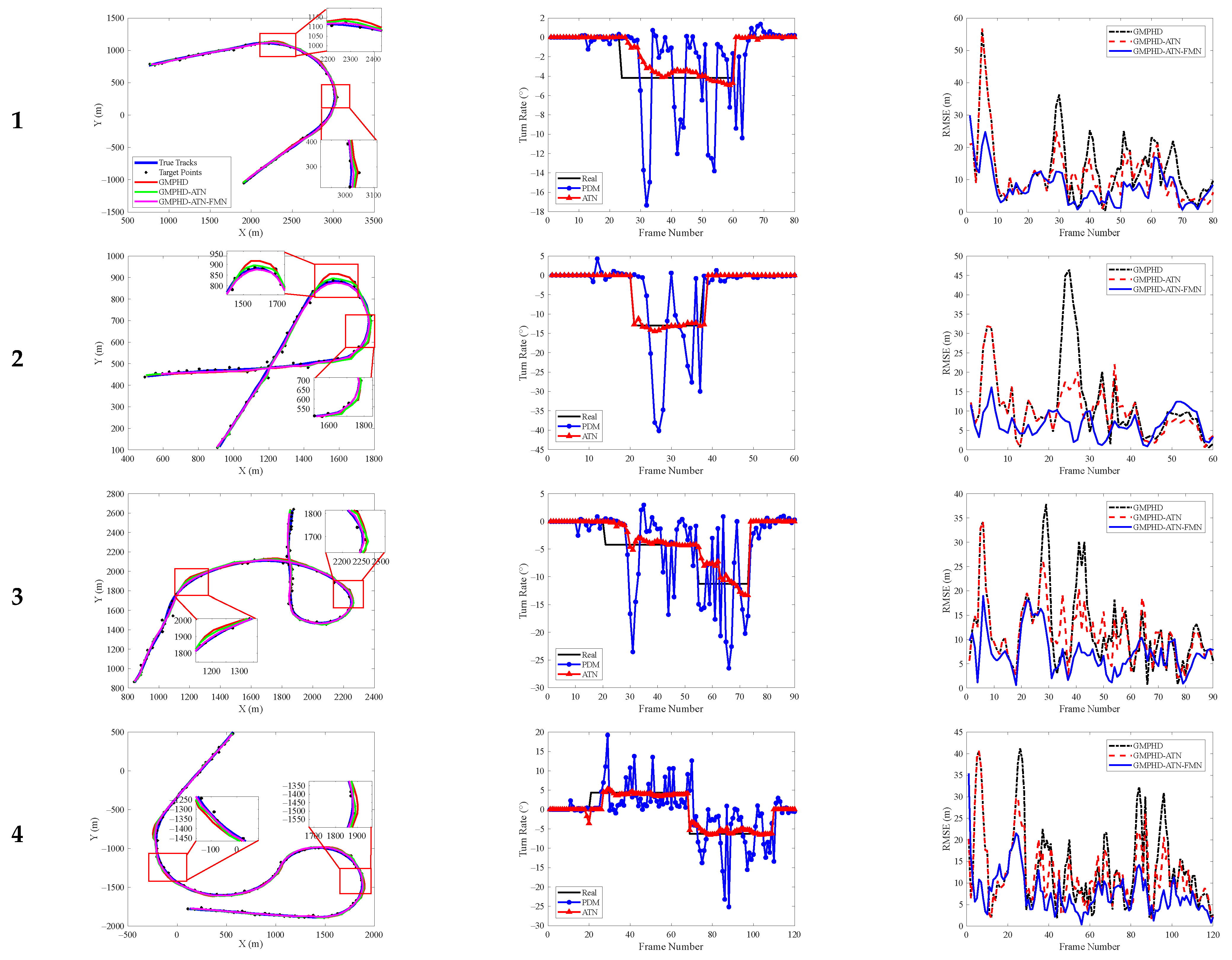
In this section, five groups of target trajectories with different maneuvering modes in the testing datasets were extracted to verify the validity of the two network modules in the proposed deep-learning-based multiple model tracking method. To show the result comparisons more intuitively, we extracted a target trajectory from each group of maneuvering modes, and the comparison of single simulation results is shown in Figure 6. The first column represents the comparison of the tracking results, the second column represents the comparison of the turn rate estimation results, and the third column represents the comparison of the tracking errors.

• Effects of the adaptive turn rate estimation network

For the traditional physical definition method, only the filtering state estimates in the last frame were used. In the maneuvering phase, the estimation error of the turn rate was large and fluctuated greatly, which led to a decrease in the tracking precision. Especially for the strong maneuvering trajectory with a large turn rate, for example, the second target performed the turning motion with the parameter $\omega =-13°/s$ between frames 20 and 38, and the tracking RMSE in the corresponding period increased rapidly. For the proposed adaptive turn rate estimation network, multi-frame kinematic features can be utilized and more complex logical relationships between different variables can be extracted, which contributes to obtaining more accurate estimates of turn rates, as shown by the red curve in Figure 6b. Although the estimation error in the maneuvering phase was slightly larger than that in the non-maneuvering phase, the performance gradually became stable after several frames. The corresponding tracking results are indicated by the red curve in Figure 6c. Compared with the GMPHD filter, our method can effectively reduce the tracking error in the turn maneuvering phase.

• Effects of the filter state modification network

As can be seen from the tracking results in Figure 6a and the tracking error curve in Figure 6c, an accurate estimate of the turn rate can improve the tracking performance to a certain extent. However, there is uncertainty in the switching of target motion models, resulting in large tracking errors. The filter state modification network can smooth the target state estimates that are produced by the GMPHD filter. As shown in Figure 6a, the tracking result of the purple curve is smoother than those of the red and green curves. Additionally, it can also be seen in Figure 6c that the RMSE corresponding to the blue curve greatly decreased during the turning maneuver phase.

Furthermore, from the tracking result comparisons of all trajectories in the testing datasets shown in Figure 7, it can be concluded that the proposed method has strong adaptability to multiple maneuvering modes and can effectively enhance the tracking precision of complex maneuvering targets.

5. Simulations and Experimental Results

In this section, the adaptability of the proposed method to the multiple maneuvering target tracking in a cluttered environment is demonstrated.

5.1. Simulations

5.1.1. Simulation Scenario and Parameters

Multiple maneuvering targets in a cluttered environment were constructed to verify the tracking performance of the proposed method. The filter parameter design was the same as that presented in Section 4.1.1. In addition, the detected measurements were immersed in clutter, which can be modelled as a Poisson RFS $K_k$ with intensity

$${\kappa }_k\left(z\right)={\lambda }_{c}V\mathcal{U}\left(z\right)$$

(50)

where $\mathcal{U}(·)$ is the uniform density over the surveillance region, $V=1.6\times {10}^7{m}^2$ is the ‘volume’ of the surveillance region, and ${\lambda }_c=3.2\times {10}^{-6}{m}^{-2}$ is the average number of clutter returns per unit volume.

We designed five target trajectories, representing the five maneuvering forms shown in Table 1 respectively, and the trajectory parameters of each target are shown in

Table 8. Target trajectory parameters.

Index	Initial State	$\mathbf{Turn} \mathbf{Rate} \left(°/\mathbf{s}\right)$
1	[500 m; 20 m/s; 523 m; −25 m/s]	1~24 s	25~57 s		58~84 s
		0	−7		0
2	[243 m; −35 m/s; 266 m; −20.4 m/s]	1~21 s	22~33 s		34~55 s
		0	−10.4		0
3	[941 m; −27.4 m/s; 737 m; 35.5 m/s]	1~21 s	22~70 s	71~82 s	83~110 s
		0	5.2	−10.6	0
4	[1000 m; 15 m/s; 1300 m; −20 m/s]	1~25 s	26~49 s	50~94 s	95~116 s
		0	2.9	−6.9	0
5	[109 m; −30 m/s; 620 m; −30 m/s]	1~23 s	24~33 s	34~54 s	55~74 s
		0	13.7	−7.8	0

. The simulation scenario is shown in Figure 8.

5.1.2. Result Comparisons

Based on the simulation scenarios shown in Figure 8, the tracking performance of the proposed method was verified, and the optimal subpattern assignment (OSPA) metric [33] was adopted to evaluate the performance of multi-target tracking. After 100 Monte Carlo simulation runs, the OSPA distance comparison is shown in Figure 9, and the turn rate estimate error is shown in Figure 10.

First, from 25–32 s and 71–82 s, targets 2, 3, and 5 all contained fast turning maneuvers with the parameter ${\omega }_2$, and the OSPA distance of the GMPHD filter increased dramatically. For GMPHD-ATN, it did not show a large fluctuation, and compared with the GMPHD filter, the maximum reduction was about 12 m, which verifies the importance of turn rate estimate accuracy for the stable tracking of strong maneuvering targets. Additionally, for the GMPHD-ATN-FMN, the introduction of the filter state modification network module was able to smooth the state estimate. Therefore, the tracking precision was further significantly improved in the entire tracking stage, and the performance was improved significantly in the strong maneuvering phase. Specifically, in the weak maneuvering stage, such as 35–70 s, the maximum reduction of OSPA distance was about 4 m, whereas in the strong maneuvering stage, such as 25–32 s, the maximum reduction was about 7.5 m.

Figure 11 shows comparisons of the tracking results obtained in a single simulation. The estimate results of the turn rate for the five targets are shown in Figure 12. For target 5, the large estimate error of the turn rate in GMPHD led to a mismatch in the filtering parameters, and the track was broken in area 3. After introducing the adaptive turn rate estimation process, as shown in Figure 12, more accurate estimates of the turn rate can be obtained. Although the estimate error increased slightly when the motion model switched, after several frames the error gradually decreased. As indicated by the green curve in Figure 11, the matched filtering parameters were able to effectively improve the tracking precision and avoid track breakages in the maneuvering stage. Additionally, as shown by the purple curve in Figure 11, the filter state modification process can smooth the trajectory and output higher quality maneuvering target tracks.

5.2. Experimental Data Validation

5.2.1. Experimental Scenarios and Parameters

In this section, the tracking performance of the proposed method is further verified based on experimental field data. The experimental equipment is a phased array radar working in the Ku band. The sample interval is 6 s. In the experiment, the flight height of a small UAV (DJI Matrice 600) is approximately 200 m with CT maneuvers. The experimental scenario is shown in Figure 13.

5.2.2. Result Comparisons

After the echo data collected by the radar were processed by constant false alarm rate detection, measurements of the area where the UAV was located could be obtained. To verify the tracking performance in the multiple targets scenario, we combined two sets of measurements of the single UAV target into one set.

Figure 14 shows the tracking result comparisons. Firstly, for the GMPHD with unknown turn rate parameters, the mismatch in the model parameter resulted in track breakages at the turning position. For the GMPHD-ATN, the track quality was significantly improved. Additionally, as shown in Figure 14c, after introducing filter state modification processing, the tracking result was smoothed, and the precision of the state estimate was effectively improved. Therefore, the tracking results of real UAV observation data verify the rationality of the parameters of the constructed training datasets, and the proposed method demonstrated its adaptability to practical scenarios with detection and measurement noise uncertainties.

5.2.3. Computational Complexity

For a fair comparison, the computational efficiency of all algorithms was tested on an Intel Xeon E5-2680 CPU at 2.4 GHz. For the adaptive turn rate estimation network, the testing runtime per iteration was 2 ms, and for the filter state modification network, the testing runtime per iteration was 4 ms. Although the training of the deep neural network was time consuming, its implementation in practice is highly efficient because the calculations are mainly matrix multiplications and element-wise operations. Therefore, the proposed method can ensure the real-time performance of the tracking process.

6. Discussion

The RFS-based filter incorporating the jump Markov system approach is an effective method for multiple maneuvering target tracking in cluttered environments. However, UAV targets have strong maneuverability and their trajectory forms are diverse, presenting unknown motion model parameters and uncertain model switching. The preset parameters of filter models are difficult to match to the time-varying target motion, leading to a serious decline in tracking performance. Therefore, within the framework of the LGJMS-GMPHD filter, we proposed a deep-learning-based multiple model tracking method to improve maneuvering adaptability.

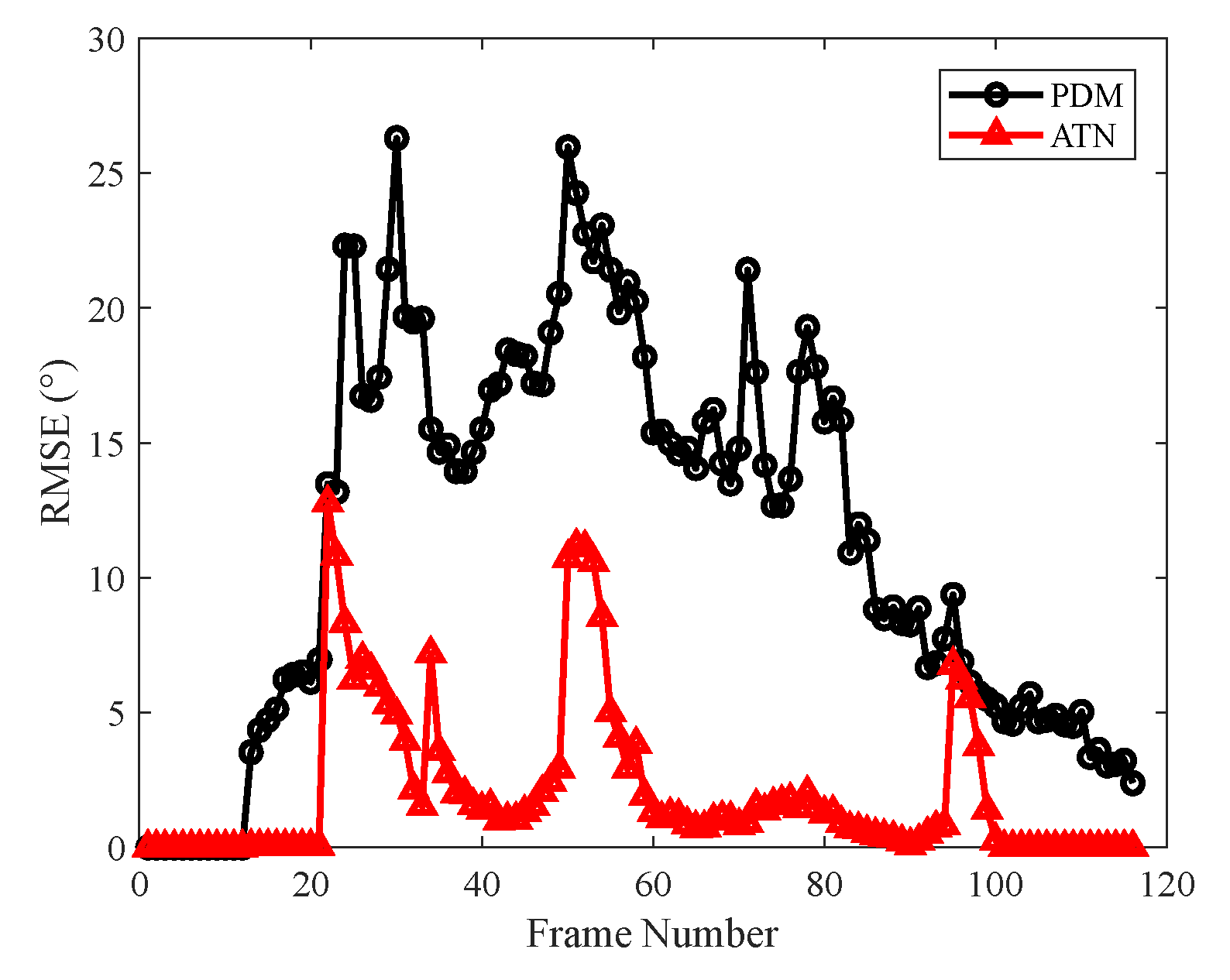
The simulation results indicated that the traditional LGJMS-GMPHD filter has a low tracking precision and the track is prone to breaking in scenarios involving complex maneuvering targets. As shown in Figure 12, for the PDM, the estimation error of the turn rate was large and fluctuated greatly in the maneuvering phase as only the filtering state estimate in the last frame was considered, whereas the proposed adaptive turn rate estimation network made use of multiple dimensions of kinematic features and extracted the relationship between different features. As shown in the red curve in Figure 12, a more accurate estimation of turn rate can be obtained, which helps to improve the matching degree of the CT model in the filter. 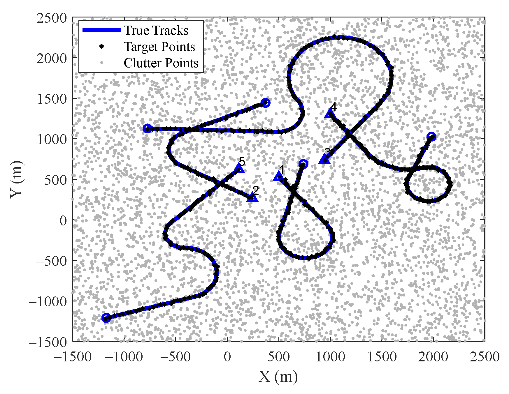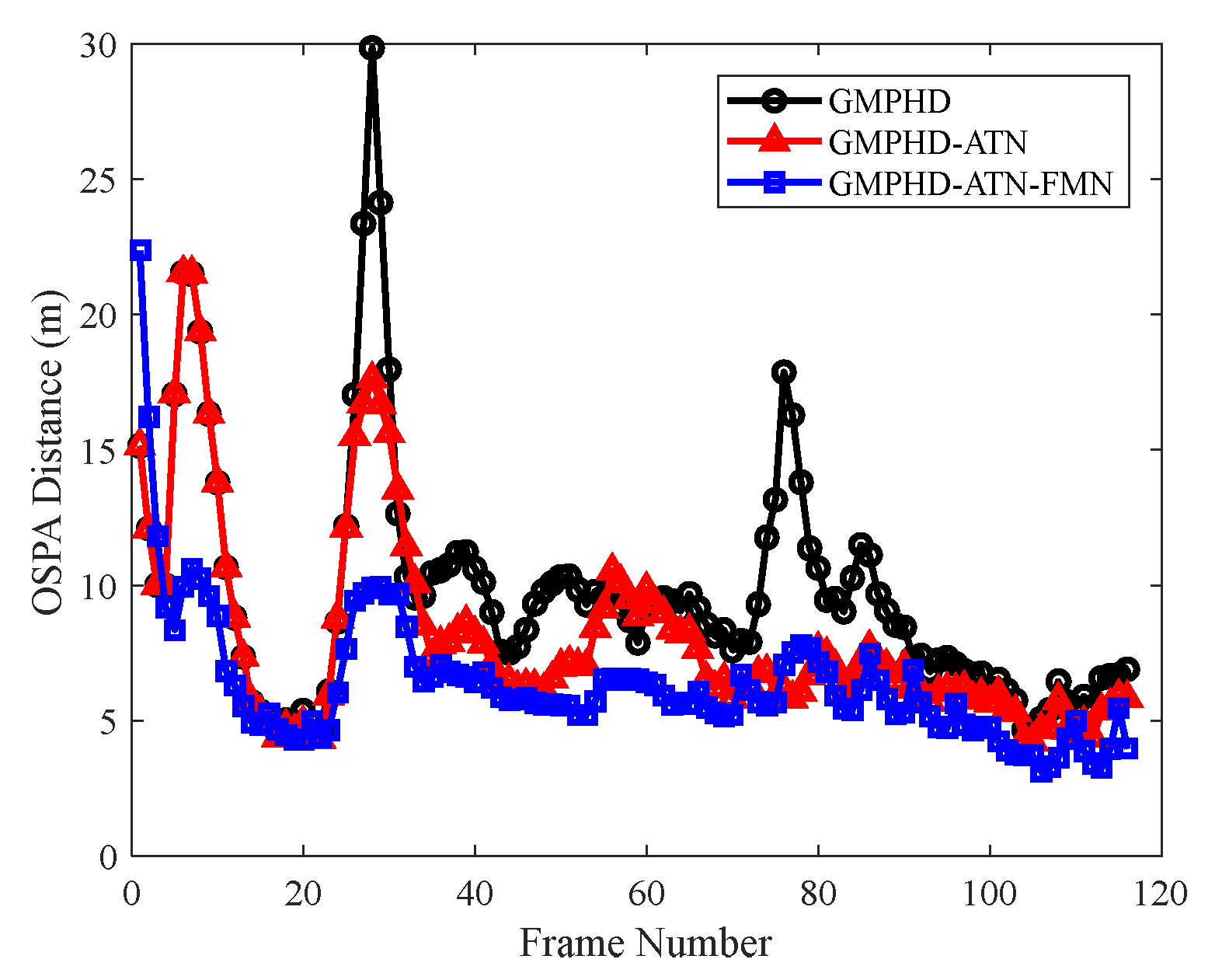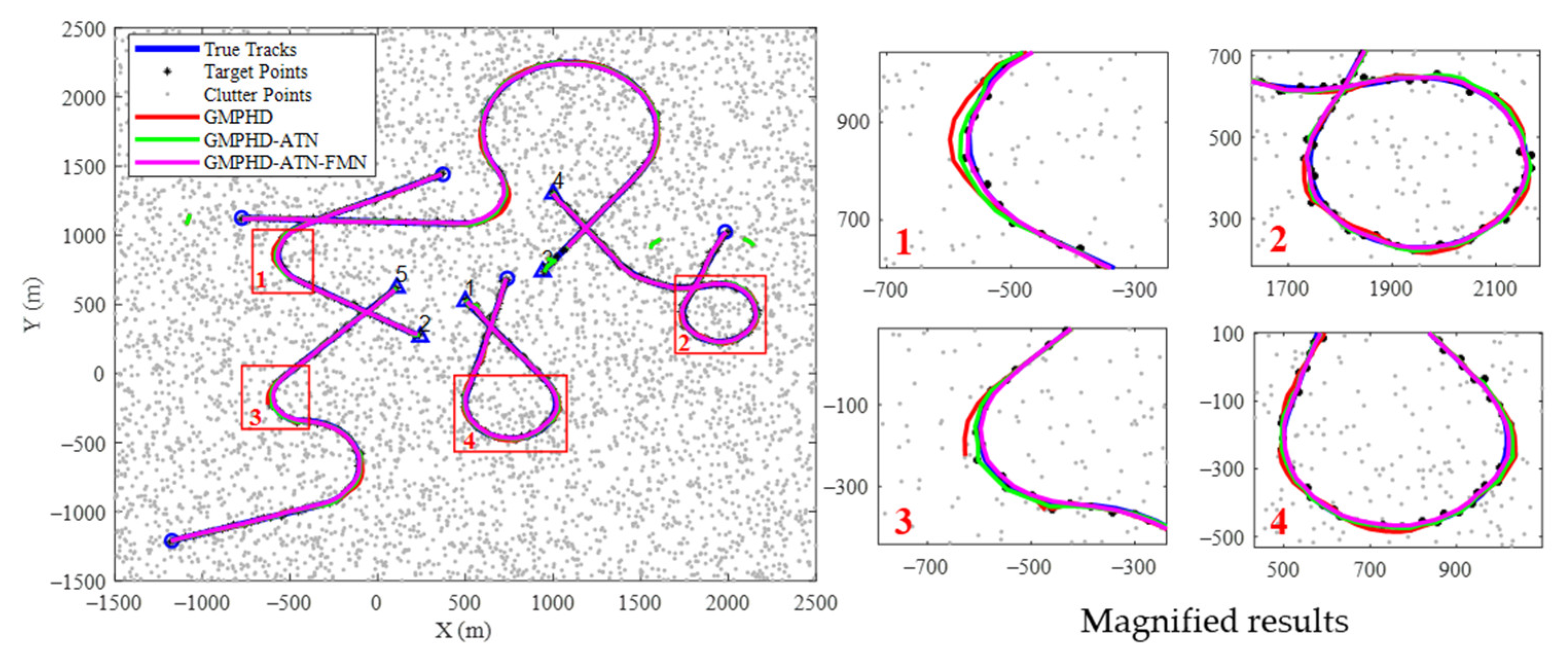Therefore, as shown in Figure 9, compared with the GMPHD filter, the OSPA distance of GMPHD-ATN was greatly reduced, and the tracking results shown in Figure 11 indicate that track continuity was optimized.

Another reason for poor tracking performance is the uncertainty of motion model switching. Smoothing results in better estimates for target states by means of a time delay. However, as described in [21], longer lags do not yield better estimates of the current state because the temporal correlations cannot be extracted. Moreover, backward smoothing is still model-based, which cannot address the substantive problem of tracking performance degradations due to model switching. Deep neural networks have a strong capability of fitting any mapping, providing an effective way to handle target motion uncertainty. However, the LSTM-based deep recurrent neural network in [24] only considered CV and CA motions, and is not suitable for the scenario of multiple maneuvering targets in the CT model. However, in the proposed filter state modification network, the state estimates output by the LGJMS-GMPHD filter were used as the input, and the temporal correlation information of the state vector was captured, with the ability to handle complex maneuvering motions. Hence, as shown in Figure 9, the tracking precision was improved in the entire tracking stage, especially in the strong maneuvering phase. The tracking results, shown in Figure 11, demonstrated that the track was smoothed and the track quality was improved. 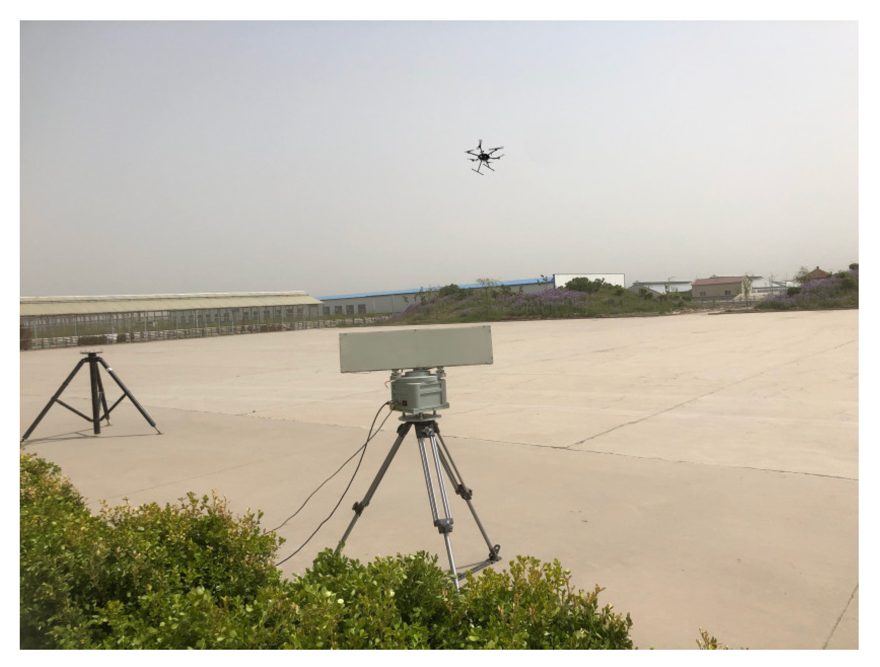Moreover, based on the tracking error comparisons of test datasets, shown in Figure 7, it can be concluded that the proposed method has strong adaptability to different maneuvering forms. The experimental data processing results indicate that the parameters of the training dataset designed in this paper can adapt to practical scenarios, and the method can effectively enhance the track quality of real UAV targets.

However, in this paper, we assumed that the clutter rate was known and remained constant. In future research, more complex detection environments, such as a time-varying clutter rate and detection uncertainty, will be considered. Furthermore, we will also consider extending the proposed method to group target tracking.

7. Conclusions

In this paper, we have proposed a deep-learning-based multiple model tracking method. The adaptive turn rate estimation network employs multi-frame and multi-dimensional kinematic information to improve the accuracy of the turn rate estimates for a maneuvering target with CT motion, thereby enhancing the consistency with the filtering model. Additionally, the filter state modification network uses the temporal features of the multi-frame state estimate to achieve the smoothing of target state estimates, thereby circumventing the large tracking errors caused by uncertain motion model switching. To ensure the applicability of the algorithm, in the training datasets, we designed five switching modes of the movement model. Therefore, the proposed method is suitable for practical maneuvering movements: (i) from CV to CT, (ii) from CT with ${\omega }_1$ to CT with ${\omega }_2$, and (iii) from CT to CV. In the end, based on the simulation results of multiple maneuvering target tracking in cluttered environments, it can be concluded that the proposed method can obtain accurate turn rate estimates and output high-quality tracks, and the performance improvement is especially significant in the maneuvering phase. Moreover, for the real UAV observation scenario with measurement noise and detection uncertainties, the proposed method can output more stable and smooth trajectories, which verifies its applicability in real scenarios.