A Sensor Bias Correction Method for Reducing the Uncertainty in the Spatiotemporal Fusion of Remote Sensing Images

Abstract

With the development of multisource satellite platforms and the deepening of remote sensing applications, the growing demand for high-spatial resolution and high-temporal resolution remote sensing images has aroused extensive interest in spatiotemporal fusion research. However, reducing the uncertainty of fusion results caused by sensor inconsistencies and input data preprocessing is one of the challenges in spatiotemporal fusion algorithms. Here, we propose a novel sensor bias correction method to correct the input data of the spatiotemporal fusion model through a machine learning technique learning the bias between different sensors. Taking the normalized difference vegetation index (NDVI) images with low-spatial resolution (MODIS) and high-spatial resolution (Landsat) as the basic data, we generated the neighborhood gray matrices from the MODIS image and established the image bias pairs of MODIS and Landsat. The light gradient boosting machine (LGBM) regression model was used for the nonlinear fitting of the bias pairs to correct MODIS NDVI images. For three different landscape areas with various spatial heterogeneities, the fusion of the bias-corrected MODIS NDVI and Landsat NDVI was conducted by using the spatiotemporal adaptive reflection fusion model (STARFM) and the flexible spatiotemporal data fusion method (FSDAF), respectively. The results show that the sensor bias correction method can enhance the spatially detailed information in the input data, significantly improve the accuracy and robustness of the spatiotemporal fusion technology, and extend the applicability of the spatiotemporal fusion models.

1. Introduction

Spatiotemporal fusion technology can fuse remote sensing images from different sensors, scales, and times without changing the existing observation conditions to generate synthetic images with high spatial resolution and high temporal resolution, which alleviates the “spatiotemporal contradiction” of remote sensing data [1]. Spatiotemporal fusion has been widely used in predicting high-spatiotemporal resolution land surface temperature (LST) [2,3,4], normalized difference vegetation index (NDVI) [5,6,7] evapotranspiration (ET) [8,9], and leaf area index (LAI) [10,11,12]. Different algorithms have been proposed for the spatiotemporal fusion approaches. Examples include: filter-based methods [1], unmixing based [13,14,15], empirical and hybrid approaches [16,17], and machine learning based [9,18,19]. The spatial and temporal adaptive reflectance fusion model (STARFM) [1] is one of the earliest and most commonly used spatial weight function-based methods. The STARFM assumes that different spatial resolution images possess identical temporal variations. Thus, the changes from the low-resolution pixels can be added directly to the pixels in the high-resolution image to obtain a high-spatial-resolution image of the predicted data [20]. Some studies have enhanced the STARFM for multisource data and more complicated situations, and several methods have been developed to improve spatiotemporal fusion performance in heterogeneous areas and regions that experience land cover changes [3,21,22,23]. Hybrid methods focus on improving spatiotemporal fusion performance by combining multiple methods, such as the Flexible Spatiotemporal DAta Fusion (FSDAF) [17] and improved FSDAF, including IFSDAF [24], SFSDAF [25], and FSDAF 2.0 [26]. In FSDAF, temporal changes in each category of land cover are estimated by spatially unmixing low-spatial-resolution images of base and predicted dates and distributing the residuals estimated from thin plate spline (TPS) interpolation according to the spatial weighting of neighborhood similar pixels. Afterward, the temporally predicted images containing phenological changes are combined with spatially predicted images, including category changes for the final prediction. Recently, with the development of deep learning, an increasing number of spatiotemporal fusion models based on deep learning super-resolution algorithms have been developed. Most of these models directly formulate the transformation functions from coarse to fine images. The representative methods include the multistep STF framework with deep CNNs (STFDCNN) [19], the very deep CNN-based STF [27], STFGAN [28], the deep convolutional STF network [29], and MTDL-STF [30].

Due to different principles, existing spatiotemporal fusion algorithms have their own advantages and weaknesses in different landscapes. The fusion results of different algorithms vary greatly in heterogeneous landscapes, homogenous landscapes, and areas undergoing dramatic land cover changes. For instance, the STARFM denotes excellent accuracy in homogenous landscapes, with poor fusion results for landscapes with high heterogeneity [23]. While the ESTARFM is capable of obtaining accurate fusion images in heterogeneous landscapes, it performs even worse than the STARFM in predicting abrupt changes in land cover [31]. Fit-FC captures significant phenological changes more efficiently than the STARFM [32], whereas the fusion accuracy is lower in heterogeneous areas than FSDAF and the STARFM [33]. In this sense, the robustness and reliability of the spatiotemporal fusion approaches should be increased further. Accurate and reliable image prediction for landscapes with different spatial heterogeneity and temporal variations is a challenge for spatiotemporal fusion algorithms.

NDVI is the most commonly used vegetation index for monitoring terrestrial ecosystems. It exhibits more significant spatial and temporal differences than the original reflectance bands; thus, most spatiotemporal fusion models assess their performance through NDVI data [34]. However, the differences between NDVIs derived from different sensors and their associated impact on fusion reliability have not received sufficient attention in the development and application of most spatiotemporal fusion methods. NDVI is calculated using reflected signals in the red and near infrared bands. The factors that affect spectral reflectance will also have impacts on NDVI calculation. The multi-sensor NDVI inconsistencies are mainly from the differences in the following: orbital overpass times [35], geometric, spectral, and radiometric calibration errors [36,37,38,39], and directional sampling and scanning systems [40]. Satellite-based NDVI may be more complicated due to the varying sun-target sensor geometries [41,42]. The difference in the relative spectral response functions of the different sensors (such as Landsat-TM and Terra-MODIS) can cause the inconsistency in NDVI [43]. The effect is comparable in magnitude to the uncertainties caused by sensor calibration, atmospheric, and angular correction and can lead to systematic biases if neglected [44]. To reduce these differences, Obata et al. (2021) [41] developed an NDVI transformation method based on a linear mixture model of anisotropic vegetation and non-vegetation endmember spectra, which can reduce the effects of surface anisotropy caused by viewing angle differences and spectral response function differences at the scene level. Wang and Huang (2017) [45] constructed a linear model to correct the temporal change in coarse images. Shi et al. (2022) [46] introduced a new reliability index to measure the spatial reliability distribution of the input data. The index was involved in calculating the residual model and reliability weights to reduce the impact of sensor bias on spatiotemporal fusion. Although the previous methods may lessen the effects of discrepancies in sensor observations on spatiotemporal fusion to a certain extent, it is still worth investigating whether the sensor bias can be eliminated in the image preprocessing, thus, reducing the uncertainty in image fusion estimation.

In this study, we introduced a simple bias correction approach and evaluated its applicability for spatiotemporal fusion models that require identical spatial resolution input data. High-frequency but low-spatial-resolution (MODIS, hereafter referred to as “low-resolution images”) and high-spatial-resolution but low-frequency (Landsat, hereafter referred to as “high-resolution images”) NDVI images were used as the base data. The light gradient boosting machine (LGBM) regression model was used to quantify sensor bias so that the high-frequency information of input data in the spatiotemporal fusion models is reconstructed. The uncertainty caused by registration and systematic errors may be reduced, and high-accuracy input data are generated. To evaluate the performance of the proposed method, low-resolution images generated by the nearest neighbor interpolation and the sensor-bias-based correction method were used as input data for the spatiotemporal fusion model, respectively. By the comparison of the fusion results, the impacts of the bias correction on two spatiotemporal fusion algorithms (i.e., FSDAF and the STARFM) were analyzed.

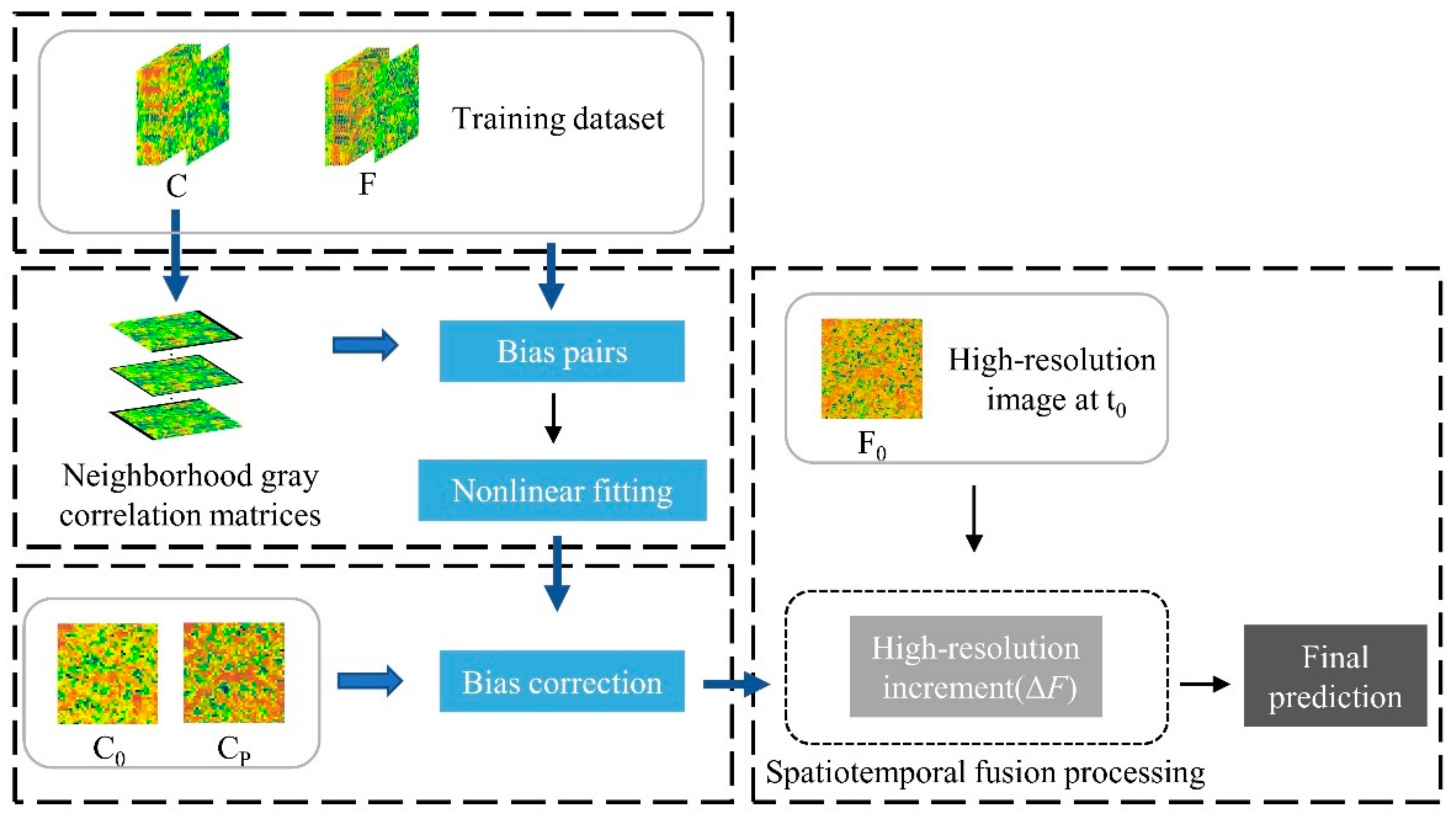
2. Methodology

The sensor-bias-based correction method consists of four steps: (1) generating neighborhood gray correlation matrices from low-spatial-resolution images; (2) establishing the bias pairs of different sensor images; (3) nonlinear fitting of image bias pairs using machine learning; and (4) correcting the low-spatial-resolution images. The corrected low-resolution images are then input into the spatiotemporal fusion algorithm to obtain the high-resolution increments, which are combined with the high-resolution image of the base date to generate the high-resolution image of the predicted date. The flowchart for this work is presented in Figure 1.

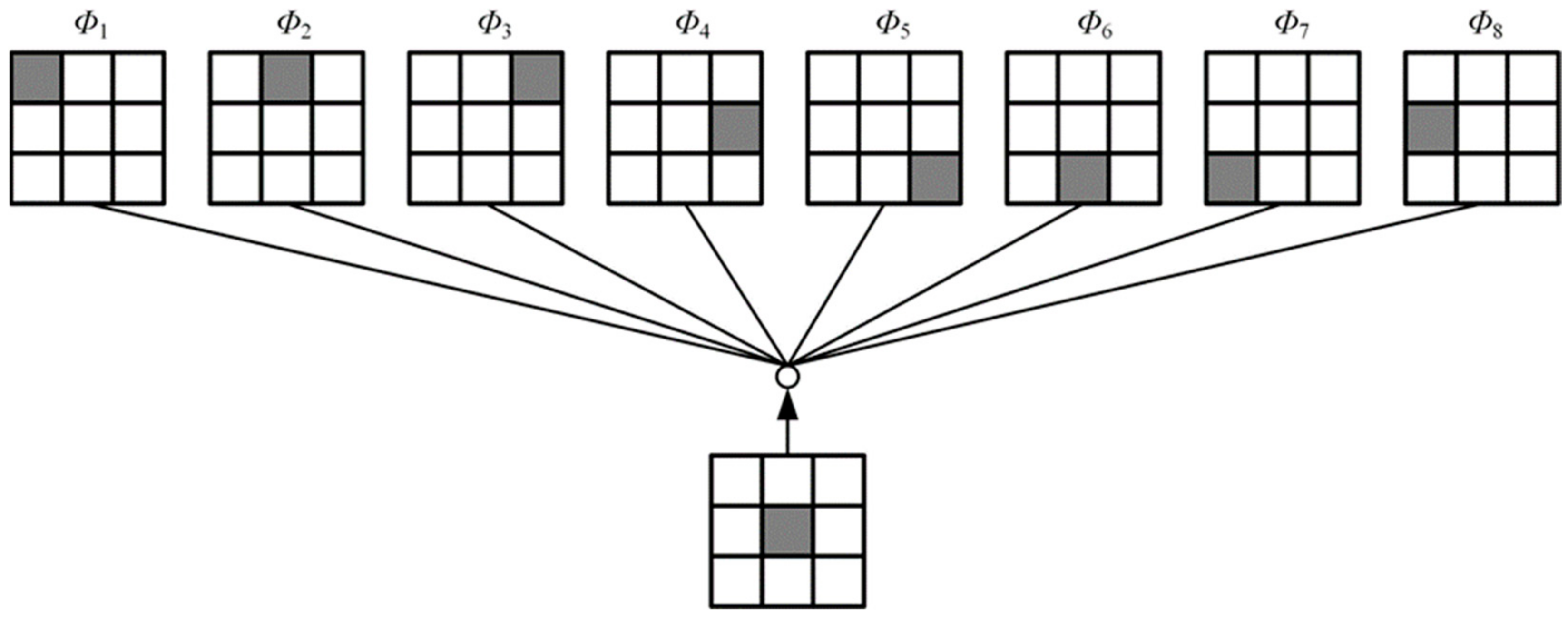
2.1. Generating Neighborhood Gray Correlation Matrices

Images with low and high spatial resolutions used as input data for spatiotemporal fusion models should be registered and calibrated to identical physical quantities. If the spatial resolution difference between the two observations is significant in the registration process, the low-resolution image is resampled to a high-resolution image using the nearest neighbor algorithm, one image is georeferenced to the other using control points, or the correlation between the two images is maximized, and then cropped to cover the identical area [31,47]. However, a big spatial resolution gap between the two types of observations causes registration errors.

Assuming that the resampled low-spatial-resolution image has a registration error of N pixels with the high-spatial-resolution image, N is usually set as a multiple of the scaling factor for the two types of sensors. The x-direction and y-direction are the column and row of the image, respectively. The reference pixels are denoted as ($x_i$, $y_j$), and the registration error is simulated to make the image pixels ($x_k$, $y_k$) with relative distance d equal to the value of reference pixels.

$$d_{ijk}=\sqrt{{\left(x_k-x_i\right)}^2+{\left(y_k-y_j\right)}^2 }$$

(1)

where $d_{ijk}$ represents the relative distance between the pixels with registration errors and the reference pixels, which is determined by N. A schematic diagram of the registration error direction (N = 1) is presented in Figure 2.

The neighborhood gray correlation matrix is generated by combining the registration errors and the neighboring pixels through a series of mathematical transformations. The resampled low-spatial-resolution image is used as the reference image. Padding N steps of 0 around the reference image shifts the matrix of the reference image by a set dimension in each direction. Each unique shift is stored as a new neighborhood correlation matrix, ensuring that each neighborhood pixel to be considered is in the same position as the reference pixel in the new neighborhood correlation matrix and the reference matrix, respectively. Finally, new neighborhood correlation matrices are compressed into a 3-dimensional matrix to generate the set of neighborhood correlation matrices. The registration error matrix $C_j^n$ is expressed as:

$$C_j^n=\Phi \left(C\left(x,y\right)+d_{ijk}\right)$$

(2)

where $C\left(x,y\right)$ indicates the reference matrix for images with low spatial resolution. Φ represents the registration error direction, determined by N, with a value of 8N.

The effects due to sensor differences are further characterized by using additional neighborhood information. When the registration error shift N ≥ 2 is assumed, considering the impacts of neighboring pixels at a relative distance m on the reference pixel, the neighbor pixel matrix $C_k^n$ is defined as:

$$C_k^n=\Phi \left(C\left(x,y\right)+d_{ijk}-m\right)$$

(3)

$$F^{\prime }\left(x,y,l\right)=\left[C,C_j^1,C_j^2,\cdots \cdots C_j^n,C_k^1,C_k^2,\cdots \cdots C_k^n\right]$$

(4)

where the range of m is (1…N − 1). $F^{\prime }\left(x,y,l\right)$ represents the set of neighborhood correlation matrices considering all possible registration errors and spatial neighborhood information, and $l$ represents the number of matrices as (2N + 1)².

2.2. Establishing Bias Pairs of Different Sensors

The difference between the two sensor observations $E_{FC}$ is expressed as:

$$E_{FC}=E_{BRDF}+E_{\mathrm{s}}+E_{\mathrm{t}}+E_{\mathrm{r}}$$

(5)

where FC represents the high-resolution image (e.g., Landsat) and low-resolution image (e.g., MODIS), $E_{BRDF}$ represents the difference generated by the bidirectional reflectance distribution function (BRDF) effect, $E_{\mathrm{s}}$ represents the systematic difference due to the difference in spectral band configuration between the two sensors, $E_{\mathrm{t}}$ represents the difference generated by the temporal intervals between observations, and $E_{\mathrm{r}}$ represents the difference in observations generated by the registration errors [46]. Therefore, the overall difference in the observations resulting from sensor bias, $E_{FC}$ is expressed as:

$$E_{FC}\left(x,y\right)=F\left(x,y\right)-C\left(x,y\right)$$

(6)

$$E_{F^{\prime }C}\left(x,y,l\right)=F^{\prime }\left(x,y,l\right)-C\left(x,y\right)$$

(7)

where $F\left(x,y\right)$ represents the matrix of the high-resolution image and $E_{F^{\prime }C}\left(x,y,l\right)$ denotes the bias of the neighborhood correlation matrix with the reference matrix.

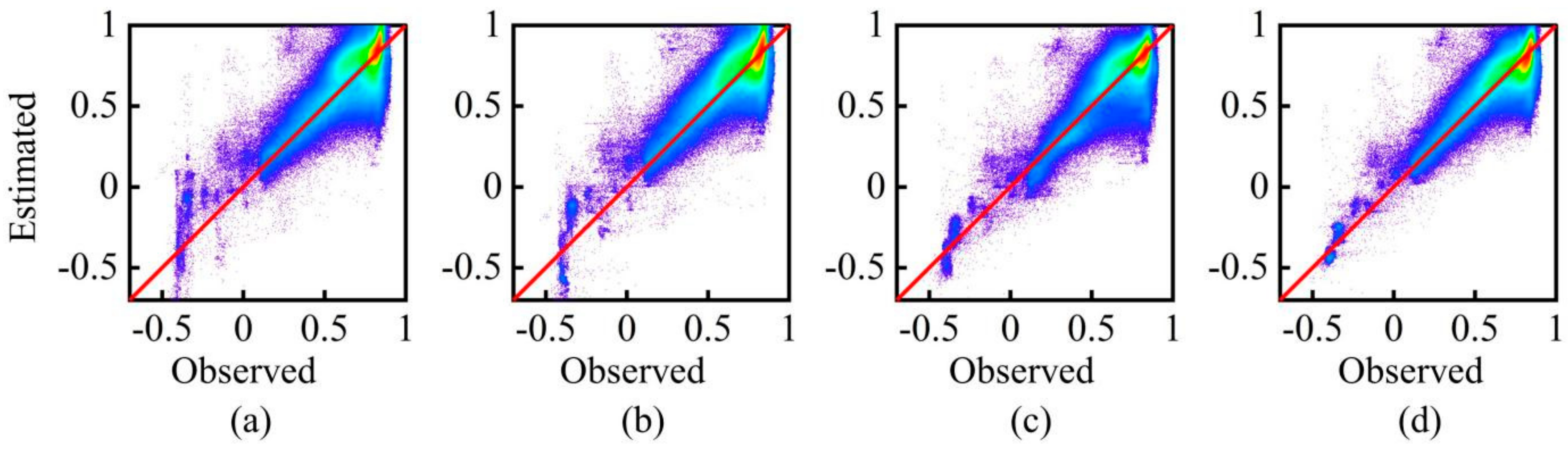
2.3. Nonlinear Fitting of Image Bias Pairs

After obtaining the bias pairs, a regression relationship needs to be established for each pair of bias pixels. The pixels in $E_{F^{\prime }C}\left(x,y,l\right)$ are treated as features that affect the generation of $E_{FC}\left(x,y\right)$. It is assumed that there is a registration error. When N’s value is larger, pixels farther away from the reference pixel may have a greater impact. However, in practice, we do not know the displacement and direction of the specific registration errors. Previously, empirical formulae were used to determine the weights of each feature. Although the calculation was simple and balanced the computational efficiency, it is not the most accurate solution.

The light gradient boosting machine (LGBM) [48] is widely used in the field of remote sensing, and research has proved that the LGBM has obvious advantages in computational speed and accuracy compared with other similar algorithms [49,50]. Given the advantages of machine learning in nonlinear mapping, we used the LGBM regression model to obtain the weights of each impact factor by nonlinearly fitting the bias pairs. In the model, a piecewise function is established for each feature value by a histogram optimization algorithm before training, thus, converting the feature values from continuous to discrete values. First, the information entropy of the training data $Ent\left(D\right)$ is calculated:

$$Ent\left(D\right)=-{{\displaystyle \sum }}_{i=1}^{Q}P\left(D^Q\right){log}_{2}P\left(D^Q\right)$$

(8)

where D represents the training dataset, $D^Q$ represents the discrete values of the optimized histogram of target sample features, and $P\left(D^Q\right)$ is the occurrence probability of each discrete value in D.

Second, assuming that a single feature $l_i$ has V discrete values after histogram optimization, if $l_i$ is used to partition the training dataset D, V subsets are generated, denoted as $D^v$. The information entropy of $D^v$ is calculated according to Equation (8). Considering that different subsets contain different numbers of samples, the subsets are given a weight $\frac{\left|D^v\right|}{\left|D\right|}$, i.e., more samples have a greater impact on the subset weights; therefore, information gain $Gain\left(D,l_i\right)$ obtained by dividing the sample set D using a single feature li can be calculated and expressed as follows.

$$Gain\left(D,l_i\right)=Ent\left(D\right)-{{\displaystyle \sum }}_{i=1}^V\frac{\left|D^v\right|}{\left|D\right|}Ent\left(D^v\right)$$

(9)

Thus, l information gain values are obtained, which are normalized to obtain the weight of each feature, denoted as $W_i$:

$$W_i=\frac{Gain\left(D,l_i\right)}{{{\displaystyle \sum }}_{i=1}^{l}Gain\left(D,l_i\right)}$$

(10)

Finally, the weighted sum of the different features is used to generate the sensor bias $E_{FC}\left(x,y\right)$:

$$E_{FC}\left(x,y\right)={{\displaystyle \sum }}_{i=1}^l{E}_{F^{\prime }C}\left(x,y,l\right)\ast W_i$$

(11)

2.4. Correcting the Low-Spatial-Resolution Images

The low-spatial-resolution image $C_t\left(x,y\right)$ to be corrected is taken as the reference matrix. The set $F_{C_t}^{\prime }\left(x,y,l\right)$ of neighboring gray correlation matrices of the reference matrix is generated by the equations in Section 2.1. Then the original image pixels are subtracted to obtain the deviation in the neighboring correlation matrix from the reference matrix and expressed as:

$$E_{F^{\prime }{C}_t}\left(x,y,l\right)=F_{C_t}^{\prime }\left(x,y,l\right)-C_t\left(x,y\right)$$

(12)

The predicted bias is added to the resampled low-resolution image $C_t\left(x,y\right)$ to obtain the corrected image:

$$C_c\left(x,y\right)=C_t\left(x,y\right)+{{\displaystyle \sum }}_{i=1}^l{E}_{F^{\prime }{C}_t}\left(x,y,l\right)\ast W_i$$

(13)

where $C_t$ and $C_c$ denote the low-resolution image before and after correction, respectively. Each pixel of the corrected low-resolution image considers all possible registration errors and neighborhood pixel information.

2.5. Predicting High-Resolution Image with Spatiotemporal Fusion Models

There are many different approaches to spatiotemporal fusion, but the main concept can be described as follows:

$$F_p=F_0+\Delta F$$

(14)

$$\Delta F=f\left(\Delta C\right)$$

(15)

The high-resolution increments ($\Delta F$) of the predicted known and predicted times are first estimated through the low-resolution increments ($\Delta C$) of the known and predicted times obtained by the spatiotemporal fusion model ($f$). Then, the predicted NDVI values for time t_p are obtained through the base high-resolution NDVI values ($F_0$) and the increments ($\Delta F$) [24]. In this research, using spatiotemporal fusion models, i.e., FSDAF and STARFM, the high-resolution increment ($\Delta F$) due to land cover change and intraclass variations were approximated by the changes in the corrected low-resolution images at different times. Then, they were summed with the high-resolution NDVI values at the base date (t₀) to obtain the predicted NDVI images ($F_p$).

3. Experiment

In this paper, we used Landsat and MODIS NDVI images derived from red-band reflectance and near-infrared-band reflectance as experimental data to analyze the effect of sensor bias correction strategies on spatiotemporal fusion methods. The experiments were carried out in three diverse geographical landscapes (Figure 3), and two spatiotemporal fusion methods, FSDAF and STARFM, were utilized.

3.1. Experimental Area and Data

The first experimental area is located in the Coleambally Irrigation Area, Australia (34°54′S, 145°57′E), a region with highly varied terrain characterized by many small patchy fields and fast phenological variations. Two Landsat ETM+ images (800 × 800 pixels, with a resampling resolution of 25 m) obtained on December 04, 2001 (t₀) and 12 January 2002 (t_p), and corresponding daily MODIS images (MOD09GA Collection 5) were chosen as experimental data (Figure 4).

The second study site is located in the Gwydir area, Australia (149.2818°E, 29.0855°S). Two Landsat 5 TM images (800 × 800 pixels, with a resampling resolution of 25 m) were obtained on 26 November 2004 (t₀) and 12 December 2004 (t_p), and MOD09GA images obtained on the same dates were utilized (Figure 5). The test images of the above two sites were obtained from the open-source spatiotemporal fusion experimental dataset [31].

The third experimental site in western Jilin Province, China (44°40′–44°56′N and 123°44′–124°7′E), covering an area of 29 km × 29 km (960 × 960 Landsat image pixels), is a homogeneous landscape where the main land cover type is farmland, water bodies, and construction land (Figure 6). At present, sensors, such as Landsat 5 TM, have been discontinued. Furthermore, the use of images on neighboring dates will increase $E_{\mathrm{t}}$ in Equation (5), which will increase the uncertainty in the spatiotemporal fusion results. Therefore, the analysis of the influence of the bias correction method on the fusion results with date-adjacent images demonstrates the potential of the proposed method to generate high-resolution images of long time series. We selected two Landsat8 OLI images acquired on 1 July 2018 (t₀) and 2 August 2018 (t_p), and the corresponding adjacent MOD09A1 images acquired on 26 June 2018 and 28 July 2018, as experimental data, and resampled the spatial resolution of the MOD09A1 images to 30 m to match the Landsat image.

3.2. Experimental Design and Evaluation

Our experiments used 11 pairs of preprocessed Landsat and MODIS images from adjacent dates (t₀ and t_p) for the above three sites as training data. As MODIS images in the open-source dataset have been preprocessed with nearest neighbor resampling, we employed it as the default resampling method for the consistency of the experiments. For the correction and fusion process, the registration shift N and the scaling factor of the spatiotemporal fusion model were assumed to be 20 in the Coleambally and Gwydir areas, and the two parameters for the western Jilin area were set to 16. The rest of the parameters used the default values.

As the STARFM is a spatiotemporal fusion model designed for fixed sensor pairs, we employed a version of the STARFM that can be used for diverse sensors to verify the correctness of the results [22]. We compared the fusion results of the STARFM and FSDAF model through visual assessment and quantitative measurements, in which input was processed by sensor bias correction and nearest-neighbor resampling, respectively. The predicted date’s high-resolution images (Landsat NDVI) were regarded as actual data. The predicted Landsat-like images were quantitatively compared to the actual Landsat images. The root mean square error (RMSE) and correlation coefficient (CC) were used to measure the difference and the degree of relevance between the fused NDVI image and the real NDVI image. A smaller RMSE means a better prediction. The average difference (AD) between two NDVI images can reflect the overall deviation in the prediction. Generally, a positive AD value means that the fused NDVI image overestimates the actual values, whereas a negative AD means an underestimate. Structural similarity (SSIM) is a metric used to assess the structural similarity of real and fused NDVI images. High similarity between two images exists when the RMSE (or AD) value is close to 0 or the CC (or SSIM) value is close to 1.

4. Results

4.1. Fusion of the NDVI after Sensor Bias Correction in Heterogeneous Landscape Areas

The experimental area has a high spatial heterogeneity and no significant land cover changes, but the crop phenology changes rapidly between the two time periods. Figure 7 shows a visual comparison of the Landsat NDVI images predicted by FSDAF and the STARFM before and after the bias correction process for the Landsat NDVI image (actual image) observed on 12 January 2002. The STARFM-predicted NDVI image without bias correction captured most seasonal changes but generated patches with uniform values (Figure 7b). In the FSDAF-predicted image, phenological information was predicted, but more discontinuity existed in the areas of rapid phenological changes (Figure 7e). In contrast, after bias correction, errors (e.g., the speckle noise) in the regions with phenological changes in the NDVI images predicted by FSDAF were significantly reduced (Figure 7c). The NDVI of plant covers in the real image is dark blue (Figure 7d). The fusion result of the STARFM after correction removed the patches and is also visually similar to the actual NDVI image (Figure 7f). Figure 8 and

Table 1. Accuracy of the STARFM- and FSDAF-predicted NDVIs before and after bias correction of input data for the Coleambally Irrigation Area. Best results are marked in bold.

Methods	Image	CC	RMSE	AD	SSIM
FSDAF	uncorrected	0.7974	0.1563	−0.0072	0.6837
	corrected	0.8269	0.1449	0.0002	0.6901
STARFM	uncorrected	0.7990	0.1577	−0.0133	0.6976
	corrected	0.8406	0.1416	−0.0056	0.7186

show that the NDVIs predicted by FSDAF and the STARFM after bias correction were more accurate and closer to the 1:1 line than the precorrection results.

For the whole image, the fusion results of FSDAF obtained after correction were highly correlated with the actual NDVI (CC = 0.8269 and RMSE = 0.1449). The increases in structural similarity (SSIM) reduced the blur caused by pixel discontinuities. For the STARFM, the bias-corrected inputs of the fusion results showed a higher CC (0.8406), lower RMSE (0.1416), and higher SSIM (0.7186). Compared to the actual Landsat NDVI, the low AD values were 0.0002 and −0.0056, indicating the high accuracy of NDVI fusion by FSDAF and the STARFM after bias correction.

4.2. Fusion of NDVI Images after Sensor Bias Correction in Areas of Dramatic Land Cover Change

By visual comparison, the bias-uncorrected FSDAF- and STARFM-predicted NDVI images captured partial land cover change information at the Gwydir site (Figure 9). The predicted images included large-area flood inundation; however, such extensive flooding areas were not found in the actual Landsat NDVI images. In the areas of land cover change, the image generated by FSDAF after the correction process (RMSE = 0.1315) still had speckle noise compared to the predicted image without bias correction (Figure 9b). More land cover changes could be captured and generate the boundary of flooding in the real image (Figure 9c). The NDVI image (RMSE = 0.1204) predicted by the STARFM after bias correction had many fuzzy spatial details but was more similar to the actual NDVI image (Figure 9a) than the predicted image before correction (Figure 9d), therefore, reducing the misjudgment of pixels of unchanged land cover and false flooded areas (circle area marked in Figure 9).

As the CC and AD values are shown in

Table 2. Accuracy of the STARFM- and FSDAF-predicted NDVIs before and after bias correction of input data for the Gwydir area. Best results are marked in bold.

Methods	Image	CC	RMSE	AD	SSIM
FSDAF	uncorrected	0.7586	0.1507	−0.0448	0.4561
	corrected	0.7960	0.1315	−0.0013	0.5027
STARFM	uncorrected	0.7817	0.1432	-0.0458	0.5006
	corrected	0.8316	0.1204	−0.0013	0.5556

, after the correction process, both the NDVI fusion images predicted by the two models were highly correlated to the actual NDVI image with almost no deviation. The spatiotemporal fusion model’s robustness and accuracy in predicting images of areas with changing land cover improved. SSIM found that bias-corrected fusion images retrieved changed features and retained spatial details better than bias-uncorrected fusion images. As illustrated in Figure 10, the scatter points of the bias-corrected fusion NDVI results obtained using FSDAF and the STARFM were more concentrated and were closer to the 1:1 line than those of the bias-uncorrected fusion results.

4.3. NDVI Fusion after Sensor Bias Correction in Homogeneous Regions

Figure 11 shows the predicted Landsat-like NDVI before and after bias correction and the Landsat NDVI observed on the predicted dates for the homogeneous landscape region of western Jilin, China. With the MODIS and Landsat images of the adjacent dates, the fusion NDVI predicted by the original FSDAF algorithm based on the uncorrected input data generated obvious errors in some pixels, e.g., the blocky artifacts (Figure 11b, area within the dashed circle). The images predicted by the STARFM lost many spatial details and were visually blurred due to over-smoothing (Figure 11e). In contrast, the NDVI image predicted by FSDAF after the input data performed bias correction showed more spatial details, and blocky artifacts were eliminated (Figure 11c). The blurring effects in the fused image obtained by the STARFM were somewhat alleviated, generating spatial details that were more similar to those of the actual Landsat NDVI image of the predicted date (Figure 11f).

Table 3. Accuracy of STARFM- and FSDAF-predicted NDVI images before and after bias correction of input data in an area of western Jilin, China. Best results are marked in bold.

Methods	Image	CC	RMSE	AD	SSIM
FSDAF	uncorrected	0.8525	0.1149	0.0220	0.6257
	corrected	0.8742	0.1055	0.0003	0.6538
STARFM	uncorrected	0.8693	0.1066	0.0207	0.6582
	corrected	0.8869	0.0967	−0.0016	0.6684

shows the accuracy of the fusion results obtained using spatiotemporal models before and after bias correction of input data for an area in west Jilin, China. Compared to the bias-uncorrected FSDAF and STARFM predictions, the fused NDVI image after correction had a lower RMSE, a higher CC, and higher SSIM values relative to the actual NDVI data, indicating that the spatiotemporal fusion algorithms after bias correction of input data might be better at retrieving the spectral and structural information of images. Moreover, according to the AD value, the fusion result had almost no deviation from the actual NDVI, suggesting improved robustness of the spatiotemporal fusion model. From Figure 12, the NDVI values predicted by the spatiotemporal fusion method after bias correction showed less dispersion and were more similar to the actual NDVI values, which indicates that the bias correction method might reduce the uncertainty caused by the original spatiotemporal fusion algorithm when using images from adjacent dates.

5. Discussion

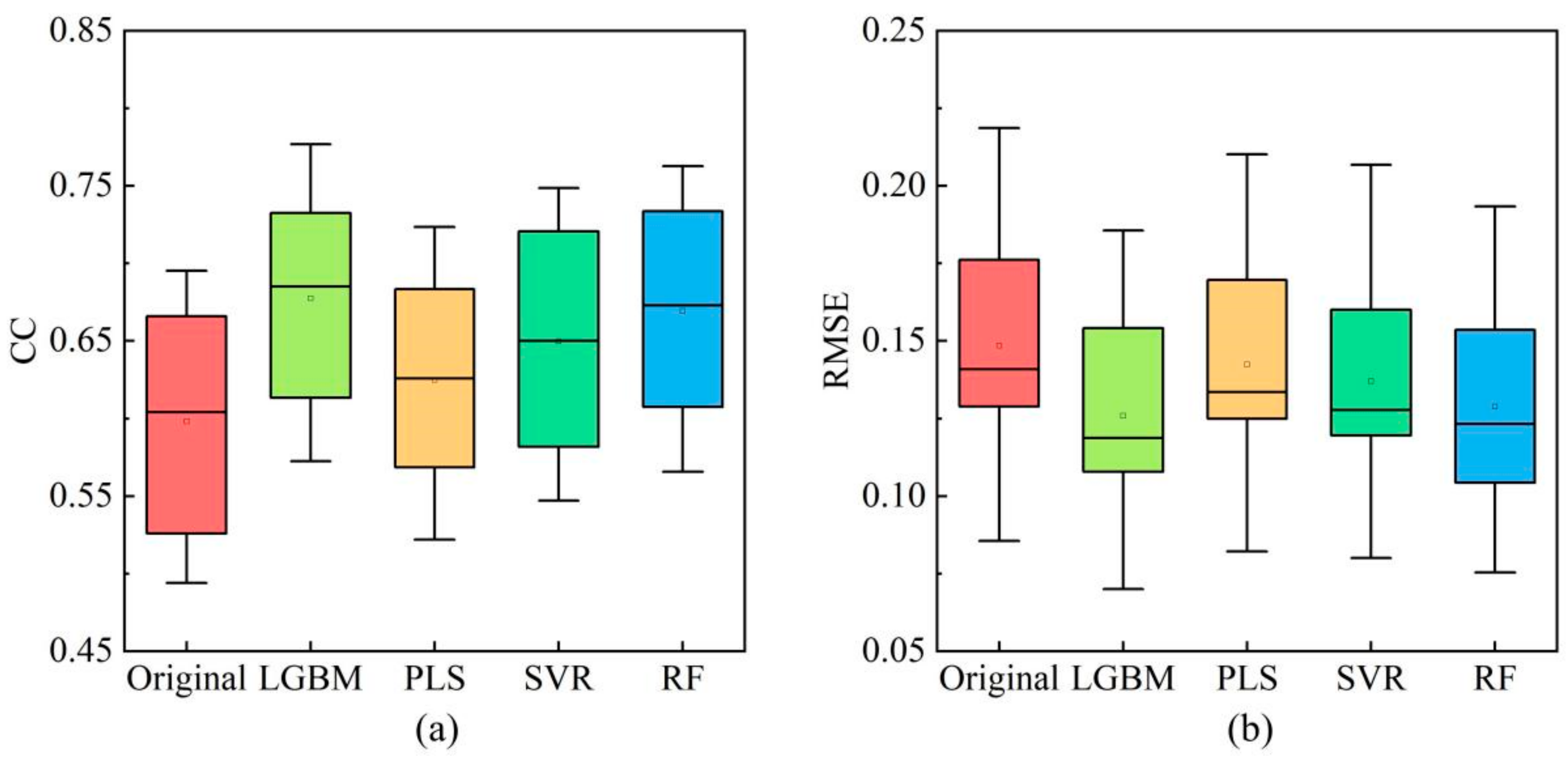
5.1. Effect of Different Regression Algorithms on Correction Models

Different regression methods may have different effects on the model of sensor bias correction. Here, we selected four popular regression methods, namely, the random forest (RF) regression method [51], the support vector regression (SVR) method [52], the partial least squares regression (PLS) method [53], and the light gradient boosting machine (LGBM) regression method [48], to analyze their influences on the bias correction method. The MODIS NDVI of the three experimental areas was divided into three sets of test data. To evaluate the effects of the four regression methods, they were evaluated based on the correlation coefficient (CC) and root mean square difference (RMSE) between the test data (before and after correction) and the corresponding Landsat NDVI.

Figure 13 illustrates that the bias correction method driven by the four regression methods performed well in terms of CC and RMSE. In the three test datasets, the LGBM algorithm showed more consistent performance in correcting sensor bias compared to the RF, SVR, and PLS algorithms with minimum average RMSEs of 0.1258 (Table S1) and maximum average CCs of 0.7768 (Table S2). The average RMSEs decreased by 15.29% and the average CCs increased by 13.25% compared to the pre-correction. The corrected MODIS NDVI deviated the least from the corresponding Landsat NDVI after correction by using the LGBM-driven bias correction method (Figure 13). Figure 14 shows the spatial distribution of the absolute difference between MODIS NDVI and the corresponding Landsat NDVI before and after correction with the LGBM-driven bias correction method. The enlarged images are used for better visual comparison. The lighter color in Figure 14 represents the smaller absolute difference. It can be seen that the corrected MODIS NDVI is closer to the actual Landsat NDVI, which proves the effectiveness of the correction method. On the whole, the LGBM algorithm is the most suitable for sensor bias correction among the four regression algorithms in terms of performance index and visual results.

5.2. Effect of Bias Correction on the Input Image for Spatiotemporal Fusion

The differences between sensors may result in inconsistent phenological changes and land cover changes expressed by different sensors at the predicted time [54]. As seen in Equation (15), the estimation of the high-resolution increment (ΔF) depends on the incremental change (ΔC) in the low-resolution image between different times. Due to the absence of a high-resolution image on the prediction date, all relevant information on land cover type change and intraclass variability are included in the low-resolution image.

In this study, we found that in the heterogeneous landscape region with rapid phenological changes, compared to the nearest neighbor resampled increment ΔC (Figure 15b), the bias-corrected increment ΔC (Figure 15c) had a higher correlation with the actual high-resolution NDVI increment ΔF (Figure 15a), with a higher correlation coefficient (CC = 0.6214) and a smaller RMSE (0.1473). In the area of intense changes in land cover, compared with the increment acquired from resampling (Figure 15e), the increment obtained after bias correction (Figure 15f) determined more accurate change information and was closer to the actual high-resolution increment ΔF (Figure 15d). In the western region of Jilin, due to the large observation date interval of the high- and low-resolution image pairs at t₀, the NDVI increment of MODIS at different times (Figure 15h) differed greatly from the true high-resolution NDVI increment (Figure 15g). In contrast, the corrected ΔC (Figure 15i) was more closely correlated with the high-resolution increment ΔF (CC = 0.6214). The proposed bias correction method can effectively reduce the uncertainty of the input data increment (ΔC) caused by rapid changes in the phenological period, drastic changes in land cover, and large date intervals between sensors. Correcting the low-resolution input image to generate reliable spatial distributions provides a strong guarantee for obtaining a more accurate high-resolution increment (ΔF) of temporal prediction.

5.3. Effect of Bias Correction on the Spatiotemporal Fusion Results

Equation (14) shows that the spatiotemporal fusion result depends on the accuracy of the increment ΔF estimation. In three experiments for different landscapes, the accuracies of the predicted NDVI from the two bias-corrected spatiotemporal models were both improved. By comparing the four indexes (i.e., RMSE, CC, AD, and SSIM), we found that the improvement in fusion accuracy by the STARFM after bias correction was better than that by bias-corrected FSDAF.

FSDAF is regarded as a hybrid spatiotemporal fusion model that combines the unmixing method, spatial interpolation, and weight function into one framework [20,26]. In the process of FSDAF, the high-resolution increment ΔF is estimated by using land cover type change information obtained from the unmixing method, the distribution of residuals guided by thin plate spline (TPS) interpolation, and the information of weighted neighborhood changes. FSDAF works well for land cover change visible in the low-resolution image. In this study, the value changes for most bias-corrected image pixels have small effects on the results when estimating the temporal changes of each land cover type in coarse images, indicating that FSDAF has excellent robustness. In contrast, the STARFM estimates high-resolution pixel values by combining information from all input images through weight functions. It utilizes the change information of the neighboring similar image pixels (i.e., spatial proximity, spectral similarity, and change similarity) to predict the target pixel. One of the key steps in the STARFM is to find the pixels with spectral features similar to those of the reference image pixels. In Figure 15, the changes in pixel values in the corrected low-resolution images are more similar to the real value variations. The bias correction helps to find similar pixels and obtain weights more accurately; thus, the accuracy of STARFM prediction may greatly improve.

5.4. Applicability of the Bias Correction Method

The correction method based on sensor bias is suitable for spatiotemporal fusion models that require the same spatial resolution of the input data (e.g., STARFM and FSDAF), which is not applicable to spatiotemporal fusion models with different requirements for the input data (e.g., Fit-FC and SFSDAF). It requires learning the biases between high- and low-spatial-resolution images of the same region to establish a mathematical model characterizing the nonlinear relationship between sensor biases. In this paper, the effectiveness of the correction method is demonstrated by testing on areas with different landscapes, especially in areas with rapid land cover changes. For regions with high heterogeneity with rapid land cover changes, the correction reduced the misjudgment of drastically changing pixels during spatiotemporal fusion prediction and enhanced blurred spatial details. However, errors, such as speckle noise, could not be completely eliminated due to the limitations in the spatiotemporal fusion model.

6. Conclusions

We propose a simple and effective correction method to quantify sensor bias to address the uncertainty of spatiotemporal fusion results due to sensor differences and pre-processing. Using the correction method, the contrast information of low-spatial-resolution images can effectively be recovered, and a higher correlation with high-spatial-resolution images with land cover type changes can be maintained. After bias correction, the correlation between high- and low-spatial-resolution images of neighboring dates increases, thus, extending the available date range of input images in the spatiotemporal fusion algorithm. The accuracy of the fusion results improved for different landscape feature areas, especially in areas with drastic land cover changes. The findings are summarized as follows.

(1)

The machine learning algorithm is introduced to quantify sensor bias, which mitigates the uncertain effects of sensor differences and preprocessing on fusion results and provides optimized input data for spatiotemporal fusion.

(2)

Sensor bias correction helps to improve the robustness and usability of spatiotemporal fusion algorithms in different types of landscapes.

(3)

The bias correction method reduces the misjudgment of pixels and occurrence of blocky or blurring effects induced by the spatiotemporal fusion model in areas with high heterogeneity or drastic land cover changes, thus, effectively recovering the changed features and retaining more spatial details.

(4)

By bias correction, the availability of high- and low-spatial-resolution image pairs for adjacent dates without large-scale land cover changes will be improved, providing convenience for generating large-scale high-spatiotemporal-resolution datasets through spatiotemporal fusion models.

References

- Gao, F.; Masek, J.; Schwaller, M.; Hall, F. On the blending of the Landsat and MODIS surface reflectance: Predicting daily Landsat surface reflectance. IEEE Trans. Geosci. Remote Sens. 2006, 44, 2207–2218. [Google Scholar] [CrossRef]
- Huang, B.; Wang, J.; Song, H.; Fu, D.; Wong, K. Generating high spatiotemporal resolution land surface temperature for urban heat island monitoring. IEEE Geosci. Remote Sens. Lett. 2013, 10, 1011–1015. [Google Scholar] [CrossRef]
- Wang, J.; Schmitz, O.; Lu, M.; Karssenberg, D. Thermal unmixing based downscaling for fine resolution diurnal land surface temperature analysis. ISPRS J. Photogramm. Remote Sens. 2020, 161, 76–89. [Google Scholar] [CrossRef]
- Weng, Q.; Fu, P.; Gao, F. Generating daily land surface temperature at Landsat resolution by fusing Landsat and MODIS data. Remote Sens. Environ. 2014, 145, 55–67. [Google Scholar] [CrossRef]
- Meng, J.; Du, X.; Wu, B. Generation of high spatial and temporal resolution NDVI and its application in crop biomass estimation. Int. J. Digit. Earth 2013, 6, 203–218. [Google Scholar] [CrossRef]
- Tewes, A.; Thonfeld, F.; Schmidt, M.; Oomen, R.J.; Zhu, X.; Dubovyk, O.; Menz, G.; Schellberg, J. Using RapidEye and MODIS data fusion to monitor vegetation dynamics in semi-arid rangelands in South Africa. Remote Sens. 2015, 7, 6510–6534. [Google Scholar] [CrossRef] [Green Version]
- Chen, B.; Chen, L.; Huang, B.; Michishita, R.; Xu, B. Dynamic monitoring of the Poyang Lake wetland by integrating Landsat and MODIS observations. ISPRS J. Photogramm. Remote Sens. 2018, 139, 75–87. [Google Scholar] [CrossRef]
- Ke, Y.; Im, J.; Park, S.; Gong, H. Spatiotemporal downscaling approaches for monitoring 8-day 30 m actual evapotranspiration. ISPRS J. Photogramm. Remote Sens. 2017, 126, 79–93. [Google Scholar] [CrossRef]
- Ke, Y.; Im, J.; Park, S.; Gong, H. Downscaling of MODIS One kilometer evapotranspiration using Landsat-8 data and machine learning approaches. Remote Sens. 2016, 8, 215. [Google Scholar] [CrossRef] [Green Version]
- Houborg, R.; McCabe, M.F.; Gao, F. A spatio-temporal enhancement method for medium resolution LAI (STEM-LAI). Int. J. Appl. Earth Obs. Geoinf. 2016, 47, 15–29. [Google Scholar] [CrossRef] [Green Version]
- Zhai, H.; Huang, F.; Qi, H. Generating high resolution LAI based on a modified FSDAF model. Remote Sens. 2020, 12, 150. [Google Scholar] [CrossRef] [Green Version]
- Zhang, H.; Chen, J.M.; Huang, B.; Song, H.; Li, Y. Reconstructing seasonal variation of Landsat vegetation index related to leaf area index by fusing with MODIS data. IEEE J. Sel. Top. Appl. Earth Obs. Remote Sens. 2014, 7, 950–960. [Google Scholar] [CrossRef]
- Busetto, L.; Meroni, M.; Colombo, R. Combining medium and coarse spatial resolution satellite data to improve the estimation of sub-pixel NDVI time series. Remote Sens. Environ. 2008, 112, 118–131. [Google Scholar] [CrossRef]
- Xu, Y.; Huang, B.; Xu, Y.; Cao, K.; Guo, C.; Meng, D. Spatial and temporal image fusion via regularized spatial unmixing. IEEE Geosci. Remote Sens. Lett. 2015, 12, 1362–1366. [Google Scholar] [CrossRef]
- Zhukov, B.; Oertel, D.; Lanzl, F.; Reinhäckel, G. Unmixing-based multisensor multiresolution image fusion. IEEE Trans. Geosci. Remote Sens. 1999, 37, 1212–1226. [Google Scholar] [CrossRef]
- Jamshidi, S.; Zand-Parsa, S.; Jahromi, M.N.; Niyogi, D. Application of a simple Landsat-MODIS fusion model to estimate evapotranspiration over a heterogeneous sparse vegetation region. Remote Sens. 2019, 11, 741. [Google Scholar] [CrossRef] [Green Version]
- Zhu, X.; Helmer, E.H.; Gao, F.; Liu, D.; Chen, J.; Lefsky, M.A. A flexible spatiotemporal method for fusing satellite images with different resolutions. Remote Sens. Environ. 2016, 172, 165–177. [Google Scholar] [CrossRef]
- Huang, B.; Song, H. Spatiotemporal reflectance fusion via sparse representation. IEEE Trans. Geosci. Remote Sens. 2012, 50, 3707–3716. [Google Scholar] [CrossRef]
- Song, H.; Liu, Q.; Wang, G.; Hang, R.; Huang, B. Spatiotemporal satellite image fusion using deep convolutional neural networks. IEEE J. Sel. Top. Appl. Earth Obs. Remote Sens. 2018, 11, 821–829. [Google Scholar] [CrossRef]
- Zhu, X.; Cai, F.; Tian, J.; Williams, T.K.A. Spatiotemporal fusion of multisource remote sensing data: Literature survey, taxonomy, principles, applications, and future directions. Remote Sens. 2018, 10, 527. [Google Scholar] [CrossRef] [Green Version]
- Luo, Y.; Guan, K.; Peng, J. STAIR: A generic and fully-automated method to fuse multiple sources of optical satellite data to generate a high-resolution, daily and cloud-/gap-free surface reflectance product. Remote Sens. Environ. 2018, 214, 87–99. [Google Scholar] [CrossRef]
- Mileva, N.; Mecklenburg, S.; Gascon, F. New tool for spatio-temporal image fusion in remote sensing: A case study approach using Sentinel-2 and Sentinel-3 data. In Image and Signal Processing for Remote Sensing XXIV; SPIE: Bellingham, DC, USA, 2018; p. 20. [Google Scholar]
- Zhu, X.; Chen, J.; Gao, F.; Chen, X.; Masek, J.G. An enhanced spatial and temporal adaptive reflectance fusion model for complex heterogeneous regions. Remote Sens. Environ. 2010, 114, 2610–2623. [Google Scholar] [CrossRef]
- Liu, M.; Yang, W.; Zhu, X.; Chen, J.; Chen, X.; Yang, L.; Helmer, E.H. An Improved Flexible Spatiotemporal DAta Fusion (IFSDAF) method for producing high spatiotemporal resolution normalized difference vegetation index time series. Remote Sens. Environ. 2019, 227, 74–89. [Google Scholar] [CrossRef]
- Li, X.; Foody, G.M.; Boyd, D.S.; Ge, Y.; Zhang, Y.; Du, Y.; Ling, F. SFSDAF: An enhanced FSDAF that incorporates sub-pixel class fraction change information for spatio-temporal image fusion. Remote Sens. Environ. 2020, 237, 111537. [Google Scholar] [CrossRef]
- Guo, D.; Shi, W.; Hao, M.; Zhu, X. FSDAF 2.0: Improving the performance of retrieving land cover changes and preserving spatial details. Remote Sens. Environ. 2020, 248, 111973. [Google Scholar] [CrossRef]
- Zheng, Y.; Song, H.; Sun, L.; Wu, Z.; Jeon, B. Spatiotemporal fusion of satellite images via very deep convolutional networks. Remote Sens. 2019, 11, 2701. [Google Scholar] [CrossRef] [Green Version]
- Zhang, H.; Song, Y.; Han, C.; Zhang, L. Remote Sensing Image Spatiotemporal Fusion Using a Generative Adversarial Network. IEEE Trans. Geosci. Remote Sens. 2021, 59, 4273–4286. [Google Scholar] [CrossRef]
- Tan, Z.; Yue, P.; Di, L.; Tang, J. Deriving high spatiotemporal remote sensing images using deep convolutional network. Remote Sens. 2018, 10, 1066. [Google Scholar] [CrossRef] [Green Version]
- Jia, D.; Cheng, C.; Shen, S.; Ning, L. Multitask Deep Learning Framework for Spatiotemporal Fusion of NDVI. IEEE Trans. Geosci. Remote Sens. 2022, 60, 5616313. [Google Scholar] [CrossRef]
- Emelyanova, I.V.; McVicar, T.R.; Van Niel, T.G.; Li, L.T.; van Dijk, A.I.J.M. Assessing the accuracy of blending Landsat-MODIS surface reflectances in two landscapes with contrasting spatial and temporal dynamics: A framework for algorithm selection. Remote Sens. Environ. 2013, 133, 193–209. [Google Scholar] [CrossRef]
- Wang, Q.; Atkinson, P.M. Spatio-temporal fusion for daily Sentinel-2 images. Remote Sens. Environ. 2018, 204, 31–42. [Google Scholar] [CrossRef] [Green Version]
- Liu, M.; Ke, Y.; Yin, Q.; Chen, X.; Im, J. Comparison of five spatio-temporal satellite image fusion models over landscapes with various spatial heterogeneity and temporal variation. Remote Sens. 2019, 11, 2612. [Google Scholar] [CrossRef] [Green Version]
- Zhou, J.; Chen, J.; Chen, X.; Zhu, X.; Qiu, Y.; Song, H.; Rao, Y.; Zhang, C.; Cao, X.; Cui, X. Sensitivity of six typical spatiotemporal fusion methods to different influential factors: A comparative study for a normalized difference vegetation index time series reconstruction. Remote Sens. Environ. 2021, 252, 112130. [Google Scholar] [CrossRef]
- Privette, J.L.; Fowler, C.; Wick, G.A.; Baldwin, D.; Emery, W.J. Effects of orbital drift on advanced very high resolution radiometer products: Normalized difference vegetation index and sea surface temperature. Remote Sens. Environ. 1995, 53, 164–171. [Google Scholar] [CrossRef]
- Teillet, P.M.; Staenz, K.; Williams, D.J. Effects of spectral, spatial, and radiometric characteristics on remote sensing vegetation indices of forested regions. Remote Sens. Environ. 1997, 61, 139–149. [Google Scholar] [CrossRef]
- Teillet, P.M.; Fedosejevs, G.; Thome, K.J.; Barker, J.L. Impacts of spectral band difference effects on radiometric cross-calibration between satellite sensors in the solar-reflective spectral domain. Remote Sens. Environ. 2007, 110, 393–409. [Google Scholar] [CrossRef]
- Fan, X.; Liu, Y. Multisensor Normalized Difference Vegetation Index Intercalibration: A Comprehensive Overview of the Causes of and Solutions for Multisensor Differences. IEEE Geosci. Remote Sens. Mag. 2018, 6, 23–45. [Google Scholar] [CrossRef]
- Brown, M.E.; Pinzón, J.E.; Didan, K.; Morisette, J.T.; Tucker, C.J. Evaluation of the consistency of Long-term NDVI time series derived from AVHRR, SPOT-vegetation, SeaWiFS, MODIS, and Landsat ETM+ sensors. IEEE Trans. Geosci. Remote Sens. 2006, 44, 1787–1793. [Google Scholar] [CrossRef]
- Liang, S.; Strahler, A.H.; Barnsley, M.J.; Borel, C.C.; Gerstl, S.A.W.; Diner, D.J.; Prata, A.J.; Walthall, C.L. Multiangle remote sensing: Past, present and future. Remote Sens. Rev. 2000, 18, 83–102. [Google Scholar] [CrossRef]
- Obata, K.; Taniguchi, K.; Matsuoka, M.; Yoshioka, H. Development and Demonstration of a Method for Geo-to-Leo NDVI Transformation. Remote Sens. 2021, 13, 4085. [Google Scholar] [CrossRef]
- Latifovic, R.; Cihlar, J.; Chen, J. A comparison of BRDF models for the normalization of sallite optical data to a standard sun-target-sensor geometry. IEEE Trans. Geosci. Remote Sens. 2003, 41, 1889–1898. [Google Scholar] [CrossRef]
- Franke, J.; Heinzel, V.; Menz, G. Assessment of NDVI- Differences caused by sensor-specific relative spectral response functions. In Proceedings of the International Geoscience and Remote Sensing Symposium (IGARSS), Denver, CO, USA, 31 July 2006–4 August 2006; pp. 1130–1133. [Google Scholar]
- Trishchenko, A.P.; Cihlar, J.; Li, Z. Effects of spectral response function on surface reflectance and NDVI measured with moderate resolution satellite sensors. Remote Sens. Environ. 2002, 81, 1–18. [Google Scholar] [CrossRef]
- Wang, J.; Huang, B. A rigorously-weighted spatiotemporal fusion model with uncertainty analysis. Remote Sens. 2017, 9, 990. [Google Scholar] [CrossRef] [Green Version]
- Shi, W.; Guo, D.; Zhang, H. A reliable and adaptive spatiotemporal data fusion method for blending multi-spatiotemporal-resolution satellite images. Remote Sens. Environ. 2022, 268, 112770. [Google Scholar] [CrossRef]
- Gevaert, C.M.; García-Haro, F.J. A comparison of STARFM and an unmixing-based algorithm for Landsat and MODIS data fusion. Remote Sens. Environ. 2015, 156, 34–44. [Google Scholar] [CrossRef]
- Ke, G.; Meng, Q.; Finley, T.; Wang, T.; Chen, W.; Ma, W.; Ye, Q.; Liu, T.Y. LightGBM: A highly efficient gradient boosting decision tree. Adv. Neural Inf. Processing Syst. 2017, 30, 3147–3155. [Google Scholar]
- Sun, X.; Guo, L.; Zhang, W.; Wang, Z.; Yu, Q. Small Aerial Target Detection for Airborne Infrared Detection Systems Using LightGBM and Trajectory Constraints. IEEE J. Sel. Top. Appl. Earth Obs. Remote Sens. 2021, 14, 9959–9973. [Google Scholar] [CrossRef]
- Cao, J.; Zhang, Z.; Tao, F.; Zhang, L.; Luo, Y.; Han, J.; Li, Z. Identifying the contributions of multi-source data for winter wheat yield prediction in China. Remote Sens. 2020, 12, 750. [Google Scholar] [CrossRef] [Green Version]
- Breiman, L. Random forests. Mach. Learn. 2001, 45, 5–32. [Google Scholar] [CrossRef] [Green Version]
- Tuia, D.; Verrelst, J.; Alonso, L.; Perez-Cruz, F.; Camps-Valls, G. Multioutput support vector regression for remote sensing biophysical parameter estimation. IEEE Geosci. Remote Sens. Lett. 2011, 8, 804–808. [Google Scholar] [CrossRef]
- Geladi, P.; Kowalski, B.R. Partial least-squares regression: A tutorial. Anal. Chim. Acta 1986, 185, 1–17. [Google Scholar] [CrossRef]
- Shi, C.; Wang, X.; Zhang, M.; Liang, X.; Niu, L.; Han, H.; Zhu, X. A comprehensive and automated fusion method: The enhanced flexible spatiotemporal data fusion model for monitoring dynamic changes of land surface. Appl. Sci. 2019, 9, 3693. [Google Scholar] [CrossRef] [Green Version]