Middle- and Long-Term UT1-UTC Prediction Based on Constrained Polynomial Curve Fitting, Weighted Least Squares and Autoregressive Combination Model

Abstract

Universal time (UT1-UTC) is a key component of Earth orientation parameters (EOP), which is important for the study of monitoring the changes in the Earth’s rotation rate, climatic variation, and the characteristics of the Earth. Many existing UT1-UTC prediction models are based on the combination of least squares (LS) and stochastic models such as the Autoregressive (AR) model. However, due to the complex periodic characteristics in the UT1-UTC series, LS fitting produces large residuals and edge distortion, affecting extrapolation accuracy and thus prediction accuracy. In this study, we propose a combined prediction model based on polynomial curve fitting (PCF), weighted least squares (WLS), and AR, namely, the PCF+WLS+AR model. The PCF algorithm is used to obtain accurate extrapolation values, and then the residuals of PCF are predicted by the WLS+AR model. To obtain more accurate extrapolation results, annual and interval constraints are introduced in this work to determine the optimal degree of PCF. Finally, the multiple sets prediction experiments based on the International Earth Rotation and Reference Systems Service (IERS) EOP 14C04 series are carried out. The comparison results indicate that the constrained PCF+WLS+AR model can efficiently and precisely predict the UT1-UTC in the mid and long term. Compared to Bulletin A, the proposed model can improve accuracy by up to 33.2% in mid- and long-term UT1-UTC prediction.

1. Introduction

Earth orientation parameters (EOPs), including precession–nutation, universal time (UT1-UTC), and length of day (LOD), as well as polar motion (PM x,y), are essential to realizing the transformation between the celestial and terrestrial reference frames, which has important applications in astro-geodynamics, deep space exploration, and high-precision space navigation and positioning [1,2]. Based on space geodetic techniques, e.g., Very Long Baseline Interferometry (VLBI) [3], Satellite Laser Ranging (SLR) [4], Global Navigation Satellite System (GNSS) [5], and Doppler Orbitography and Radio positioning Integrated by Satellite (DORIS) [6], the International Earth Rotation and Reference Systems Service (IERS) comprehensively calculates EOPs and publishes them regularly [7,8]. However, due to the complexity of observation and data processing, it is difficult to obtain EOP in real time, with the delay being in the range of several hours to a few days. Therefore, high-precision EOP prediction is particularly important for real-time applications. Among the five EOPs, the UT1-UTC, which is affected by irregular amplitude and phase variations of annual, semi-annual, and shorter-period oscillations, is the most difficult to predict, especially during extreme events of El Niño/Southern Oscillation [9,10,11].

Since the UT1-UTC series is discontinuous, leap seconds and solid Earth zonal tides [12] need to be removed before predicting to obtain a continuous time series, i.e., UT1R-TAI [13]. Various stochastic methods and techniques have been applied to UT1-UTC prediction. Kosek et al. [14] first used the autocovariance (AC) method to improve polar motion and UT1-UTC predictions. Schuh et al. [2] introduced the artificial neural network (ANN) into the UT1-UTC prediction, significantly improving the medium- and long-term prediction accuracy of UT1-UTC. Kosek et al. [10] compared the accuracy of UT1-UTC predictions based on the least squares (LS) extrapolation combined with autocovariance (AC), autoregressive (AR), autoregressive moving average (ARMA), and neural network (NN) methods, respectively. Moreover, the prediction method combining the LS extrapolation with multivariate autoregressive (MAR) and the accuracy of UT1-UTC prediction have been discussed by Niedzielski and Kosek [11]. The Earth orientation parameter prediction comparison campaign (EOP PCC) was performed under the auspices of the IERS in 2005–2009 to evaluate the accuracy and reliability of different prediction methods [1]. The results showed that the three techniques, i.e., Kalman filter [15], wavelet decomposition+autocovariance (DWT+AC) [13,16], and adaptive transformation from atmospheric angular momentum (AAM) to LODR (i.e., the LOD after removing the solid Earth zonal tides) [1], had the best accuracy for UT1-UTC prediction. Thereafter, Xu et al. [17] verified that the combined LS+AR+Kalman model could effectively improve the accuracy of UT1-UTC prediction. Dill et al. [18] used 6-day effective angular momentum (EAM) forecasted values for the UT1-UTC prediction based on the LS+AR model. Obviously, most of the above prediction methods are based on the combination of least squares extrapolation and stochastic models using only information of the UT1-UTC series or considering EAM. However, due to the irregular variations of amplitude and phase in the UT1-UTC series periodic oscillations [10,19], there is a large residual when using the LS fitting model with annual and semi-annual period terms, which affects the accuracy of the extrapolation [20]. In addition, as shown in Section 3.2 of the present study, the distortions at the end of the LS fitting residual series, namely, the edge effects [21], also reduce the extrapolation accuracy of the trend term, which in turn affects the UT1-UTC prediction.

Different from the LS fitting model with time-varying periods, we use the polynomial curve fitting (PCF) method to determine the linear trend terms and extrapolations in this research. The PCF model can better describe the trend of discrete data, with the advantages of high efficient and easy implementation [22]. It is also an effective method for dealing with the edge effect by increasing constraints [23,24]. Afterwards, the PCF residuals of UT1-UTC, containing period terms, is predicted by the combined weighted least squares (WLS) and AR models [25], and the values predicted by UT1-UTC are the sum of the PCF extrapolations and the residual predictions. Therefore, the UT1-UTC prediction model based on the combination of PCF extrapolation, WLS and AR model, denoted as PCF+WLS+AR, is proposed.

In this study, we first introduce the PCF algorithm to fit and extrapolate the C04 series. The annual and interval constraint methods to determine the optimal polynomial fitting order are then analyzed. Afterwards, the WLS+AR model is used to predict the PCF residuals. Finally, multiple sets of experiments are carried out based on the EOP 14C04 series to compare the prediction accuracy with the LS+AR model as well as the Bulletin A.

2. Methodology

2.1. Polynomial Curve Fitting

Consider a data set $\left(x_i,y_i\right)\left(i=1,2,\cdots ,m\right)$, the approximate expression is a polynomial $P_n(x)={\displaystyle \sum _{k=0}^n{a}_k{x}^k},(n<m)$, where $n$ is the maximum degree of the polynomial, $a_k$ is the fitting coefficient, and $P_n(x)$ is the $n$ degrees polynomial fitting function. When the square of the deviations is minimized, that is

$$R^2={\displaystyle \sum _{i=1}^m{\left[y_i-P_n(x_i)\right]}^2}=\min$$

(1)

it is called a polynomial curve fitting [22].

The condition for $R^2$ to be a minimum is that

$$\frac{\partial \left(R^2\right)}{\partial a_j}=0\begin{array}{cc}& (j=1,\cdots ,n)\end{array}$$

(2)

so

$${\displaystyle \sum _{i=1}^m\left[y_i-{\displaystyle \sum _{j=1}^n{a}_j{x}_i^j}\right]}{x}_i^k=0\begin{array}{cc}& (k=0,1,\cdots ,n)\end{array}$$

(3)

These lead to the equations

$$\left[\begin{array}{cccc}m& {\displaystyle \sum _{i=1}^m{x}_i}& \cdots & {\displaystyle \sum _{i=1}^m{x}_i^n}\\ {\displaystyle \sum _{i=1}^m{x}_i}& {\displaystyle \sum _{i=1}^m{x}_i^2}& & {\displaystyle \sum _{i=1}^m{x}_i^{n+1}}\\ ⋮& ⋮& \ddots & ⋮\\ {\displaystyle \sum _{i=1}^m{x}_i^n}& {\displaystyle \sum _{i=1}^m{x}_i^{n+1}}& \cdots & {\displaystyle \sum _{i=1}^m{x}_i^{2n}}\end{array}\right]\left(\begin{array}{c}{a}_0\\ a_1\\ ⋮\\ a_n\end{array}\right)=\left(\begin{array}{c}{\displaystyle \sum _{i=1}^m{y}_i}\\ {\displaystyle \sum _{i=1}^m{x}_i{y}_i}\\ ⋮\\ {\displaystyle \sum _{i=1}^m{x}_{{}_i}^n{y}_i}\end{array}\right)$$

(4)

The coefficient matrix can be obtained according to Equation (4), and the function of PCF is given by $P_n(x)={\displaystyle \sum _{k=0}^n{a}_k{x}^k}$ [26].

2.2. Weighted Least Squares

The weighted least squares (WLS) model is established based on the LS model by adding a suitable weight matrix. Compared to the LS method, the WLS model can better reflect the strong influence of recent data on the prediction values [25,27]. For the PCF residuals prediction of UT1-UTC, the WLS model is written as follows:

$$f(t)={\alpha }_0+{\alpha }_{1}t+{\displaystyle \sum _{i=1}^k(B_i\cos (\frac{2\pi t}{R_i})+C_i\sin (\frac{2\pi t}{R_i}))}+\omega$$

(5)

where ${\alpha }_0$ is the constant term, ${\alpha }_1$ is the linear term, $B_i$ and $C_i$ are the coefficients for periodic terms, $R_i$ is the corresponding periodic, $t$ is the time of UTC, $k$ is the number of periodic terms, $\omega$ is the random error.

According to the error theory and surveying adjustment, Equation (5) can be written in the form of an error equation,

$$V=A\stackrel{⌢}{X}-L$$

(6)

where $\stackrel{⌢}{X}={[{\alpha }_0,{\alpha }_1,B_1,C_1,\cdots ,B_k,C_k]}^T$ is the estimated parameter vector, $L$ is the original observation matrix, $n$ is the length of the series, and the coefficient matrix $A$ can be expressed as

$$A=\left[\begin{array}{cccccccc}1& t_1& t_1^2& \sin (\frac{2\pi t_1}{R_1})& \cos (\frac{2\pi t_1}{R_1})& \cdots & \sin (\frac{2\pi t_1}{R_k})& \cos (\frac{2\pi t_1}{R_k})\\ 1& t_2& t_2^2& \sin (\frac{2\pi t_2}{R_1})& \cos (\frac{2\pi t_2}{R_1})& \cdots & \sin (\frac{2\pi t_2}{R_k})& \cos (\frac{2\pi t_2}{R_k})\\ ⋮& ⋮& ⋮& ⋮& ⋮& ⋮& ⋮& ⋮\\ 1& t_n& t_n^2& \sin (\frac{2\pi t_n}{R_1})& \cos (\frac{2\pi t_n}{R_1})& \cdots & \sin (\frac{2\pi t_n}{R_k})& \cos (\frac{2\pi t_n}{R_k})\end{array}\right]$$

(7)

Based on the least squares criterion, the parameters $\stackrel{⌢}{X}$ can be denoted as

$$\stackrel{⌢}{X}={(A^{T}PA)}^{-1}{A}^{T}PL$$

(8)

where $P$ is the weight matrix, which is a diagonal matrix. For the setting of the weight matrix, it is necessary to highlight the influence of recent data and does not affect the overall trend when data fitting. Based on this, it can be designed as

$$P={\left[\begin{array}{cccc}\frac{{\sigma }_0^2}{{\sigma }_1^2}w(1)& 0& 0& 0\\ 0& \frac{{\sigma }_0^2}{{\sigma }_2^2}w(2)& 0& 0\\ 0& 0& \ddots & 0\\ 0& 0& 0& \frac{{\sigma }_0^2}{{\sigma }_n^2}w(n)\end{array}\right]}^e$$

(9)

where $w(i),i=1,2,\cdots ,n$ is the reciprocal of the distance from the point to the forecast starting point, ${\sigma }_0^2$ is the unit weight variance, ${\sigma }_i^2$ is the variance of the $i\mathrm{th}$ observation (available from the IERS 14C04). $e$ is the power, whose value is determined according to the principle of minimum prediction error. Through experimental comparison and analysis in this study, the value of $e$ is taken as 10.

2.3. AR Model

AR model is the description of the relationship between a random series $z_t(t=1,2,\cdots ,N)$ before time t and the white noise of current time t. Its expression can be written as

$$z_t={\displaystyle \sum _{i=1}^p{\phi }_i{z}_{t-i}}+{\omega }_t$$

(10)

where ${\phi }_1,{\phi }_2,\cdots ,{\phi }_p$ are the autoregressive coefficients, ${\omega }_t$ is the white noise with zero means, $p$ is the AR model order. The above equation denoted by $AR(p)$ is well-known as the AR model of the order. In this study, the final prediction error criterion is adopted to determine the order.

2.4. Error Analysis

To evaluate the prediction accuracy, the Mean Absolute Error (MAE) is used, which can be expressed as

$$E_i=P_i-O_i$$

(11)

$$MA{E}_j=\frac{1}{n}{\displaystyle \sum _{i=1}^n(\left|E_i\right|)}$$

(12)

where $P_i$ is the predicted value of $i-\mathrm{th}$ prediction, $O_i$ is the corresponding observation value, $E_i$ is the real error (Assumed the observation value as true value), $n$ is the total prediction number, $MA{E}_j$ is the MAE at span $j$.

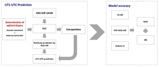
3. The Constrained PCF+WLS+AR Prediction Model

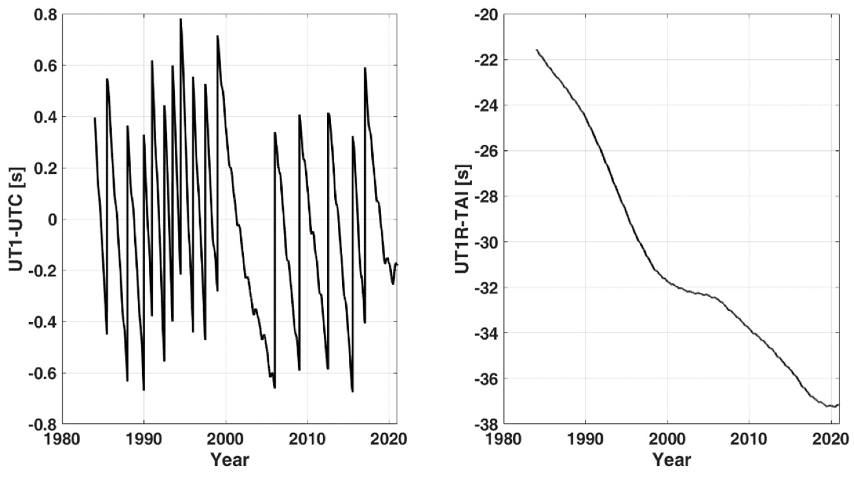
3.1. Data Description

The latest version of the EOP 14C04 was released by IERS on 1 February 2017 [28], and is available at http://hpiers.obspm.fr/eoppc/eop/eopc04/ (accessed on 3 May 2021). The new C04 is consistent with ITRF2014, and the EOPs have been updated since 1984. Figure 1 shows a comparison of UT1-UTC and UT1-TAI adopted by IERS from 1984 to now. Since existing studies have shown that the optimal base sequence length for UT1-UTC prediction is between 10 and 18 years [11,17,29,30], 12 years was chosen empirically as the base sequence length in this study.

3.2. Application of PCF in UT1R-TAI Modeling

The UT1R-TAI is a non-stationary series due to complex time variation. Based on the PCF algorithm, we extract trend terms from the original series to improve the applicability between the WLS+AR prediction model and the residual series. Figure 2 shows the fitted series and their residuals based on the LS and PCF algorithms for UTIR-TAI from 2000 to now, respectively. Compared with the LS fitting, the PCF has smaller fitted residuals, which are more consistent with the overall trend of UT1R-TAI series. After spectral analysis using fast Fourier transform (FFT), there are significant annual and semi-annual periodic terms in the PCF residuals shown in Figure 3.

For discrete data, the standard deviation (STD) of the fitted residuals is generally used to determine the optimal degree of PCF. The equation can be formed as follows:

$$S^2=\frac{1}{n-1}{{\displaystyle \sum _{i=1}^n\left(f_{pcf}(i)-O_{ut}(i)\right)}}^2$$

(13)

where $S$ is the standard deviation, $f_{pcf}$ is the fitted value of UT1R-TAI, and $O_{ut}$ is the original value of UT1R-TAI.

Figure 4 shows the standard deviation of PCF at different degrees for UT1R-TAI from 2000 to now. It is important to note that the standard deviation of the PCF residuals is basically constant after the degree reaching a threshold. As is well known, the curve will exhibit high-frequency oscillations with increasing degree, leading to overfitting. Therefore, the optimal PCF degree for UT1R-TAI since 2000 can be chosen as 8.

Considering that the UT1-UTC is susceptible to strong El Niño, which occurred three times after 2000 (i.e., 2006–2007, 2010–2011, 2014–2016), we separately determine the optimal PCF degree based on multiple sets of 12-year UT1-UTC series in this study.

As can be seen in Figure 5, the optimal PCF degree for the 12-year UT1-UTC series is smaller, with values between 4 and 8, than that for the 20-year series (shown in Figure 4). Another significant piece of information in Figure 5 is that the optimal degree for different base series is inconsistent, a fact which should be paid more attention in PCF extrapolation. The purpose of using PCF in this study is to improve the extrapolation accuracy of trend term in UT1R-TAI series, and multiple sets of experiments were carried out to further verify the accuracy of the optimal degree for PCF extrapolation.

Figure 6 shows the PCF extrapolation results of different degrees over six time periods. It can be seen that there is a big difference between the extrapolation results using a few fitting degrees with similar accuracy. The 1-year extrapolated values from 1 January 2014 using 4-, 6- and 8-degree PCF, from 1 January 2015 using 4-degree PCF, from 1 January 2016 using 4-, 5- and 7-degree PCF, from 1 January 2017 using 5- and 8-degree PCF, from 1 January 2018 using 5- and 6-degree PCF, and from 1 January 2019 using 4-degree PCF are in good agreement with the original observations. Compared with the results in Figure 5, the optimal fitting and extrapolation PCF degree based on the 12-year UT1R-TAI series are different, but 4- or 5-degree PCF have better accuracy in the two applications. In view of the difference of 12-year UT1-UTC series used in each prediction, the optimal degree for PCF extrapolation should be first determined. In this study, we first propose the annual constraint method to determine the optimal degree of PCF.

3.2.1. Determination of Degree of PCF by Annual Constraint Method

As shown in Figure 2, the long-term trends of the UT1R-TAI series approximate a straight line. Although there are still annual and semi-annual periodic terms in the PCF residuals, the residual values are relatively small compared to the observations, which is not considered in the determination of PCF degree. Therefore, we use the observations at the start time of the prediction and the previous span of time to constrain the prediction at the next span of time, as shown in Figure 7. Since the prediction span is 1 year in this study, this constraint method is defined as an annual constraint.

Using linear symmetry features [31], the constrained value can be obtained from

$$[UT1R-TA{I}_{pred}(T)]\approx [UT1R-TA{I^{\prime }}_c(T)]=2\ast [UT1R-TA{I}_{start}]-[UT1R-TA{I}_{obs}(-T)]$$

(14)

where $[UT1R-TA{I}_{pred}(T)]$ is the prediction value at a span of 365 days, $[UT1R-TA{I^{\prime }}_c(T)]$ is the constrained value, which is called the annual constraint. $[UT1R-TA{I}_{start}]$ is the prediction start time, $[UT1R-TA{I}_{obs}(-T)]$ is the observation from 365 days before the start time.

To verify the availability and accuracy of the annual constraint, the PCF+WLS+AR prediction model is established with a different degrees in this study, and the effects of different PCF degrees on the prediction results were compared with the 365-day UT1R-TAI prediction. According to the previous study (Figure 6), 4 or 5 is the optimal degree for PCF extrapolation in most cases. Therefore, the optimal PCF degree was selected as either 4 or 5 based on the annual constraint method, and the PCF+WLS+AR model was used to predict the UTIR-TAI in this study. Figure 8 shows a comparison of UT1R-TAI prediction in different time periods based on the PCF+WLS+AR model.

In Figure 8, the blue line represents the UT1R-TAI series, the green line is the constraint value (CV) series calculated based on the annual constraint method in this study, the thin black and red lines correspond to the prediction series based on the PCF+WLS+AR model on 4 and 5 degrees, respectively. Comparing the predictions and constraint values for the 365-day span, we selected the optimal PCF degree according to the closest to constraint values principle. In addition, we also compared the optimal degree prediction with the original series at different time periods and determined an identification as either T or F. As can be seen in

Table 1. The chosen degree of PCF depends on the predictive constraint method.

Time	Optimal Degree of PCF by Annual Constraint	True/False
1 January 2014	4	T
1 July 2014	4	T
1 January 2015	4	T
1 July 2015	5	T
1 January 2016	5	T
1 July 2016	5	T
1 January 2017	5	T
1 July 2017	5	T
1 January 2018	4	F
1 July 2018	4	T

, the predictions of degree selected based on the annual constraint are optimal for most of the time periods, except for 1 January 2018. This may be due to the fact that UT1-UTC is affected by the internal and external factors of the Earth, deviating sharply from the original trend during 2018–2019. Therefore, we need to further optimize the selection strategy for PCF degree.

3.2.2. Optimization of PCF Degree Using the Interval Constraint Method

As shown in the previous analysis, UT1-UTC may exhibit violent oscillations in the series, with a serious influence of internal and external factors at a certain stage, resulting in large errors in the annual constraint method. Therefore, in this study, the interval constraint method is introduced to further optimize the determination of PCF degree by calculating the annual variation.

Figure 9 shows the annual increment of the UT1R-TAI from 2000 to 2014. It can be seen that the annual variation of UT1R-TAI from 2000 to 2006 is relatively small, about −0.05 s~−0.2 s. However, the annual increment of UT1R-TAI suddenly decreased to −0.3 s~−0.4 s in 2007, and remained at this magnitude for several years thereafter. Considering the strong El Niño that occurred in 2006, this drastic variation may have been caused by this event. The real cause is beyond the scope of this study, and will not be studied in detail. In addition, it is not difficult to find that the mean annual variation of UT1R-TAI is about −0.3 s, with a fluctuation of 0.15 s. Therefore, −0.3 0.15 s can be chosen as the constraint interval for annual increment. The annual constraint method determines the PCF degree N (4 or 5) based on the difference between the annual prediction value and the CV, while the interval constraint method optimizes the PCF degree on the basis of the difference between the annual prediction value and the prediction starting value, i.e., the predicted annual increment. N is the optimal degree if the predicted annual increment is within the constraint interval. In other cases, the optimal PCF degree is the one closed to the prediction annual increment of −0.3 s, when the prediction annual increments based on the PCF+WLS+AR model with degree 4 and 5 are both outside the interval. Additionally, when the results of the annual constraint and interval constraint methods are inconsistent, the optimal degree based on the interval constraint is preferred.

3.3. The Processing of the Constrained PCF+WLS+AR Model

In this study, we proposed the model for UT1-UTC prediction as shown in Figure 10. The prediction process is demonstrated by the following steps.

(1)

Determination of the PCF model.

• Based on the annual constraint method, the CV is calculated and compared with the annual prediction value to determine the initial optimal PCF degree;
• Optimize with interval constraints to obtain the final optimal PCF degree;
• Use the optimal degree for polynomial curve fitting and extrapolation.

(2)

Construction of WLS model.

4.

Model the residuals of PCF and obtain the WLS extrapolation.

(3)

Residual prediction based on AR model.

5.

Model the residuals of WLS.

(4)

UT1-UTC prediction using the combined PCF+WLS+AR model.

6.

Add the leap seconds and solid Earth zonal tides.

It is important to note that Pre_O_s is the difference between the PCF+WLS+AR model on degree 4/5 and the UT1R-TAI value at the starting point and Fit_O_s is the difference between the PCF model and the UT1R-TAI value at the starting point of prediction.

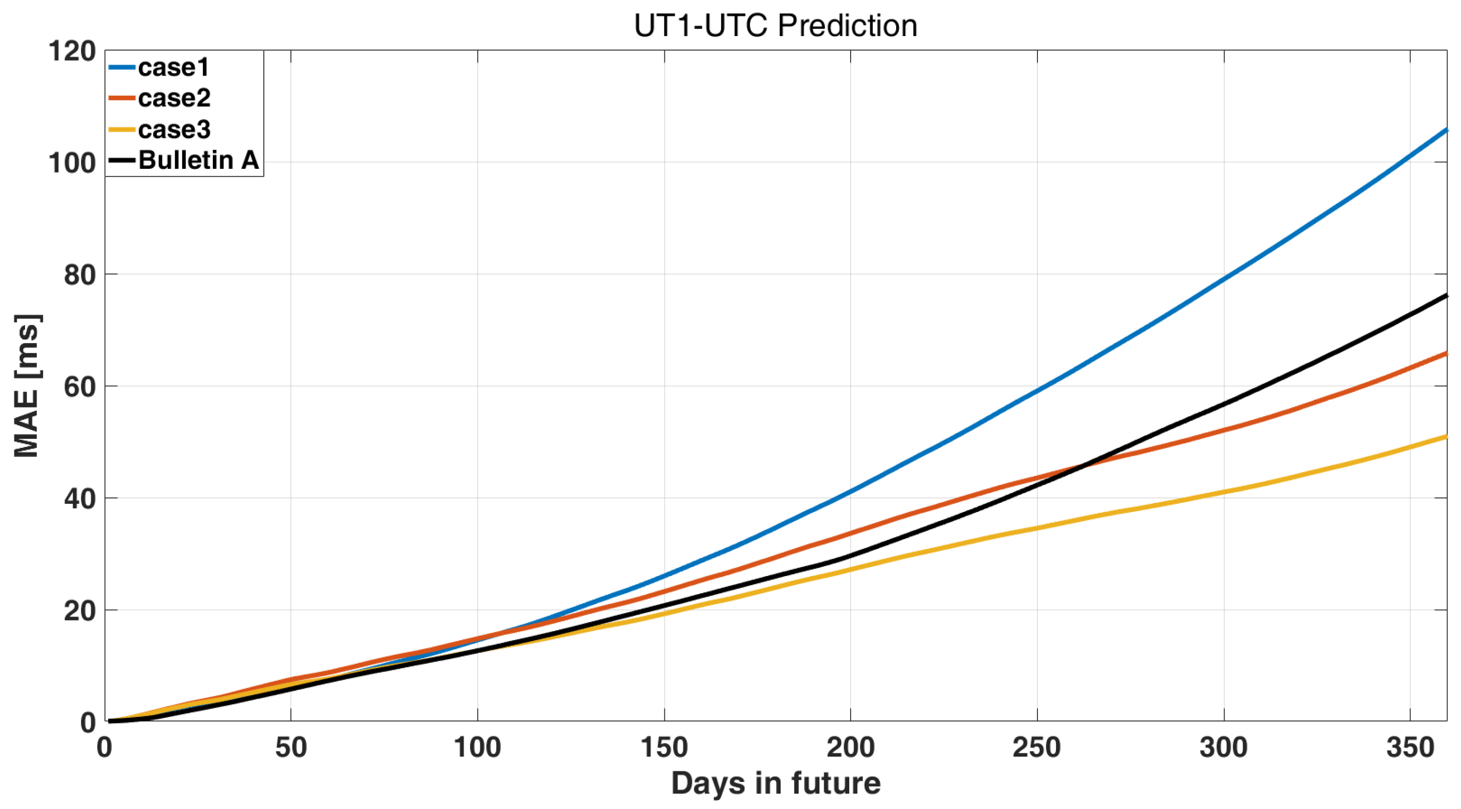
4. Results and Discussion

In this study, the accuracy of the constrained PCF+WLS+AR prediction model was validated based on multiple sets of prediction experiments using the EOP 14C04 series between 2014 and 2019. The experimental scheme was as follows.

• Case 1: UT1-UTC prediction based on the LS+AR model;
• Case 2: UT1-UTC prediction based on the constrained PCF+WLS+AR model (considering annual constraint);
• Case 3: UT1-UTC prediction based on the constrained PCF+WLS+AR model (considering annual constraint and interval constraint);
• Case 4: Bulletin A results achieved by IERS.

The four cases above represent the LS+AR model, the two PCF+WLS+AR models proposed in this paper, and Bulletin A provided by IERS, respectively. The prediction span was 360 days with a weekly sliding window, and the accurate statistical period was from 3 January 2014 to 6 August 2019. Figure 11 shows the MAE of UT1-UTC prediction in four cases. Compared to the other models, the MAE of the proposed constrained PCF+WLS+AR models exhibited fewer errors in mid- and long-term prediction (90~360 days). Since the PCF+WLS+AR model better takes into account the overall trend of the base series, it obtains a more accurate long-term trend and long-period term than the LS model during extrapolation, thus improving the mid- and long-term UT1-UTC prediction accuracy. Combined with the UT1-UTC prediction accuracy statistics presented in

Table 2. Comparison of prediction accuracy for 4 cases with the unit [ms]. The improvement represents the prediction accuracy of Case 3 relative to Case 4.

Span	Case 1	Case 2	Case 3	Case 4	Improvement
1	0.036	0.037	0.036	0.056	35.5%
10	1.049	1.124	1.083	0.452	−139.4%
20	2.460	2.749	2.596	1.601	−62.1%
30	3.544	4.151	3.802	2.910	−30.7%
60	7.396	8.722	7.616	7.284	−4.6%
90	12.390	13.191	11.332	11.271	−0.5%
120	18.338	17.867	15.077	15.626	3.5%
180	33.148	29.346	23.954	25.962	7.7%
240	51.349	41.785	33.250	39.485	15.8%
300	71.272	52.021	40.979	56.666	27.7%
360	92.197	65.819	50.934	76.217	33.2%

, the improvement value relative to Bulletin A was positive after 90 days in the future, and the improvement gradually increased with the progression of the prediction span, reaching a maximum of 33.2%. However, for short-term prediction, Bulletin A showed a smaller MAE in the four cases. As shown in Table 2, it can be seen that Bulletin A clearly outperformed the other models in terms of short-term prediction, especially the first 20 days in the future. This advantage is primarily due to the fact that Bulletin A takes into account the effects of Atmospheric Angular Momentum (AAM) and Oceanic Angular Momentum (OAM). Kalarus et al. [1] showed that the main contribution of AAM and OAM to UT1-UTC is its high-frequency component. Therefore, the additional inputs, i.e., AAM and OAM, can improve the modeling of the high-frequency component of UT1-UTC, thus improving the short-term prediction accuracy of UT1-UTC. Compared with the LS+AR model, except that the first 60 days of future have basically similar accuracy, the PCF+WLS+AR model demonstrates a more obvious improvement in terms of mid- and long-term prediction.

Figure 12 presents the Absolute Errors (AE) of 360-day prediction between 2014 and 2019 for these four cases in order to better understand the prediction performance and its causes. It can be seen that the PCF+WLS+AR model considering annual constraint and interval constraint demonstrates a significant improvement in mid- and long-term UT1-UTC prediction accuracy compared to the LS+AR model and Bulletin A. In the results of Bulletin A, the long-term prediction from the beginning of 2015 has high errors, which may have been caused by the superstrong El Niño warm event occurring between 2015 and 2016. Obviously, our proposed method was effective for prediction with high accuracy during this period. This is due to the fact that we accurately fit the base series and continuously optimize the polynomial degree by means of annual and interval constraints to obtain the optimal extrapolation values. However, with the time-varying of PCF degree, there is also a sudden change in adjacent starting prediction errors.

5. Conclusions

UT1-UTC is a quantitative parameter describing the Earth’s rotation rate, which is the most difficult to predict in the five EOPs due to the complex and variable periodic term. Among existing prediction models, LS is the most widely used for fitting trend terms and periodic terms. In this study, based on the characteristics of UT1-UTC and its inherent periodic and trend terms, a constrained PCF+WLS+AR prediction model is proposed. The proposed model fully takes into account the trend and long-period terms of the UT1R-TAI series, as well as its annual variation and the strong influence of recent data. This is an important enhancement to high-precision modeling and PCF extrapolation. To obtain the optimal PCF degree, we introduce two constraint methods, namely annual constraint and interval constraint. Finally, multiple sets of prediction experiments based on EOP 14C04 series were carried out to verify the accuracy of this proposed model. The comparison with prediction accuracy of other methods indicates that the constrained PCF+WLS+AR model can efficiently and precisely predict the UT1-UTC in the middle and long term. Compared to Bulletin A, released by IERS, the proposed model demonstrates improved accuracy of UT1-UTC prediction by up to 33.2% in the middle and long term (90–360 days). However, Bulletin A demonstrates much smaller errors in short-term prediction, especially in the ultra-short term.

Future work may focus on the strong relation between AAM, OAM, and UT1-UTC. A prediction model such as the constrained PCF+WLS+MAR, based on multiple inputs of EOP, AAM and OAM, will be established to improve short-term UT1-UTC prediction accuracy. At the same time, a better constraint method for PCF needs to be further explored.

References

1. Kalarus, M.; Schuh, H.; Kosek, W.; Akyilmaz, O.; Bizouard, C.; Gambis, D.; Gross, R.; Jovanović, B.; Kumakshev, S.; Kutterer, H.; et al. Achievements of the Earth orientation parameters prediction comparison campaign. J. Geod. 2010, 84, 587–596. [Google Scholar] [CrossRef]
2. Schuh, H.; Ulrich, M.; Egger, D.; Müller, J.; Schwegmann, W. Prediction of Earth orientation parameters by artificial neural networks. J. Geod. 2002, 76, 247–258. [Google Scholar] [CrossRef]
3. Schuh, H.; Behrend, D. VLBI: A fascinating technique for geodesy and astrometry. J. Geodyn. 2012, 61, 68–80. [Google Scholar] [CrossRef] [Green Version]
4. Pearlman, M.R.; Degnan, J.J.; Bosworth, J.M. The international laser ranging service. Adv. Space Res. 2002, 30, 135–143. [Google Scholar] [CrossRef]
5. Hein, G.W. Status, perspectives and trends of satellite navigation. Satell. Navig. 2020, 1, 22. [Google Scholar] [CrossRef]
6. Willis, P.; Fagard, H.; Ferrage, P.; Lemoine, F.G.; Noll, C.E.; Noomen, R.; Otten, M.; Ries, J.C.; Rothacher, M.; Soudarin, L. The international DORIS service (IDS): Toward maturity. Adv. Space Res. 2010, 45, 1408–1420. [Google Scholar] [CrossRef]
7. Gambis, D. Monitoring Earth orientation using space-geodetic techniques: State-of-the-art and prospective. J. Geod. 2004, 78, 295–303. [Google Scholar] [CrossRef]
8. Nilsson, T.; Heinkelmann, R.; Karbon, M.; Raposo-Pulido, V.; Soja, B.; Schuh, H. Earth orientation parameters estimated from VLBI during the CONT11 campaign. J. Geod. 2014, 88, 491–502. [Google Scholar] [CrossRef]
9. Gross, R.S.; Marcus, S.L.; Eubanks, T.M.; Dickey, J.O.; Keppenne, C.L. Detection of an ENSO signal in seasonal length-of-day variations. Geophys. Res. Lett. 1996, 23, 3373–3376. [Google Scholar] [CrossRef]
10. Kosek, W.; Kalarus, M.; Johnson, T.; Wooden, W.; McCarthy, D.; Popinski, W. A comparison of UT1-UTC forecasts by different prediction techniques. Proc. Journeys Syst. Ref. Spatiotemporal 2004, 140–141. [Google Scholar]
11. Niedzielski, T.; Kosek, W. Prediction of UT1–UTC, LOD and AAM χ3 by combination of least-squares and multivariate stochastic methods. J. Geod. 2007, 82, 83–92. [Google Scholar] [CrossRef]
12. McCarthy, D.D.; Petit, G. IERS Conventions (2003); International Earth Rotation And Reference Systems Service (IERS): Cologne, Germany, 2004. [Google Scholar]
13. Kosek, W.; Kalarus, M.; Johnson, T.; Wooden, W.; McCarthy, D.; Popinski, W. A comparison of LOD and UT1-UTC forecasts by different combined prediction techniques. Artif Satell 2005, 40, 119–125. [Google Scholar]
14. Kosek, W.; McCarthy, D.; Luzum, B. Possible improvement of Earth orientation forecast using autocovariance prediction procedures. J. Geod. 1998, 72, 189–199. [Google Scholar] [CrossRef]
15. Gross, R.S.; Eubanks, T.M.; Steppe, J.A.; Freedman, A.P.; Dickey, J.O.; Runge, T.F. A Kalman-filter-based approach to combining independent Earth-orientation series. J. Geod. 1998, 72, 215–235. [Google Scholar] [CrossRef]
16. Kosek, W. Future Improvements in EOP Prediction; Springer: Berlin/Heidelberg, Germany, 2012; pp. 513–520. [Google Scholar]
17. Xu, X.Q.; Zhou, Y.H.; Liao, X.H. Short-term earth orientation parameters predictions by combination of the least-squares, AR model and Kalman filter. J. Geodyn. 2012, 62, 83–86. [Google Scholar] [CrossRef]
18. Dill, R.; Dobslaw, H.; Thomas, M. Improved 90-day Earth orientation predictions from angular momentum forecasts of atmosphere, ocean, and terrestrial hydrosphere. J. Geod. 2018, 93, 287–295. [Google Scholar] [CrossRef] [Green Version]
19. Chen, J.; Wilson, C. Hydrological excitations of polar motion, 1993–2002. Geophys. J. Int. 2005, 160, 833–839. [Google Scholar] [CrossRef] [Green Version]
20. Shen, Y.; Guo, J.Y.; Liu, X.; Kong, Q.L.; Guo, L.X.; Li, W. Long-term prediction of polar motion using a combined SSA and ARMA model. J. Geod. 2018, 92, 333–343. [Google Scholar] [CrossRef]
21. Zheng, D.; Chao, B.; Zhou, Y.; Yu, N. Improvement of edge effect of the wavelet time–frequency spectrum: Application to the length-of-day series. J. Geod. 2000, 74, 249–254. [Google Scholar] [CrossRef]
22. Burden, R.L.; Faires, J.D.; Burden, A.M. Numerical Analysis; Cengage Learning: Boston, MA, USA, 2015. [Google Scholar]
23. Keren, D.; Gotsman, C. Fitting curves and surfaces with constrained implicit polynomials. IEEE Trans. Pattern Anal. Mach. Intell. 1999, 21, 31–41. [Google Scholar] [CrossRef] [Green Version]
24. Peck, J. Polynomial curve fitting with constraint. SIAM Rev. 1962, 4, 135–141. [Google Scholar] [CrossRef]
25. Sun, Z.; Xu, T. Prediction of earth rotation parameters based on improved weighted least squares and autoregressive model. Geod. Geodyn. 2012, 3, 57–64. [Google Scholar]
26. Weisstein, E.W. Least Squares Fitting. 2002. Available online: https://mathworld.wolfram.com/ (accessed on 10 July 2020).
27. Cohen, A.; Migliorati, G. Optimal weighted least-squares methods. SMAI J. Comput. Math. 2017, 3, 181–203. [Google Scholar] [CrossRef]
28. Bizouard, C.; Lambert, S.; Gattano, C.; Becker, O.; Richard, J.-Y. The IERS EOP 14C04 solution for Earth orientation parameters consistent with ITRF 2014. J. Geod. 2019, 93, 621–633. [Google Scholar] [CrossRef]
29. Jia, S.; Xu, T.H.; Sun, Z.Z.; Li, J.J. Middle and long-term prediction of UT1-UTC based on combination of Gray Model and Autoregressive Integrated Moving Average. Adv. Space Res. 2017, 59, 888–894. [Google Scholar] [CrossRef]
30. Modiri, S.; Belda, S.; Hoseini, M.; Heinkelmann, R.; Ferrándiz, J.M.; Schuh, H. A new hybrid method to improve the ultra-short-term prediction of LOD. J. Geod. 2020, 94, 23. [Google Scholar] [CrossRef] [Green Version]
31. Bigun, J. Optimal Orientation Detection of Linear Symmetry; Linköping University Electronic Press: Linköping, Sweden, 1987. [Google Scholar]
Figure 1. The UT1−UTC and UT1R−TAI series from 1984 to now (data from IERS website).
Remotesensing 14 03252 g001
Figure 2. The original UT1R−TAI series and its two fitting series with different residuals since 2000.
Remotesensing 14 03252 g002
Figure 3. Frequency spectrum of the PCF residuals based on UT1R-TAI using fast Fourier transform (FFT).
Remotesensing 14 03252 g003
Figure 4. The STD of PCF at different degrees for UT1R-TAI from 2000 to now.
Remotesensing 14 03252 g004
Figure 5. The standard deviation of PCF at different degrees for UT1R−TAI of 12 years.
Remotesensing 14 03252 g005
Figure 6. Comparison of polynomial curve fitting at different degrees for extrapolation. D4, D5, D6, D7 and D8 represent the fitted and extrapolated results of the original series with 4-, 5-, 6-, 7- and 8-degree PCF, respectively.
Remotesensing 14 03252 g006
Figure 7. The distribution of points in predictive constraint method.
Remotesensing 14 03252 g007
Figure 8. The comparison of UT1R−TAI prediction in different time periods based on the PCF+WLS+AR model.
Remotesensing 14 03252 g008
Figure 9. The annual increment of UT1R-TAI from 2000 to 2014.
Remotesensing 14 03252 g009
Figure 10. The process of the PCF+WLS+AR prediction model.
Remotesensing 14 03252 g010
Figure 11. Mean absolute errors (MAE) of the UT1-UTC prediction using 4 cases with the unit [ms]. Case 1, Case 2, and Case 3 denote the LS+AR model (blue line), the PCF+WLS+AR model with annual constraints (orange line), and the PCF+WLS+AR model with annual and interval constraints (yellow line), respectively. Bulletin A is indicated by the black line.
Remotesensing 14 03252 g011
Figure 12. Absolute errors (in mas) of the UT1-UTC prediction using LS+AR model, the PCF+WLS+AR model with annual constraints, the PCF+WLS+AR model with annual and interval constraints and Bulletin A. The four subplots represent the prediction accuracy of Case 1, Case 2, Case 3, and Case 4 from top to bottom.
Remotesensing 14 03252 g012