Joint Classification of Hyperspectral and LiDAR Data Based on Position-Channel Cooperative Attention Network

Abstract

Remote sensing image classification is a prominent topic in earth observation research, but there is a performance bottleneck when classifying single-source objects. As the types of remote sensing data are gradually diversified, the joint classification of multi-source remote sensing data becomes possible. However, the existing classification methods have limitations in heterogeneous feature representation of multimodal remote sensing data, which restrict the collaborative classification performance. To resolve this issue, a position-channel collaborative attention network is proposed for the joint classification of hyperspectral and LiDAR data. Firstly, in order to extract the spatial, spectral, and elevation features of land cover objects, a multiscale network and a single-branch backbone network are designed. Then, the proposed position-channel collaborative attention module adaptively enhances the features extracted from the multi-scale network in different degrees through the self-attention module, and exploits the features extracted from the multiscale network and single-branch network through the cross-attention module, so as to capture the comprehensive features of HSI and LiDAR data, narrow the semantic differences of heterogeneous features, and realize complementary advantages. The depth intersection mode further improves the performance of collaborative classification. Finally, a series of comparative experiments were carried out in the 2012 Houston dataset and Trento dataset, and the effectiveness of the model was proved by qualitative and quantitative comparison.

1. Introduction

With the continuous development of remote sensing technology, remote sensing images are rich in high-resolution ground information, and remote sensing image classification is an important component of remote sensing interpretation, which is widely used in natural disaster prevention, urban and rural planning and other fields. Remote sensing image classification extracts the high-level semantic information of images, and maps the features of remote sensing images to category labels, to realize the classification and recognition of images [1]. Among multitudinous remote sensing data, hyperspectral images (HSI) are obtained by imaging spectrometer, with wavelengths that cover visible and near-infrared channels, reflecting spectra of hundreds/thousands of bands of each pixel on the earth’s surface, narrower spectral bands, and more channels [2]. HSIs have spatial and spectral smoothness, which can not only describe objects in detail and accurately, but also has a high correlation between adjacent bands, greatly improving the ability of target recognition [3,4,5].

However, the intense correlation of HSI will lead to information redundancy. When sensors collect HSI scene data, they are easily interfered by environmental factors, such as clouds and shadows, which will be prone to cause information confusion. Therefore, HSI alone can hardly yield promising classification results. Compared with HSI, light detection and ranging (LiDAR) uses pulsed laser to measure the range, which is an active remote sensing method [6,7]. Moreover, LiDAR is not easily affected by weather conditions, which can not only provide the height and shape information of the scene, but also has intense accuracy and flexibility [8,9]. HSIs can provide various spectral information, and LiDAR data has accurate spatial and elevation information. The two data are deeply fused to realize the complementary advantages of multi-source remote sensing data, thus breaking through the performance bottleneck of single remote sensing data (such as “foreign objects with the same spectrum” or “same object with different spectrums”) and finally achieving the purpose of improving the classification accuracy of objects [10,11]. Many works of literature have proven the effectiveness of the combined interpretation of HSI and LiDAR, indicating that LiDAR can make up for the shortcomings of HSI sensors to some extent. For HSI classification, a series of classification methods have been proposed, such as support vector machines (SVMs) [12], which are widely used in the case of less training data, extreme learning machine [13], random forest classification [14], classification based on sparse representation [15,16,17], evidence theory [18,19,20], etc. Morphological extended attribute profiles (EAPs) can be used for joint feature extraction of HSI and LiDAR images to achieve the purpose of classification [21]. In [22], using multi-kernel learning combined with multi-source heterogeneous features, the kernels constructed by different features are weighted summation. Ge et al. combined classification of HSI and LiDAR images by extinction profiles (EPs), local binary pattern (LBP), and kernel collaborative representation [23]. In [24], the extended multi-attribute profile (EMAP) is used for feature extraction, multi-scale total variation (MSTV) is used for feature estimation in low-dimensional space, and the random forest classifier is used for classification finally. ShearSAF [25] transforms the reduced dimension HSI and LiDAR images into Shearlet domain for feature extraction, and finally classifies them through the random forest.

Most of the traditional classification models simply stack the features of multimodal data, and the direct superposition of these high-dimensional features leads to Hughes phenomenon inevitably. Additionally, the traditional methods of classification rely heavily on hand-designed features, which limis the expression of the model [26]. Of late years, convolutional neural network (CNN) has been proved to be effective in many computer vision tasks, such as classification [27,28,29], detection [30], and segmentation [31]. The research method based on CNN model has become the mainstream method in the field of remote sensing image classification [32,33], showing excellent feature extraction ability and gradually replacing the method based on manual features.

The IEEE GRSS data fusion contest provided data support for multi-source remote sensing image fusion, and accelerated the development of data fusion technology. Li et al. [34] constructed three CNNs to learn the spectral, spatial, and altitude characteristics, respectively, and then fused them using the composite kernel method. To solve the problem caused by feature imbalance, the step of feature fusion is skipped, and a decision fusion method of HSI and LiDAR data classification is proposed [35]. In [36,37], both feature fusion strategy and decision fusion strategy are used to improve the classification performance. Although these methods have been proved to be effective, the complementarity and heterogeneity between HSI and LiDAR data lead to great differences in object representation, and it is difficult to achieve satisfactory classification performance with a plot of training samples. To dispose of this problem, unsupervised CNN models based on encoder–decoder architecture were proposed [38,39], and the data reconstruction strategy is certified to capacity for better activating the neurons across modalities. In [40], the two-branch convolutional neural network combines the spatial and spectral features of HSI extracted separately with the features extracted by LiDAR. EndNet [41] is a deep encoder–decoder network architecture, which can reconstruct multimodal input by enforcing fusion features. In [42], MDL-Middle is an intermediate fusion CNN model. Zhang et al. [43] put forward an interleaving perception convolutional neural network (IP-CNN), designed a bidirectional self-encoder to reconstruct multimodel data, and integrated multi-source heterogeneous information in an interleaving manner. In addition, attention mechanisms have been successfully applied to remote sensing image classification.

Attention mechanism originates from visual signal processing, which indicates the strategy of allocating biased computing resources to the processed signal to underline its information. In the observation of scene or image information, attention will make our brain specialize in the target area, highlight the salient features and suppress the irrelevant features, which is extensively used in classification tasks. In 2017, the Google team put forward the self-attention structure in the article “Attention is all you need” [44], which caused a huge response, making the attention mechanism an important research topic. Hu et al. [45] proposed Squeeze-and-Excitation (SE), which can make the network pay attention to the relationship between channels, and automatically learn the importance of different channel features, improving the accuracy of image classification. The convolutional block attention module (CBAM) proposed by Woo et al. [46] and the attention module (BAM) proposed by Jong et al. [47] can consider both spatial attention and channel attention at the same time when used in image classification, it can make the error rate lower and the classification more stable.

An attention module can be introduced into the model to pay close attention to significant features in channel and position. Fu et al. [48] proposed the double attention network (DAN), which proposed the position attention module and the channel attention module to establish the semantic dependency and applied it to the multimodal fusion network of HSI and LiDAR classification. FusAtNet was proposed in [49], similar to the method in this paper, the model highlights the spectral features of HSI by self-attention mechanism, and fuses the spatial features of LiDAR by cross-attention mechanism. ${\mathrm{S}}^2\mathrm{ENet}$ [50] proposed ${\mathrm{S}}^2\mathrm{EM}$ module for spatial–spectral enhancement of cross-modal information interaction. However, there are still some problems with these methods. The features are only fused in the shallow layer, which does not fully reflect the complementarity of HSI and LiDAR features. In this paper, by combining attention mechanism, a joint classification of HSI and LiDAR data based on the position-channel cooperative attention network is proposed. The different levels of features are extracted through the multiscale network, and deep fusion is carried out through the position-channel cooperative attention (${\mathrm{PC}}^2\mathrm{A}$) module, so as to give full play to the complementary advantages of multimodal data.

In this article, we propose a joint classification of HSI and LiDAR data based on position-channel cooperative attention network. In feature extraction, we use a multiscale network and self-position enhancement attention network to extract different levels of deep features of HSI. Then, a forward-inverted CNN structure is designed to extract rich spatial features of LiDAR images, and it is fused with the extracted HSI features to obtain spatial–spectral information among different levels. Finally, the probability distribution of each pixel is calculated by three classification modules, and the classification results are fused. The effectiveness of the proposed model is proved on real HSI data sets.

The main contributions are summarized as follows:

• A multiscale network is designed to obtain different level of location channel features, and design a single-branch network to extract rich position information of LiDAR;
• The effective ${\mathrm{PC}}^2\mathrm{A}$ module is designed, which consists of three modules: self-position enhancement attention (SPA), fused-position enhancement attention (FPA) and fused-channel enhancement attention (FCA). Enhanced features obtained through ${\mathrm{PC}}^2\mathrm{A}$ module can make full use of the complementarity of position-channel features of HSI and LiDAR images, and the fused features are helpful to obtain more effective classification results;
• In the fusion phase, shallow features are fused by the position-channel cooperative attention network, and then the deep features are fused by concatenation mechanism. To enhance the identification ability of learned features, three output layers are adopted, and these three output results are combined via a weighted summation method, whose weights are automatically updated through the network learning.

The rest of this article is organized as follows. The details of the proposed model are described in Section 2. In Section 3, the data set and experimental results are introduced. Finally, this article is summarized in Section 4.

2. Methodology

2.1. Overview

The framework of the proposed position-channel collaborative attention network (${\mathrm{PC}}^2\mathrm{ANet}$) is shown in Figure 1, including the feature extraction model, ${\mathrm{PC}}^2\mathrm{A}$ module, and decision fusion module. The feature extraction model consists of a multiscale network and a single-branch network. The multiscale network uses 2D CNN and 3D CNN with different kernel sizes to extract the position and channel information of HSI, and the 2D CNN is used in a single-branch network to extract the position information of LiDAR. ${\mathrm{PC}}^2\mathrm{A}$ module consists of SPA, FPA, and FCA. The SPA module can enhance the spatial features of HSI, besides, the FPA and FCA module can enhance the spatial features of HSI and the channel features of LiDAR through cross-attention. Data fusion methods include feature fusion and decision fusion. Among them, feature fusion is the fusion of extracted HSI features and LiDAR features through feature concatenate, and decision fusion consists of three classification modules.

2.2. Feature Extraction Model

The overall parameter configuration of the designed feature extraction model is described in detail in Figure 2. In the classification task, a large number of samples are needed for training. However, the collection of ground reference data is expensive and difficult, so it is difficult to obtain a large number of ground reference data. Moreover, the manual labeling of HSI is costly, so there are few labeled samples available. To solve this problem, the existing training samples are rotated to expand the sample set.

After the data rotated, the HSI feature is fed into the multiscale network, which includes 3D CNN, 2D CNN, batch normalization layers, and ReLU. Two-dimensional CNN can fully extract spatial information, but will ignore the rich spectral features of HSIs. Three-dimensional CNN can extract spatial and spectral information, but excessive use will make the network too bloated, which may reduce the classification accuracy. In order to alleviate these problems, the combination of 3D CNN and 2D CNN is used to construct a multiscale network for feature extraction of HSI in this paper. Each branch has different hierarchical structures, and the first convolutional layer of each branch has a different kernel size. Three different features are extracted by different branches, and then they are fused after passing through the SPA module, respectively, so that more discriminative feature representation can be obtained, and the classification performance can be effectively improved.

The LiDAR image feature is fed into a single-branch network, which includes 2D CNN, batch normalization layers, and ReLU. LiDAR images contain abundant spatial information, which can make up for the low spatial resolution of HSI. Three-layer 2D CNN is used to extract spatial features of LiDAR. Through feature extraction, the number of channels of LiDAR images is continuously deepened, so as to further integrate with the features extracted by HSI.

2.3. Position-Channel Collaborative Attention Module

(1) Self-Position Attention Module: Self-position attention module can build rich semantic associations on local features to realize the spatial enhancement of HSI. The features A, B, and C are extracted from the three branches of the multi-scale network, respectively. The spatial and spectral features of HSI images are extracted in different degrees, but the spatial features of HSI images are not significant enough. The SPA module can be used to strengthen the spatial details of three branches, and transmit A, B, and C to the SPA module, respectively, which makes the spatial features more discriminating. Take feature A as an example, As shown in Figure 3a, given a local feature $A\in {\mathbb{R}}^{C\times H\times W}$, where $H\times W$ is the number of pixels and C is the number of channels. We first transpose it to $A^T\in {\mathbb{R}}^{H\times W\times C}$, then we perform a matrix multiplication between $A^T$ and A to calculate position attention map $B\in {\mathbb{R}}^{C\times C}$. After that, we aggregate the global vectors by the squeeze operation to obtain the position impact of all images corresponding to HSI. The whole process can be formulated as:

$$spa\left(A\right)=A\otimes Squ\left(g\left(A_i,A_0^T\right),\dots ,g\left(A_i,A_{(N-1)}^T\right)\right)$$

(1)

where $A\in {\mathbb{R}}^{C\times H\times W}$ is the extracted HSI image feature. $A_i\in {\mathbb{R}}^{1\times (H\times W)}$ and $A_j^T\in {\mathbb{R}}^{H\times W\times 1}$ denote the vectors at position i of A and position j of $A^T$, respectively. $Squ(·)$ represents squeeze operation. We define the function $g(·)$ as:

$$g\left(A,A^T\right)=R_1\left(A\right)·R_1\left(A^T\right)$$

(2)

where $R_1(·)$ denote dimensional transformation, which is reshaping three-dimensional space ${\mathbb{R}}^{C\times H\times W}$ into two-dimensional space ${\mathbb{R}}^{C\times (H\times W)}$. Features B and C, respectively, repeat the above operations to obtain three enhanced HSI features, and then fuse them by feature concatenate. The output of three SPA modules are calculated as:

$$outpu{t}^{(T-\mathrm{branch})}=Cat(spa\left(A\right),spa\left(B\right),spa\left(C\right))$$

(3)

where $Cat(·)$ denote concatenate, which is to splice two tensors together.

(2) Fused-Position Attention Module: FPA module can realize spatial enhancement of HSI through LiDAR image. This module captures the position response between HSI and LiDAR image features, and enhances the original HSI features through this response, so that the obtained features not only have rich channel information, but also have rich position information through enhancement. As shown in Figure 3b, given features $F_1\in {\mathbb{R}}^{C\times H_1\times W_1}$ and $F_2\in {\mathbb{R}}^{C\times H_2\times W_2}$, which represent the extracted HSI image features and LiDAR image features respectively. Firstly, we reshape $F_1\in {\mathbb{R}}^{C\times H_1\times W_1}$ into $F_1^T\in {\mathbb{R}}^{\left(H_1\times W_1\right)\times C}$, and perform dimensional tranformation and a matrix multiplication between $F_1^T$ and $F_2$ to get the position attention map $P\in {\mathbb{R}}^{\left(H_1\times W_1\right)\times \left(H_2\times W_2\right)}$. Through the squeeze operation, $F_1$ can obtain the spatial enhancement from all positions of $F_2$. The whole process can be formulates as:

$$fpa\left(F_1,F_2\right)=F_1\otimes Squ\left(g\left(f_1^i,f_2^0\right),\dots ,g\left(f_1^i,f_2^{N_2-1}\right)\right)$$

(4)

where $F_1\in {\mathbb{R}}^{C\times H_1\times W_1}$ is the extracted HSI image feature, $N_2=H_2\times W_2$. $f_1^i$ and $f_2^j$ denote the vectors at position i of $F_1^T$ and position j of $F_2$, respectively.

(3) Fused-Channel Attention Module: Correspondingly, the FCA module can realize channel enhancement of LiDAR image through HSI. This module captures the channel response between HSI and LiDAR image features, and enhances the original LiDAR image features through this response. As shown in Figure 3c, the spatial enhancement effect is calculated as:

$$fca\left(F_1,F_2\right)=F_2\otimes Squ\left(g\left(f_2^i,f_1^0\right),\dots ,g\left(f_2^i,f_1^{C_1-1}\right)\right)$$

(5)

where $f_2^i$ and $f_1^i$ denote the vectors at position i of $F_2^T$ and position j of $F_1$, respectively.

The two outputs of the multi-branch network model are the common inputs of the FPA module and the FCA module. FPA module is used to enhance the spatial features of HSI features, and the FCA module is used to enhance the channel representation of LiDAR features, and then the output of the single branch network is fused by feature addition. The calculation is as:

$$outpu{t}^{(S-\mathrm{branch})}=fpa\left(F_1,F_2\right)\oplus fca\left(F_1,F_2\right)$$

(6)

where ⊕ denotes the matrix addition, $F_1\in {\mathbb{R}}^{C\times H_1\times W_1}$ and $F_2\in {\mathbb{R}}^{C\times H_2\times W_2}$ represent the extracted HSI features and LiDAR image features, respectively.

2.4. Data Fusion Network Model

The data fusion method includes two parts, feature fusion, and decision fusion. Among them, feature fusion is the concatenate of HSI features extracted by the multiscale network and LiDAR features extracted by a single-branch network. Decision fusion is to fuse different classification results by adding weights, mainly the classification results after the SPA module, FPA and FCA module, and feature fusion.

The calculation process of feature fusion can be formulated as:

$$Out=Cat\left(\sigma \left({output}^{(M-branch)}\right),{output}^{(S-branch)}\right)$$

(7)

The calculation process of $\sigma (·)$ is as follows:

$$\sigma (·)=ReLU\left(BN\left(f_0(·)\right)\right)$$

(8)

where $BN(·)$ denotes batch normalization and $ReLU(·)$ denotes activation function. $f_0(·)$ denotes 2D convolution operation, which is to reduce the dimension of the features extracted by HSI for feature fusion.

The calculation process of classification module can be formulated as:

$$C(·)=MLP\left(Flatten\right(AvgPool(·)\left)\right)$$

(9)

$output{}^{(M-branch)}$ represents the output of HSI feature extraction network, $output{}^{(S-branch)}$ represents the output of LiDAR feature extraction network and $Out$ represents the result of feature fusion. They are, respectively, sent to the classification module to obtain three different probability matrices, and the final classification result can be obtained by weighted summation. The weights are automatically updated through network training. The specific calculation process can be formulated as:

$$Result=C\left(Out\right)+{\lambda }_1·C\left(\sigma \left(output{}^{(M-branch)}\right)+{\lambda }_2·C\left(outpu{t}^{(S-branch)}\right)\right.$$

(10)

where ${\lambda }_1$ and ${\lambda }_2$ represent the learned weights.

3. Results and Discussion

3.1. Data Sets

(1) 2012 Houston Data: The data set was obtained in June 2012 on the University of Houston campus and adjacent urban areas. The number of spectral bands of hyperspectral data is 144. It consists of hyperspectral images and DSM data, both of which contain 349 × 1905 pixels with a spatial resolution of 2.5 m. The whole scene contains 15 different classes.

Table 1. The 2012 Houston data: numbers of training and testing sample, color and RGB value in each class.

Class	Land-Cover Type	Train	Test	Color	RGB
C1	Healthy grass	198	1053		(0, 205, 0)
C2	Stressed grass	190	1064		(127, 255, 0)
C3	Synthetic grass	192	505		(46, 139, 87)
C4	Tree	188	1056		(0, 139, 0)
C5	Soil	186	1056		(160, 82, 45)
C6	Water	182	143		(0, 255, 255)
C7	Residential	196	1072		(255, 255, 255)
C8	Commercial	191	1053		(216, 191, 216)
C9	Road	193	1059		(255, 100, 100)
C10	Highway	191	1036		(139, 0, 0)
C11	Railway	181	1054		(0, 0, 255)
C12	Parking lot 1	192	1041		(255, 255, 0)
C13	Parking lot 2	184	285		(238, 154, 0)
C14	Tennis court	181	247		(85, 26, 139)
C15	Running track	187	473		(255, 127, 80)
-	Total	2832	12,197	-	-

lists the detailed sample quantity of each category and the color of each class. Figure 4 gives False-color images of hyperspectral data, gray images of lidar data, and Ground-truth map. Standard training and test samples are used throughout the experiment to make the experimental results credible. These data and reference classes can be obtained online from IEEE GRSS website (http://dase.grss-ieee.org/ (accessed on 5 July 2022)).

(2) Trento Dataset: The data set was obtained on a rural area in southern Trento. The number of spectral bands of hyperspectral data is 63. It consists of hyperspectral images captured by AISA Eagle sensor and LiDAR data captured by the Optech ALTM 3100EA sensor, both of which contain 600 × 166 pixels with a spatial resolution of 1 m. The whole scene contains 6 different classes.

Table 2. Trento data: numbers of training and testing sample, color and RGB value in each class.

Class	Land-Cover Type	Train	Test	Color	RGB
C1	Apple trees	129	3905		(0, 255, 0)
C2	Buildings	125	2778		(0, 0, 255)
C3	Ground	105	374		(255, 255, 0)
C4	Wood	154	8969		(255, 0, 255)
C5	Vineyard	184	10317		(0, 255, 255)
C6	Roads	122	3252		(255, 0, 0)
-	Total	819	29,595	-	-

lists the detailed sample quantity of each category and the color of each class. Figure 5 gives false-color images of hyperspectral data, gray images of lidar data, and ground-truth map. The experiment also uses standard training and test samples.

3.2. Experimental Setup

Two different data sets were used to evaluate the effectiveness of the model through the overall accuracy (OA), average accuracy (AA), and Kappa coefficient, and compared with several different models. Among them, the overall accuracy (OA) defines the ratio between all pixels that are correctly classified and the total number of pixels in the test set. Averaged Accuracy (AA) is the average probability that the accuracy of each class of element is added and divided by the number of categories. Kappa Coefficient is also used to evaluate the classification accuracy to check the consistency between the remote sensing classification result map and the real landmark map.

The experimental environment is under the framework of Pytorch, using cross entropy loss function and Adam optimizer, and the learning rate is set to 0.001. Batch size and the numbers of training epochs are set to 64 and 200.

To verify the proposed ${\mathrm{PC}}^2\mathrm{ANet}$, the classification results of different patch sizes are compared, other parameters are fixed, and different patches are selected from the candidate set {5 × 5, 7 × 7, 9 × 9, 11 × 11} to evaluate the effect of patches.

Figure 6 shows the change of OA value under different patch sizes. Experimental results show that the features extracted by different patch sizes have different classification effects. In the 2012 Houston dataset, when the patch increases from 5 × 5 to 9 × 9, the OA keeps increasing. However, when the patch is 11× 11, the OA decreases greatly and reaches the peak when the patch is 9 × 9. In the Trento dataset, OA reaches its peak when the patch is 5 × 5. Different data sets have different features and information. Therefore, it is necessary to select the appropriate patch according to different feature information to get better results.

3.3. Experimental Results

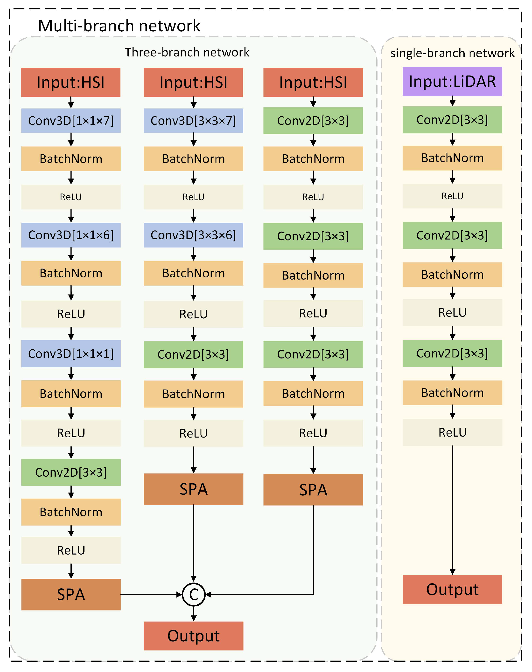
(1) Effectiveness of ${\mathrm{PC}}^2\mathrm{A}$ module: The comparative experiment of single-source image classification after adding ${\mathrm{PC}}^2\mathrm{A}$ module to LiDAR image and HSI is listed. HSI means feature extraction and classification of HSI through the multiscale network, LiDAR means feature extraction and classification of LiDAR images through the single-branch network. LiDAR-${\mathrm{PC}}^2\mathrm{A}$ means that LiDAR image adds the position-channel collaborative attention module, and HSI-${\mathrm{PC}}^2\mathrm{A}$ means that HSI adds the position-channel collaborative attention module. In order to ensure the authenticity and effectiveness of the comparative experiment, the standard data set is adopted uniformly, and all the training and test samples are the same.

Table 3. Influence of ${\mathrm{PC}}^2\mathrm{A}$ on the Houston and Trento dataset.

Dataset	Metrices	LiDAR	LiDAR-${\mathbf{PC}}^2$A	HSI	HSI-${\mathbf{PC}}^2$A	${\mathbf{PC}}^2$ ANet
2012 Houston	OA(%)	58.25	60.87	91.94	92.43	95.02
	AA(%)	61.53	62.40	92.50	93.08	94.97
	Kappa	54.94	57.69	91.25	91.78	94.59
Trento	OA(%)	87.00	87.19	96.72	97.31	99.15
	AA(%)	78.06	81.32	95.50	95.92	98.81
	Kappa	82.85	83.16	95.63	96.41	98.87

lists the overall accuracy (OA), average accuracy (AA), and Kappa coefficient of the five models on the 2012 Houston data set and Trento data set, and the best results are shown in bold. Obviously, the classification accuracy of single-source images with ${\mathrm{PC}}^2\mathrm{A}$ module is higher than that without ${\mathrm{PC}}^2\mathrm{A}$ module. In the Houston dataset, the OA of the LiDAR-${\mathrm{PC}}^2\mathrm{A}$ model is 60.87%, that of the LiDAR model is 58.25%, and the accuracy is improved by 2.62% after adding ${\mathrm{PC}}^2\mathrm{A}$ module. The OA of the HSI-${\mathrm{PC}}^2\mathrm{A}$ model is 97.31% and that of the HSI model is 96.72% on the Trento dataset, and the accuracy is improved by 0.59% after adding ${\mathrm{PC}}^2\mathrm{A}$ module. Figure 7 shows the classification results of the five models listed in Table 3 on the Houston data set. It can be seen that from Figure 7a–e, the category classification becomes clearer and the results become more obvious. 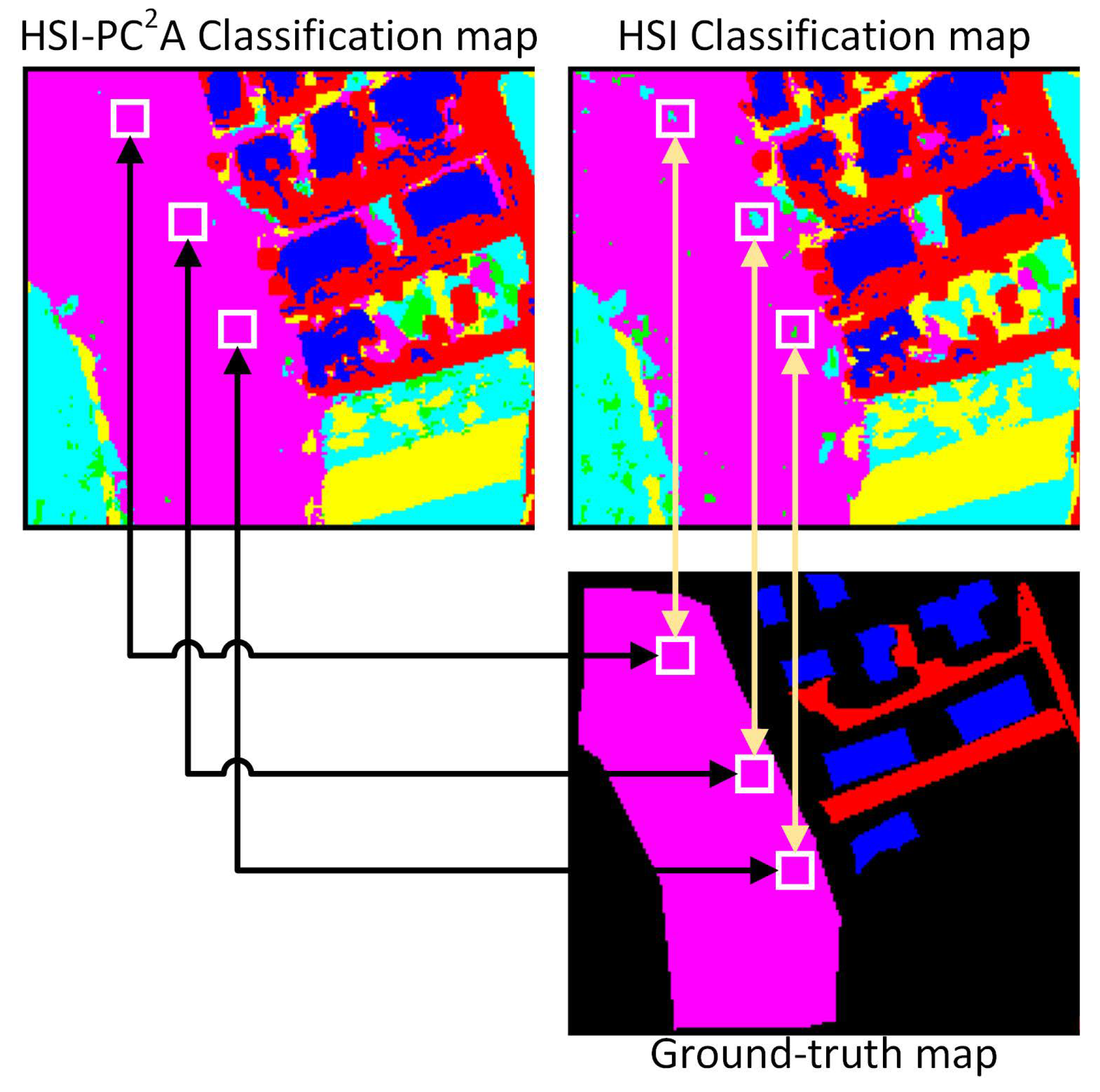Figure 8 shows the partial sorting results on the Trento data set, which is primarily used to compare the classification details of HSI and HSI-${\mathrm{PC}}^2\mathrm{A}$ models. In this partial map, the class of Wood occupies a large area, and when using the HSI model for classification, some Wood will be mistakenly classified as vineyard and apple trees. With the addition of ${\mathrm{PC}}^2\mathrm{A}$ module, the model pays more attention to the detailed information of categories and can make better identification. It can be seen from Figure 8 that the classification effect of the HSI-${\mathrm{PC}}^2\mathrm{A}$ model on the wood category is obviously better than that of the HSI model.

The result of single-source classification of LiDAR images is the worst among the methods listed in Table 3. However, LiDAR data can provide potential details for HSI, including the height and shape information of ground objects, which is a necessary supplement to HSI defects. The OA of LiDAR image and HSI after feature fusion classification is also much higher than that of HSI single source classification, which verifies the indispensability of LiDAR data and fully demonstrates the effectiveness of feature fusion.

(2) Effectiveness of the proposed ${\mathrm{PC}}^2\mathrm{ANet}$: To validate the effectiveness of the proposed method, the proposed model ${\mathrm{PC}}^2\mathrm{ANet}$ is compared with advanced deep learning models such as Two-Branch CNN [40], EndNet [41], MDL-Middle [42], FusAtNet [49], IP-CNN [43], CRNN [4], ${\mathrm{S}}^2\mathrm{ENet}$ [50] and HRWN [37]. To make a fair comparison, all training and testing samples are the same. In which, two-branch CNN realizes feature fusion by combining the spatial and spectral features extracted from HSI with LiDAR image features extracted from cascade networks. EndNet is a deep encoder–decoder network architecture, which fuses multi-modal information by strengthening fusion features. MDL-Middle is a baseline CNN model through intermediate fusion. FusAtNet is a method that generates an attention map through “self-attention” mechanism to highlight its own spectral features and highlights spatial features through “cross-attention” mechanism to realize classification. IP-CNN designed a bidirectional automatic encoder to reconstruct HSI and LiDAR data, and the reconstruction process does not depend on the labeling information. The convolutional recurrent neural network (CRNN) was proposed to learn more discriminant features in HSI data classification. ${\mathrm{S}}^2\mathrm{ENet}$ enhances the spectral and spatial representation of images through the spatial–spectral enhancement module of cross-modal information interaction to achieve the purpose of feature fusion. HRWN jointly optimizes the dual-tunnel CNN and pixel-level affinity through a random walk layer, which strengthens the spatial consistency in the deeper layer of the network.

Table 4. Classification accuracies (%) and kappa coefficients of different model on the 2012 Houston dataset.

Class	Two-Branch	EndNet	MDL-Middle	FusAtNet	IP-CNN	CRNN	${\mathbf{S}}^2$ENet	HRWN	${\mathbf{PC}}^2$ANet
C1	83.10	81.58	83.10	83.10	85.77	83.00	82.91	85.61	86.89
C2	84.10	83.65	85.06	96.05	87.34	79.41	100	85.17	99.72
C3	100	100	99.60	100	100	99.80	100	99.57	99.80
C4	93.09	93.09	91.57	93.09	94.26	90.15	96.88	92.20	97.92
C5	100	99.91	98.86	99.43	98.42	99.71	99.91	100	98.39
C6	99.30	95.10	100	100	99.91	83.21	100	98.15	95.80
C7	92.82	82.65	96.64	93.53	94.59	88.06	95.15	95.98	97.48
C8	82.34	81.29	88.13	92.12	91.81	88.61	93.92	97.59	95.06
C9	84.70	88.29	85.93	83.63	89.35	66.01	91.31	88.66	91.78
C10	65.44	89.00	74.42	64.09	72.43	52.22	92.95	86.23	98.26
C11	88.24	83.78	84.54	90.13	96.57	81.97	94.69	97.98	95.35
C12	89.53	90.39	95.39	91.93	95.60	69.83	89.43	97.40	87.22
C13	92.28	82.46	87.37	88.42	94.37	79.64	83.16	91.47	81.40
C14	96.76	100	95.14	100	99.86	100	100	100	99.60
C15	99.79	98.10	100	99.15	99.99	100	100	100	99.79
OA	87.98	88.52	89.55	89.98	92.06	88.55	94.19	93.61	95.02
AA	90.11	89.95	91.05	94.65	93.35	90.30	94.69	94.40	94.97
Kappa	86.98	87.59	88.71	89.13	91.42	87.56	93.69	93.09	94.59

and

Table 5. Classification accuracies (%) and kappa coefficients of different model on the Trento dataset.

Class	Two-Branch	EndNet	MDL-Middle	FusAtNet	IP-CNN	CRNN	${\mathbf{S}}^2$ENet	HRWN	${\mathbf{PC}}^2$ANet
C1	99.78	88.19	99.50	99.54	99.00	98.39	99.65	99.75	99.75
C2	97.93	98.49	97.55	98.49	99.40	90.46	97.31	94.32	98.28
C3	99.93	95.19	99.10	99.73	99.10	99.79	99.67	98.75	100
C4	99.46	99.30	99.90	100	99.92	96.96	99.97	100	99.90
C5	98.96	91.96	99.71	99.90	99.66	100	99.72	100	99.65
C6	91.68	90.14	92.25	93.32	90.21	81.63	93.24	94.90	95.27
OA	98.36	94.17	98.73	99.06	98.58	97.30	98.87	98.86	99.15
AA	97.96	93.88	98.00	98.50	97.88	94.54	98.26	97.95	98.81
Kappa	97.83	92.22	98.32	98.75	98.17	96.39	98.50	98.48	98.87

, respectively, list the OA, AA, and Kappa coefficient of the 2012 Houston data set and Trento data set, the precision of each class is also listed, among which the best results are shown in bold. Obviously, the experimental results of ${\mathrm{PC}}^2\mathrm{ANet}$ are better than those of other methods. Taking the 2012 Houston data set as an example, the OA of the proposed ${\mathrm{PC}}^2\mathrm{ANet}$ method is 95.02%, AA is 94.97% and Kappa is 94.59, which is the best among the listed methods. Specifically, using the Houston dataset for evaluation, it shows approximately 7.04%, 6.50%, 5.47%, 5.04%, 2.96%, 6.47%, 0.83%, and 1.41% improvements over Two-branch, EndNet, MDL-Middle, FusAtNet, IP-CNN, CRNN, ${\mathrm{S}}^2\mathrm{ENet}$, and HRWN, respectively. For the Trento data set, the categorization effect of the ${\mathrm{PC}}^2\mathrm{ANet}$ model for the two categories of Ground and Roads are significantly higher than other models. Although the classification accuracy of different models on this data set has reached a relatively high level, the taxonomy effect for the two categories Ground and Roads is less than ideal. As can be seen from Table 2, the number of samples in the categories Ground and Roads is relatively small. Due to the imbalance of sample categories, the classification results of the first category are better than that of the last category. However, the presented ${\mathrm{PC}}^2\mathrm{ANet}$ model concentrates on the detailed information of categories through the attention mechanism and learns the difference of various categories accurately for precise classification, which indicates the superiority of this model.

In terms of single category classification effect, the model ${\mathrm{PC}}^2\mathrm{ANet}$ proposed in this paper has the best classification results in the categories of healthy grass, tree, residential, commercial, road, and highway. Especially in the case of poor classification effect of healthy grass, commercial and highway, our model can show a better classification effect, which is greatly improved compared with other models.

In order to qualitatively evaluate the classification performance, Figure 9 and Figure 10 show the classification results of different methods, and the visual results are consistent with the data results in Table 4 and Table 5. The classification result of EndNet is shown in Figure 9b has more detailed information, but the OA, AA, and Kappa are far lower than that of the proposed method ${\mathrm{PC}}^2\mathrm{ANet}$. Because the input of EndNet is pixel by pixel, not pixel block, which makes the classified figures show more details. However, the correlation of adjacent pixels is not fully utilized, and only the current pixel category is considered, so the detailed information displayed by the classification results is probably wrong, which limits the classification accuracy of this model. It further demonstrates the significance of considering neighborhood information.

(3) Training and testing time cost analysis:

Table 6. Training and testing time (seconds) cost compared to models for single-source classification.

Dataset		LiDAR	LiDAR-${\mathbf{PC}}^2\mathbf{A}$	HSI	HSI-${\mathbf{PC}}^2\mathbf{A}$	${\mathbf{PC}}^2$ANet
2012 Houston	Training	258.170	340.615	298.096	319.132	425.508
	Testing	51.961	55.274	42.889	45.692	74.110
Trento	Training	185.421	201.816	273.243	294.228	357.661
	Testing	6.380	5.076	8.275	11.610	14.179

and

Table 7. Training and testing time (seconds) cost compared to advanced deep learning models.

Dataset		Two-Branch	EndNet	MDL-Middle	FusAtNet	${\mathbf{S}}^2$ENet	${\mathbf{PC}}^2$ANet
2012 Houston	Training	264.457	271.866	309.839	2519.060	338.179	425.508
	Testing	46.069	55.760	61.088	931.675	52.818	74.110
Trento	Training	139.393	121.245	145.861	882.266	190.702	357.661
	Testing	3.010	3.276	3.690	66.078	5.261	14.179

show the training and testing time cost of different models. All experiments are implemented under the same software configuration. The training process takes a long time, while the testing process takes a short time. Table 6 presents the training and testing times for the unfused model and the fused model. Obviously, the time cost of LiDAR-${\mathrm{PC}}^2\mathrm{A}$ is greater than that of LiDAR, and that of HSI-${\mathrm{PC}}^2\mathrm{A}$ is greater than that of HSI, which shows that the attention mechanism will increase the computational cost of the network, but at the same time it will improve the performance of the network. In Table 7, the training and testing time of EndNet on both datasets is short, because the neighborhood information is not considered in EndNet during training and testing. Using a single pixel as the input can save training and testing time, but ignoring the neighborhood information leads to a drop in accuracy. The training and testing times of FusAtNet, ${\mathrm{S}}^2\mathrm{ENet}$, and ${\mathrm{PC}}^2\mathrm{ANet}$ networks are relatively high. The common point of these networks is that the attention module is added, which increases the computational cost of the model, but at the same time improves the classification performance. As can be seen from Table 7, the training and testing time of the FusAtNet model is much longer than that of other models, because the model uses multiple cross-attentions, and the network is deeper than others, which extremely increases the calculation cost.

3.4. Ablation Studies

As the proposed model ${\mathrm{PC}}^2\mathrm{ANet}$ includes two modules to improve classification performance, namely, the ${\mathrm{PC}}^2\mathrm{A}$ module and the decision fusion module, in order to verify the effectiveness of these three modules, respectively, a series of ablation experiments were conducted on the 2012 Houston data set and Trento data set. Specifically, while keeping other parts of the model unchanged, the experiment was conducted in two cases: With/Without ${\mathrm{PC}}^2\mathrm{A}$ Module, and With/Without Decision Fusion, and the experimental data were compared.

(1) With/Without ${\mathrm{PC}}^2\mathrm{A}$ Module: ${\mathrm{PC}}^2\mathrm{A}$ module consists of SPA, FCA, and FPA. By weighting the position and channel features to different degrees, the extracted features contain more effective information, which is beneficial to classification, thus improving the expression ability of the model. In order to analyze the effectiveness of the ${\mathrm{PC}}^2\mathrm{A}$ module,

Table 8. Influence of with/without ${\mathrm{PC}}^2\mathrm{A}$ module on classification accuracies.

Dataset	${\mathbf{PC}}^2\mathbf{A}$ Module	OA	AA	Kappa
Houston	×	94.09	94.71	93.58
	√	95.02	94.97	94.59
Trento	×	98.85	98.35	98.47
	√	99.15	98.81	98.87

shows the results with and without the ${\mathrm{PC}}^2\mathrm{A}$ module. It is obvious that the OA, AA, and Kappa of the model with ${\mathrm{PC}}^2\mathrm{A}$ are higher than those without ${\mathrm{PC}}^2\mathrm{A}$.

Part of the categories of OA are shown in Figure 11. In the 2012 Houston data set, the classification results of most categories by this model are higher than those of other models, especially those with plenty of samples, which shows that the model has a strong learning ability. Under the condition of enough samples, it can learn the detailed information of different categories effectively, thus making accurate classification. As can be seen from Figure 11, the accuracy of most categories is improved after adding the module ${\mathrm{PC}}^2\mathrm{A}$, which proves the superiority of this module.

(2) With/Without Decision Fusion: The decision fusion (DS) module fuses the output of the HSI feature extraction network, LiDAR image feature extraction network, and the result after feature fusion. The three classification results obtained by the classification module are fused. Through the automatic learning of the network, the weight coefficient is constantly updated to obtain the optimal weight addition result. To analyze the effectiveness of the decision fusion module,

Table 9. Influence of with/without Decision Fusion on classification accuracies.

Dataset	Decision Fusion	OA	AA	Kappa
Houston	×	94.33	94.88	93.84
	√	95.02	94.97	94.59
Trento	×	98.87	98.42	98.50
	√	99.15	98.81	98.87

shows the results with and without the decision fusion module (DS). It is obvious that the OA, AA, and Kappa of the model with DS are higher than those without DS.

Figure 12 shows OA for part classes. In the 2012 Houston data set, there are nine classes of OA that are higher than those without DS. In the Trento data set, the classification results of each class are higher than those without DS. Experiments can effectively prove that the decision fusion module can obviously improve the performance of the model.

4. Conclusions

This paper proposed a position-channel cooperative attention network for HSI and LiDAR data fusion. In the feature extraction stage, HSI features are initially extracted by a multiscale network, and then the spatial information of HSI features is enhanced by the SPA module; LiDAR features are initially extracted by a single-branch network, and then the extracted HSI and LiDAR features are enhanced by FPA and FCA modules, respectively, for complementary spatial features and channel features so that the important features of the image can be paid more attention, while the attention to useless information is reduced. Feature fusion is the fusion of extracted HSI and LiDAR features through feature concatenation. After feature fusion, HSI and LiDAR features extracted by ${\mathrm{PC}}^2\mathrm{A}$ module are sent to the classification module, respectively, three different output results are combined by weighted summation, and the weights are automatically learned through network. In order to validate the effectiveness of the proposed model, we constructed experiments on two data sets. Experiments show that the proposed model is effective by comparing the qualitative and quantitative results of the 2012 Houston data and Trento data. In addition, we evaluated the influence of neighborhood size, ${\mathrm{PC}}^2\mathrm{A}$ module, and decision fusion module on classification performance through ablation experiments. Experiments show that the proposed modules and parameter settings can improve the experimental performance. In the future, we need to explore more powerful feature extraction methods and more effective feature fusion methods.

References

1. Hong, D.; Yokoya, N.; Chanussot, J.; Zhu, X.X. CoSpace: Common subspace learning from hyperspectral-multispectral correspondences. IEEE Trans. Geosci. Remote Sens. 2019, 57, 4349–4359. [Google Scholar] [CrossRef] [Green Version]
2. Lu, Z.; Xu, B.; Sun, L.; Zhan, T.; Tang, S. 3-D Channel and spatial attention based multiscale spatial–spectral residual network for hyperspectral image classification. IEEE J. Sel. Top. Appl. Earth Obs. Remote Sens. 2020, 13, 4311–4324. [Google Scholar] [CrossRef]
3. Yue, J.; Fang, L.; Rahmani, H.; Ghamisi, P. Self-supervised learning with adaptive distillation for hyperspectral image classification. IEEE Trans. Geosci. Remote Sens. 2021, 60, 1–13. [Google Scholar] [CrossRef]
4. Wu, H.; Prasad, S. Convolutional recurrent neural networks forhyperspectral data classification. Remote Sens. 2017, 9, 298. [Google Scholar] [CrossRef] [Green Version]
5. Ghamisi, P.; Benediktsson, J.A.; Sveinsson, J.R. Automatic Spectral–Spatial Classification Framework Based on Attribute Profiles and Supervised Feature Extraction. IEEE Trans. Geosci. Remote Sens. 2014, 52, 5771–5782. [Google Scholar] [CrossRef]
6. Kuras, A.; Brell, M.; Rizzi, J.; Burud, I. Hyperspectral and Lidar Data Applied to the Urban Land Cover Machine Learning and Neural-Network-Based Classification: A Review. Remote Sens. 2021, 13, 3393. [Google Scholar] [CrossRef]
7. Mäyrä, J.; Keski-Saari, S.; Kivinen, S.; Tanhuanpää, T.; Hurskainen, P.; Kullberg, P.; Poikolainen, L.; Viinikka, A.; Tuominen, S.; Kumpula, T.; et al. Tree species classification from airborne hyperspectral and LiDAR data using 3D convolutional neural networks. Remote Sens. Environ. 2021, 256, 112322. [Google Scholar] [CrossRef]
8. Wang, X.; Feng, Y.; Song, R.; Mu, Z.; Song, C. Multi-attentive hierarchical dense fusion net for fusion classification of hyperspectral and LiDAR data. Inf. Fusion 2022, 82, 1–18. [Google Scholar] [CrossRef]
9. Ghamisi, P.; Rasti, B.; Yokoya, N.; Wang, Q.; Hofle, B.; Bruzzone, L.; Bovolo, F.; Chi, M.; Anders, K.; Gloaguen, R.; et al. Multisource and multitemporal data fusion in remote sensing: A comprehensive review of the state of the art. IEEE Geosci. Remote Sens. Mag. 2019, 7, 6–39. [Google Scholar] [CrossRef] [Green Version]
10. Debes, C.; Merentitis, A.; Heremans, R.; Hahn, J.; Frangiadakis, N.; van Kasteren, T.; Liao, W.; Bellens, R.; Pižurica, A.; Gautama, S.; et al. Hyperspectral and LiDAR data fusion: Outcome of the 2013 GRSS data fusion contest. IEEE J. Sel. Top. Appl. Earth Obs. Remote Sens. 2014, 7, 2405–2418. [Google Scholar] [CrossRef]
11. Geng, J.; Deng, X.; Ma, X.; Jiang, W. Transfer Learning for SAR Image Classification Via Deep Joint Distribution Adaptation Networks. IEEE Trans. Geosci. Remote. Sens. 2020, 58, 5377–5392. [Google Scholar] [CrossRef]
12. Wang, Y.; Duan, H. Classification of Hyperspectral Images by SVM Using a Composite Kernel by Employing Spectral, Spatial and Hierarchical Structure Information. Remote Sens. 2018, 10, 26. [Google Scholar] [CrossRef] [Green Version]
13. Huang, G.B.; Zhu, Q.Y.; Siew, C.K. Extreme learning machine: Theory and applications. Neurocomputing 2006, 70, 489–501. [Google Scholar] [CrossRef]
14. Zhang, S.; Li, S.; Fu, W.; Fang, L. Multiscale superpixel-based sparse representation for hyperspectral image classification. Remote Sens. 2017, 9, 139. [Google Scholar] [CrossRef] [Green Version]
15. Hänsch, R.; Hellwich, O. Feature-independent classification of hyperspectral images by projection-based random forests. In Proceedings of the 2015 7th Workshop on Hyperspectral Image and Signal Processing: Evolution in Remote Sensing (WHISPERS), Tokyo, Japan, 2–5 June 2015; pp. 1–4. [Google Scholar]
16. Jiang, W. A correlation coefficient for belief functions. Int. J. Approx. Reason. 2018, 103, 94–106. [Google Scholar] [CrossRef] [Green Version]
17. Liu, Y.; Liu, L.; Gao, Y.; Yang, L. An Improved Random Forest Algorithm Based on Attribute Compatibility. In Proceedings of the 2019 IEEE 3rd Information Technology, Networking, Electronic and Automation Control Conference (ITNEC), Chengdu, China, 15–17 March 2019. [Google Scholar]
18. Jiang, W.; Cao, Y.; Deng, X. A Novel Z-network Model Based on Bayesian Network and Z-number. IEEE Trans. Fuzzy Syst. 2020, 28, 1585–1599. [Google Scholar] [CrossRef]
19. He, Z.; Jiang, W. An evidential Markov decision making model. Inf. Sci. 2018, 467, 357–372. [Google Scholar] [CrossRef] [Green Version]
20. Jiang, W.; Xie, C.; Zhuang, M.; Tang, Y. Failure Mode and Effects Analysis based on a novel fuzzy evidential method. Appl. Soft Comput. 2017, 57, 672–683. [Google Scholar] [CrossRef]
21. Pedergnana, M.; Marpu, P.R.; Dalla Mura, M.; Benediktsson, J.A.; Bruzzone, L. Classification of remote sensing optical and LiDAR data using extended attribute profiles. IEEE J. Sel. Top. Signal Process. 2012, 6, 856–865. [Google Scholar] [CrossRef]
22. Gu, Y.; Wang, Q.; Jia, X.; Benediktsson, J.A. A novel MKL model of integrating LiDAR data and MSI for urban area classification. IEEE Trans. Geosci. Remote Sens. 2015, 53, 5312–5326. [Google Scholar]
23. Ge, C.; Du, Q.; Li, W.; Li, Y.; Sun, W. Hyperspectral and LiDAR data classification using kernel collaborative representation based residual fusion. IEEE J. Sel. Top. Appl. Earth Obs. Remote Sens. 2019, 12, 1963–1973. [Google Scholar] [CrossRef]
24. Tong, Y.; Quan, Y.; Feng, W.; Dauphin, G.; Wang, Y.; Wu, P.; Xing, M. Multi-Scale Feature Extraction and Total Variation Based Fusion Method For HSI and Lidar Data Classification. In Proceedings of the 2021 IEEE International Geoscience and Remote Sensing Symposium IGARSS, Brussels, Belgium, 11–16 July 2021; pp. 5433–5436. [Google Scholar]
25. Jia, S.; Zhan, Z.; Xu, M. Shearlet-Based Structure-Aware Filtering for Hyperspectral and LiDAR Data Classification. J. Remote Sens. 2021, 2021, 9825415. [Google Scholar] [CrossRef]
26. Huang, K.; Geng, J.; Jiang, W.; Deng, X.; Xu, Z. Pseudo-Loss Confidence Metric for Semi-Supervised Few-Shot Learning. In Proceedings of the IEEE/CVF International Conference on Computer Vision, Montreal, BC, Canada, 11–17 October 2021; pp. 8671–8680. [Google Scholar]
27. Xu, K.; Huang, H.; Deng, P.; Li, Y. Deep feature aggregation framework driven by graph convolutional network for scene classification in remote sensing. IEEE Trans. Neural Netw. Learn. Syst. 2021. [Google Scholar] [CrossRef] [PubMed]
28. He, Z.; Jiang, W. An evidential dynamical model to predict the interference effect of categorization on decision making. Knowl.-Based Syst. 2018, 150, 139–149. [Google Scholar] [CrossRef]
29. Jiang, W.; Huang, K.; Geng, J.; Deng, X. Multi-Scale Metric Learning for Few-Shot Learning. IEEE Trans. Circuits Syst. Video Technol. 2021, 31, 1091–1102. [Google Scholar] [CrossRef]
30. He, Q.; Sun, X.; Yan, Z.; Fu, K. DABNet: Deformable contextual and boundary-weighted network for cloud detection in remote sensing images. IEEE Trans. Geosci. Remote. Sens. 2021, 60, 1–16. [Google Scholar] [CrossRef]
31. Sun, Y.; Fu, Z.; Sun, C.; Hu, Y.; Zhang, S. Deep Multimodal Fusion Network for Semantic Segmentation Using Remote Sensing Image and LiDAR Data. IEEE Trans. Geosci. Remote Sens. 2021, 60. [Google Scholar] [CrossRef]
32. Bazi, Y.; Bashmal, L.; Rahhal, M.M.A.; Dayil, R.A.; Ajlan, N.A. Vision transformers for remote sensing image classification. Remote Sens. 2021, 13, 516. [Google Scholar] [CrossRef]
33. Miao, W.; Geng, J.; Jiang, W. Semi-Supervised Remote Sensing Image Scene Classification Using Representation Consistency Siamese Network. IEEE Trans. Geosci. Remote Sens. 2022, 60. [Google Scholar] [CrossRef]
34. Li, H.; Ghamisi, P.; Soergel, U.; Zhu, X.X. Hyperspectral and LiDAR fusion using deep three-stream convolutional neural networks. Remote Sens. 2018, 10, 1649. [Google Scholar] [CrossRef] [Green Version]
35. Zhao, C.; Gao, X.; Wang, Y.; Li, J. Efficient multiple-feature learning-based hyperspectral image classification with limited training samples. IEEE Trans. Geosci. Remote Sens. 2016, 54, 4052–4062. [Google Scholar] [CrossRef]
36. Hang, R.; Li, Z.; Ghamisi, P.; Hong, D.; Xia, G.; Liu, Q. Classification of hyperspectral and LiDAR data using coupled CNNs. IEEE Trans. Geosci. Remote Sens. 2020, 58, 4939–4950. [Google Scholar] [CrossRef] [Green Version]
37. Zhao, X.; Tao, R.; Li, W.; Li, H.C.; Du, Q.; Liao, W.; Philips, W. Joint classification of hyperspectral and LiDAR data using hierarchical random walk and deep CNN architecture. IEEE Trans. Geosci. Remote Sens. 2020, 58, 7355–7370. [Google Scholar] [CrossRef]
38. Zhang, M.; Li, W.; Du, Q.; Gao, L.; Zhang, B. Feature extraction for classification of hyperspectral and LiDAR data using patch-to-patch CNN. IEEE Trans. Cybern. 2018, 50, 100–111. [Google Scholar] [CrossRef] [PubMed]
39. Hong, D.; Yokoya, N.; Xia, G.S.; Chanussot, J.; Zhu, X.X. X-ModalNet: A semi-supervised deep cross-modal network for classification of remote sensing data. ISPRS J. Photogramm. Remote Sens. 2020, 167, 12–23. [Google Scholar] [CrossRef] [PubMed]
40. Xu, X.; Li, W.; Ran, Q.; Du, Q.; Gao, L.; Zhang, B. Multisource remote sensing data classification based on convolutional neural network. IEEE Trans. Geosci. Remote Sens. 2017, 56, 937–949. [Google Scholar] [CrossRef]
41. Hong, D.; Gao, L.; Hang, R.; Zhang, B.; Chanussot, J. Deep Encoder–Decoder Networks for Classification of Hyperspectral and LiDAR Data. IEEE Geosci. Remote Sens. Lett. 2022, 19, 1–5. [Google Scholar] [CrossRef]
42. Hong, D.; Gao, L.; Yokoya, N.; Yao, J.; Chanussot, J.; Du, Q.; Zhang, B. More Diverse Means Better: Multimodal Deep Learning Meets Remote-Sensing Imagery Classification. IEEE Trans. Geosci. Remote Sens. 2021, 59, 4340–4354. [Google Scholar] [CrossRef]
43. Zhang, M.; Li, W.; Tao, R.; Li, H.; Du, Q. Information fusion for classification of hyperspectral and LiDAR data using IP-CNN. IEEE Trans. Geosci. Remote Sens. 2021, 60, 1–12. [Google Scholar] [CrossRef]
44. Vaswani, A.; Shazeer, N.; Parmar, N.; Uszkoreit, J.; Jones, L.; Gomez, A.N.; Kaiser, L.; Polosukhin, I. Attention is All You Need. arXiv 2017, arXiv:1706.03762. [Google Scholar]
45. Hu, J.; Shen, L.; Sun, G. Squeeze-and-Excitation Networks. In Proceedings of the IEEE Conference on Computer Vision and Pattern Recognition (CVPR), Salt Lake City, UT, USA, 18–23 June 2018. [Google Scholar]
46. Woo, S.; Park, J.; Lee, J.Y.; Kweon, I.S. Cbam: Convolutional block attention module. In Proceedings of the European Conference on Computer Vision (ECCV), Munich, Germany, 8–14 September 2018; pp. 3–19. [Google Scholar]
47. Park, J.; Woo, S.; Lee, J.Y.; Kweon, I.S. A simple and light-weight attention module for convolutional neural networks. Int. J. Comput. Vis. 2020, 128, 783–798. [Google Scholar] [CrossRef]
48. Fu, J.; Liu, J.; Tian, H.; Li, Y.; Bao, Y.; Fang, Z.; Lu, H. Dual attention network for scene segmentation. In Proceedings of the IEEE/CVF Conference on Computer Vision and Pattern Recognition, Long Beach, CA, USA, 15–20 June 2019; pp. 3146–3154. [Google Scholar]
49. Mohla, S.; Pande, S.; Banerjee, B.; Chaudhuri, S. Fusatnet: Dual attention based spectrospatial multimodal fusion network for hyperspectral and lidar classification. In Proceedings of the IEEE/CVF Conference on Computer Vision and Pattern Recognition Workshops, Seattle, WA, USA, 14–19 June 2020; pp. 92–93. [Google Scholar]
50. Fang, S.; Li, K.; Li, Z. S2ENet: Spatial–Spectral Cross-Modal Enhancement Network for Classification of Hyperspectral and LiDAR Data. IEEE Geosci. Remote. Sens. Lett. 2022, 19, 1–5. [Google Scholar] [CrossRef]
Figure 1. Proposed classification framework of PC 2 ANet .
Remotesensing 14 03247 g001
Figure 2. Overall parameter configuration of the designed feature extraction model.
Remotesensing 14 03247 g002
Figure 3. Position-channel collaborative attention module. (a) SPA. (b) FPA. (c) FCA.
Remotesensing 14 03247 g003
Figure 4. Visualization of the 2012 Houston Data. (a) False-color images of hyperspectral data using 64, 43, and 22 as R, G, B, respectively. (b) Gray images of LiDAR data. (c) Ground-truth map.
Remotesensing 14 03247 g004
Figure 5. Visualization of the Trento Data. (a) False-color images of hyperspectral data using 40, 20, and 10 as R, G, B, respectively. (b) Gray images of LiDAR data. (c) Ground-truth map.
Remotesensing 14 03247 g005
Figure 6. Classification performance of the proposed PC 2 ANet with different patch scales.
Remotesensing 14 03247 g006
Figure 7. Visualization of the influence of PC 2 A module on 2012 Houston data set. (a) LiDAR. (b) LiDAR- PC 2 A . (c) HSI. (d) HSI- PC 2 A . (e) PC 2 ANet .
Remotesensing 14 03247 g007
Figure 8. Partial detail classification diagram with/without PC 2 A module on Trento dataset.
Remotesensing 14 03247 g008
Figure 9. Classification maps of the 2012 Houston data using different models. (a) Two-branch. (b) EndNet. (c) MDL-Middle. (d) FusAtNet. (e) S 2 ENet . (f) PC 2 ANet .
Remotesensing 14 03247 g009
Figure 10. Classification maps of the Trento data using different models. (a) Two-branch. (b) EndNet. (c) MDL-Middle. (d) FusAtNet. (e) S 2 ENet . (f) PC 2 ANet .
Remotesensing 14 03247 g010
Figure 11. Influence of with/without PC 2 A module on classification accuracies of each class. (a) 2012 Houston data set. (b) Trento data set.
Remotesensing 14 03247 g011
Figure 12. Influence of with/without decision fusion module on classification accuracies of each class. (a) 2012 Houston data set. (b) Trento data set.
Remotesensing 14 03247 g012