
RAMC: A Rotation Adaptive Tracker with Motion Constraint for Satellite Video Single-Object Tracking


Abstract
:1. Introduction
- (1)
- (2)
- (1)
- We analyze the relationship between the intuitive rotation and the potential translation. And the rotation and translation motion patterns are decoupled by decomposing the rotation phenomenon into a translation solution. It could achieve adaptive rotation estimation when applied to SOT in SVs.
- (2)
- The appearance and motion information, contained in adjacent frames, are then synergized into the framework. It constructs the motion constraint term on the appearance model to prevent tracking drift and guarantee precise localization.
- (3)
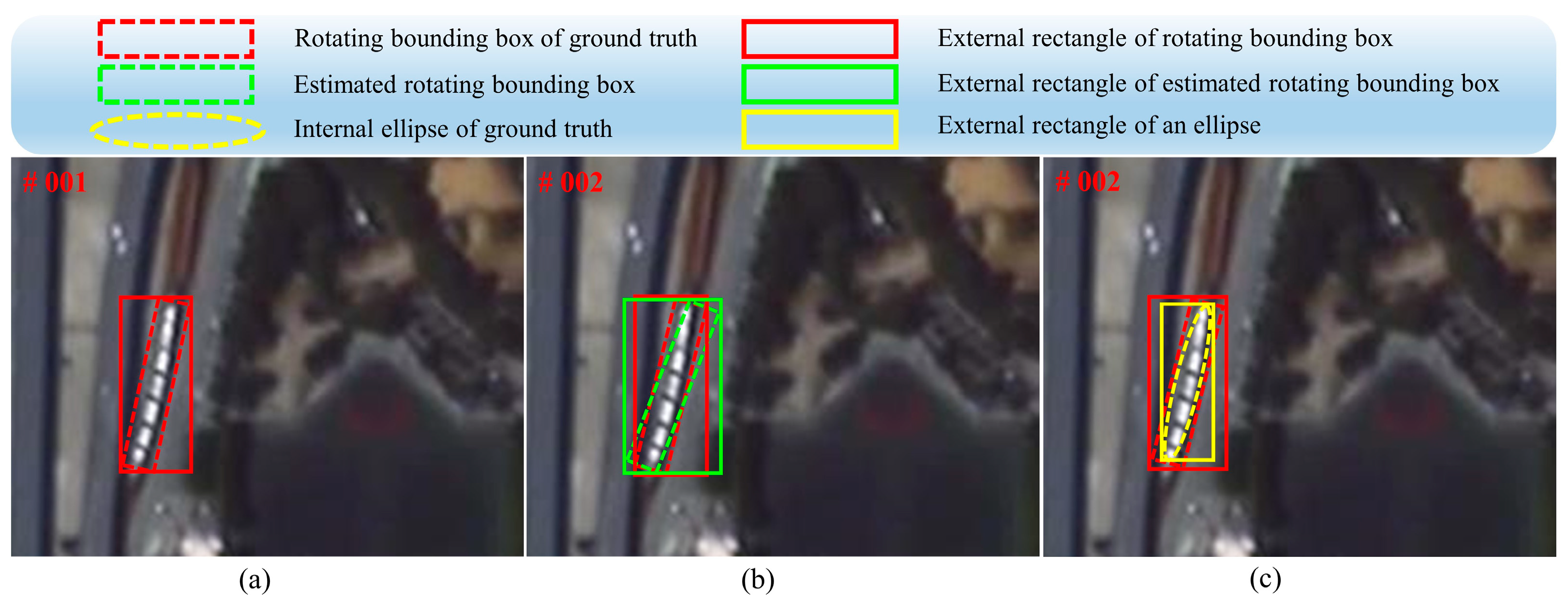
- An internal shrinkage strategy is proposed to narrow the gap between the rotating and axis-aligned bounding boxes in the evaluation benchmark. It models axis-aligned rectangles with ellipse-like distributions to optimize the evaluation process.
2. Background
2.1. Satellite Video Single-Object Tracking
2.2. Kernelized Correlation Filter
3. Methodology
3.1. Rotation Branch for Adaptive Angle Estimation
| Algorithm 1 Rotation Branch Procedure |
Input: frame index:, total frames: , image frame: , position: , rotation template: , learning rate of rotation templates: ; Output: rotation angle of the object at :; 1: for 2: if 3: /* carry out initialization in the first frame */ 4: /* set a tracked object by ) */ 5: Initialize the angle in the first frame; 6: Initialize the rotation template in the first frame; 7: else 8: Extract rotated patch at at angle from ; 9: Convert to log-polar coordinates and obtain patch ; 10: Extract HOG feature of patch ; 11: Calculate the phase correlation function between and ; 12: Estimate angle difference ; 13: Update angle ; 14: Update template ; 15: return: 16: end if 17: end for |
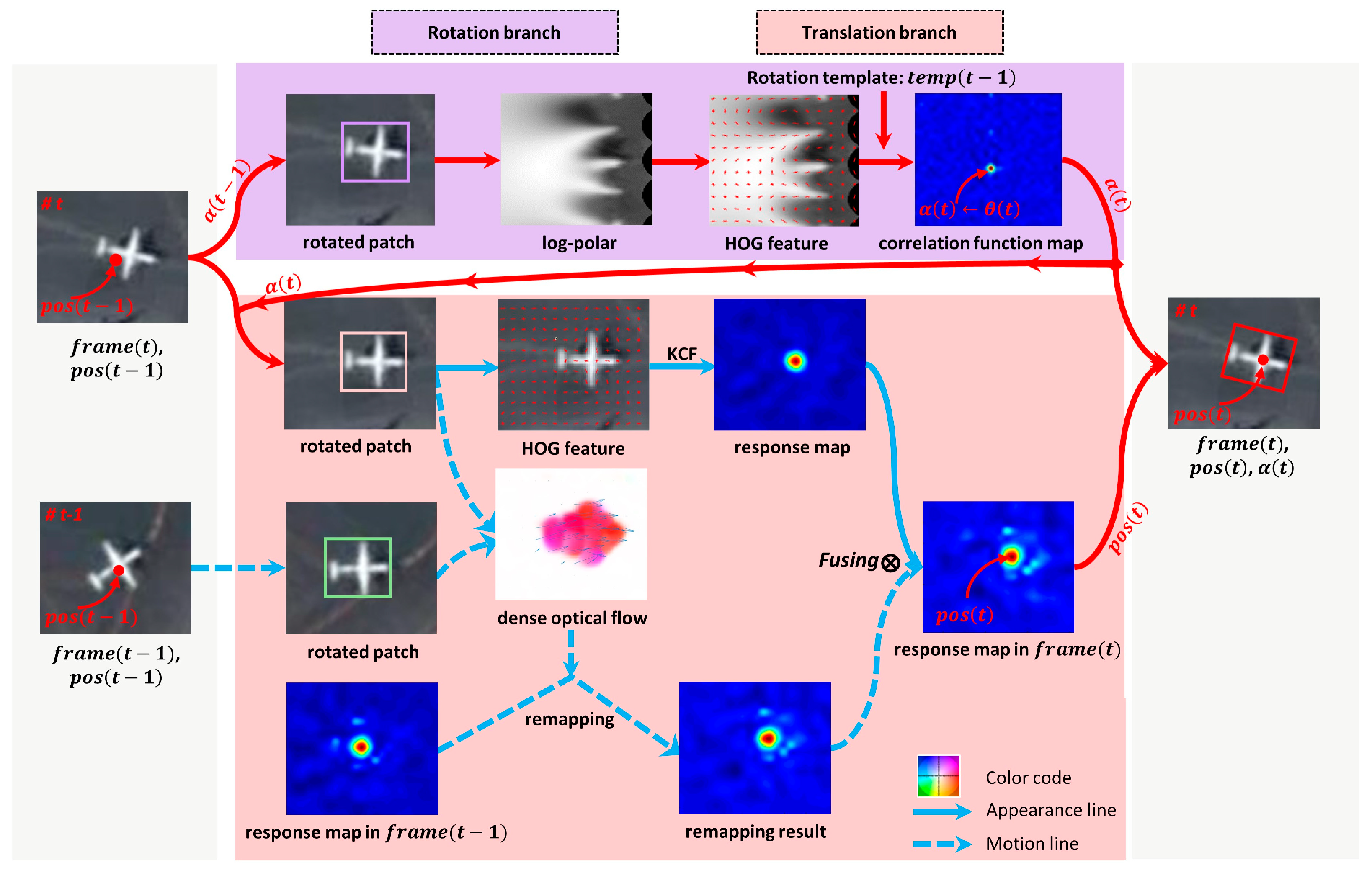
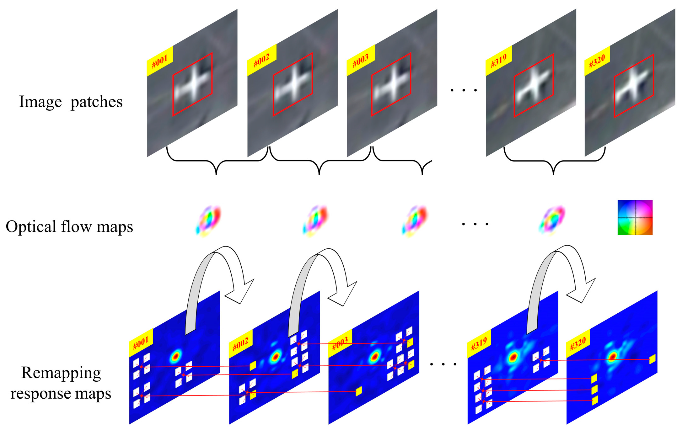
3.2. Translation Branch with Motion Constraint
4. Experimental Details and Analysis
4.1. Experimental Settings
4.1.1. Datasets
4.1.2. Evaluation Metrics
4.1.3. Implementation Details
4.2. Ablation Experiments
4.3. Comparisons on Satellite Video Datasets
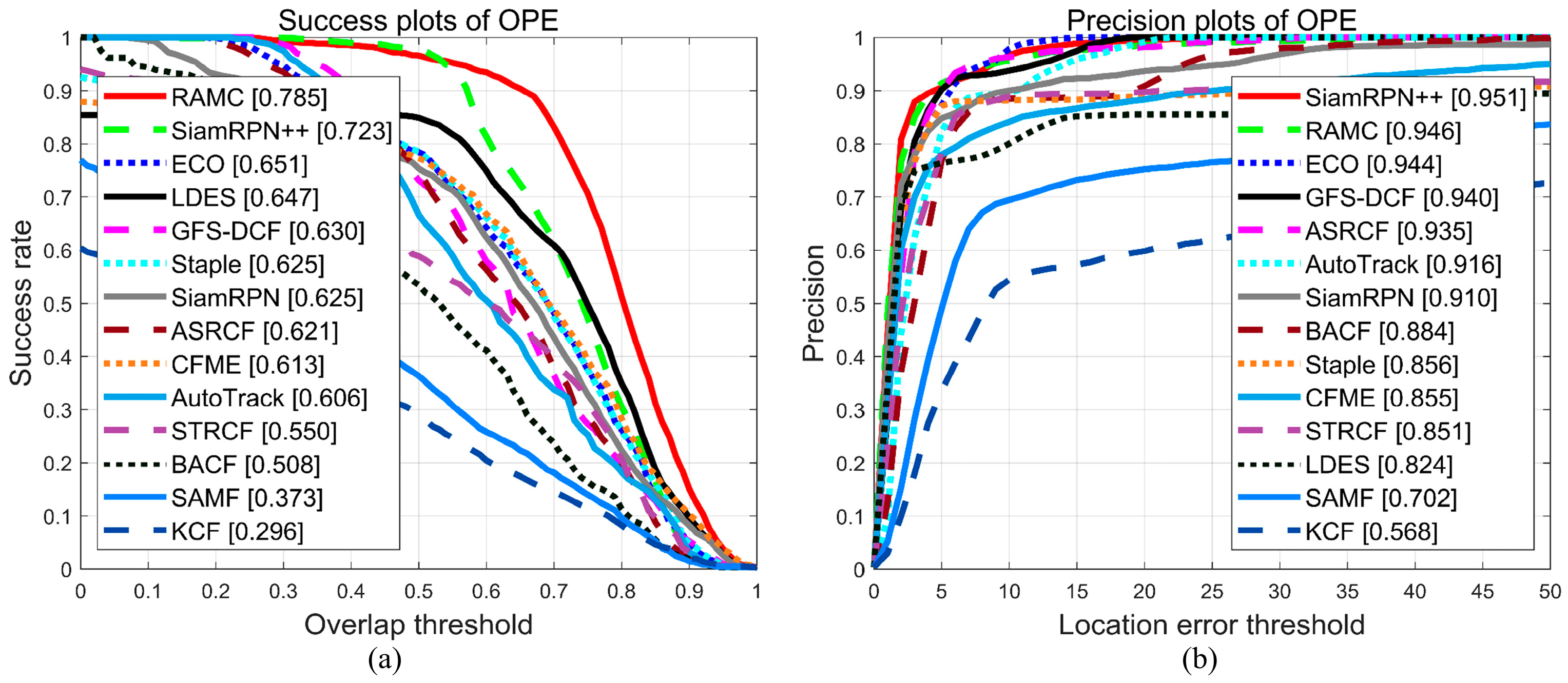
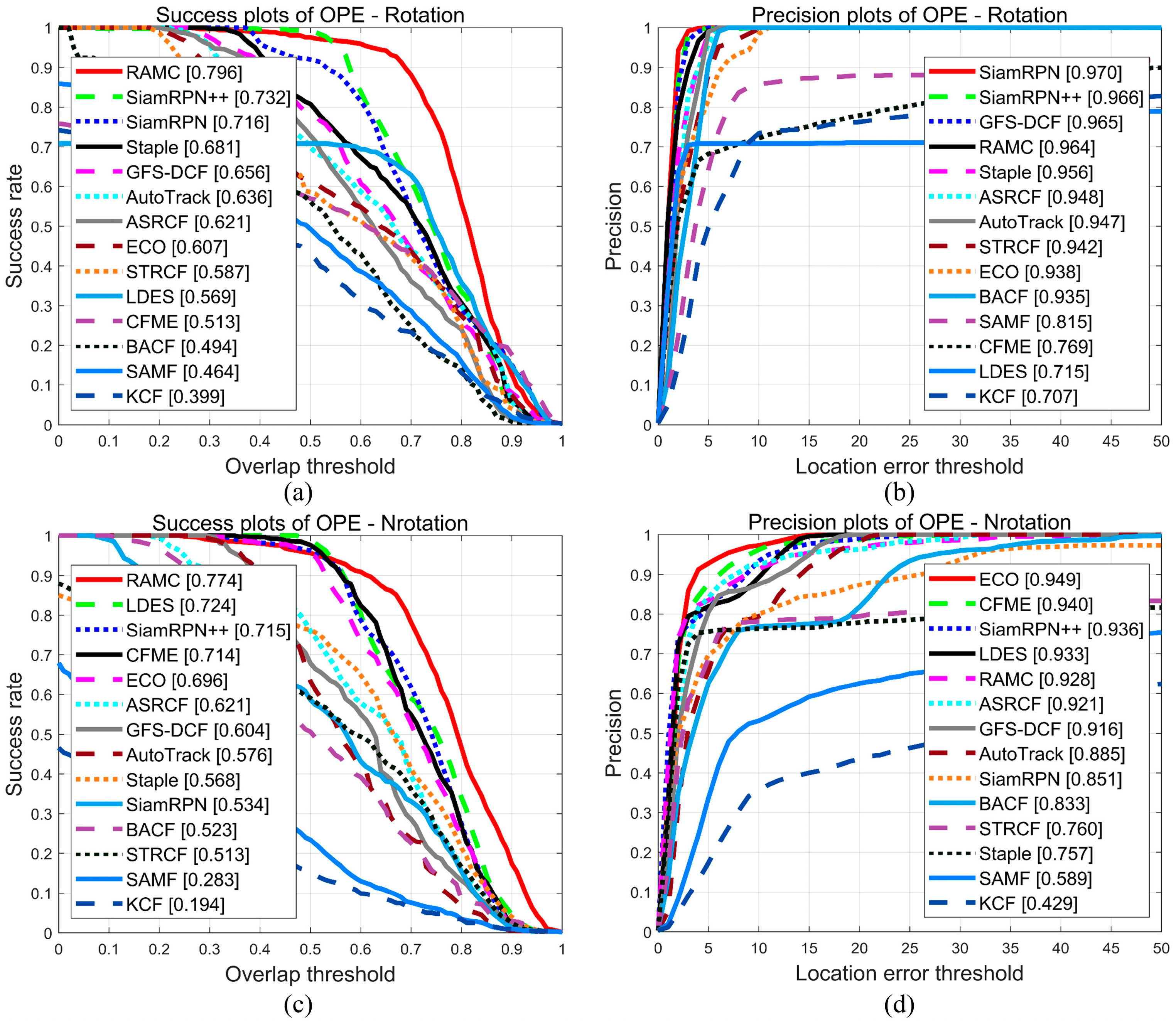
4.3.1. Quantitative Evaluation
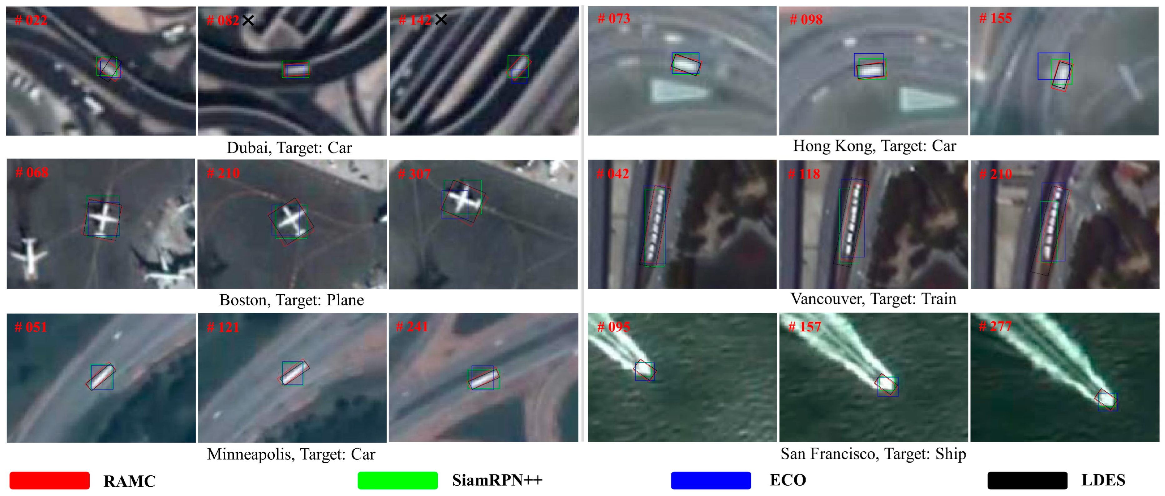
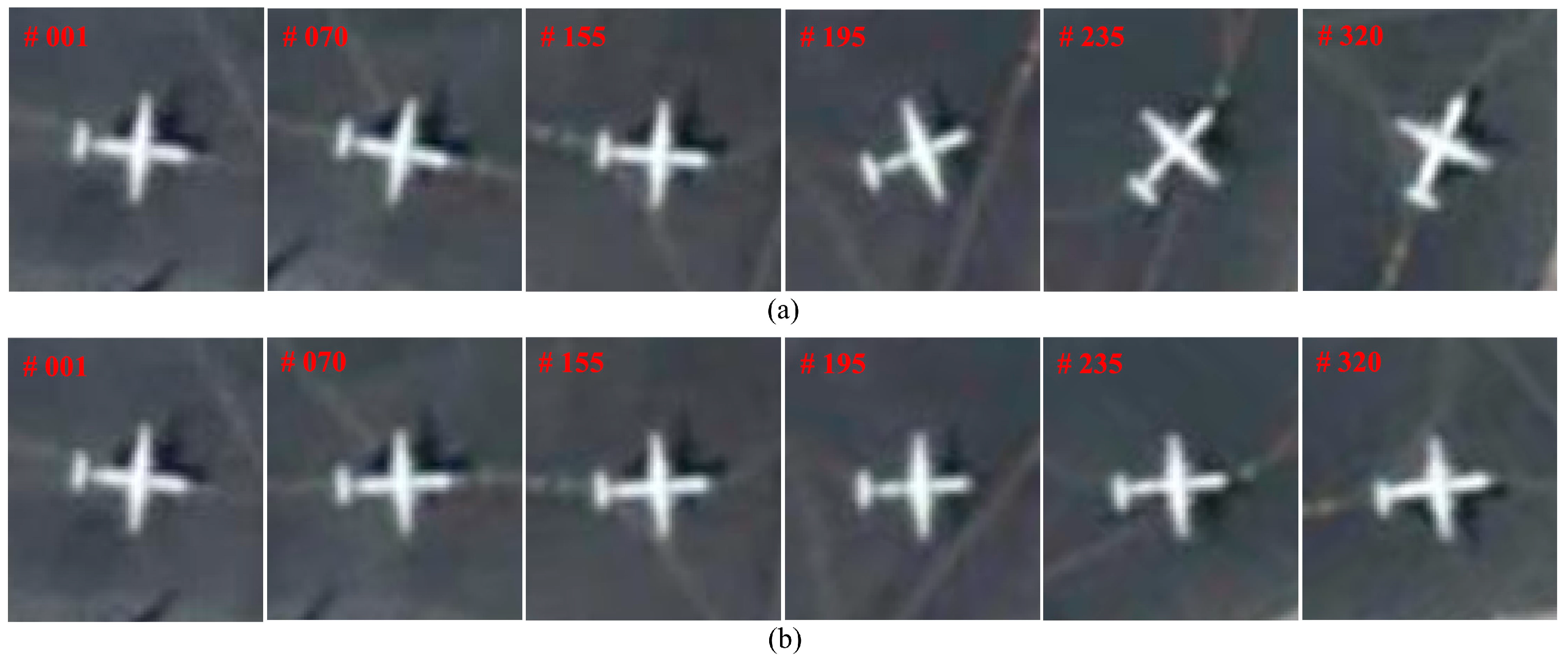
4.3.2. Qualitative Evaluation
5. Discussion
6. Conclusions
Author Contributions
Funding
Acknowledgments
Conflicts of Interest
References
- Makovski, T.; Vazquez, G.A.; Jiang, Y.V. Visual Learning in Multiple-Object Tracking. PLoS ONE 2008, 3, e2228. [Google Scholar] [CrossRef] [PubMed]
- Xing, J.; Ai, H.; Lao, S. Multiple Human Tracking Based on Multi-view Upper-Body Detection and Discriminative Learning. In Proceedings of the 20th International Conference on Pattern Recognition, Istanbul, Turkey, 23–26 August 2010; pp. 1698–1701. [Google Scholar] [CrossRef] [Green Version]
- Zhang, G.; Vela, P.A. Good Features to Track for VisuaL SLAM. In Proceedings of the IEEE Conference on Computer Vision and Pattern Recognition, Boston, MA, USA, 7–12 June 2015. [Google Scholar] [CrossRef]
- Smeulders, A.W.; Chu, D.M.; Cucchiara, R.; Calderara, S.; Dehghan, A.; Shah, M. Visual Tracking: An Experimental Survey. IEEE Trans. Pattern Anal. Mach. Intell. 2014, 36, 1442–1468. [Google Scholar] [CrossRef] [PubMed] [Green Version]
- Bertinetto, L.; Valmadre, J.; Henriques, J.F.; Vedaldi, A.; Torr, P.H.S. Fully-Convolutional Siamese Networks for Object Tracking. In European Conference on Computer Vision; Springer: Cham, Switzerland, 2016; Volume 9914, pp. 850–865. [Google Scholar] [CrossRef] [Green Version]
- Nam, H.; Han, B. Learning Multi-domain Convolutional Neural Networks for Visual Tracking. In Proceedings of the IEEE Conference on Computer Vision and Pattern Recognition, Las Vegas, NV, USA, 27–30 June 2016; pp. 4293–4302. [Google Scholar] [CrossRef] [Green Version]
- Li, B.; Yan, J.; Wu, W.; Zhu, Z.; Hu, X. High Performance Visual Tracking with Siamese Region Proposal Network. In Proceedings of the IEEE Conference on Computer Vision and Pattern Recognition, Salt Lake City, UT, USA, 18–23 June 2018; pp. 8971–8980. [Google Scholar] [CrossRef]
- Li, B.; Wu, W.; Wang, Q.; Zhang, F.; Xing, J.; Yan, J. SiamRPN++: Evolution of Siamese Visual Tracking with Very Deep Networks. In Proceedings of the IEEE Conference on Computer Vision and Pattern Recognition, Long Beach, CA, USA, 16–20 June 2019; pp. 4277–4286. [Google Scholar] [CrossRef] [Green Version]
- Chen, Z.; Zhong, B.; Li, G.; Zhang, S.; Ji, R. Siamese Box Adaptive Network for Visual Tracking. In Proceedings of the IEEE Conference on Computer Vision and Pattern Recognition, Seattle, WA, USA, 14–19 June 2020; pp. 6667–6676. [Google Scholar] [CrossRef]
- Henriques, J.F.; Caseiro, R.; Martins, P.; Batista, J. High-Speed Tracking with Kernelized Correlation Filters. IEEE Trans. Pattern Anal. Mach. Intell. 2015, 37, 583–596. [Google Scholar] [CrossRef] [PubMed] [Green Version]
- Bertinetto, L.; Valmadre, J.; Golodetz, S.; Miksik, O.; Torr, P.H.S. Staple: Complementary Learners for Real-Time Tracking. In Proceedings of the IEEE Conference on Computer Vision and Pattern Recognition, Las Vegas, NV, USA, 27–30 June 2016; pp. 1401–1409. [Google Scholar] [CrossRef] [Green Version]
- Galoogahi, H.K.; Fagg, A.; Lucey, S. Learning Background-Aware Correlation Filters for Visual Tracking. In Proceedings of the IEEE International Conference on Computer Vision, Venice, Italy, 22–29 October 2017; pp. 1144–1152. [Google Scholar] [CrossRef] [Green Version]
- Lukezic, A.; Vojir, T.; Zajc, L.C.; Matas, J.; Kristan, M. Discriminative Correlation Filter Tracker with Channel and Spatial Reliability. Int. J. Comput. Vis. 2018, 126, 671–688. [Google Scholar] [CrossRef] [Green Version]
- Hong, S.; You, T.; Kwak, S.; Han, B. Online Tracking by Learning Discriminative Saliency Map with Convolutional Neural Network. In Proceedings of the International Conference on Machine Learning, Lille, France, 7–9 July 2015; pp. 597–606. [Google Scholar] [CrossRef]
- Cortes, C.; Vapnik, V. Support Vector Networks. Mach. Learn. 1995, 20, 273–297. [Google Scholar] [CrossRef]
- Nam, H.; Baek, M.; Han, B. Modeling and Propagating CNNs in a Tree Structure for Visual Tracking. arXiv 2016, arXiv:1608.07242. [Google Scholar] [CrossRef]
- Wang, Q.; Zhang, L.; Bertinetto, L.; Hu, W.; Torr, P.H.S. Fast Online Object Tracking and Segmentation: A Unifying Approach. In Proceedings of the IEEE/CVF Conference on Computer Vision and Pattern Recognition, Long Beach, CA, USA, 16–20 June 2019; pp. 1328–1338. [Google Scholar] [CrossRef] [Green Version]
- Danelljan, M.; Hager, G.; Khan, F.S.; Felsberg, M. Convolutional Features for Correlation Filter Based Visual Tracking. In Proceedings of the IEEE International Conference on Computer Vision Workshops, Santiago, Chile, 11–18 December 2015; pp. 621–629. [Google Scholar] [CrossRef] [Green Version]
- Danelljan, M.; Robinson, A.; Khan, F.S.; Felsberg, M. Beyond Correlation Filters: Learning Continuous Convolution Operators for Visual Tracking. In Proceedings of the European Conference on Computer Vision, Amsterdam, The Netherlands, 8–16 October 2016; pp. 472–488. [Google Scholar] [CrossRef] [Green Version]
- Danelljan, M.; Bhat, G.; Khan, F.S.; Felsberg, M. ECO: Efficient Convolution Operators for Tracking. In Proceedings of the IEEE Conference on Computer Vision and Pattern Recognition, Honolulu, HI, USA, 21–26 July 2017; pp. 6931–6939. [Google Scholar] [CrossRef] [Green Version]
- Bolme, D.S.; Beveridge, J.R.; Draper, B.A.; Lui, Y.M. Visual Object Tracking using Adaptive Correlation Filters. In Proceedings of the IEEE Conference on Computer Vision and Pattern Recognition, San Francisco, CA, USA, 13–18 June 2010; pp. 2544–2550. [Google Scholar] [CrossRef]
- Henriques, J.F.; Caseiro, R.; Martins, P.; Batista, J. Exploiting the Circulant Structure of Tracking-by-Detection with Kernels. In European Conference on Computer Vision; Springer: Berlin/Heidelberg, Germany, 2012; Volume 7575, pp. 702–715. [Google Scholar] [CrossRef]
- Dalal, N.; Triggs, B. Histograms of oriented gradients for human detection. In Proceedings of the IEEE Conference on Computer Vision and Pattern Recognition, San Diego, CA, USA, 20–25 June 2005; pp. 886–893. [Google Scholar] [CrossRef] [Green Version]
- Li, Y.; Liu, G. Learning a Scale-and-Rotation Correlation Filter for Robust Visual Tracking. In Proceedings of the IEEE International Conference on Image Processing (ICIP), Phoenix, AZ, USA, 25–28 September 2016; pp. 454–458. [Google Scholar] [CrossRef]
- Rout, L.; Siddhartha; Mishra, D.; Gorthi, R. Rotation Adaptive Visual Object Tracking with Motion Consistency. In Proceedings of the 18th IEEE Winter Conference on Applications of Computer Vision (WACV), Lake Tahou, NV/CA, USA, 12–15 March 2018; pp. 1047–1055. [Google Scholar] [CrossRef] [Green Version]
- Li, Y.; Zhu, J.; Hoi, S.C.H.; Song, W.; Wang, Z.; Liu, H.; Aaai. Robust Estimation of Similarity Transformation for Visual Object Tracking. In Proceedings of the 33rd AAAI Conference on Artificial Intelligence/31st Innovative Applications of Artificial Intelligence Conference/9th AAAI Symposium on Educational Advances in Artificial Intelligence, Honolulu, HI, USA, 27 February–1 March 2019; pp. 8666–8673. [Google Scholar] [CrossRef] [Green Version]
- Danelljan, M.; Hager, G.; Khan, F.S.; Felsberg, M. Learning Spatially Regularized Correlation Filters for Visual Tracking. In Proceedings of the 2015 IEEE International Conference on Computer Vision (ICCV), Santiago, Chile, 11–18 December 2015; pp. 4310–4318. [Google Scholar] [CrossRef] [Green Version]
- Zhang, G. Satellite video processing and applications. J. Appl. Sci. 2016, 34, 361–370. [Google Scholar] [CrossRef]
- Wang, Y.M.; Wang, T.Y.; Zhang, G.; Cheng, Q.; Wu, J.Q. Small Target Tracking in Satellite Videos Using Background Compensation. IEEE Trans. Geosci. Remote Sens. 2020, 58, 7010–7021. [Google Scholar] [CrossRef]
- Shao, J.; Du, B.; Wu, C.; Gong, M.; Liu, T. HRSiam: High-Resolution Siamese Network, Towards Space-Borne Satellite Video Tracking. IEEE Trans. Image Process. 2021, 30, 3056–3068. [Google Scholar] [CrossRef]
- Zhu, K.; Zhang, X.D.; Chen, G.Z.; Tan, X.L.; Liao, P.Y.; Wu, H.Y.; Cui, X.J.; Zuo, Y.A.; Lv, Z.Y. Single Object Tracking in Satellite Videos: Deep Siamese Network Incorporating an Interframe Difference Centroid Inertia Motion Model. Remote Sens. 2021, 13, 1298. [Google Scholar] [CrossRef]
- Yin, Z.Y.; Tang, Y.Q. Analysis of Traffic Flow in Urban Area for Satellite Video. In Proceedings of the IEEE International Geoscience and Remote Sensing Symposium (IGARSS), Waikoloa, HI, USA, 26 September–2 October 2020; pp. 2898–2901. [Google Scholar] [CrossRef]
- Li, W.T.; Gao, F.; Zhang, P.; Li, Y.H.; An, Y.; Zhong, X.; Lu, Q. Research on Multiview Stereo Mapping Based on Satellite Video Images. IEEE Access 2021, 9, 44069–44083. [Google Scholar] [CrossRef]
- Legleiter, C.J.; Kinzel, P.J. Surface Flow Velocities From Space: Particle Image Velocimetry of Satellite Video of a Large, Sediment-Laden River. Front. Water 2021, 3, 652213. [Google Scholar] [CrossRef]
- Ao, W.; Fu, Y.; Hou, X.; Xu, F. Needles in a Haystack: Tracking City-Scale Moving Vehicles from Continuously Moving Satellite. IEEE Trans. Image Process. 2019, 29, 1944–1957. [Google Scholar] [CrossRef] [PubMed]
- Xuan, S.Y.; Li, S.Y.; Han, M.F.; Wan, X.; Xia, G.S. Object Tracking in Satellite Videos by Improved Correlation Filters with Motion Estimations. IEEE Trans. Geosci. Remote Sens. 2020, 58, 1074–1086. [Google Scholar] [CrossRef]
- Guo, Y.J.; Yang, D.Q.; Chen, Z.Z. Object Tracking on Satellite Videos: A Correlation Filter-Based Tracking Method with Trajectory Correction by Kalman Filter. IEEE J. Sel. Top. Appl. Earth Obs. Remote Sens. 2019, 12, 3538–3551. [Google Scholar] [CrossRef]
- Shao, J.; Du, B.; Wu, C.; Zhang, L.F. Tracking Objects from Satellite Videos: A Velocity Feature Based Correlation Filter. IEEE Trans. Geosci. Remote Sens. 2019, 57, 7860–7871. [Google Scholar] [CrossRef]
- Shao, J.; Du, B.; Wu, C.; Zhang, L. Can We Track Targets From Space? A Hybrid Kernel Correlation Filter Tracker for Satellite Video. IEEE Trans. Geosci. Remote Sens. 2019, 57, 8719–8731. [Google Scholar] [CrossRef]
- Xuan, S.Y.; Li, S.Y.; Zhao, Z.F.; Zhou, Z.; Zhang, W.F.; Tan, H.; Xia, G.S.; Gu, Y.F. Rotation Adaptive Correlation Filter for Moving Object Tracking in Satellite Videos. Neurocomputing 2021, 438, 94–106. [Google Scholar] [CrossRef]
- Liu, Y.S.; Liao, Y.R.; Lin, C.B.; Jia, Y.T.; Li, Z.M.; Yang, X.Y. Object Tracking in Satellite Videos Based on Correlation Filter with Multi-Feature Fusion and Motion Trajectory Compensation. Remote Sens. 2022, 14, 777. [Google Scholar] [CrossRef]
- Chen, Y.Z.; Tang, Y.Q.; Yin, Z.Y.; Han, T.; Zou, B.; Feng, H.H. Single Object Tracking in Satellite Videos: A Correlation Filter-Based Dual-Flow Tracker. IEEE J. Sel. Top. Appl. Earth Obs. Remote Sens. 2022, 1–13. [Google Scholar] [CrossRef]
- Kalman, R.E. A New Approach to Linear Filtering and Prediction Problems. J. Basic Eng. 1960, 82, 35–45. [Google Scholar] [CrossRef] [Green Version]
- Du, B.; Sun, Y.; Cai, S.; Wu, C.; Du, Q. Object Tracking in Satellite Videos by Fusing the Kernel Correlation Filter and the Three-Frame-Difference Algorithm. IEEE Geosci. Remote Sens. Lett. 2018, 15, 168–172. [Google Scholar] [CrossRef]
- Patel, D.; Upadhyay, S. Optical Flow Measurement Using Lucas Kanade Method. Int. J. Comput. Appl. 2013, 61, 6–10. [Google Scholar] [CrossRef]
- Xu, L.; Jia, J.; Matsushita, Y. Motion Detail Preserving Optical Flow Estimation. IEEE Trans. Pattern Anal. Mach. Intell 2012, 34, 1744–1757. [Google Scholar] [CrossRef] [Green Version]
- Reddy, B.S.; Chatterji, B.N. An FFT-Based Technique for Translation, Rotation, and Scale-Invariant Image Registration. IEEE Trans. Image Process. 1996, 5, 1266–1271. [Google Scholar] [CrossRef] [Green Version]
- Nagel, H.H.; Enkelmann, W. An Investigation of Smoothness Constraints for The Estimation of Displacement Vector Fields from Image Sequences. IEEE Trans. Pattern Anal. Mach. Intell 1986, 8, 565–593. [Google Scholar] [CrossRef]
- Farnebäck, G. Two-Frame Motion Estimation Based on Polynomial Expansion. In Proceedings of the Scandinavian Conference on Image Analysis, Halmstad, Sweden, 29 June–2 July 2003; pp. 363–370. [Google Scholar] [CrossRef] [Green Version]
- Wu, Y.; Lim, J.; Yang, M.-H. Online Object Tracking: A Benchmark. In Proceedings of the 2013 IEEE Conference on Computer Vision and Pattern Recognition, Portland, OR, USA, 23–28 June 2013; pp. 2411–2418. [Google Scholar]
- Wu, Y.; Lim, J.; Yang, M.H. Object Tracking Benchmark. IEEE Trans. Pattern Anal. Mach. Intell. 2015, 37, 1834–1848. [Google Scholar] [CrossRef] [Green Version]
- Du, B.; Cai, S.H.; Wu, C. Object Tracking in Satellite Videos Based on a Multiframe Optical Flow Tracker. IEEE J. Sel. Top. Appl. Earth Obs. Remote Sens. 2019, 12, 3043–3055. [Google Scholar] [CrossRef] [Green Version]
- Li, Y.; Zhu, J. A Scale Adaptive Kernel Correlation Filter Tracker with Feature Integration. In European Conference on Computer Vision; Springer: Cham, Switzerland, 2015; pp. 254–265. [Google Scholar] [CrossRef]
- Li, F.; Tian, C.; Zuo, W.; Zhang, L.; Yang, M.H. Learning Spatial-Temporal Regularized Correlation Filters for Visual Tracking. In Proceedings of the IEEE Conference on Computer Vision and Pattern Recognition, Salt Lake City, UT, USA, 18–23 June 2018. [Google Scholar] [CrossRef] [Green Version]
- Dai, K.; Wang, D.; Lu, H.; Sun, C.; Li, J. Visual Tracking via Adaptive Spatially-Regularized Correlation Filters. In Proceedings of the IEEE/CVF Conference on Computer Vision and Pattern Recognition, Long Beach, CA, USA, 15–20 June 2019. [Google Scholar] [CrossRef]
- Xu, T.Y.; Feng, Z.H.; Wu, X.J.; Kittler, J. Joint Group Feature Selection and Discriminative Filter Learning for Robust Visual Object Tracking. In Proceedings of the IEEE/CVF International Conference on Computer Vision, Seoul, Korea, 27 October–2 November 2019; pp. 7949–7959. [Google Scholar] [CrossRef] [Green Version]
- Li, Y.; Fu, C.; Ding, F.; Huang, Z.; Lu, G. AutoTrack: Towards High-Performance Visual Tracking for UAV with Automatic Spatio-Temporal Regularization. In Proceedings of the 2020 IEEE/CVF Conference on Computer Vision and Pattern Recognition (CVPR), Seattle, WA, USA, 13–19 June 2020. [Google Scholar] [CrossRef]
- Ren, S.Q.; He, K.M.; Girshick, R.; Sun, J. Faster R-CNN: Towards Real-Time Object Detection with Region Proposal Networks. In Proceedings of the 29th Annual Conference on Neural Information Processing Systems (NIPS), Montreal, Canada, 7–12 December 2015. [Google Scholar] [CrossRef] [Green Version]


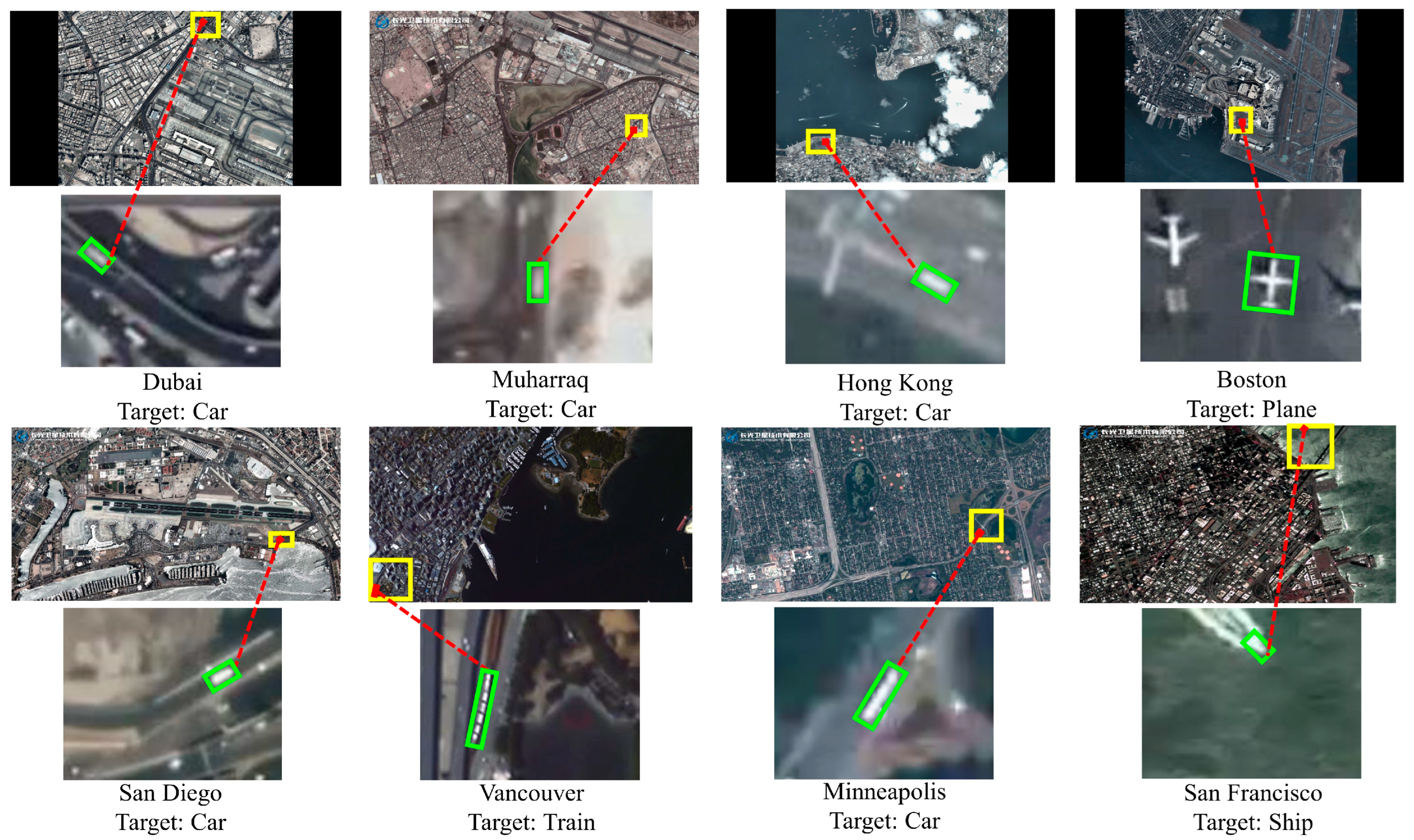
| SVs | Frame Size (px) | Cropped Region Size (px) | GSD (m) | Frame Number | Target | Target Size (px) | Rotation |
|---|---|---|---|---|---|---|---|
| Dubai | 4096 × 3072 | 256 × 218 | 0.92 | 147 | Car | 15 × 7 | √ |
| Muharraq | 4096 × 2160 | 174 × 193 | 0.92 | 500 | Car | 13 × 6 | √ |
| Hong Kong | 4096 × 3720 | 268 × 216 | 0.92 | 164 | Car | 14 × 7 | √ |
| Boston | 4096 × 3720 | 215 × 300 | 0.92 | 320 | Plane | 36 × 33 | √ |
| San Diego | 4090 × 2160 | 135 × 94 | 0.92 | 228 | Car | 13 × 6 | ─ |
| Vancouver | 3840 × 2160 | 501 × 487 | 0.92 | 405 | Train | 16 × 80 | ─ |
| Minneapolis | 4090 × 2160 | 336 × 328 | 0.92 | 268 | Car | 24 × 7 | ─ |
| San Francisco | 3840 × 2160 | 501 × 501 | 1.00 | 500 | Ship | 15 × 9 | ─ |
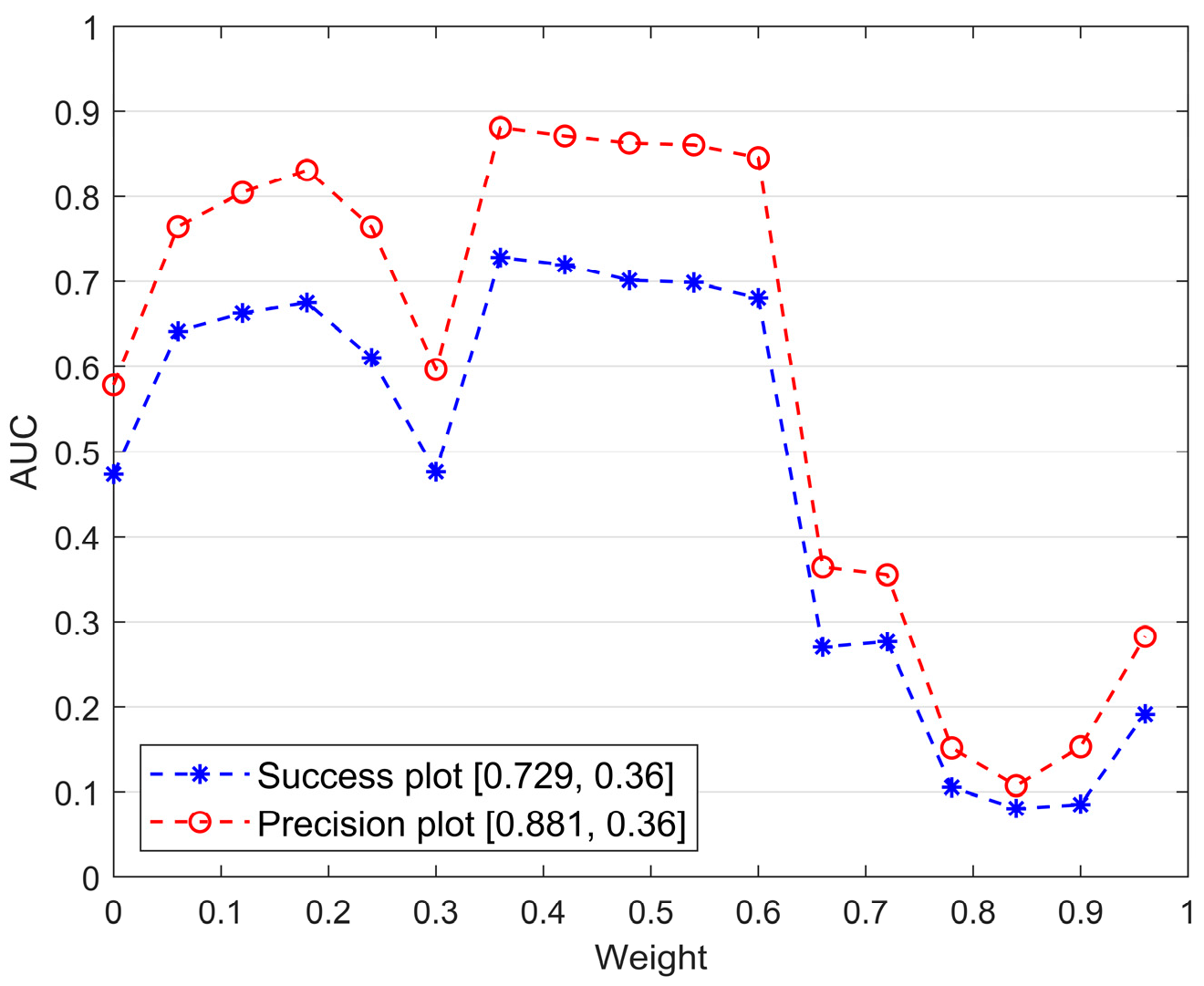
| Weights | 0 | 0.06 | 0.12 | 0.18 | 0.24 | 0.30 | 0.36 | 0.42 | 0.48 | 0.54 | 0.60 | 0.66 | 0.72 | 0.78 | 0.84 | 0.90 | 0.96 |
|---|---|---|---|---|---|---|---|---|---|---|---|---|---|---|---|---|---|
| Success plot | 0.473 | 0.642 | 0.663 | 0.675 | 0.611 | 0.476 | 0.729 | 0.720 | 0.701 | 0.699 | 0.681 | 0.270 | 0.277 | 0.106 | 0.081 | 0.085 | 0.192 |
| Precision plot | 0.579 | 0.765 | 0.805 | 0.831 | 0.764 | 0.597 | 0.881 | 0.871 | 0.863 | 0.861 | 0.846 | 0.364 | 0.355 | 0.152 | 0.108 | 0.153 | 0.283 |
| Trackers | KCF | +AE | +OFR | Success Plot | Precision Plot |
|---|---|---|---|---|---|
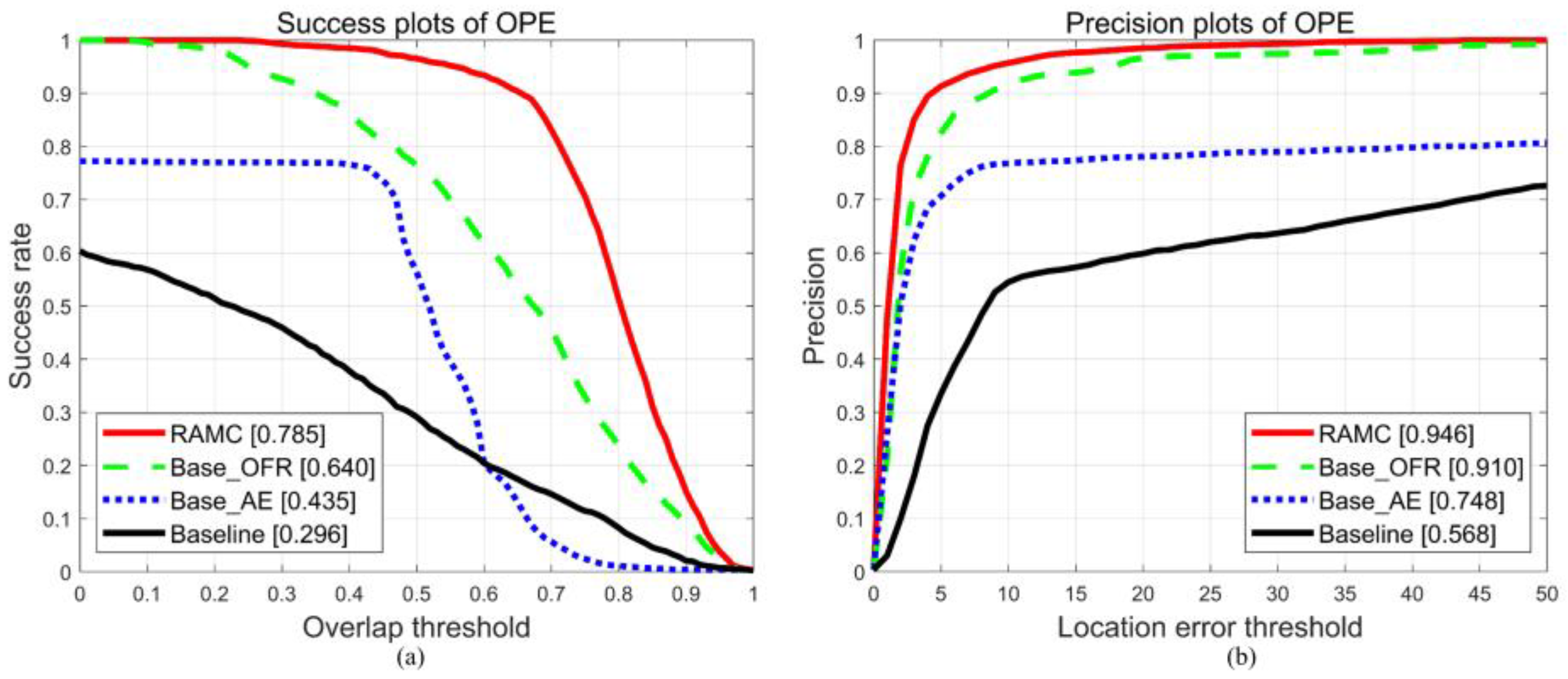
| Baseline | √ | ─ | ─ | 0.296 | 0.568 |
| Base_AE | √ | √ | ─ | 0.435 | 0.748 |
| Base_OFR | √ | ─ | √ | 0.640 | 0.910 |
| RAMC | √ | √ | √ | 0.785 | 0.946 |
| Trackers | Framework | Features | MR | MTD | Success Plot | Precision Plot | FPS |
|---|---|---|---|---|---|---|---|
| KCF (TPAMI 2015) | KCF | HOG | ─ | ─ | 0.296 | 0.568 | 231.53 |
| SAMF (ECCV 2014) | KCF | HOG + CN | ─ | ─ | 0.373 | 0.702 | 48.03 |
| BACF (ICCV 2017) | KCF | HOG | ─ | ─ | 0.508 | 0.884 | 52.98 |
| STRCF (CVPR 2018) | DCF | ConvFeat + HOG + CN | √ | ─ | 0.550 | 0.851 | 18.89 |
| AutoTrack (CVPR 2020) | DCF | HOG + CN | ─ | ─ | 0.606 | 0.916 | 51.90 |
| CFME (TGRS 2020) | KCF | HOG | ─ | √ | 0.613 | 0.855 | 104.36 |
| ASRCF (CVPR 2019) | KCF | ConvFeat + HOG | √ | ─ | 0.621 | 0.935 | 21.17 |
| SiamRPN (CVPR 2018) | SiameseFC | ConvFeat | √ | ─ | 0.625 | 0.910 | 62.76 |
| Staple (CVPR 2016) | DCF + II | HOG + CH | √ | ─ | 0.625 | 0.856 | 85.32 |
| GFS-DCF (ICCV 2019) | DCF | ConvFeat + HOG + CN | √ | ─ | 0.630 | 0.940 | 3.20 |
| LDES (AAAI 2019) | DCF | HOG + CH | √ | ─ | 0.647 | 0.824 | 21.72 |
| ECO (CVPR 2017) | CCF | ConvFeat | √ | ─ | 0.651 | 0.944 | 2.63 |
| SiamRPN++ (CVPR 2019) | SiameseFC | ConvFeat | √ | ─ | 0.723 | 0.951 | 33.03 |
| RAMC (proposed) | KCF | HOG + OF | √ | √ | 0.785 | 0.946 | 42.47 |
| Trackers | Rotation | Nrotation | ||
|---|---|---|---|---|
| Success Plot | Precision Plot | Success Plot | Precision Plot | |
| KCF (TPAMI 2015) | 0.399 | 0.707 | 0.194 | 0.429 |
| SAMF (ECCV 2014) | 0.464 | 0.815 | 0.283 | 0.589 |
| BACF (ICCV 2017) | 0.494 | 0.935 | 0.523 | 0.833 |
| STRCF (CVPR 2018) | 0.587 | 0.942 | 0.513 | 0.760 |
| AutoTrack (CVPR 2020) | 0.636 | 0.947 | 0.576 | 0.885 |
| CFME (TGRS 2020) | 0.513 | 0.769 | 0.714 | 0.940 |
| ASRCF (CVPR 2019) | 0.621 | 0.948 | 0.621 | 0.921 |
| SiamRPN (CVPR 2018) | 0.716 | 0.970 | 0.534 | 0.851 |
| Staple (CVPR 2016) | 0.681 | 0.956 | 0.568 | 0.757 |
| GFS-DCF (ICCV 2019) | 0.656 | 0.965 | 0.604 | 0.916 |
| LDES (AAAI 2019) | 0.569 | 0.715 | 0.724 | 0.933 |
| ECO (CVPR 2017) | 0.607 | 0.938 | 0.696 | 0.949 |
| SiamRPN++ (CVPR 2019) | 0.732 | 0.966 | 0.715 | 0.936 |
| RAMC (proposed) | 0.796 | 0.964 | 0.774 | 0.928 |
Publisher’s Note: MDPI stays neutral with regard to jurisdictional claims in published maps and institutional affiliations. |
© 2022 by the authors. Licensee MDPI, Basel, Switzerland. This article is an open access article distributed under the terms and conditions of the Creative Commons Attribution (CC BY) license (https://creativecommons.org/licenses/by/4.0/).
Share and Cite
Chen, Y.; Tang, Y.; Han, T.; Zhang, Y.; Zou, B.; Feng, H. RAMC: A Rotation Adaptive Tracker with Motion Constraint for Satellite Video Single-Object Tracking. Remote Sens. 2022, 14, 3108. https://doi.org/10.3390/rs14133108
Chen Y, Tang Y, Han T, Zhang Y, Zou B, Feng H. RAMC: A Rotation Adaptive Tracker with Motion Constraint for Satellite Video Single-Object Tracking. Remote Sensing. 2022; 14(13):3108. https://doi.org/10.3390/rs14133108
Chicago/Turabian StyleChen, Yuzeng, Yuqi Tang, Te Han, Yuwei Zhang, Bin Zou, and Huihui Feng. 2022. "RAMC: A Rotation Adaptive Tracker with Motion Constraint for Satellite Video Single-Object Tracking" Remote Sensing 14, no. 13: 3108. https://doi.org/10.3390/rs14133108
APA StyleChen, Y., Tang, Y., Han, T., Zhang, Y., Zou, B., & Feng, H. (2022). RAMC: A Rotation Adaptive Tracker with Motion Constraint for Satellite Video Single-Object Tracking. Remote Sensing, 14(13), 3108. https://doi.org/10.3390/rs14133108