Abstract
Groundwater-based irrigation has dramatically expanded over the past decades. It has important implications for terrestrial water, energy fluxes, and food production, as well as local to regional climates. However, irrigation water use is hard to monitor at large scales due to various constraints, including the high cost of metering equipment installation and maintenance, privacy issues, and the presence of illegal or unregistered wells. This study estimates irrigation water amounts using machine learning to integrate in situ pumping records, remote sensing products, and climate data in the Kansas High Plains. We use a random forest regression to estimate the annual irrigation water amount at a reprojected spatial resolution of 6 km based on various data, including remotely sensed vegetation indices and evapotranspiration (ET), land cover, near-surface meteorological forcing, and a satellite-derived irrigation map. In addition, we assess the value of ECOSTRESS ET products for irrigation water use estimation and compare with the baseline results by using MODIS ET. The random forest regression model can capture the temporal and spatial variability of irrigation amounts with a satisfactory accuracy ( = 0.82). It performs reasonably well when it is calibrated on the western portion of the study area and tested on the eastern portion that receives more rain than the western one, suggesting its potential transferability to other regions. ECSOTRESS ET and MODIS ET yield a similar irrigation estimation accuracy.
1. Introduction
Groundwater-based irrigation accounts for more than 70% of global freshwater use [1], especially in the arid and semi-arid regions [2,3]. The High Plains is one such region where groundwater-based irrigation has dramatically increased over the last decades and led to groundwater and streamflow depletions [4,5,6]. It is estimated that the cumulative groundwater depletion in the High Plains Aquifer (HPA) in the last century is over 353 km3, which is equivalent to a 1 mm sea-level rise [7]. Groundwater irrigation introduces additional water to the land surface and reduces the surface air temperature (the cooling effect) by shifting sensible heat to latent heat [8,9,10]. The latent heat, or evapotranspiration (ET), is further enhanced by the augmented available energy as a result of increased land greenness and decreased albedo of irrigated vegetation [10,11,12,13]. The extra atmospheric water vapor from the groundwater stimulates cloud cover and precipitation [9]. Nearly 80% of the extracted groundwater ends up in the ocean by surface runoff and increased precipitation caused by atmospheric vapor transport from the land to the ocean [14], which ultimately results in sea-level rise. On the other hand, groundwater depletion can also modify the monsoon circulation by changing the thermal contrast between the land and the ocean [15].
Despite the important implications of agricultural irrigation, discrepancies exist between the observations and numerical models in quantifying this human intervention in water cycles [16]. For example, Liu et al. [17] suggest a high bias (i.e., overestimation) in the temperature in the central US simulated by the Weather Research and Forecasting coupled to the Noah-Multiparameterization model (WRF/Noah-MP), especially during summer, likely due to the lack of representation of irrigation activity in the model. Scanlon et al. [18] indicate that the modeled terrestrial water storage (TWS) of seven global hydrologic models shows an opposite trend to that derived from the Gravity Recovery and Climate Experiment (GRACE), mainly due to the inability of the models to capture the human-induced water storage change. Adding an irrigation scheme to Noah-MP reduces the gap between the model simulation and the remotely sensed ET, GRACE TWS, and groundwater level measurements for the southern HPA, highlighting the importance of the enhanced representation of human water use [19].
The growing repository of in situ and remote sensing observations and data fusion techniques provide opportunities to develop a retrospective dataset of groundwater irrigations [20]. Two commonly used types of remote sensing data for irrigation estimation are soil moisture (SM) and ET. SM products from Soil Moisture Active Passive (SMAP), Soil Moisture and Ocean Salinity (SMOS), Advanced SCATterometer (ASCAT), and Advanced Microwave Scanning Radiometer (AMSR2) have been used to detect irrigation areas [21,22,23,24,25]. Methods have also been developed to quantify irrigation amounts using SM data. For example, Brocca et al. [26] calculate irrigation as the difference between storage change (from remotely sensed SM) plus outflow (drainage and ET calculated using an SM balance model) and in situ rainfall measurements at pilot sites located in the U.S., Europe, Africa, and Australia. Other studies extend this method with various estimated and remote sensing ET products [27,28,29]. Zaussinger et al. [30] infer the monthly irrigation water use over the contiguous United States (CONUS) based on the gap between remote sensing SM and Modern-Era Retrospective Analysis for Research and Applications Version 2 (MERRA-2) reanalysis SM that does not include irrigation. Zappa et al. [31] further incorporate calculated ET and drainage loss for their study sites in Germany into this method. Studies have also estimated the irrigation amount by comparing precipitation to remotely sensed ET, such as the MODIS (Moderate Resolution Imaging Spectroradiometer) product (MOD16A). More specifically, MODIS ET, which is treated as the ground truth crop ET rate, surplus over the effective precipitation or Land Surface Model (LSM) simulated ET, is treated as a crop consumptive water use supplied by irrigation [27,32,33,34,35,36].
The above approaches based on water balance rely heavily on the accuracy of the remote sensing and reanalysis products. Due to the coarse resolution and uncertainty of remote sensing SM [26,27], these approaches often perform less well for low-intensity irrigation signals, such as supplementary irrigation, irrigation in semi-humid and humid areas, and irrigation with high-efficiency technology [26,27,30]. In parallel, various irrigation schemes have been developed within LSMs to derive irrigation driven by crop demands [19,37]. However, these LSMs’ capability of predicting SM is questionable considering the uncertainties in the upper (e.g., infiltration of ponding water and runoff) and lower boundary conditions (e.g., groundwater exchange).
Irrigation water management is heavily dependent on socioeconomic-controlled irrigation behavior, including local policy, water rights, and farm producer irrigation preferences [37,38,39,40]. Irrigation schemes implemented in LSMs often fall short of representing the socioeconomic controls on irrigation behavior. Machine learning algorithms and remote sensing data provide opportunities to capture human–water interactions that are hard to represent using physically based methods [39,41,42,43,44,45]. Several studies have applied machine learning approaches in the High Plains region to map irrigated farmlands [46], identify irrigation driving factors [38], and estimate groundwater withdrawal from MODIS ET [47].
We present a machine learning approach for estimating spatial irrigation amounts by fusing hydrometeorological, in situ, and multi-source remote sensing data that reflect dynamic crop conditions. Our approach is applied over the Kansas HPA, where in situ pumping records [48] are available for training and validating the machine learning model. Through a spatial prediction experiment, we demonstrate the potential transferability of our approach to other regions with scarce or no in situ pumping records to create an annual, gridded irrigation amount dataset, which can then be used to improve the representation of anthropogenic irrigation within ecohydrological and atmospheric models and enhance the prediction capability of regional land–atmosphere feedbacks. In addition, we compare the irrigation estimation accuracy using the recently available ECOsystem Spaceborne Thermal Radiometer Experiment on Space Station (ECOSTRESS) ET products and MODIS ET.
2. Datasets and Methodology
2.1. Study Area
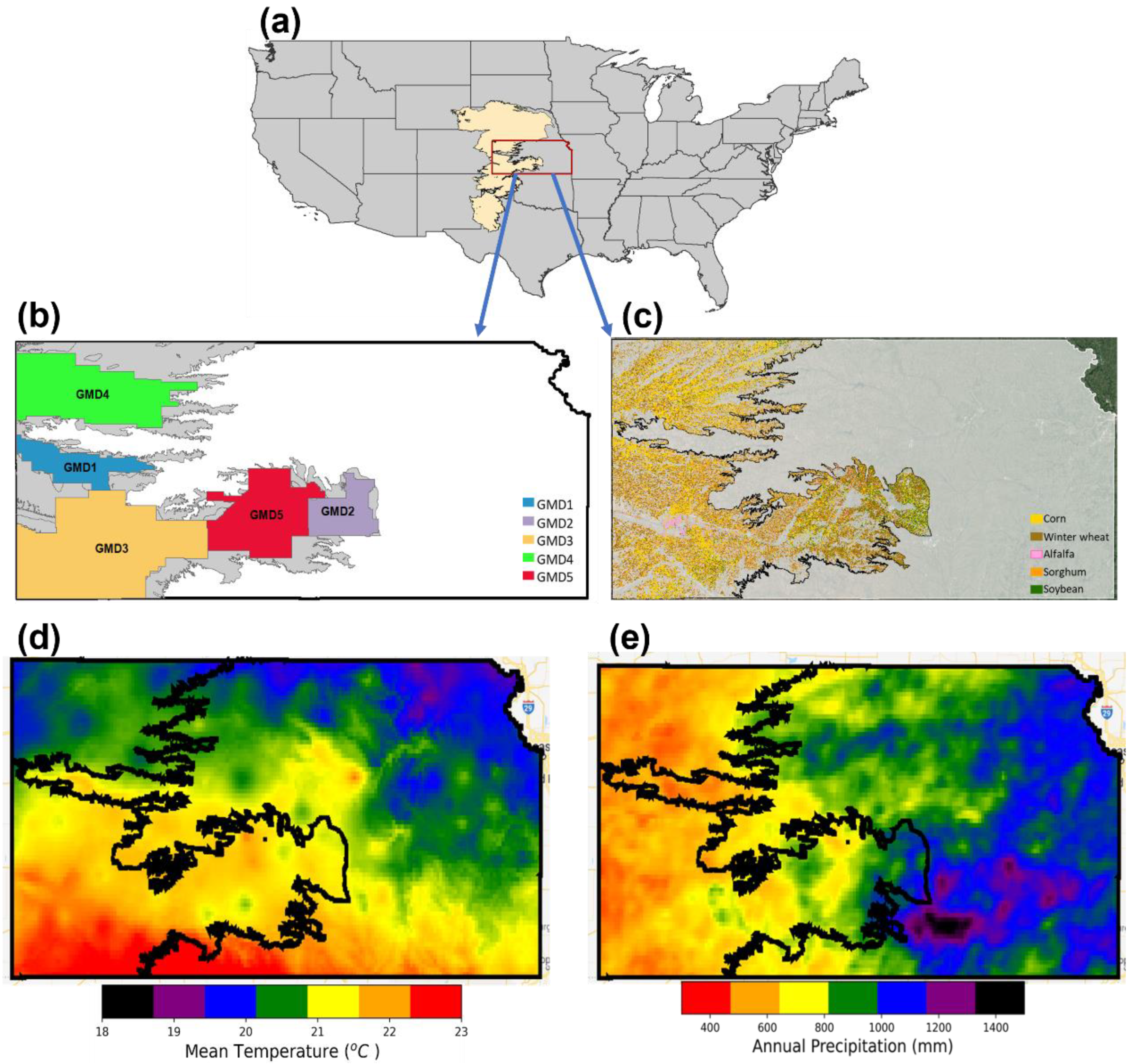
Our study area is a portion of the central HPA in Kansas (Kansas HPA, Figure 1a). In recognition of the “lead from local need” perspective, five groundwater management districts (GMDs) were established in the 1970s (Figure 1b) for water use administration and planning [49]. The primary crop types in this region are winter wheat, corn, soybeans, sorghum, and alfalfa [50] (Figure 1c). The study area experiences a climatic gradient from semi-arid in the west to sub-humid in the east and a decreasing temperature from south to north (Figure 1d,e; [51]). The agriculture of Kansas HPA heavily relies on irrigation to meet crop water demands. The Kansas Geological Survey Water Information Management and Analysis System (WIMAS) [48] dataset provides a continuous annual irrigation water use record reported by individual water right holders since 1990. For over 95% of the irrigation wells in Kansas HPA, the reported water use volume is measured by totalizing flowmeters [51]. The non-metered wells are required to provide pumping hours and pumping rates to ensure the reported data quality [52].

Figure 1.
(a) Extent of the High Plains Aquifer (HPA), (b) Kansas portion of HPA and five groundwater management districts (GMDs), (c) distribution of major crop types, (d) mean annual temperature (°C) and (e) annual precipitation (mm) in 2016, a year with normal hydrometeorological conditions.
2.2. Data Collection
We compiled various remote sensing products, climate data, and ancillary information (Table 1, Figure 2) to estimate irrigation using a machine learning model. All data were aggregated into a 6 km × 6 km spatial resolution, which can be readily adapted to the model’s needs. We further aggregated time-varying remote sensing and climatic data to an annual scale. For these data sources, we chose to focus on 1 May–31 August (MJJA), which covered most of the growing season, according to the planting and harvesting schedule of primary crop types in the study area [53,54]. The remote sensing data include the Normalized Difference Vegetation Index (NDVI), Normalized Difference Water Index (NDWI), and Greenness Index (GI), and ET products. The vegetation indices (NDVI, NDWI, GI) were calculated from 30 m-resolution Landsat 5, Landsat 7, and Landsat 8 surface reflectance images, respectively. Due to the differences in band designations and sensors [55,56], we normalized the vegetation indices from each Landsat image by linearly scaling them to the range of [0, 1] before aggregating to the annual scale. We used the following three ET products: MODIS 8-day 500 m resolution ET (MOD16) [57], ECOSTRESS PT-JPL instantaneous ET [58], and ECOSTRESS DisALEXI-JPL daily ET [59]. Both DisALEXI-JPL and PT-JPL products are at a 70 m resolution using the ECOSTRESS Level 1 geolocation information, Level 2 Land Surface Temperature (LST) and Emissivity product, near surface temperature, wind speed and relative humidity from National Centers for Environmental Prediction (NCEP), and data from MODIS and LANDSAT 8. The ECOSTRESS DisALEXI-JPL daily ET is based on an Atmosphere–Land Exchange Inverse (ALEXI) surface–energy balance model. The ECOSTRESS PT-JPL is based on the Priestley–Taylor (PT) method [60] and available both as instantaneous (i.e., at the overpass time) and daily rates. We used the instantaneous product because the daily product is interpolated from the instantaneous ET assuming a clear sky diurnal solar cycle. As a result, the daily ECOSTRESS PT-JPL ET product tends to overestimate, especially in frequently cloud-covered regions [61].
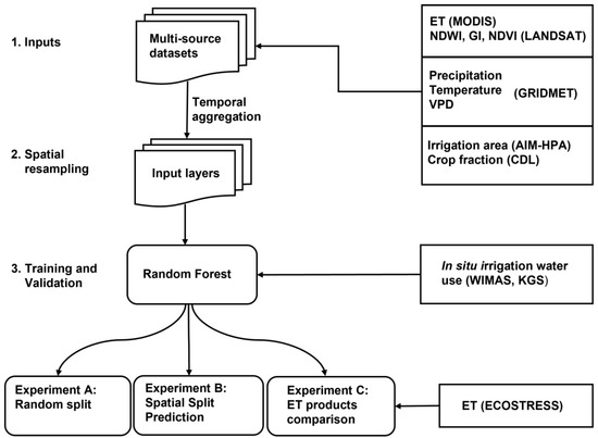
Figure 2.
Flowchart of a machine learning-based estimation of the spatial irrigation amount by fusing hydrometeorological data, in situ irrigation water use records, multi-source remote sensing data, and derived irrigation maps and crop fractions.
The second group of inputs was calculated from GRIDMET climate data [62], including daily maximum temperature, total precipitation, and daily mean water vapor deficit (VPD). The third group of inputs were derived products of land use and land cover, including annual irrigation maps for HPA (AIM-HPA) [46] and crop fractions. The AIM-HPA dataset identifies irrigated fields at a 30 m resolution and was derived based on Landsat imagery, hydroclimatic data, and ancillary information, such as the USDA Soil Survey Geographic Database (SSURGO). The irrigation maps were resampled to the 6 km resolution used in this study by calculating the percentage of the irrigated area within one 6 km × 6 km grid. Lastly, we calculated crop fractions based on the USDA National Agricultural Statistics Service Cropland Data Layers [63] (available since 2006) as the percentage of the cultivated area of each primary crop type in a 6 km × 6 km grid.

Table 1.
Datasets used to generate input and target variables.
Table 1.
Datasets used to generate input and target variables.
| Variables | Product | Temporal Aggregation | Reference |
|---|---|---|---|
| ET | MOD16A | Sum of MJJA | [64] |
| ET | ECOSTRESS PT-JPL | Sum of MJJA | [65] |
| ET | ECOSTRESS dis-ALEXI | Sum of MJJA | [66] |
| NDVI, NDWI, GI | LANDSAT | Mean of MJJA | [67] |
| Precipitation | GRIDMET | Sum of MJJA | [62] |
| Daily maximum temperature | GRIDMET | Mean of MJJA | [62] |
| Water vapor deficit (VPD) | GRIDMET | Mean of MJJA | [62] |
| Irrigated area | AIM-HPA | Annual | [46] |
| Crop fraction | CDL | Annual | [63] |
| In situ irrigation water use | WIMAS | Annual | [48] |
2.3. Methods
We used random forest regression (RFR) to estimate the irrigation amount from the input datasets (Table 1). The irrigation amount was represented as depth by dividing the total volume of the irrigation water use within each 6 km × 6 km grid by the area of the grid (36 km2). A random forest is an ensemble of decision trees with bootstrap sampling [68]. By averaging the results across all trees and randomly choosing a subset of variables at each split point, the RFR is less prone to overfitting than a single tree [68]. RFR has been used in many remote sensing applications as it can manage high dimensional, correlated data with easy hyperparameter tuning and a relatively fast process [69]. In this study, we trained and validated RFR models using the in situ irrigation records as targets. We also used variable importance scores to examine the contribution of each variable to the estimation accuracy. The variable importance was calculated based on the Gini impurity, measuring how splitting with an input variable decreases the impurity (variance) of the data [70]. The performance of the model was evaluated by root-mean-square error (RMSE), coefficient of determination (), and percentage bias (PBIAS) statistics calculated using in situ irrigation records reserved for the validation. The PBIAS measures the average trend of the predicted value to be larger or smaller than the actual value [71].
We performed three experiments to test the prediction skill of the RFR model, probe its potential for transferability, and investigate the utility of the ECOSTRESS ET for an annual irrigation amount estimation (Figure 2). In Experiment A, we randomly split the data across the study area from 2006 to 2020 into 70% for training and 30% for test. To examine the capability of the RFR model to capture the overall spatial and temporal variability of the irrigation amount, we trained the RFR model with all years’ training data and assessed the accuracy of the trained model on the validation data points each year.
In Experiment B, we split the data from 2006 to 2017 by region. More specifically, we divided the model domain into the western and eastern portions for training and test, respectively. Given the differences in climate conditions and crop types between the training and test regions (Figure 1c–e), this experiment represents a challenging case and was designed to investigate the spatial transferability of our approach. Since the ECOSTRESS ET product was not available until late 2018, Experiments A and B were performed using MODIS ET.
In Experiment C, we performed the same random split test for years 2019 and 2020 using the ECOSTRESS in one run and the MODIS ET in another run. We compared the accuracy resulting from the use of the ECOSTRESS and MODIS ET products.
3. Results
3.1. Experiment A: Random Split
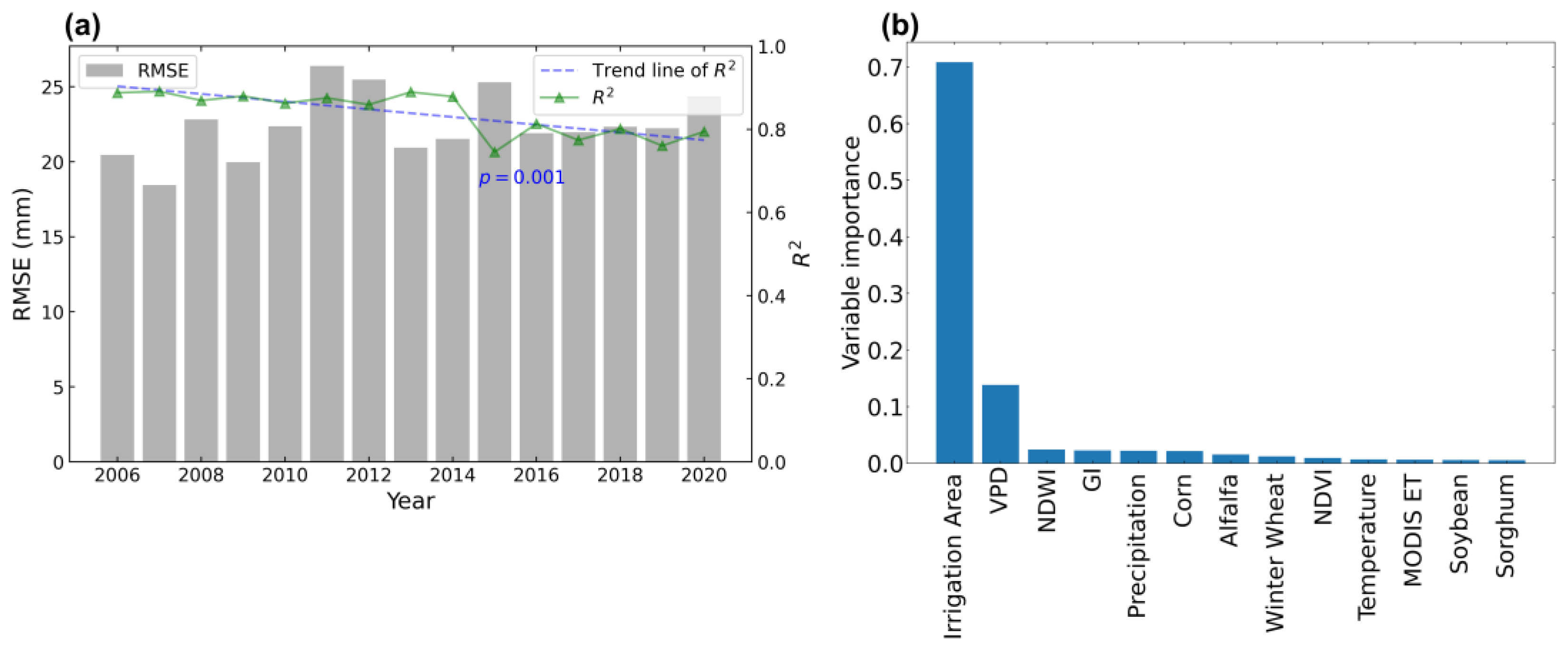
Overall, the RFR achieves satisfactory performance, with an average RMSE, PBIAS, and of 22.9 mm, −0.73%, and 0.82, respectively (Figure 3). Despite interannual variabilities, a declining trend in is noticeable primarily due to the decreasing variability of the irrigation amount among the grids in the study area (Figure S2). The decrease in variability suggests that the irrigation behavior became more homogeneous. Possible causes may be water use being constrained by local water conservation programs and the expansion of water-saving irrigation technology during the study period, which will be further discussed in Section 4. Figure 3b shows the variable importance scores calculated by the RFR for the inputs listed in Table 1. The irrigation area from the AIM-HPA dataset [46] receives the highest score. This is not surprising, since a higher irrigation area is directly related to higher irrigation amounts. It is noteworthy that the AIM-HPA dataset is available for the entire HPA and does not rely on irrigated acreage records. This enables our approach to be extended to other parts of HPA, where in situ records such as WIMAS are not available. The irrigation area is correlated with remote sensing vegetation indices, thus, overshadows the vegetation indices in terms of variable importance scores (Figure 3b).
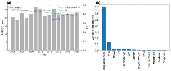
Figure 3.
Results from Experiment A (random split), including (a) annual root-mean-square error (RMSE) and coefficient of determination () from 2006 to 2020; Linear regression of shows a statistically significant declining trend (); (b) Random forest variable importance scores.
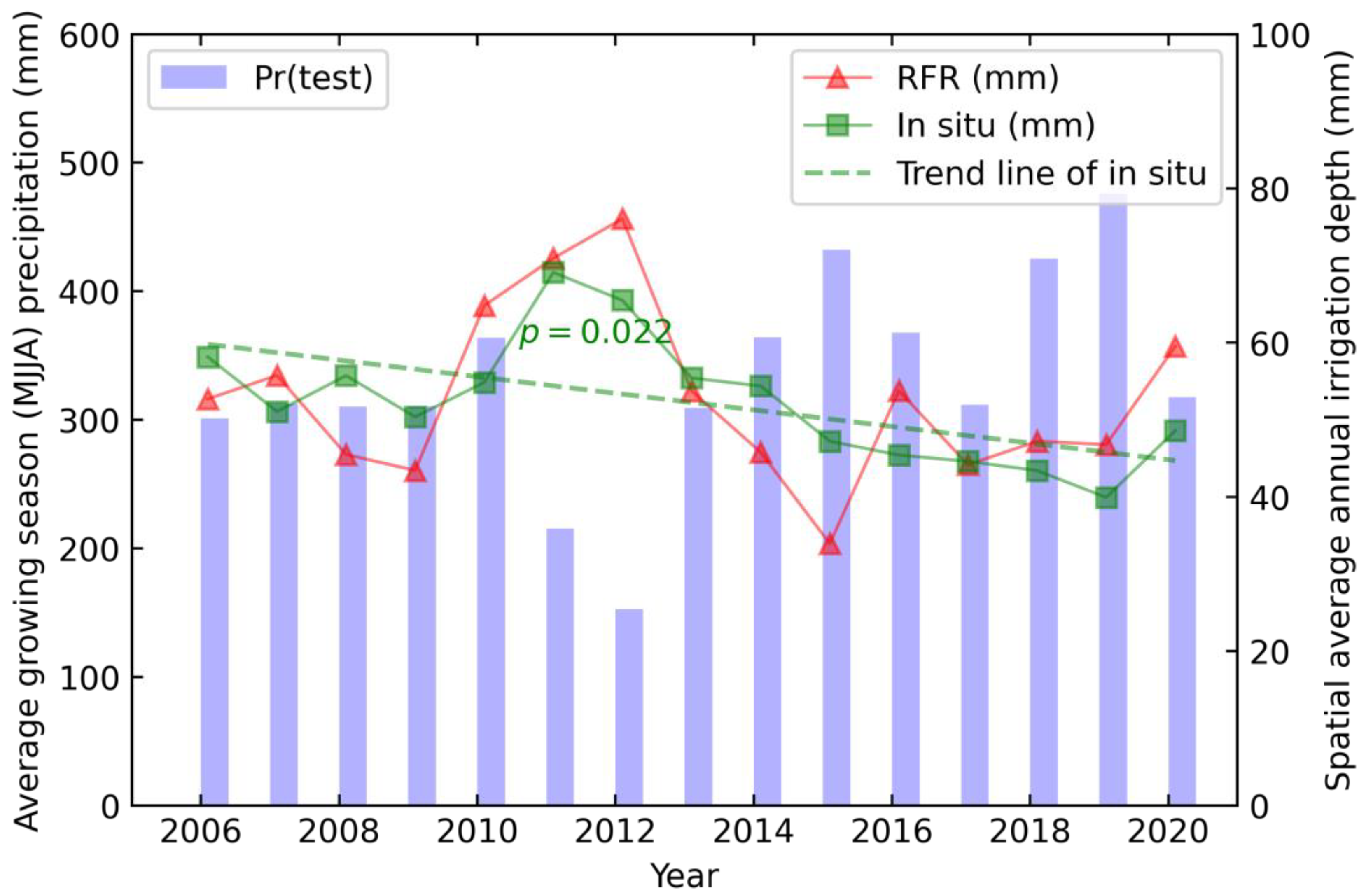
The irrigation volume of the Kansas HPA predicted by the RFR overall follows the interannual variability in the in situ irrigation records from WIMAS (Figure 4). Both the in situ and estimated irrigations peaked in 2011 and 2012, which were drought years with lower-than-usual growing season precipitation (Figure 4). The RFR model tends to perform better in dry years than in wet years (e.g., 2015, 2019) (Figure S1). The RFR continuously overpredicts the annual irrigation amount over Kansan HPA since 2016. This may be due to irrigation technology and water management policy changes, as discussed in Section 4.1.
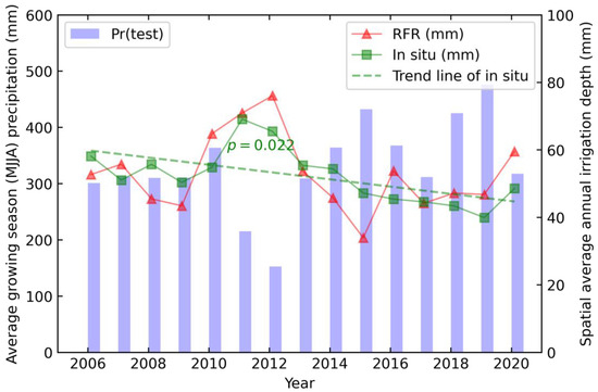
Figure 4.
Annual growing season (May, June, July, August, MJJA) total precipitation (bars) and irrigation amounts as depth (mm) from the RFR (red, triangle) and in situ records (green, square) for the entire Kansas HPA from 2006 to 2020 in Experiment A (random split). Linear regression (green, dashed) of the in situ irrigation amount has a decreasing trend (. The irrigation amount estimated by the RFR does not have a statistically significant decreasing trend.
3.2. Experiment B: Spatial Split
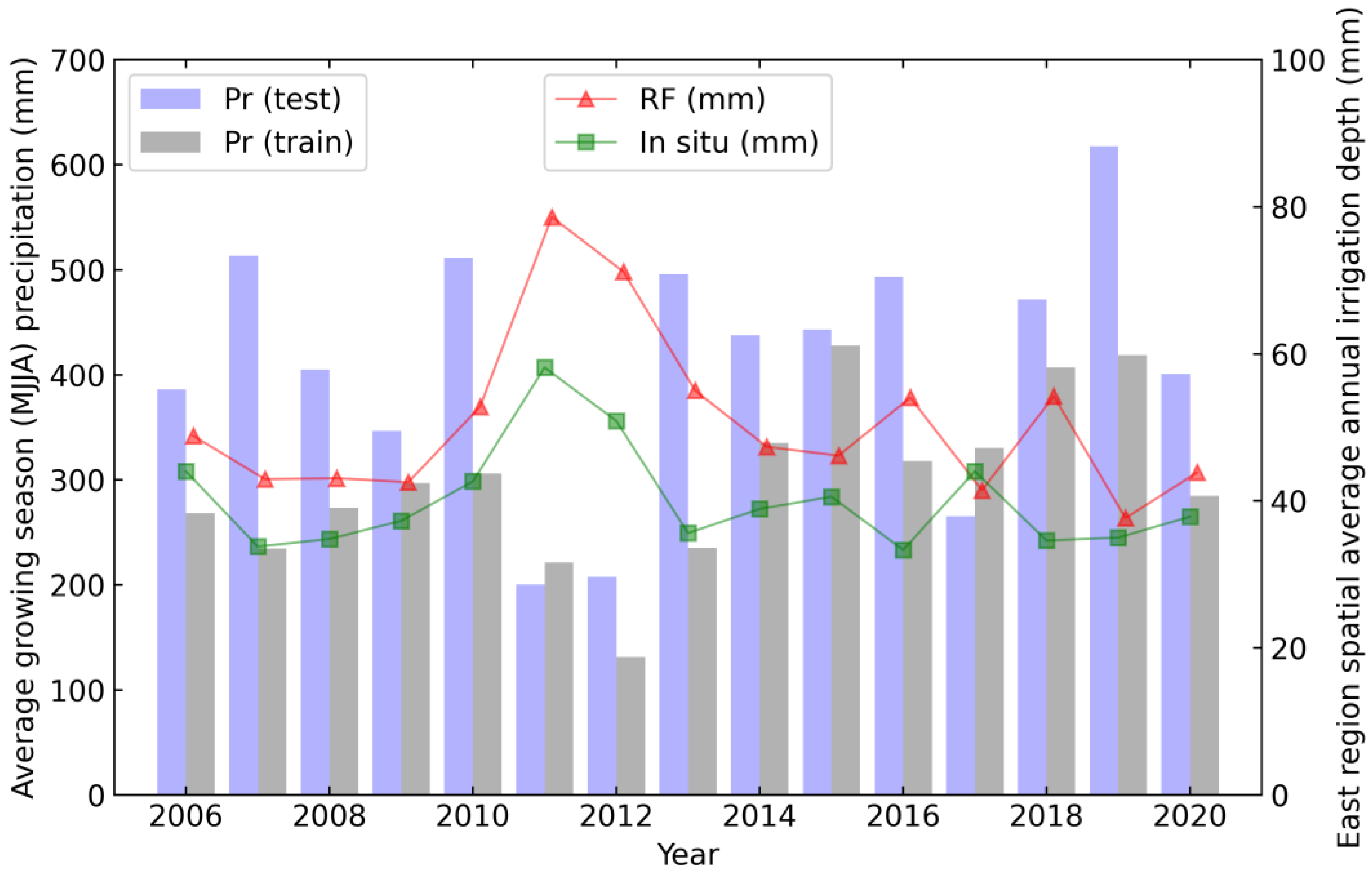
The RFR model achieved a lower but still satisfactory accuracy in the Experiment B spatial split test (Figure 5 and Figure 6) than in Experiment A (random split). Noteworthy, the annual precipitation during the study period was in the range of 431–635 mm for the training region and 584–863 mm for the test region. The RFR predicted irrigation amount for the test region is systematically higher than in situ records, suggesting an overestimation. Nevertheless, the RFR prediction is overall following the interannual variability of the in situ records. For example, the peak irrigation amount from the RFR estimation and the in situ records both occurred in 2011 and 2012. This is the same as in Experiment A and consistent with the drought conditions in the two years.
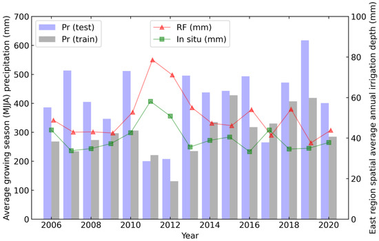
Figure 5.
Annual irrigation amounts from the RFR (red triangles) and in situ records (green squares) for the test data (eastern portion of Kansas HPA) in Experiment B (spatial split). The growing season (May, June, July, August, MJJA) total precipitations for training (grey bars) and test (purple bars) portions, respectively, are also shown.

Figure 6.
Spatial distribution of (a) in situ and (b) RFR estimated irrigation amounts in Experiment B (spatial split) for a medium model performance year (2011). The red dashed line divides the training (western) and test (eastern) portions.
We also examined the spatial distribution of the irrigation amounts of the in situ records and RFR estimates, respectively, for a moderate model performance year (Figure 6) and other years (Figures S3 and S4). The dashed line separates the training (western) and test (eastern) portions of the study area. When trained over the western Kansas HPA, the RFR model is able to capture the spatial variability of the irrigation amounts in the eastern Kansas HPA reasonably well despite a slight overestimation.
3.3. Experiment C: ECOSTRESS and MODIS ET Comparison
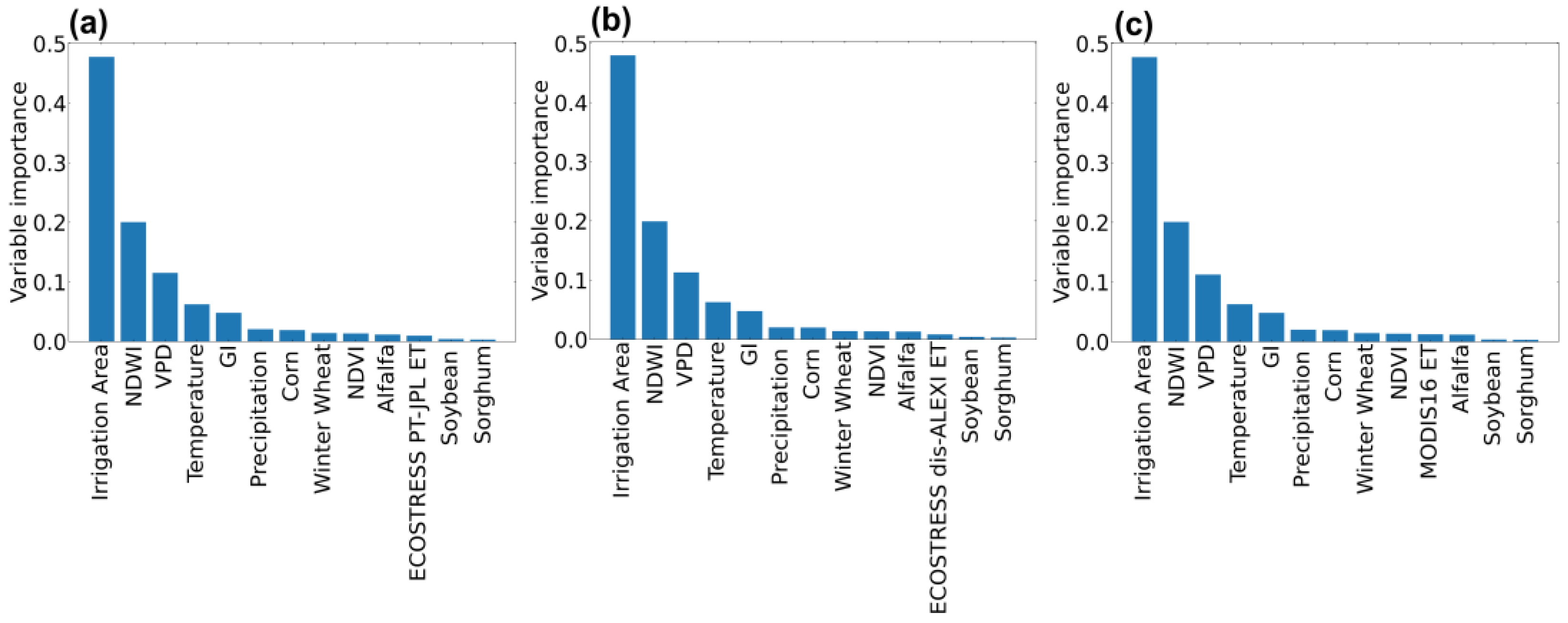
Table 2 lists the PBIAS, RMSE, and metrics resulting from Experiment C (see Section 2.2). To constrain the uncertainty from random sampling in the random forest algorithm, the RFR was repeated 200 times, and the mean and standard deviations of the metrics are reported. Based on the three metrics, ECOSTRESS PT-JPL, dis-ALEXI, and MOD16 ET products yield irrigation volume estimates of similar accuracy. The average variable importance scores calculated by repeating the RFR 200 times using each ET product show that MOD16 ET receives a slightly higher importance score than ECOSTRESS ET products (Figure 7). However, all ET products appear to be less important than the irrigation area, hydrometeorological data, and vegetation indices. It is also noteworthy that the vegetation indices receive a higher importance score in Experiment C than in Experiment A. This may be because these variables became more important for capturing spatial irrigation patterns during a shorter time period (2 years).

Table 2.
Mean value and standard deviation (STD) of percent bias (PBIAS), root-mean-square error (RMSE), and coefficient of determination () on test data for 2019–2020 from 200 repetitions of the RFR using three ET datasets.

Figure 7.
Input variable importance scores calculated by the RFR (averaged from 200 times of repeated tests) using (a) ECOSTRESS PT-JPL instantaneous ET, (b) ECOSTRESS dis-ALEXI ET, and (c) MOD16 ET.
4. Discussion
4.1. Groundwater Irrigation Trend
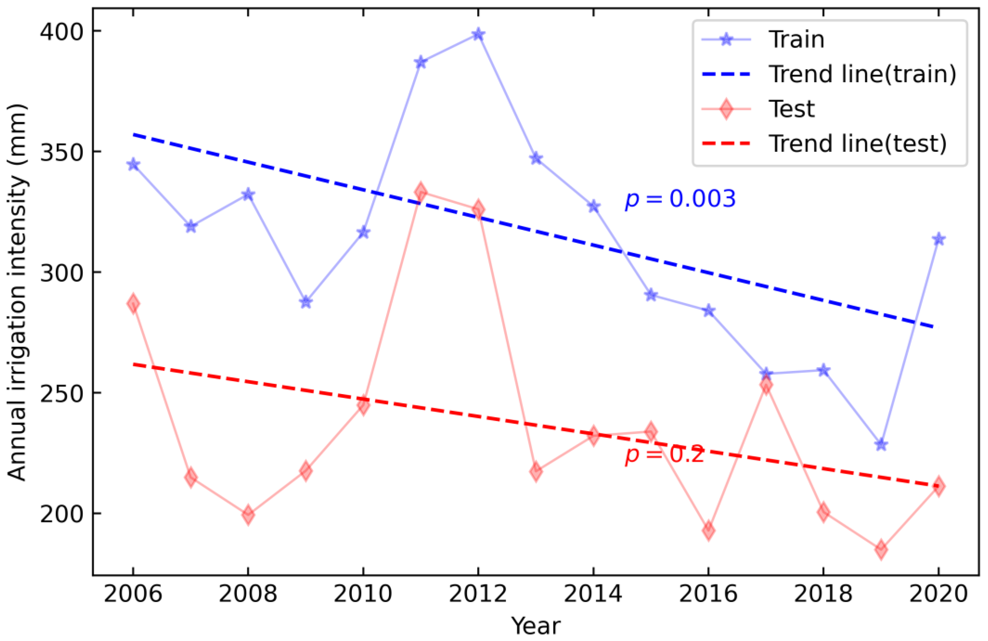
Despite the strong climatic control on the irrigation amount interannual variability (e.g., higher irrigation in drought years), irrigation water use has overall decreased in the Kansas HPA during the study period. The declining trend is primarily due to irrigation management policy and irrigation technology changes in recent years [40,72]. Since 2006, most Kansas HPA irrigation fields have adapted central pivot irrigation to central pivot with Low Energy Precise Application (LEPA). The LEPA technology can reduce wind drift-caused ET, therefore, improving the irrigation efficiency and reducing the irrigation intensity (or irrigation volume per irrigated area) required for crop growing [73]. Figure 8 shows the spatially averaged irrigation intensity during the study period for the training (western) and test (eastern) portions of the study area. It was calculated by dividing the total irrigation amount of each grid with the irrigated acreage in that grid (as opposed to the grid size, 36 km2, used to calculate the irrigation depth) and taking the average across the Kansas HPA. Both the irrigation amount and irrigated acreage are from the WIMAS dataset.
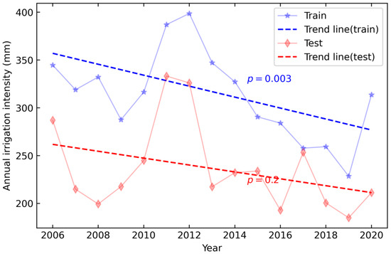
Figure 8.
Spatially averaged annual irrigation intensity calculated for the training and test portions of the Kansas HPA in Experiment B.
The declining trends in irrigation amount and intensity can also be attributed to the Local Enhanced Management Area (LEMA) groundwater conservation program. The LEMA was initially introduced in the GMD 4 Sheridan County 6 from 2012 and has been expanding within GMD 4 and to other GMDs since then [40,74,75]. Irrigators participating in the LEMA project either switched to water conservation crops or reduced the irrigation intensity, resulting in decreased irrigation amounts [73].
Despite the declining irrigation amount, the study period has experienced an increase in the irrigated area, according to the AIM-HPA dataset (Figure S5). Given the high importance score received by the irrigation area, the accuracy of the irrigation amount estimation is sensitive to the accuracy of the AIM-HPA. A higher irrigation area in later years likely contributed to the overestimation of the irrigation amounts after 2015. While AIM-HPA has been validated using the USDA National Agricultural Statistics Service (NASS) records at county level and achieved an = 0.86 to 0.93 for counties within the central High Plains region, the map tends to have commission (false positive) errors in humid climate areas with rainfed crops [46]. Therefore, it might overestimate the irrigation area within our study area.
Declining trends were found in the GI and NDVI during the study period (Figure S6). However, NDWI exhibited an increasing trend, seemingly contradictory to the expectation that a reduced irrigation intensity would result in a lower NDWI. Given the opposite trends and low importance scores received by these indices, they are likely overshadowed by the irrigation areas that have increased over years. Therefore, the declining trend in the irrigation amounts caused by irrigation policy and technology changes is not adequately captured by the input variables used in this study. In Experiments A and B, the RFR model was trained and tested using data throughout the study period. The trained RFR model sought an overall goodness-of-fit; thus, it learned the “average” irrigation behavior. Therefore, the RFR slightly underestimated the annual total irrigation amount in earlier years, while it overestimated it in later years of the study period (Figure 4). Including irrigation technology and policy information in the model inputs (e.g., LEMA regulated the cultivated area fraction of each grid) might improve the estimation accuracy, although limiting the transferability of our approach to other regions without such information.
4.2. Spatial Transferability
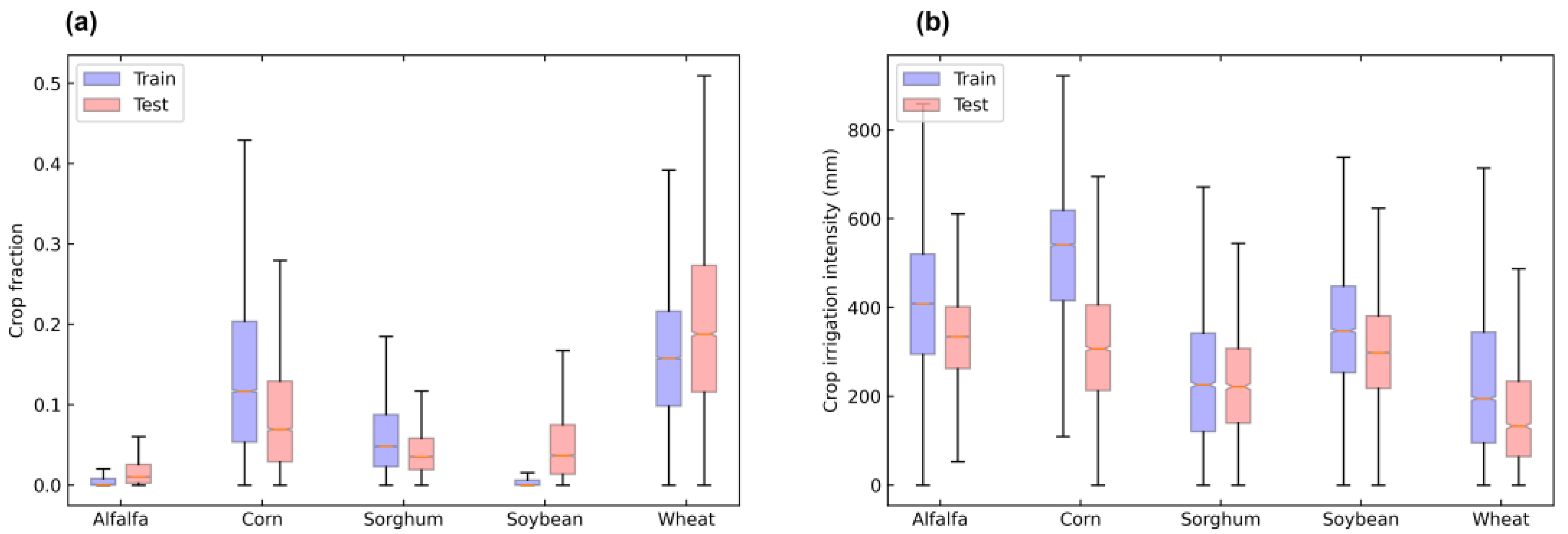
In addition to the temporal shift in irrigation technology and practices, the study area exhibits a spatial variability of climatic conditions, crop types, and irrigation practices that are typical for HPA. Experiment B is a challenging case where the training and test datasets differ in climate, crop types, and irrigation practices to examine the spatial transferability of our approach. The western part (GMDs 1, 3, and 4) is dryer; thus, it needs an overall higher irrigation amount than the eastern part (GMDs 2 and 5). Additionally, the training and test areas differ in fractions of the major crops. In particular, the test region has substantially more soybeans and alfalfa than the training region (Figure 9a). Overall, the major crops had a higher irrigation intensity in the dryer training region (Figure 9b). As a result, the training and test data in Experiment B have different input distributions. Predicting at a data point different from the training data (out-of-distribution) is a well-known challenge for machine learning techniques [76]. By using a variety of input variables, such as remote sensing-derived data, our approach partially overcomes the out-of-distribution challenge. The RFR is shown to be relatively skillful in capturing the inter-annual and spatial variability in irrigation amounts in Experiment B. This suggests that our approach of estimating irrigation amounts using remote sensing and hydroclimatic data can be potentially extended to other parts of the HPA.
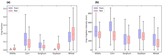
Figure 9.
Boxplots of (a) crop fractions (the area of each crop in a grid divided by the total grid area) and (b) irrigation intensity of major crop types in Experiment B training and test regions, respectively, in Kansas HPA, averaged during 2006–2020.
4.3. ECOSTRESS ET Utility for Irrigation Amount Estimation
Despite their higher spatial resolution and accuracy, the ECOSTRESS ET products (dis-ALEXI daily and PT-JPL instantaneous) generated irrigation estimations similarly accurate as the results from MODIS ET. This is likely due to the low variable importance scores received by the ET products. Since ET is highly correlated to VPD, its importance as an explanatory variable for irrigation amounts may have been overshadowed by VPD. Uncertainty associated with remote sensing ET products further reduces their information content for estimating irrigation amounts. Another reason for the similar accuracy of using ECOSTRESS and MODIS ET may be the low temporal and spatial coverage of the ECOSTRESS images. As a result, important irrigation information during the growing season may be missed. Recent work on fusing the ECOSTRESS ET with spatially coarser yet temporally continuous ET products, such as MODIS [77], to generate a high spatial and temporal resolution ET holds great potential to further improve irrigation amount estimations.
5. Conclusions
In this research, we develop a random forest regression model to fuse multiple remote sensing products, hydrometeorological information, and in situ annual irrigation records in the Kansas portion of the HPA to estimate annual irrigation amounts at a 6 km spatial resolution. Specifically, we use remote sensing ET products, vegetation indices (GI, NDVI, NDWI), crop types, climate data (precipitation, temperature, water vapor deficit), and a remote sensing-derived irrigation map dataset as input variables and train a random forest model using in situ irrigation records. In all three experiments, the RFR model achieves a satisfactory performance and generates annual irrigation estimates in good agreement with in situ records. The spatial split test with spatially different climates and irrigation patterns between the training and test regions, which appears to be the most challenging, indicates that the RFR can still capture the irrigation patterns relatively well, thus, suggesting the model’s potential for spatial transferability. Finally, the irrigation amounts estimated at the 6 km resolution using two ECOSTRESS ET products (dis-ALEXI daily and PT-JPL instantaneous) have a similar accuracy compared with the MODIS ET results. This is likely due to the low importance scores received by the ET products and their correlation with the VPD, as well as the ECOSTRESS images may miss key irrigation periods due to their low spatial and temporal coverage. However, the high spatial resolution of the ECOSTRESS ET is vital for estimating irrigation amounts at the field scale. In addition, recent advances in developing a fused ET product that has high spatial and temporal resolutions could further improve the accuracy of irrigation amount estimations.
Supplementary Materials
The following supporting information can be downloaded at: https://www.mdpi.com/article/10.3390/rs14133004/s1, Figure S1: Experiment A (random split) test varies with the growing season (MJJA) precipitation amounts for 2006–2020; A statistically significant ( = 0.02) linear declining trend is also shown; Figure S2: Annual variance of in situ irrigation depth (mm2) of the test data in Experiment A (random split). Also shown is a statistically significant declining trend ( = 0.03); Figure S3: (a) In situ and (b) RFR estimated irrigation amounts in Experiment B (spatial split) for the low performance year 2020 with an = 0.37. The red dash line divides the training (western) and test (eastern) regions; Figure S4: (a) In situ and (b) RFR estimated irrigation amounts in Experiment B (spatial split) for the good performance year 2006 with an = 0.77. The red dash line divides the training (western) and test (eastern) regions; Figure S5: Annual total irrigation acreage within the study area from in situ records (WIMAS, purple) and a remote sensing derived irrigation map (AIM-HPA, grey); Figure S6: Normalized annual GI (green, triangles), NDVI (red, squares), and annual NDWI (blue, circle) averaged across the study area during 2006–2020. Linear regression lines of GI, NDVI, and NDWI are also shown with -values.
Author Contributions
Conceptualization, R.Z. and T.X.; methodology, T.X., R.Z. and S.W.; software, S.W.; validation, S.W.; formal analysis, S.W.; data curation, S.W.; writing—original draft preparation, S.W., T.X. and R.Z.; writing—review and editing, all authors; visualization, S.W.; supervision, T.X. and R.Z.; project administration, R.Z.; funding acquisition, R.Z., T.X. and G.-Y.N. All authors have read and agreed to the published version of the manuscript.
Funding
This research was funded by NOAA COM Grant NA20OAR4310341.
Data Availability Statement
All data used in this research are publicly available. The data and code used for training and testing the machine learning model are available at https://github.com/shiqi572/EstimatingIrrigationKansasHPA.
Acknowledgments
The authors thank Jillian Deines for sharing the AIM-HPA dataset.
Conflicts of Interest
The authors declare no conflict of interest.
References
- Siebert, S.; Burke, J.; Faures, J.M.; Frenken, K.; Hoogeveen, J.; Döll, P.; Portmann, F.T. Groundwater Use for Irrigation—A Global Inventory. Hydrol. Earth Syst. Sci. 2010, 14, 1863–1880. [Google Scholar] [CrossRef] [Green Version]
- Gleick, P.H.; Cooley, H.; Morikawa, M.; Morrison, J.; Cohen, M.J. The World’s Water, 2008–2009: The Biennial Report on Freshwater Resources; Island Press: Washington, DC, USA, 2009; p. 402. [Google Scholar]
- Postel, S.L.; Daily, G.C.; Ehrlich, P.R. Human Appropriation of Renewable Fresh Water. Science 1996, 271, 785–788. [Google Scholar] [CrossRef]
- Haacker, E.M.K.; Kendall, A.D.; Hyndman, D.W. Water Level Declines in the High Plains Aquifer: Predevelopment to Resource Senescence. Ground Water 2016, 54, 231–242. [Google Scholar] [CrossRef] [PubMed]
- Liu, G.; Wilson, B.; Whittemore, D.; Jin, W.; Butler, J. Ground-Water Model for Southwest Kansas Groundwater Management District No. 3. 2010. Available online: https://www.kgs.ku.edu/Hydro/Publications/2010/OFR10_18/index.html (accessed on 22 March 2022).
- Scanlon, B.R.; Faunt, C.C.; Longuevergne, L.; Reedy, R.C.; Alley, W.M.; McGuire, V.L.; McMahon, P.B. Groundwater Depletion and Sustainability of Irrigation in the US High Plains and Central Valley. Proc. Natl. Acad. Sci. USA 2012, 109, 9320–9325. [Google Scholar] [CrossRef] [PubMed] [Green Version]
- Konikow, L.F. Contribution of Global Groundwater Depletion since 1900 to Sea-Level Rise. Geophys. Res. Lett. 2011, 38, 2011GL048604. [Google Scholar] [CrossRef] [Green Version]
- Kueppers, L.M.; Snyder, M.A.; Sloan, L.C. Irrigation Cooling Effect: Regional Climate Forcing by Land-Use Change. Geophys. Res. Lett. 2007, 34, 2006GL028679. [Google Scholar] [CrossRef] [Green Version]
- Sacks, W.J.; Cook, B.I.; Buenning, N.; Levis, S.; Helkowski, J.H. Effects of Global Irrigation on the Near-Surface Climate. Clim. Dyn. 2009, 33, 159–175. [Google Scholar] [CrossRef] [Green Version]
- Lobell, D.; Bala, G.; Mirin, A.; Phillips, T.; Maxwell, R.; Rotman, D. Regional Differences in the Influence of Irrigation on Climate. J. Clim. 2009, 22, 2248–2255. [Google Scholar] [CrossRef]
- Ozdogan, M.; Salvucci, G.D. Irrigation-Induced Changes in Potential Evapotranspiration in Southeastern Turkey: Test and Application of Bouchet’s Complementary Hypothesis. Water Resour. Res. 2004, 40, 2003WR002822. [Google Scholar] [CrossRef] [Green Version]
- Ozdogan, M.; Rodell, M.; Beaudoing, H.K.; Toll, D.L. Simulating the Effects of Irrigation over the United States in a Land Surface Model Based on Satellite-Derived Agricultural Data. J. Hydrometeorol. 2010, 11, 171–184. [Google Scholar] [CrossRef]
- Li, Q.; Ma, M.; Wu, X.; Yang, H. Snow Cover and Vegetation-Induced Decrease in Global Albedo from 2002 to 2016. J. Geophys. Res. Atmos. 2018, 123, 124–138. [Google Scholar] [CrossRef] [Green Version]
- Wada, Y.; Lo, M.H.; Yeh, P.J.F.; Reager, J.T.; Famiglietti, J.S.; Wu, R.J.; Tseng, Y.H. Fate of Water Pumped from Underground and Contributions to Sea-Level Rise. Nat. Clim. Chang. 2016, 6, 777–780. [Google Scholar] [CrossRef] [Green Version]
- Puma, M.J.; Cook, B.I. Effects of Irrigation on Global Climate during the 20th Century. J. Geophys. Res. Atmos. 2010, 115, 16120. [Google Scholar] [CrossRef]
- Ma, N.; Niu, G.Y.; Xia, Y.; Cai, X.; Zhang, Y.; Ma, Y.; Fang, Y. A Systematic Evaluation of Noah-MP in Simulating Land-Atmosphere Energy, Water, and Carbon Exchanges Over the Continental United States. J. Geophys. Res. Atmos. 2017, 122, 12245–12268. [Google Scholar] [CrossRef]
- Liu, C.; Ikeda, K.; Rasmussen, R.; Barlage, M.; Newman, A.J.; Prein, A.F.; Chen, F.; Chen, L.; Clark, M.; Dai, A.; et al. Continental-Scale Convection-Permitting Modeling of the Current and Future Climate of North America. Clim. Dyn. 2017, 49, 71–95. [Google Scholar] [CrossRef]
- Scanlon, B.R.; Zhang, Z.; Save, H.; Sun, A.Y.; Schmied, H.M.; Van Beek, L.P.H.; Wiese, D.N.; Wada, Y.; Long, D.; Reedy, R.C.; et al. Global Models Underestimate Large Decadal Declining and Rising Water Storage Trends Relative to GRACE Satellite Data. Proc. Natl. Acad. Sci. USA 2018, 115, E1080–E1089. [Google Scholar] [CrossRef] [Green Version]
- Nie, W.; Zaitchik, B.F.; Rodell, M.; Kumar, S.V.; Anderson, M.C.; Hain, C. Groundwater Withdrawals under Drought: Reconciling GRACE and Land Surface Models in the United States High Plains Aquifer. Water Resour. Res. 2018, 54, 5282–5299. [Google Scholar] [CrossRef]
- Massari, C.; Modanesi, S.; Dari, J.; Gruber, A.; De Lannoy, G.J.M.; Girotto, M.; Quintana-Seguí, P.; Le Page, M.; Jarlan, L.; Zribi, M.; et al. A Review of Irrigation Information Retrievals from Space and Their Utility for Users. Remote Sens. 2021, 13, 4112. [Google Scholar] [CrossRef]
- Kumar, S.V.; Peters-Lidard, C.D.; Santanello, J.A.; Reichle, R.H.; Draper, C.S.; Koster, R.D.; Nearing, G.; Jasinski, M.F. Evaluating the Utility of Satellite Soil Moisture Retrievals over Irrigated Areas and the Ability of Land Data Assimilation Methods to Correct for Unmodeled Processes. Hydrol. Earth Syst. Sci. 2015, 19, 4463–4478. [Google Scholar] [CrossRef] [Green Version]
- Escorihuela, M.J.; Quintana-Seguí, P. Comparison of Remote Sensing and Simulated Soil Moisture Datasets in Mediterranean Landscapes. Remote Sens. Environ. 2016, 180, 99–114. [Google Scholar] [CrossRef] [Green Version]
- Singh, D.; Gupta, P.K.; Pradhan, R.; Dubey, A.K.; Singh, R.P. Discerning Shifting Irrigation Practices from Passive Microwave Radiometry over Punjab and Haryana. J. Water Clim. Chang. 2017, 8, 303–319. [Google Scholar] [CrossRef] [Green Version]
- Qiu, J.; Gao, Q.; Wang, S.; Su, Z. Comparison of Temporal Trends from Multiple Soil Moisture Data Sets and Precipitation: The Implication of Irrigation on Regional Soil Moisture Trend. Int. J. Appl. Earth Obs. Geoinf. 2016, 48, 17–27. [Google Scholar] [CrossRef]
- Lawston, P.M.; Santanello, J.A.; Kumar, S.V. Irrigation Signals Detected from SMAP Soil Moisture Retrievals. Geophys. Res. Lett. 2017, 44, 11860–11867. [Google Scholar] [CrossRef] [Green Version]
- Brocca, L.; Tarpanelli, A.; Filippucci, P.; Dorigo, W.; Zaussinger, F.; Gruber, A.; Fernández-Prieto, D. How Much Water Is Used for Irrigation? A New Approach Exploiting Coarse Resolution Satellite Soil Moisture Products. Int. J. Appl. Earth Obs. Geoinf. 2018, 73, 752–766. [Google Scholar] [CrossRef]
- Jalilvand, E.; Tajrishy, M.; Ghazi Zadeh Hashemi, S.A.; Brocca, L. Quantification of Irrigation Water Using Remote Sensing of Soil Moisture in a Semi-Arid Region. Remote Sens. Environ. 2019, 231, 111226. [Google Scholar] [CrossRef]
- Dari, J.; Brocca, L.; Quintana-Seguí, P.; Escorihuela, M.J.; Stefan, V.; Morbidelli, R. Exploiting High-Resolution Remote Sensing Soil Moisture to Estimate Irrigation Water Amounts over a Mediterranean Region. Remote Sens. 2020, 12, 2593. [Google Scholar] [CrossRef]
- Dari, J.; Quintana-Seguí, P.; Morbidelli, R.; Saltalippi, C.; Flammini, A.; Giugliarelli, E.; Escorihuela, M.J.; Stefan, V.; Brocca, L. Irrigation Estimates from Space: Implementation of Different Approaches to Model the Evapotranspiration Contribution within a Soil-Moisture-Based Inversion Algorithm. Agric. Water Manag. 2022, 265, 107537. [Google Scholar] [CrossRef]
- Zaussinger, F.; Dorigo, W.; Gruber, A.; Tarpanelli, A.; Filippucci, P.; Brocca, L. Estimating Irrigation Water Use over the Contiguous United States by Combining Satellite and Reanalysis Soil Moisture Data. Hydrol. Earth Syst. Sci. 2019, 23, 897–923. [Google Scholar] [CrossRef] [Green Version]
- Zappa, L.; Schlaffer, S.; Bauer-Marschallinger, B.; Nendel, C.; Zimmerman, B.; Dorigo, W. Detection and Quantification of Irrigation Water Amounts at 500 m Using Sentinel-1 Surface Soil Moisture. Remote Sens. 2021, 13, 1727. [Google Scholar] [CrossRef]
- Droogers, P.; Immerzeel, W.W.; Lorite, I.J. Estimating Actual Irrigation Application by Remotely Sensed Evapotranspiration Observations. Agric. Water Manag. 2010, 97, 1351–1359. [Google Scholar] [CrossRef]
- Romaguera, M.; Krol, M.S.; Salama, M.S.; Su, Z.; Hoekstra, A.Y. Application of a Remote Sensing Method for Estimating Monthly Blue Water Evapotranspiration in Irrigated Agriculture. Remote Sens. 2014, 6, 10033–10050. [Google Scholar] [CrossRef] [Green Version]
- van Eekelen, M.W.; Bastiaanssen, W.G.M.; Jarmain, C.; Jackson, B.; Ferreira, F.; van der Zaag, P.; Saraiva Okello, A.; Bosch, J.; Dye, P.; Bastidas-Obando, E.; et al. A Novel Approach to Estimate Direct and Indirect Water Withdrawals from Satellite Measurements: A Case Study from the Incomati Basin. Agric. Ecosyst. Environ. 2015, 200, 126–142. [Google Scholar] [CrossRef] [Green Version]
- Valencia, O.M.L.; Johansen, K.; Solorio, B.J.L.A.; Li, T.; Houborg, R.; Malbeteau, Y.; Almashharawi, S.; Altaf, M.U.; Fallatah, E.M.; Dasari, H.P.; et al. Mapping Groundwater Abstractions from Irrigated Agriculture: Big Data, Inverse Modeling, and a Satellite-Model Fusion Approach. Hydrol. Earth Syst. Sci. 2020, 24, 5251–5277. [Google Scholar] [CrossRef]
- Vogels, M.F.A.; de Jong, S.M.; Sterk, G.; Wanders, N.; Bierkens, M.F.P.; Addink, E.A. An Object-Based Image Analysis Approach to Assess Irrigation-Water Consumption from MODIS Products in Ethiopia. Int. J. Appl. Earth Obs. Geoinf. 2020, 88, 102067. [Google Scholar] [CrossRef]
- Nie, W.; Zaitchik, B.F.; Rodell, M.; Kumar, S.V.; Arsenault, K.R.; Badr, H.S. Irrigation Water Demand Sensitivity to Climate Variability Across the Contiguous United States. Water Resour. Res. 2021, 57, 2020WR027738. [Google Scholar] [CrossRef]
- Lamb, S.E.; Haacker, E.M.K.; Smidt, S.J. Influence of Irrigation Drivers Using Boosted Regression Trees: Kansas High Plains. Water Resour. Res. 2021, 57, 2020WR028867. [Google Scholar] [CrossRef]
- Foster, T.; Mieno, T.; Brozović, N. Satellite-Based Monitoring of Irrigation Water Use: Assessing Measurement Errors and Their Implications for Agricultural Water Management Policy. Water Resour. Res. 2020, 56, 2020WR028378. [Google Scholar] [CrossRef]
- Deines, J.M.; Kendall, A.D.; Butler, J.J.; Hyndman, D.W. Quantifying Irrigation Adaptation Strategies in Response to Stakeholder-Driven Groundwater Management in the US High Plains Aquifer. Environ. Res. Lett. 2019, 14, 044014. [Google Scholar] [CrossRef]
- Deines, J.M.; Kendall, A.D.; Hyndman, D.W. Annual Irrigation Dynamics in the U.S. Northern High Plains Derived from Landsat Satellite Data. Geophys. Res. Lett. 2017, 44, 9350–9360. [Google Scholar] [CrossRef]
- Xu, T.; Deines, J.M.; Kendall, A.D.; Basso, B.; Hyndman, D.W. Addressing Challenges for Mapping Irrigated Fields in Subhumid Temperate Regions by Integrating Remote Sensing and Hydroclimatic Data. Remote Sens. 2019, 11, 370. [Google Scholar] [CrossRef] [Green Version]
- Xu, T.; Liang, F. Machine Learning for Hydrologic Sciences: An Introductory Overview. Wiley Interdiscip. Rev. Water 2021, 8, e1533. [Google Scholar] [CrossRef]
- Xie, Y.; Lark, T.J. Mapping Annual Irrigation from Landsat Imagery and Environmental Variables across the Conterminous United States. Remote Sens. Environ. 2021, 260, 112445. [Google Scholar] [CrossRef]
- Zhang, C.; Dong, J.; Zuo, L.; Ge, Q. Tracking Spatiotemporal Dynamics of Irrigated Croplands in China from 2000 to 2019 through the Synergy of Remote Sensing, Statistics, and Historical Irrigation Datasets. Agric. Water Manag. 2022, 263, 107458. [Google Scholar] [CrossRef]
- Deines, J.M.; Kendall, A.D.; Crowley, M.A.; Rapp, J.; Cardille, J.A.; Hyndman, D.W. Mapping Three Decades of Annual Irrigation across the US High Plains Aquifer Using Landsat and Google Earth Engine. Remote Sens. Environ. 2019, 233, 111400. [Google Scholar] [CrossRef]
- Majumdar, S.; Smith, R.; Butler, J.J.; Lakshmi, V. Groundwater Withdrawal Prediction Using Integrated Multitemporal Remote Sensing Data Sets and Machine Learning. Water Resour. Res. 2020, 56, 2020WR028059. [Google Scholar] [CrossRef]
- Kansas Geological Survey. Water Information Management and Analysis System (WIMAS). Available online: https://geohydro.kgs.ku.edu/geohydro/wimas/query_setup.cfm (accessed on 17 June 2022).
- Peck, J.C. Groundwater Management in Kansas: A Brief History and Assessment. Kans. J. Law Public Policy 2006, 15, 441. [Google Scholar]
- United States Department of Agriculture. 2021 State Agriculture Overview for Kansas. Available online: https://www.nass.usda.gov/Quick_Stats/Ag_Overview/stateOverview.php?state=KANSAS (accessed on 18 June 2022).
- Whittemore, D.O.; Butler, J.J.; Brownie Wilson, B. Status of the High Plains Aquifer in Kansas; Technical Series 22; Kansas Geological Survey: Lawrence, KS, USA, 2018. [Google Scholar]
- Lanning-Rush, J.L. Irrigation Water Use in Kansas, 2013; Data Series 981; U.S. Geological Survey: Reston, VA, USA, 2016; 12p.
- Cotterman, K.A.; Kendall, A.D.; Basso, B.; Hyndman, D.W. Groundwater Depletion and Climate Change: Future Prospects of Crop Production in the Central High Plains Aquifer. Clim. Chang. 2018, 146, 187–200. [Google Scholar] [CrossRef]
- United States Department of Agriculture. Field Crops Usual Planting and Harvesting Dates 2010; National Agricultural Statistics Service Agricultural Handbook Number 628; United States Department of Agriculture: Washington, DC, USA, 2010.
- Mancino, G.; Ferrara, A.; Padula, A.; Nolè, A. Cross-Comparison between Landsat 8 (OLI) and Landsat 7 (ETM+) Derived Vegetation Indices in a Mediterranean Environment. Remote Sens. 2020, 12, 291. [Google Scholar] [CrossRef] [Green Version]
- Roy, D.P.; Kovalskyy, V.; Zhang, H.K.; Vermote, E.F.; Yan, L.; Kumar, S.S.; Egorov, A. Characterization of Landsat-7 to Landsat-8 Reflective Wavelength and Normalized Difference Vegetation Index Continuity. Remote Sens. Environ. 2016, 185, 57–70. [Google Scholar] [CrossRef] [Green Version]
- Mu, Q.; Zhao, M.; Running, S.W. MODIS Global Terrestrial Evapotranspiration (ET) Product. In Algorithm Theoretical Basis Document, Collection; NASA: Washington, DC, USA, 2013. [Google Scholar]
- Halverson, G.H.; Fisher, J.B.; Lee, C.M. Level 3 Evapotranspiration Priestley-Taylor Jet Propulsion Laboratory (PT-JPL) Data User Guide; Jet Propulsion Laboratory California Institute of Technology: Pasadena, CA, USA, 2019. Available online: https://ecostress.jpl.nasa.gov/downloads/atbd/ECOSTRESS_L3_ET_PT-JPL_ATBD_20180509.pdf (accessed on 22 June 2021).
- Cawse-Nicholson, K.; Anderson, M. ECOSTRESS Level-3 DisALEXI-JPL Evapotranspiration (ECO3ETALEXI) Algorithm Theoretical Basis Document; Jet Propulsion Laboratory California Institute of Technology: Pasadena, CA, USA, 2021. Available online: https://lpdaac.usgs.gov/documents/999/ECO3ETALEXI_User_Guide_V1.pdf (accessed on 22 June 2021).
- Fisher, J.B.; Tu, K.P.; Baldocchi, D.D. Global Estimates of the Land-Atmosphere Water Flux Based on Monthly AVHRR and ISLSCP-II Data, Validated at 16 FLUXNET Sites. Remote Sens. Environ. 2008, 112, 901–919. [Google Scholar] [CrossRef]
- Liu, N.; Oishi, A.C.; Miniat, C.F.; Bolstad, P. An Evaluation of ECOSTRESS Products of a Temperate Montane Humid Forest in a Complex Terrain Environment. Remote Sens. Environ. 2021, 265, 112662. [Google Scholar] [CrossRef]
- Abatzoglou, J.T. Development of Gridded Surface Meteorological Data for Ecological Applications and Modelling. Int. J. Climatol. 2013, 33, 121–131. [Google Scholar] [CrossRef]
- United States Department of Agriculture. National Agricultural Statistics Service (USDA NASS) Cropland Data Layer. Available online: https://www.nass.usda.gov/Research_and_Science/Cropland/metadata/meta.php (accessed on 17 June 2022).
- United States Geological Survey. LP DAAC—MOD16A2. Available online: https://lpdaac.usgs.gov/products/mod16a2v061/ (accessed on 17 June 2022).
- United States Geological Survey. LP DAAC—ECO3ETPTJPL. Available online: https://lpdaac.usgs.gov/products/eco3etptjplv001/ (accessed on 17 June 2022).
- United States Geological Survey. LP DAAC—ECO3ETALEXI. Available online: https://lpdaac.usgs.gov/products/eco3etalexiv001/ (accessed on 17 June 2022).
- United States Geological Survey. Landsat Data Access|U.S. Geological Survey. Available online: https://www.usgs.gov/landsat-missions/landsat-data-access (accessed on 17 June 2022).
- Breiman, L. Random Forests. Mach. Learn. 2001, 45, 5–32. [Google Scholar] [CrossRef] [Green Version]
- Belgiu, M.; Drăgu, L. Random Forest in Remote Sensing: A Review of Applications and Future Directions. ISPRS J. Photogramm. Remote Sens. 2016, 114, 24–31. [Google Scholar] [CrossRef]
- Louppe, G. Understanding Random Forests: From Theory to Practice. arXiv 2014, arXiv:1407.7502. [Google Scholar] [CrossRef]
- Gupta, H.V.; Sorooshian, S.; Yapo, P.O. Status of Automatic Calibration for Hydrologic Models: Comparison with Multilevel Expert Calibration. J. Hydrol. Eng. 1999, 4, 135–143. [Google Scholar] [CrossRef]
- Perez-Quesada, G.; Hendricks, N.P. Lessons from Local Governance and Collective Action Efforts to Manage Irrigation Withdrawals in Kansas. Agric. Water Manag. 2021, 247, 106736. [Google Scholar] [CrossRef]
- Zwickle, A.; Feltman, B.C.; Brady, A.J.; Kendall, A.D.; Hyndman, D.W. Sustainable Irrigation through Local Collaborative Governance: Evidence for a Structural Fix in Kansas. Environ. Sci. Policy 2021, 124, 517–526. [Google Scholar] [CrossRef]
- Kansas Department of Agriculture. Sheridan County 6 LEMA. Available online: https://agriculture.ks.gov/divisions-programs/dwr/managing-kansas-water-resources/local-enhanced-management-areas/sheridan-county-6-lema (accessed on 17 June 2022).
- Butler, J.J.; Bohling, G.C.; Whittemore, D.O.; Wilson, B.B. Charting Pathways Toward Sustainability for Aquifers Supporting Irrigated Agriculture. Water Resour. Res. 2020, 56, e2020WR027961. [Google Scholar] [CrossRef]
- Krueger, D.; Caballero, E.; Jacobsen, J.-H.; Zhang, A.; Binas, J.; Zhang, D.; Priol, R.L.; Courville, A. Out-of-Distribution Generalization via Risk Extrapolation (REx). In Proceedings of the 38th International Conference on Machine Learning, Virtual, 18–24 July 2021. [Google Scholar] [CrossRef]
- Anderson, M.C.; Yang, Y.; Xue, J.; Knipper, K.R.; Yang, Y.; Gao, F.; Hain, C.R.; Kustas, W.P.; Cawse-Nicholson, K.; Hulley, G.; et al. Interoperability of ECOSTRESS and Landsat for Mapping Evapotranspiration Time Series at Sub-Field Scales. Remote Sens. Environ. 2021, 252, 112189. [Google Scholar] [CrossRef]
Publisher’s Note: MDPI stays neutral with regard to jurisdictional claims in published maps and institutional affiliations. |
© 2022 by the authors. Licensee MDPI, Basel, Switzerland. This article is an open access article distributed under the terms and conditions of the Creative Commons Attribution (CC BY) license (https://creativecommons.org/licenses/by/4.0/).

