Variability of Marine Particle Size Distributions and the Correlations with Inherent Optical Properties in the Coastal Waters of the Northern South China Sea

Abstract

Particle size distribution (PSD), which is an important characteristic of marine suspended particles, plays a role in how light transfers in the ocean and impacts the ocean’s inherent optical properties (IOPs). However, PSD properties and the correlations with IOPs are rarely reported in coastal waters with complex optical properties. This study investigated the PSD variabilities both for the surface water and the water in vertical planes, and the correlations between PSD and the backscattering coefficient (b_bp), scattering coefficient (b_p), and attenuation coefficient (c_p), based on in situ PSD observations (within a size range of 2.05–297 μm) and IOPs in the coastal northern South China Sea. The results show a large variety of PSDs, with a range of 41.06–263.02 μm for the median particle diameter (D_v⁵⁰) and a range of 2.61–3.74 for the PSD slope. In addition, the predominance of small particles is most likely to appear in the nearshore shallow water and estuaries with a large amount of sediment discharge, and vice versa. For the variabilities of IOPs, the particle concentration in a cross-sectional area (AC) is the first driving factor of the variations of b_bp, b_p, and c_p, and the product of the mean particle diameter (D_A) and the apparent density (ρ_a) can explain most variations of the mass-specific b_bp (b_bp/SPM), b_p (b_p/SPM), and c_p (c_p/SPM). In this study, we found that particle size is strongly correlated with volume-specific b_bp (b_bp/VC), b_p (b_p/VC), and c_p (c_p/VC), and the 10th percentile diameter of the accumulated volume concentration (D_v¹⁰) can better explain the variations of b_bp/VC. These findings suggest a potential PSD retrieval method utilizing the b_bp or b_p, which may be determined by remote sensing observations.

1. Introduction

Particle size distribution (PSD) is an important characteristic of suspended particles, which play a fundamental role in the biogeochemical and ecological processes of complex coastal environments [1]. The PSD quantifies the concentration in either the volume or number of particles as a function of particle size [2]. Some studies have found that PSD has important impacts on the oceanic processes, such as the settling velocity of particles and carbon fixation [3,4]. In addition, the PSD has been proven to strongly influence the penetration of light through the water column so as to change the inherent optical properties (IOPs) of seawater [5]. However, knowledge of the PSD for coastal water is scarce, where a high variability of optical properties and biogeochemical components exists. Therefore, it is of great importance to better understand the variability of PSD in coastal waters and the correlation with the associated IOPs.

The PSD is defined as the particle concentration specific to the particle size range for a given volume of suspension [6]. Depending on the PSD instruments, the particle number concentration (N(D), in count/m³), volume (V(D), in µL/L), and cross-sectional area (A(D), in m⁻¹) in a specific particle size interval have been frequently used in previous studies [7,8]. The N(D), V(D), and A(D) can transform one another through the assumption of a spherical particle shape. To characterize the PSD, the median particle size (D_v⁵⁰, in µm), which represents the diameter corresponding to the 50th percentile of cumulative volume concentration, is frequently used in marine systems [3,9]. The D_v⁵⁰ can be used as an indicator for the proportion of small to large particles, and a smaller D_v⁵⁰ indicates the predominance of small particles, and vice versa [10]. The shape of the PSD in seawater is another metric to characterize the PSD; it can be described by numerous approximations, such as power-law models [11], Gaussian distributions [12,13], and the gamma function [14]. Among them, the power-law model, also referred to as the “Junge distribution” [15], is commonly used for characterizing the PSD shape. The PSD slope (ξ), which is the value of the exponent in the power-law function [16], plays a similar but inverse role compared to D_v⁵⁰; that is to say, a smaller ξ indicates more larger particles than the phytoplankton, and a larger ξ indicates more smaller particles as fine inorganic suspended particles [17].

Driven by natural processes, the variation of PSD in marine environments is a continuous process both in time and space. Although the capabilities of measuring the PSD in marine waters are increasing with the improvement of PSD instruments, the spatial or temporal variations of global oceanic ecosystems are difficult to characterize if only relying on in situ measurements [2]. As a result, the spatial and temporal variations of PSD on both macroscopic global and microscopic regional scales are rarely known, with limited observations [6]. Such a shortage may be overcome with the help of satellite-borne platforms coupled with accurate retrieval algorithms [18]. In recent years, the success of PSD remote sensing retrieval has been shown in case studies [10,19,20,21], most of which were realized based on the relationship between PSD and the inherent optical properties (IOPs).

The PSD directly influences the propagation of light penetrating into the sea so as to greatly impact the remote sensed water-leaving radiance, which is tightly correlated with IOPs [22]. It is reported that the cross-sectional area of particles, which is closely related to the numbers and sizes of the particles in the unit volume of seawater, plays a key role in the scattering of light in natural waters [23]. On the basis of the Mie theory [24], the particle size makes a significant contribution to the concentration-specific scattering in marine water, based on which the particle size has been estimated using the scattering or backscattering of particles in marine water [19,21]. Therefore, it is of great interest to explore the relationships between PSD and IOPs.

The northern South China Sea (SCS) is a region where the aquatic environment is changing rapidly. The coastal area of the northern SCS, which is adjacent to the Guangdong–Hong Kong–Macau Greater Bay Area, is one of the most influenced areas by frequent anthropogenic activities and is deeply affected by industrialization and urbanization. In addition, with the impacts of many natural factors (e.g., tides, runoff, and monsoon), the research area also has a complex hydrodynamic condition. The variabilities of the concentration of suspended particles both in temporal and spatial scales have been investigated and reported by some studies in the research area [25]; however, the variability of PSD in this area is rarely reported. Additionally, the knowledge of the relationships between IOPs and PSD is scarce; it is of significance to clarify the difference to that of other regions for developing and parameterizing regional optical models for the research area. The main purposes of this study are: (1) to demonstrate the spatial variability of the PSD in the coastal waters of the northern SCS using the median particle size and the PSD slope; (2) to characterize the relationships between the IOPs (i.e., backscattering, scattering, and attenuation coefficients of particles) and particle concentrations in different forms (i.e., mass, volume, number, and cross-sectional area), as well as to investigate the variability of mass or volume-specific IOPs with respect to the mean particle size, apparent density, and percentile diameters.

2. Materials and Methods

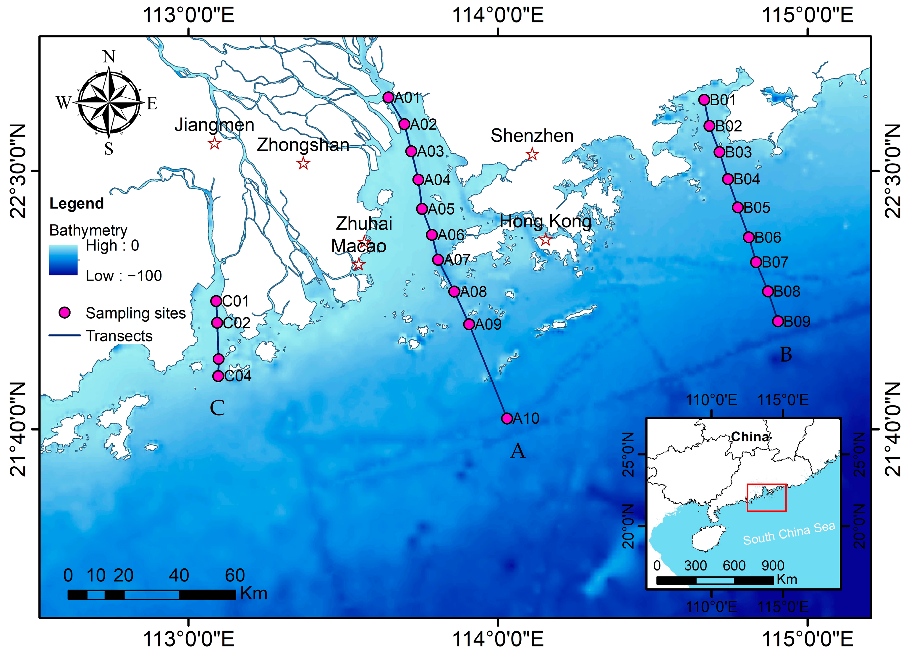
2.1. Study Area and Sampling

Optical and ecological environmental measurements were conducted in January 2020. The locations of the stations are shown in Figure 1. The stations were divided into three transects (A, B, and C). Transects A and C were located in the Lingdingyang Estuary and Huangmao Sea Estuary, respectively; both of them were estuaries of Pearl River, which is the largest water system in South China, with an annual mean runoff volume of 326 billion m³ [26]. Measurements were conducted at 10 stations and 4 stations, respectively, for transects A and C. Transect B was located in Daya Bay, and measurements were conducted at 9 stations. Facing the vast SCS, the research area has a subtropical and tropical monsoon climate, with an average temperature of 21–23 °C and a rainfall of more than 1500 mm each year [27]. The tide in the research area is irregular mixed semidiurnal tide, and the tidal range is up to 2 m. A total of 23 observations were conducted at all stations; for each station, a profiling optical measurement was conducted to obtain the water IOP (including coefficients of absorption, attenuation, scattering, and backscattering) and PSD data.

In this study, water samples were collected at each station using a Multi Water Sampler SlimLine 6 (Hydro-Bios, Altenholz, Germany) at different depths and filtered onboard. Near-surface water was collected for each station, and water samples in the vertical water column were collected at 5 m-depth intervals from the sea surface to the bottom for nearshore water (stations A1–A8, B1–B5, and C1–C4). To derive suspended particulate matter (SPM), the samples were filtered through pre-weighed and pre-combusted 47 mm GF/F filters (0.7 μm pore size), which were then frozen at −20 °C until analysis in the laboratory. The samples were subsequently dried (105 °C for 4 h) and weighed using a 0.0001 g resolution scale to calculate the SPM concentration [28,29].

2.2. Optical Properties Measurements

For the acquisition of seawater IOPs, measurements were conducted by means of an optical profiling package, which was formed using an AC-S spectral absorption and attenuation meter (WET Labs, Philomath, OR, USA), a BB9 backscattering instrument (WET Labs, USA), and an SBE37 CTD profiler (Sea-Bird Electronics, Bellevue, WA, USA). Data from the AC-S, BB9, and CTD instruments were collected using a DH-4 data handler (WET Labs, USA), which enabled simultaneous collection and storage; the data from different instruments can be merged subsequently based on time. The AC-S, BB9, and CTD instruments were calibrated by the manufacturer before the trip. When sampling, the profiling package was first placed into the surface waters for 3–4 min for environmental adaptation, then slowly down to 2–3 m above the bottom for a profile survey. After each observation, the instruments were brought to the deck and rinsed with pure water immediately. To avoid the impact of perturbations of the water column, only the downcast-measured data were used in the subsequent analyses.

The AC-S instrument was used to measure the absorption coefficient (a_pg(λ)) and attenuation coefficient (c_pg(λ)) of the constituents in seawater within 400–730 nm with intervals of approximately 4 nm. The raw data were initially corrected for the temperature and salinity following the AC-S protocol [30], and then the correction for the effect of tube scattering was performed following Sullivan et al. [31]. In addition, the entire absorption spectrum was normalized by subtracting the absorption at 715 nm [32]. The particle scattering (b_p(λ), in m⁻¹) was calculated as c_pg(λ) minus a_pg(λ) [33]. The backscattering measurements were conducted using the BB9 instrument with nine bands [21], and the particle backscattering coefficient (b_bp(λ), in m⁻¹) was obtained after the correction on raw BB9 data following the BB9 protocol [34]. b_p(λ) and b_bp(λ) were resampled at 5 m-depth intervals by averaging the data within a 0.5 m depth up and down, to match with the PSD and SPM datasets. Additionally, 532 nm was taken as a wavelength both for b_bp(λ) and b_p(λ) for the analysis, as it is closely related to the particle scattering properties and was less impacted by the absorption of pigments, and the wavelength dependency was not considered in this study.

2.3. PSD Acquisition

At each station, a LISST-200X Type-C particle size analyzer (Sequoia Scientific, Inc., Bellevue, WA, USA), which was mounted on the profiling package, was utilized for PSD measurements. Studies have shown that the LISST instrument is capable and widely used for in situ PSD measurements in marine water [22,35,36]. The LISST measures the volume concentration of suspended particles using particle diffraction through a collimated laser beam with a 670 nm wavelength [37]. At each observation, nonintrusive measurements were performed using 36 concentric ring-shaped detectors (i.e., 36 size bins), whose size spectrum was logarithmically placed within a size range of 1–500 µm, and the upper size was 1.18 times the lower size for each bin, with the exception of bin 1 [37]. To exclude the influence of background values for the subsequent analysis, the LISST was calibrated with Milli-Q water before the trip.

The particle volume concentration V(D) in the 36 size bins could be derived from the manufacturer-provided LISST-SOP software, which provided two particle shape models, and the random shape model was deemed more suitable for the natural waters [38]. The V(D) for each size bin was calculated using the random shape model in this study, and the total volume concentration (VC) within the measured size range could be derived by summing the V(D) of each size bin. It should be noted that the VC was calculated by summing the V(D) within the size bin of 4–33 (i.e., size range of 2.05–297 μm), as studies have shown that the data were not stable for the initial and final bins [21,38]. The particle number concentration N(D), which could be regarded as the number of spherical particles with the same diameter for each size bin, was derived by dividing V(D) by the volume of a sphere of the same diameter (Equation (1)). Additionally, the cross-sectional area concentration of particles (A(D), in m⁻¹) could be calculated using V(D) by assuming spherical particles (Equation (2)) [6]. The total number concentration (VC) and the total cross-sectional area concentration (AC) of particles were calculated by summarizing V(D) and A(D) separately. The equations are as follows:

$$\mathrm{N}\left(\mathrm{D}\right)=\frac{6\mathrm{V}\left(\mathrm{D}\right)}{{\mathsf{\pi }\mathrm{D}}^3}$$

(1)

$$\mathrm{A}\left(\mathrm{D}\right)=\frac{3\mathrm{V}\left(\mathrm{D}\right)}{2\mathrm{D}}$$

(2)

where D is the volume-equivalent spherical diameter, which is calculated by taking the geometric average of two boundary values of each size bin. The density function of the number concentration (N′(D), in count/m³μm), which represents the number of particles per unit volume of suspension normalized by the size bin width, could be calculated by dividing N(D) by the width of a given size bin ΔD (Equation (3)).

$${\mathrm{N}}^{\prime }\left(\mathrm{D}\right)=\frac{\mathrm{N}\left(\mathrm{D}\right)}{\Delta \mathrm{D}}$$

(3)

The median particle size D_v⁵⁰ and the power-law function (i.e., Junge distribution) were both used to characterize the PSD in this study, and the shape of PSD could be defined as below:

$${\mathrm{N}}^{\prime }\left(\mathrm{D}\right)={\mathrm{N}}^{\prime }\left({\mathrm{D}}_0\right){\left(\frac{\mathrm{D}}{{\mathrm{D}}_0}\right)}^{-\mathsf{\xi }}$$

(4)

where D₀ is the reference diameter and was determined to be 13 µm in this study; N’(D₀) is the density of the particle number with respect to the diameter of D₀; and ξ (dimensionless) is the PSD slope, which was obtained using least-square fitting on the log-transformed data of each sample [5].

2.4. Analysis of PSD with Respect to IOPs

In general, b_bp(λ) and b_p(λ) are most affected by the concentration of suspended particles; this is the reason that many studies have established the retrieval models for the mass concentration of SPM based on the scattering or backscattering properties [1,39]. However, b_bp(λ) is not always correlated well with SPM [17]; according to Mie’s theory, the b_bp(λ) is also affected by the backscattering efficiency (Q_bbe), the apparent density (ρ_a), and the mean diameter weighted by area (D_A), as shown by Equations (5)–(7):

$${\mathrm{b}}_{\mathrm{bp}}=\frac{3}{2}\frac{{\mathrm{Q}}_{\mathrm{bbe}}}{{\mathsf{\rho }}_{\mathrm{a}}{\mathrm{D}}_{\mathrm{A}}}\mathrm{SPM}$$

(5)

$${\mathsf{\rho }}_{\mathrm{a}}=\frac{\mathrm{SPM}}{\mathrm{VC}}$$

(6)

$${\mathrm{D}}_{\mathrm{A}}=\frac{\sum \mathrm{A}\left(\mathrm{D}\right)\mathrm{D}}{\mathrm{AC}}$$

(7)

where Q_bbe is the mean backscattering efficiency and is related to the proportion of organic and mineral particles [40]; this is beyond the scope of this study, so we did not consider it here. The D was within the 2.05 to 297 μm size range, which is consistent with the calculation of V(D). In the same way, Equation (5) can be written for b_p(λ) and the attenuation coefficient of particles c_p (in m⁻¹) in the wavelength of 670 nm, which was provided by the LISST instrument. The mass-specific particle backscattering coefficient, which is denoted as b_bp/SPM, has been used for particle size retrieval in several studies [10,19]. As we can see from Equation (5), b_bp/SPM is not only affected by particle size, but the density is also an impact factor to be considered.

The volume-specific particle backscattering coefficient (denoted as b_bp/VC), which can be derived by combining Equations (5) and (6), was investigated in this study as it can be scaled to the particle diameter size. The expression (Equation (8)) is as follows:

$${\mathrm{b}}_{\mathrm{bp}}/\mathrm{VC}=\frac{3}{2}\frac{{\mathrm{Q}}_{\mathrm{bbe}}}{{\mathrm{D}}_{\mathrm{A}}}$$

(8)

Similar to b_bp, Equation (8) can be written for b_p(λ) and c_p in the same way. To describe the correlations between PSD and IOPs, the b_bp, b_p, and c_p were all analyzed in this study.

2.5. Performance Matrix

Statistical analysis of the variables was performed in this study. In addition, regression analyses between different PSD parameters and the IOPs were also performed to show the relationships between them, and the goodness of fit was evaluated through the root mean squared error (RMSE) and mean absolute percentage error (MAPE) (Equations (9) and (10)).

$$\mathrm{RMSE}=\sqrt{\frac{1}{N}{\displaystyle \sum }_{i=1}^N{\left(y_i^{\prime }-y_i\right)}^2}$$

(9)

$$\mathrm{MAPE}=\frac{1}{N}{\displaystyle \sum }_{i=1}^N\left|\frac{y_i^{\prime }-y_i}{y_i}\right|$$

(10)

where $y_i^{\prime }$ represents the estimated value, y_i represents the observed value, and N is the number of samples.

3. Results

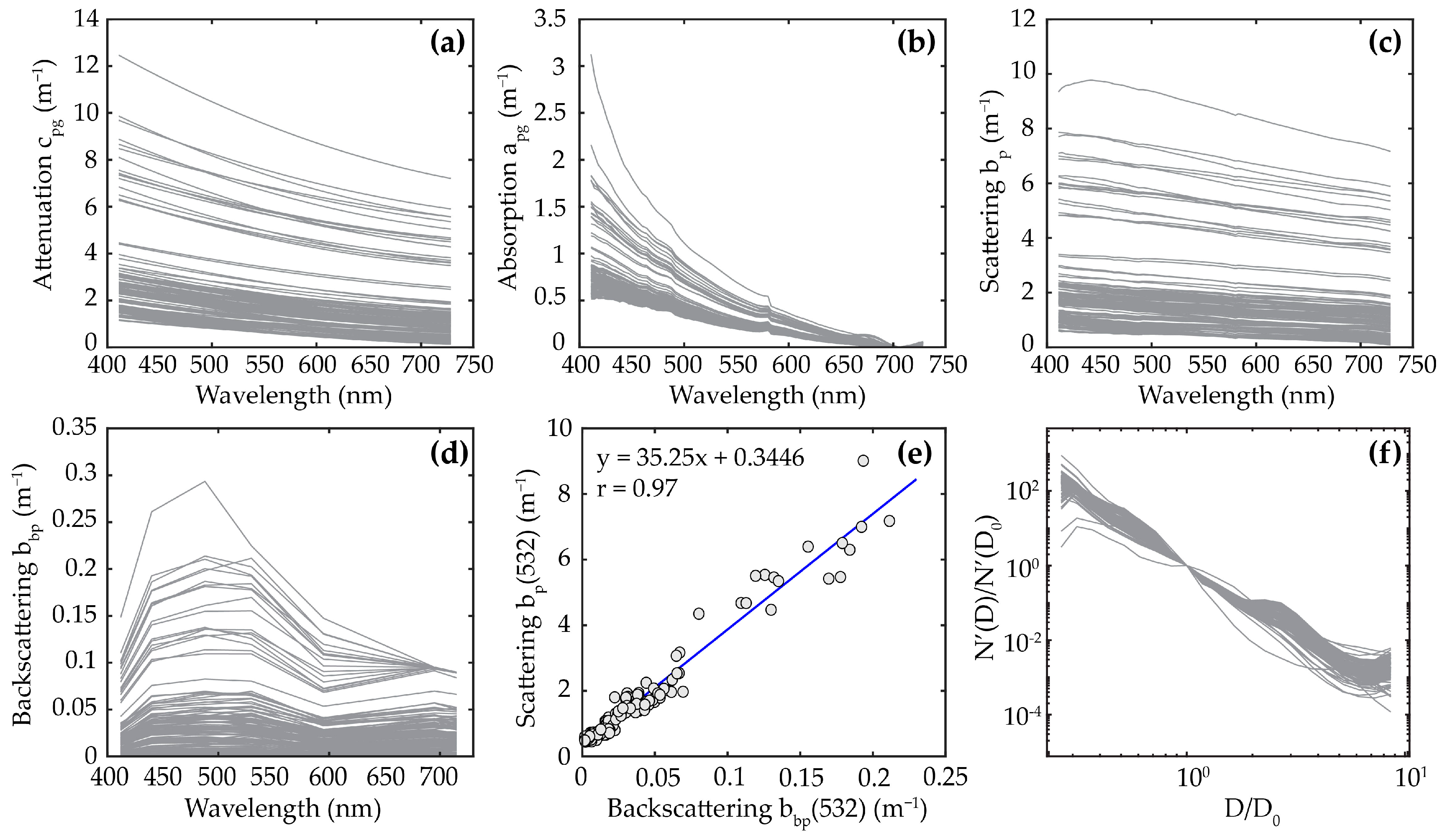
3.1. Inherent Optical Properties and PSD

The c_pg, a_pg, b_p, and b_bp with all wavelengths, which are provided by the AC-S and BB9 instruments, are shown in Figure 2a–d. The c_pg, a_pg, and b_p spectrums generally show decreasing trends with increasing wavelengths, while the b_bp spectrums show irregulated curves; besides, signal saturation occurs in the near-infrared region. Figure 2e shows a close relation between b_bp and b_p in 532 nm with a correlation coefficient of 0.97, which indicates the stability of particle backscattering ratio in the wavelength of 532 nm in the current study area. Hereafter, b_bp and b_p refer specifically to the values in 532 nm wavelength. Figure 2f shows the PSD described by the power-law model, which was generated by the regression analysis of N′(D)/N′(D₀) and D/D₀.

The measured and derived data (including IOPs, PSD parameters, and SPM) of the three transects are summarized in

Table 1. Descriptive statistics for IOPs (i.e., b_bp, b_p, and c_p), PSD parameters (i.e., NC, VC, AC, D_v⁵⁰, ξ, and D_A), SPM, specific IOPs (i.e., b_bp/SPM, b_p/SPM, c_p/SPM, b_bp/VC, b_p/VC, and c_p/VC), ρ_a, and the product of D_A and ρ_a. The mathematical statistics include the minimum, maximum, mean, standard deviation (SD), coefficient of variation (CV), and number of observations (N).

Variable	Units	Min	Max	Mean	SD	CV (%)	N
bbp	m−1	0.0017	0.2114	0.0419	0.0481	114.89	133
bp	m−1	0.45	9.01	1.80	1.67	93.21	133
cp	m−1	0.21	14.04	2.30	2.08	90.60	133
NC	1010 count m−3	0.21	11.90	1.70	1.86	109.57	133
VC	µL L−1	5.96	144.76	33.84	18.10	53.49	133
AC	m−1	0.38	3.47	0.79	0.53	66.76	133
Dv50	µm	41.60	263.02	227.35	37.08	16.31	133
ξ	none	2.61	3.74	3.07	0.19	6.16	133
SPM	g m−3	4.28	45.60	17.99	8.08	44.88	42
bbp/SPM	m2 g−1	0.0003	0.0156	0.0040	0.0033	83.06	42
bp/SPM	m2 g−1	0.03	0.73	0.17	0.13	71.80	42
cp/SPM	m2 g−1	0.04	1.13	0.22	0.19	87.16	42
bbp/VC	106 m−1	0.0001	0.0072	0.0012	0.0013	102.12	133
bp/VC	106 m−1	0.01	0.34	0.06	0.06	99.00	133
cp/VC	106 m−1	0.01	0.28	0.07	0.05	67.85	133
DA	μm	15.85	107.43	58.94	21.17	35.92	133
ρa	kg L−1	0.10	2.79	0.61	0.59	97.49	42
ρa DA	g m−2	5.37	86.18	28.96	16.25	56.09	42

. The data of IOPs and PSD parameters were matched at the same depth (i.e., 5 m interval from the water surface to the bottom for each station); in total, 133 samples were obtained for each parameter. As for the SPM and the parameters derived from the SPM, 42 samples were obtained separately after depth matching. The water investigated in our study shows relatively large variations for all parameters, especially for the IOPs (with CVs of 114.89%, 93.21%, and 90.6% for b_bp, b_p, and c_p, respectively), which indicates the uneven distribution of water components in the current research area. Correspondingly, the SPM, which ranged from 4.28 to 45.60 g m⁻³, with a CV of 44.88%, also showed a large variation of magnitude.

3.2. Variability of PSD

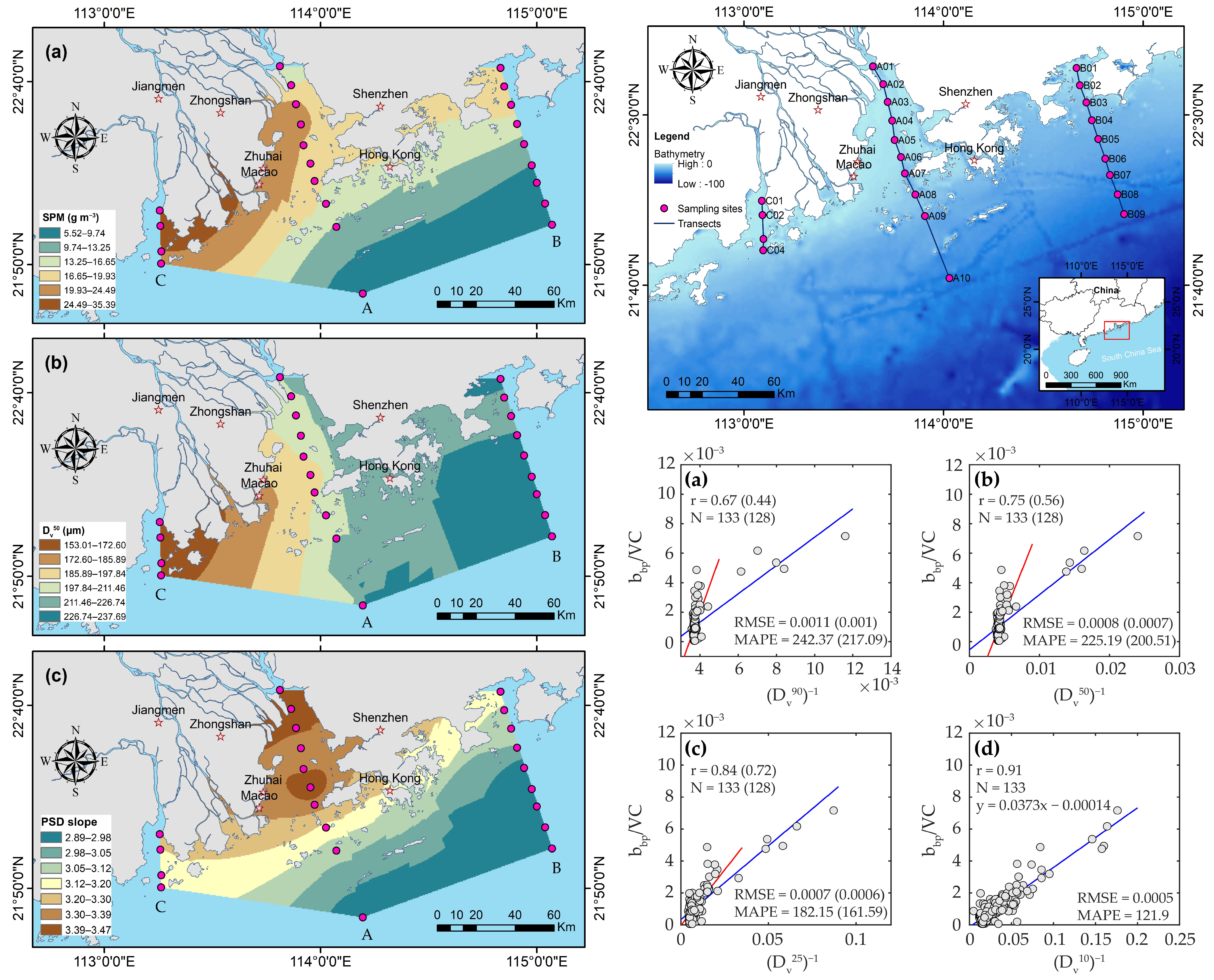
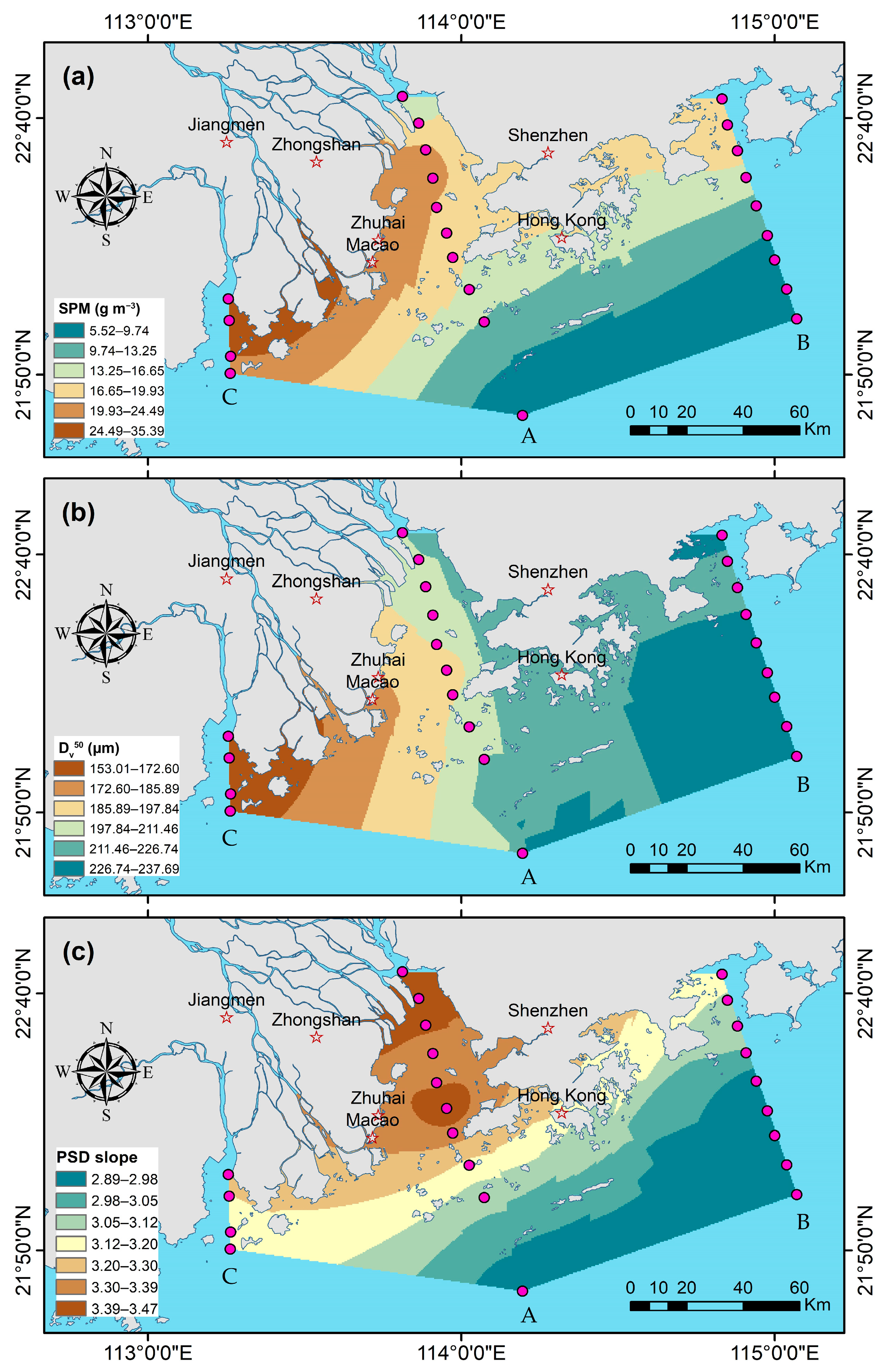
3.2.1. Variability of PSD in Surface Water

To analyze the variability of the PSD in the coastal waters of the northern SCS, the PSD data obtained from the surface water measurements of the three transects were used.

Figure 3 shows the spatial distribution of the D_v⁵⁰ and PSD slope, which was generated by a kriging interpolation with 23 stations, coupled with the spatial distribution of SPM for comparison. The D_v⁵⁰ showed a large spatial variability for the surface water of the research area, covering a range of 153.01 to 237.69 μm. Big differences occurred for the three transects, among which Transect B covered a D_v⁵⁰ range larger than 211.46 μm, while Transect C covered a D_v⁵⁰ range smaller than 172.6 μm, and D_v⁵⁰ of Transect A almost fell in between them. The D_v⁵⁰ in the eastern area showed relatively higher values than the western area; on the contrary, the SPM in the eastern area showed relatively lower values than the western area. The lower D_v⁵⁰ values were consistent with the higher SPM values; both were located in the water areas adjacent to river estuaries. The PSD slopes in the research area also showed relatively larger variability, with a range of 2.89 to 3.47. Additionally, as we can see, lower PSD slopes were most likely to exist in waters away from land, while relatively higher PSD slopes were found in the nearshore waters. Similar to the SPM distribution, the lowest PSD slopes occurred in the waters of Transect B and away from land.

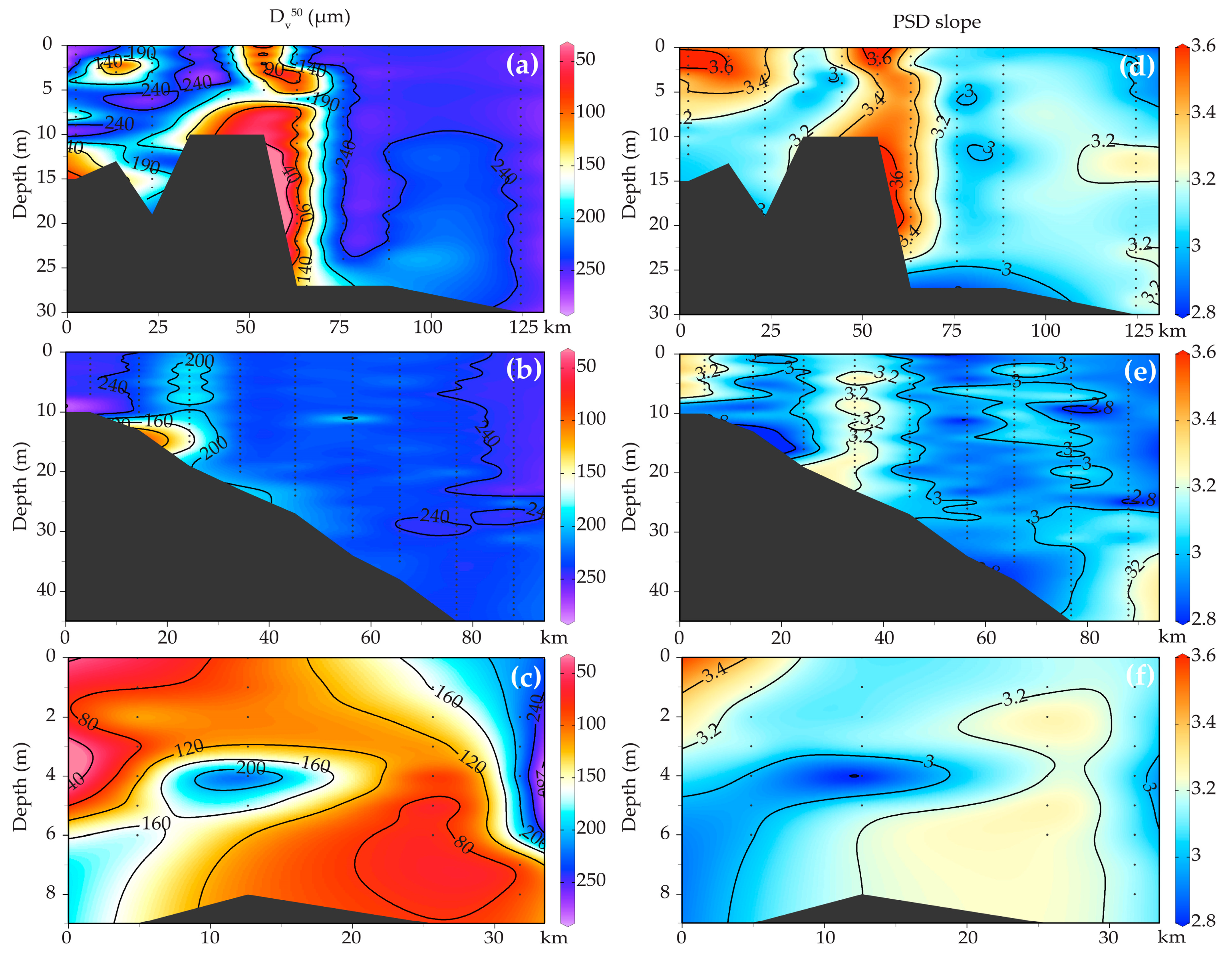
3.2.2. Vertical Variability of PSD

To further investigate the variability of PSD in the research area, the D_v⁵⁰ and PSD slope data, which were determined from vertical measurements for each station, were used. Figure 4 shows the vertical distributions of D_v⁵⁰ (Figure 4a–c) and PSD slope (Figure 4d–f) generated with a sampling interval of 1 m depth for the three transects. The D_v⁵⁰ in Transect A (Figure 4a) showed a big difference, with a range of 40 to 240 μm, and lower values appeared in the waters with a short distance to the shore. In addition, the differences between the upper and lower waters with different depths were obvious, and the lower values were more likely to appear at the bottom of shallow water. For D_v⁵⁰ in Transect B (Figure 4b), an area with lower values (<160 μm) appeared in the bottom water at a short distance from the shore, and larger values were more likely to appear in the waters far away from the shore. Most of the D_v⁵⁰ values in Transect C (Figure 4c), which is the shallowest of the three transects, were in a low range (80 to 120 μm). The PSD slopes in the three transects (Figure 4d–f) showed a similar pattern, but inversely to the D_v⁵⁰; in other words, larger PSD slopes are more likely to appear in the shallow waters at a short distance from the shore, and vice versa.

3.3. The Correlations between PSD and IOPs

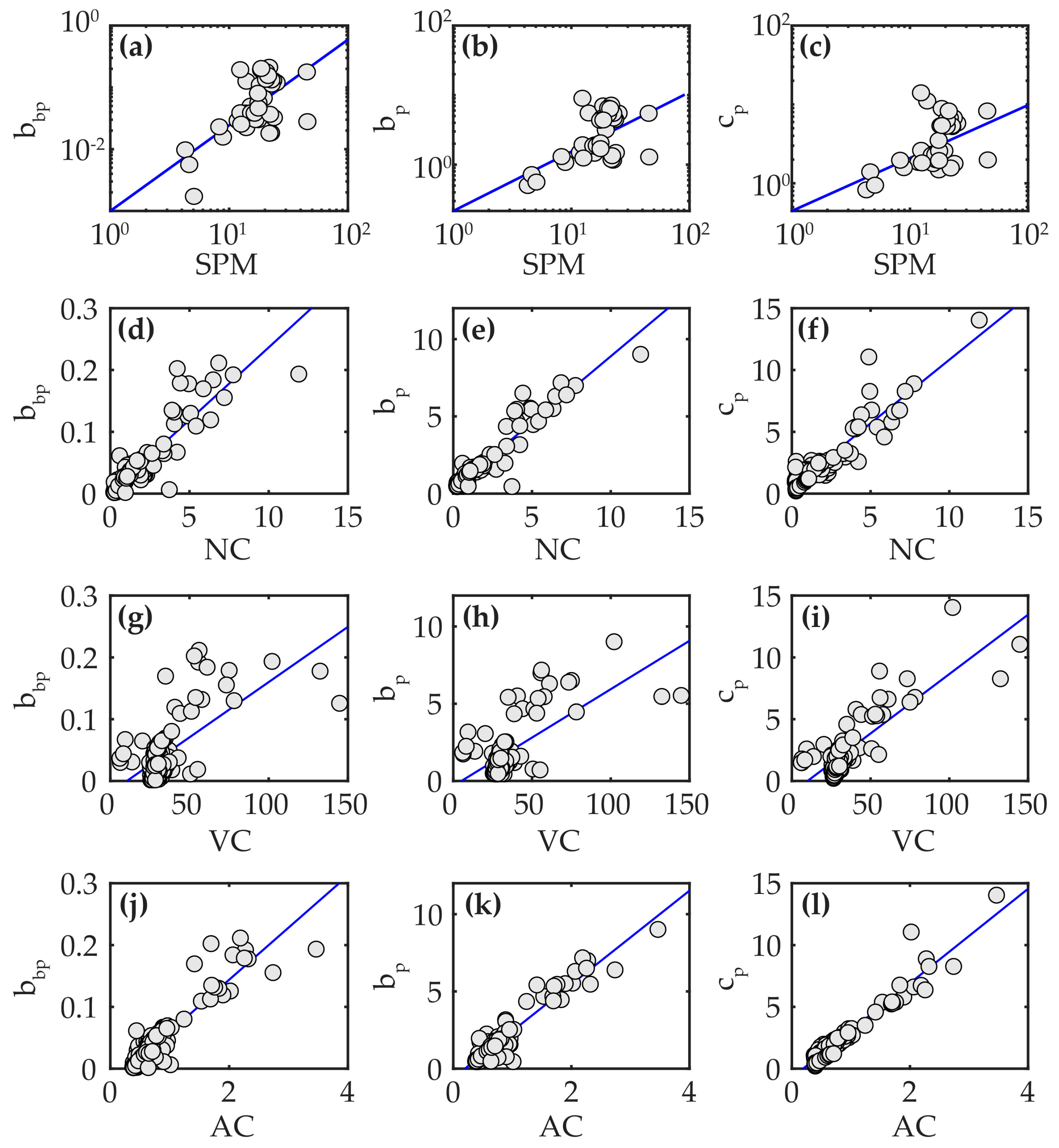
3.3.1. IOPs vs. SPM, VC, NC, and AC

In this study, the correlations between the IOPs (i.e., b_bp, b_p, and c_p) and the concentrations of suspended particles in mass, volume, number, and cross-sectional area (i.e., SPM, VC, NC, and AC) were analyzed to understand the impact factors of IOPs. A total of 133 data samples were collected for IOPs, and 42 data samples were collected for SPM. The scatter plots and best fit lines are shown in Figure 5.

Additionally, the corresponding correlation coefficients and goodness of fit, which were evaluated using the RMSE and MAPE, are shown in

Table 2. Correlations and regression analysis of IOPs (i.e., b_bp, b_p, and c_p) vs. the suspended particle concentrations in mass (SPM), number (NC), volume (VC), and cross-sectional area (AC). Slope (SE) and intercept (SE) are regression slope and intercept (SE, standard error of the regression slope and intercept), and N is the number of observations. All regressions were significant (F-test, p < 0.05).

IOPs	Concentrations	r	Slope (SE)	Incept (SE)	RMSE	MAPE	N
bbp	SPM	0.64	1.3853 (0.2646)	−6.9059 (0.7488)	0.094	102.71	42
	NC	0.91	0.0235 (0.0009)	0.002 (0.0024)	0.022	32.42	133
	VC	0.67	0.0018 (0.0002)	−0.0186 (0.0066)	0.036	107.05	133
	AC	0.92	0.0843 (0.0031)	−0.0246 (0.0029)	0.018	40.2	133
bp	SPM	0.55	0.854 (0.2039)	−1.5342 (0.5772)	12.44	153.14	42
	NC	0.95	0.8541 (0.0248)	0.3465 (0.0624)	0.53	15.86	133
	VC	0.68	0.0627 (0.0059)	−0.3236 (0.2280)	1.23	122.38	133
	AC	0.95	3.0294 (0.0838)	−0.5946 (0.0795)	0.5	21.41	133
cp	SPM	0.46	0.6712 (0.2032)	−0.8073 (0.5751)	15.17	160.02	42
	NC	0.92	1.028 (0.0383)	0.5496 (0.0963)	0.81	28.09	133
	VC	0.84	0.0961 (0.0055)	−0.9564 (0.2109)	1.14	88.98	133
	AC	0.97	3.8183 (0.0868)	−0.7189 (0.0823)	0.52	16.11	133

. All IOPs correlated well with both the area and number concentration, with correlation coefficients above 0.9 and relatively smaller RMSE and MAPE; this finding is inconsistent with previous studies [17,40]. A portion of variabilities of IOPs can also be explained by the volume concentration, with correlation coefficients above 0.67. However, all IOPs had poor correlations with SPM in a high value range; consequently, the accuracy was poor (r < 0.64).

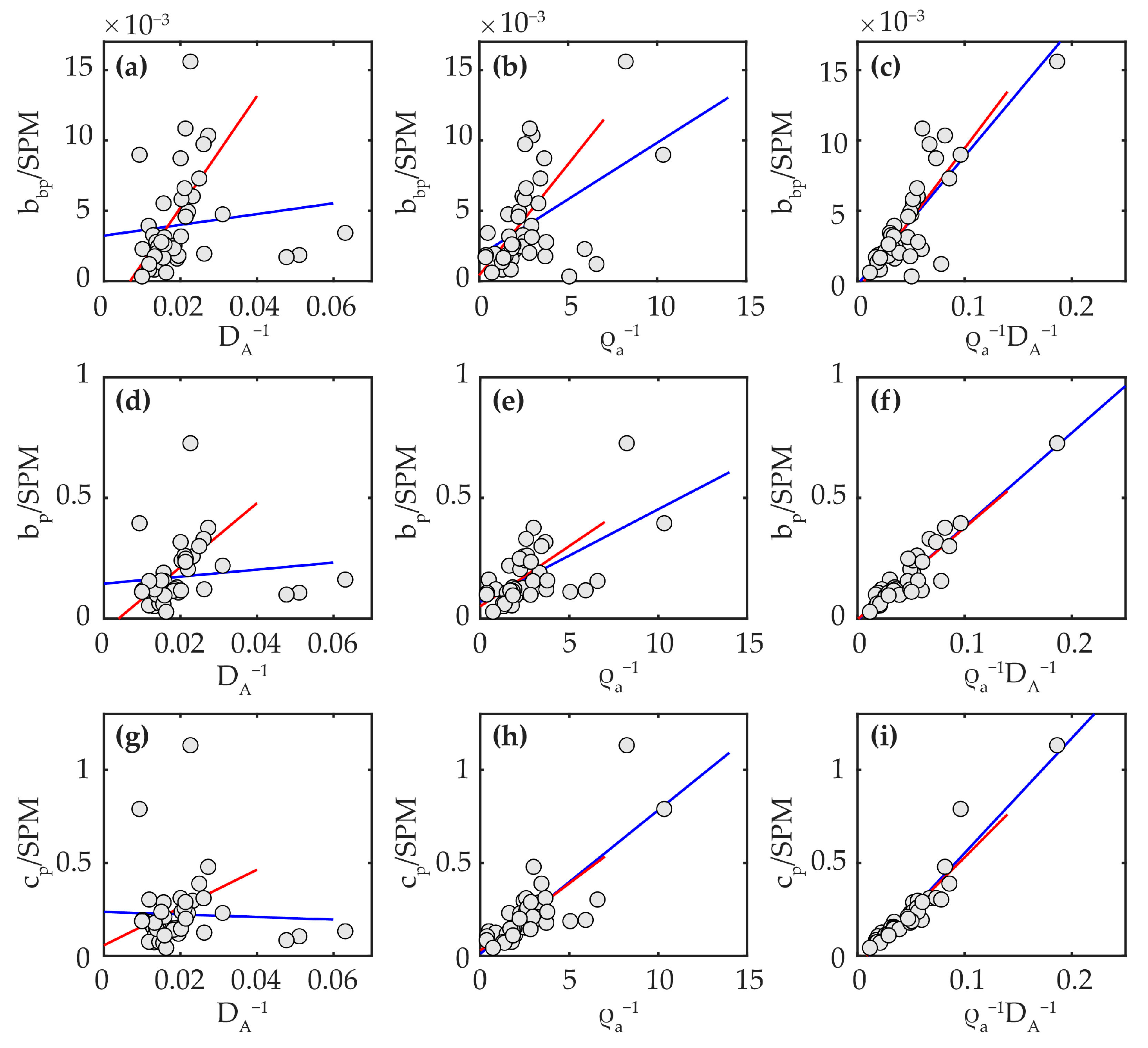
3.3.2. Mass-Specific IOPs vs. D_A, ρ_a, and ρ_aD_A

The correlations between the mass-specific IOPs (i.e., b_bp/SPM, b_p/SPM, and c_p/SPM) and the inverse of the mean particle diameter, D_A⁻¹; mean apparent density, ρ_a⁻¹; and the product of D_A⁻¹ and ρ_a⁻¹ were analyzed to understand the impact factors of mass-specific IOPs. To evaluate the correlations, the scatter plots and best fit lines are shown in Figure 6. A total of 42 data samples were used for each analysis. As we can see, there might be a trend line at the lower value region for some plots; therefore, the correlations and regressions for the low value samples were also analyzed.

The corresponding correlation coefficients and goodness of fit, which were evaluated using the RMSE and MAPE, are shown in

Table 3. Correlations and regression analysis of mass-specific backscattering (b_bp/SPM), scattering (b_p/SPM), and attenuation (c_p/SPM) vs. the inverse of mean particle diameter (D_A⁻¹), mean apparent density (ρ_a⁻¹), and the product of them (ρ_a⁻¹D_A⁻¹). The goodness of fit for regressions with all samples and partial samples (in italics) are given. Slope (SE) and intercept (SE) are regression slope and intercept (SE, standard error of the regression slope and intercept), N is the number of observations, and ns means not significant (i.e., p > 0.05).

IOPs	Concentrations	r	Slope (SE)	Incept (SE)	RMSE	MAPE	N	Significance
DA−1	bbp/SPM	0.13 0.56	0.0383 (0.0479) 0.3965 (0.0987)	0.0032 (0.0011) −0.0027 (0.0018)	0.003 0.003	116.5 81.60	42 38	ns
	bp/SPM	0.13 0.49	1.4487 (1.7993) 13.225 (3.8947)	0.1449 (0.0412) −0.0508 (0.0696)	0.123 0.112	68.78 55.66	42 38	ns
	cp/SPM	0.04 0.24	−0.6978 (2.8167) 10.1471 (6.7128)	0.2371 (0.0644) 0.0571 (0.1201)	0.192 0.193	70.67 64.3	42 38	ns ns
ρa−1	bbp/SPM	0.48 0.54	0.0008 (0.0002) 0.0016 (0.0004)	0.0018 (0.0008) 0.0004 (0.001)	0.003 0.002	114.75 66.61	42 37
	bp/SPM	0.61 0.54	0.0384 (0.0078) 0.05 (0.0133)	0.0691 (0.0275) 0.0504 (0.0308)	0.098 0.072	54.2 50.94	42 37
	cp/SPM	0.79 0.69	0.0772 (0.0094) 0.0721 (0.0126)	0.0117 (0.0318) 0.029 (0.0292)	0.117 0.068	38.31 35.34	42 37
ρa−1DA−1	bbp/SPM	0.82 0.74	0.091 (0.01) 0.1005 (0.0147)	−0.0002 (0.0005) −0.0006 (0.0007)	0.002 0.002	69.08 70.94	42 41
	bp/SPM	0.93 0.86	3.8812 (0.2368) 3.7956 (0.3532)	−0.0065 (0.0131) −0.003 (0.0169)	0.044 0.045	21.68 22.65	42 41
	cp/SPM	0.95 0.90	6.1716 (0.3045) 5.7807 (0.4468)	−0.0642 (0.0168) −0.0485 (0.0213)	0.057 0.057	18.69 15.88	42 41

. The scatter plots of mass-specific IOPs and D_A⁻¹ for either all samples or partial samples showed weak relationships (Figure 6a,d,g), with a poor fit (r < 0.6), and the correlation between the mass-specific IOPs and ρ_a⁻¹ was better than that of D_A⁻¹, with a better fit (r > 0.6 for b_p/SPM and c_p/SPM). Different from the former two, a large portion of variability for the IOPs can be explained by ρ_a⁻¹D_A⁻¹, which was consistent with the expression of Equation (5). These findings agree with those of previous studies [17]. Among the three IOPs, the b_p/SPM and c_p/SPM had a better fit, with a correlation coefficient of larger than 0.93; the RMSE was 0.045 and 0.051, and the MAPE was 19.01 and 31.66, respectively.

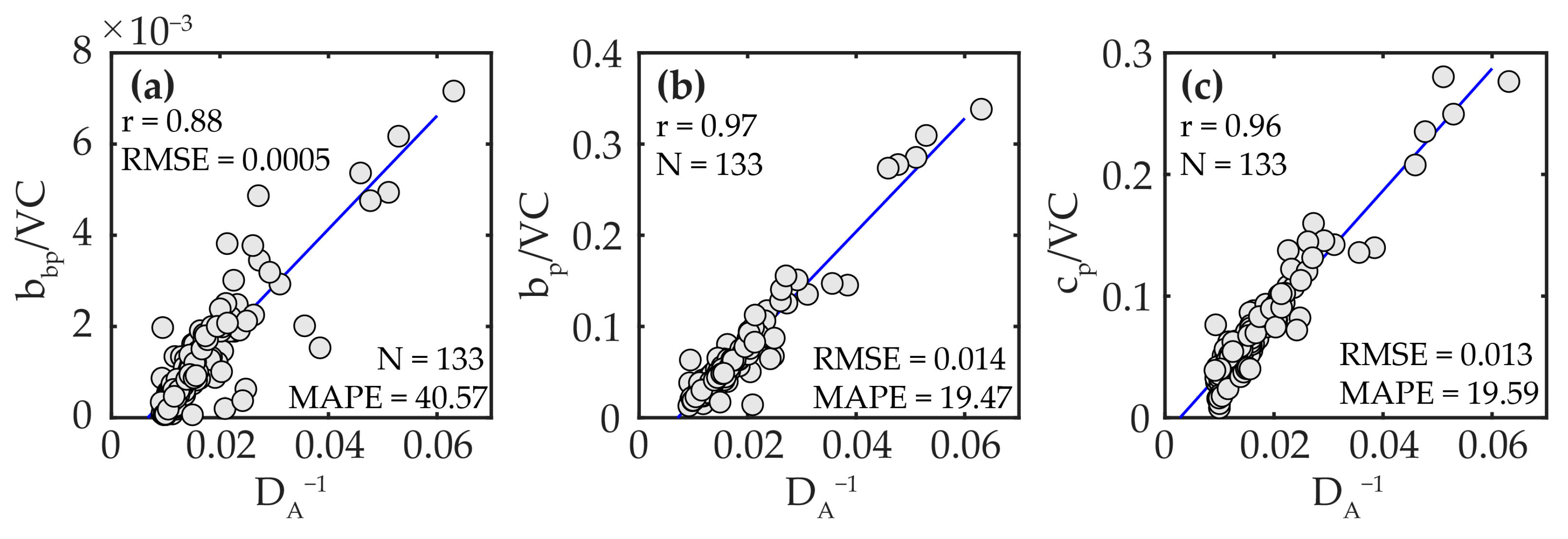
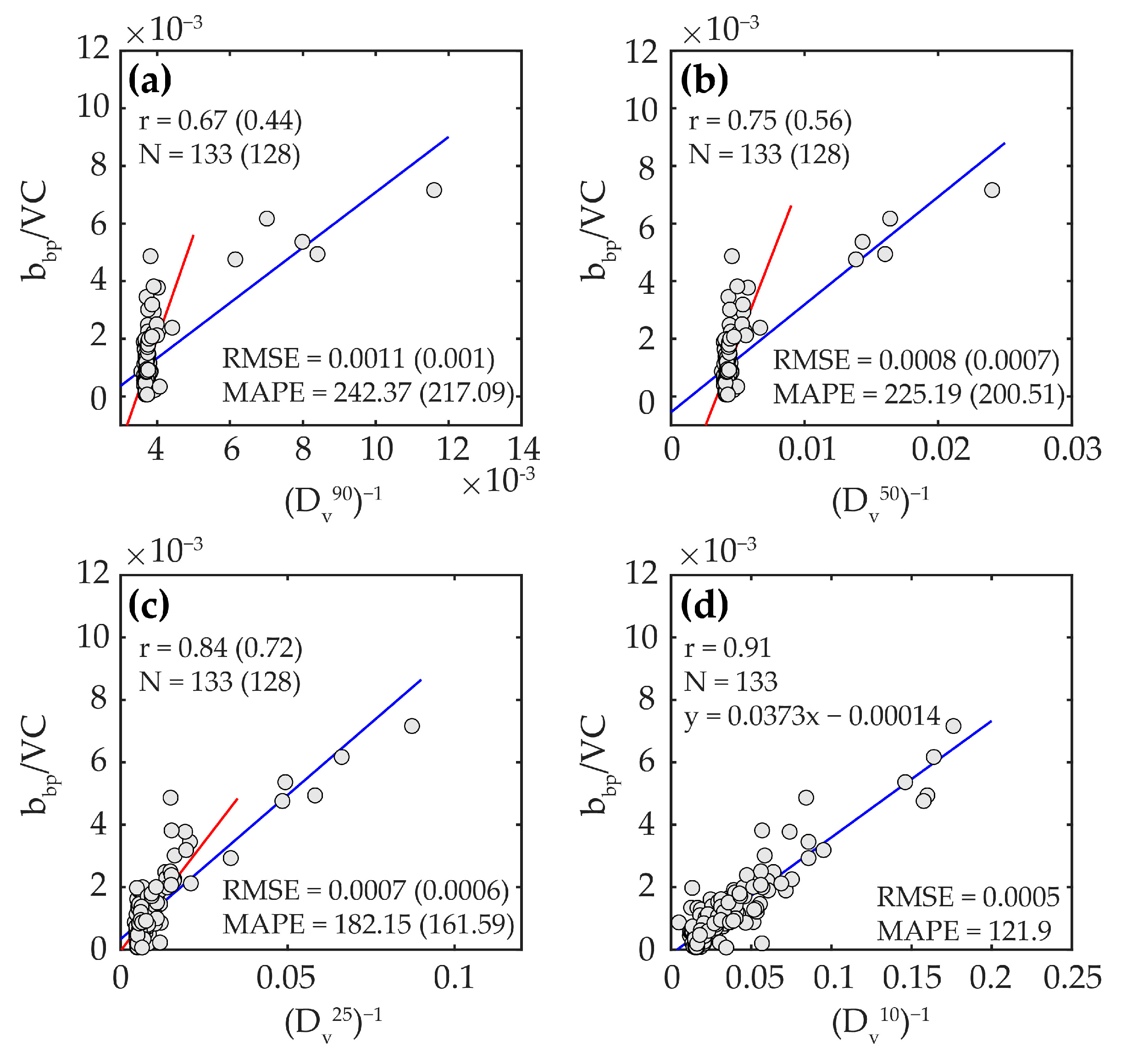
3.3.3. Volume-Specific IOPs vs. D_A and Percentile Diameters

As the Equation (8) presents, the mean particle size D_A may have a significant impact on the volume-specific IOPs; therefore, the correlations between the volume-specific IOPs (i.e., b_bp/VC, b_p/VC, and c_p/VC) and the inverse of the mean particle size D_A⁻¹ were investigated with 133 samples for each correlation in this study. The correlations and goodness of fit are shown in Figure 7. A strong correlation between the volume-specific IOPs and the mean particle size can be found, with a correlation coefficient larger than 0.88, which indicates that the PSD can explain most variabilities of volume-specific IOPs for the waters in the research area. This finding may provide a novel insight into retrieving the mean particle size from the b_bp or b_p, which were detected using the remote sensing method.

To further evaluate the correlations between volume-specific IOPs and PSD, the volume-specific backscattering b_bp/VC was investigated with respect to the correlations to PSD parameters. We used the percentile diameters for the cumulative size distributions, which corresponded to specific percentiles of the cumulative distribution of particle volume concentrations, to describe the PSD of each sample. A detailed description of the acquisition method for the percentile diameters can be found in Renolds et al. [6]. Figure 8 shows the correlation between b_bp/VC and the inverse of the 90th percentile diameter (D_v⁹⁰)⁻¹, the 50th percentile diameter (D_v⁵⁰)⁻¹, the 25th percentile diameter (D_v²⁵)⁻¹, and the 10th percentile diameter (D_v¹⁰)⁻¹. The D_v⁵⁰ is a frequently used PSD parameter and has been reported to have a significant effect on IOPs in previous studies [8,19]. However, the D_v⁵⁰ was not the most significant PSD parameter correlating with the volume-specific backscattering in the current study (Figure 8b). Instead, the D_v¹⁰ can explain the large portion of variability in volume-specific backscattering (Figure 8d), with a correlation coefficient, RMSE, and MAPE value of 0.97, 0.0005, and 112.9, respectively. These findings suggest that the variabilities of IOPs may be greatly impacted by particle size range; the choice of percentile diameters is important to evaluate the variabilities of IOPs.

4. Discussion

To explore the correlations between PSD and IOPs, we investigated the c_pg, a_pg, b_p, c_p, and b_bp in the coastal area of the northern SCS, in which these optical properties are not as well known. Unlike the open ocean, the optical properties in the coastal waters were complex and challenging to observe by the optical instruments such as AC-S and BB9. Extra care was needed when correcting these data as they were associated with various levels of uncertainties inherent in the measurement strategy [41]. In this study, each parameter covered about two orders of magnitude, which indicated the large variations in these properties. In addition, the spectrums of b_bp did not show the commonly presented exponential decay with increasing wavelength, which may result from the principal absorption associated with chlorophyll a and other major phytoplankton accessory pigments in blue bands [42]. Despite the spectral dependency, we only analyzed the b_bp and b_p in the wavelength of 532 nm, which was widely used in previous studies [17,33]. The close correlation between b_bp and b_p in 532 nm, which was shown in Figure 2e, indicated the consistency between the backscattering and scattering instruments, as well as the stable backscattering ratio in the study area.

As an indicator of the proportion of large particles and small particles, the D_v⁵⁰ was used in several representative studies. Bowers et al. reported a D_v⁵⁰ range of approximately 30 to 180 μm in the Irish Sea and adjacent waters [19], and Sun et al. found that the D_v⁵⁰ is within the range of 10.5 to 393.6 μm in the Bohai Sea and Yellow Sea [10]. The D_v⁵⁰ in our study was within the range of 41.60 to 263.02 μm, which is consistent with previous studies. The PSD slope was region-dependent and seemed to have a regular range according to that reported by previous studies: Roy et al. reported a range of 2 to 4.5 for global oceans [43]; Buonassissi and Dierssen found a range of within 2.7 to 4.7 for regional waters in the USA [22]; and Reynolds et al. investigated a global dataset and proposed a range of 2.65 to 4.49 [6]. The PSD slopes in our study are in agreement with these studies, with a range of 2.61 to 3.74.

The PSDs in both surface and vertical waters showed large variabilities in the current research area. For the surface distribution of D_v⁵⁰ (Figure 3b), small D_v⁵⁰ was most likely to appear in the water area adjacent to the estuaries of Pearl River, where a large amount of sediments are transported each year, and the fine sediment is the main mode [44]. This shows that small D_v⁵⁰ may indicate the predominance of inorganic terrestrial particles. Regarding the surface distribution of the PSD slope (Figure 3c), all three different transects showed that smaller particles were dominant in waters close to land, where the suspended particles were dominated by terrestrial inorganic sediments, and the lower PSD slopes in the offshore waters may indicate the predominance of large phytoplankton. These findings are in agreement with those reported by previous studies [4,5,45]. For the vertical variability of PSD (Figure 3), the lower D_v⁵⁰ values and higher PSD slopes were more likely to appear at the bottom of shallow water near the shore, which may result from the resuspension of fine particles from the bottom of shallow waters. On the contrary, higher D_v⁵⁰ values and lower PSD slopes appeared in the offshore waters, suggesting that the particles are dominated by larger phytoplankton, and less affected by resuspension.

To investigate the primary factors affecting the IOPs, we compared the correlation between the IOPs and the particle concentrations of SPM, NC, VC, and AC, of which the AC was the most relevant one, suggesting that the total cross-sectional area concentration of particles is the first considered factor for the variations of b_bp, b_p, and c_p. This finding is in agreement with that reported by Wang et al. [40]. Theoretically, IOPs are not only determined by particle concentrations—particle density and size are also important factors. Our results showed that the mass-specific IOPs were dominated by the product of the particle density and size; additionally, the density had a greater impact than size. Therefore, a large error may exist when estimating the particle size from the mass-specific IOPs. We changed the denominator of specific IOPs from mass to volume to exclude the impact of particle density, as shown in Equation (8), and the results showed that the volume-specific IOPs were greatly impacted by particle size. This result may provide the possibility to estimate the particle size using the volume-specific b_bp or b_p, which may be retrieved via the remote sensing method. Four percentile diameters of accumulated volume concentration, i.e., D_v⁹⁰, D_v⁵⁰, D_v²⁵, and D_v¹⁰, were used to further investigate the correlations between PSD and the volume-specific IOPs. Results showed that the D_v¹⁰ could better explain the volume-specific IOPs, which suggests an important potential contribution of inorganic particles to optical properties in the coastal waters with large riverine inputs and resuspension.

The observed PSD was dependent on the size range, which was provided by different instruments. We obtained the micron-sized PSD using the LISST instrument in the current study, while particles ranged from colloids of approximately 1 nm in size to large organisms of many meters long in the ocean [23]; therefore, particle size instruments with a wider range are needed to understand how PSD correlates with IOPs. Besides, the relations between the particle size and the volume-specific IOPs were established on the hypothesis of a spherical particle, and the composition is relatively stable in a region with limited area; therefore, to verify the reliability of these relations in different waters, long-term and vast PSD observations are needed.

5. Conclusions

In this study, we investigated the PSD variabilities and the correlations with IOPs in the coastal northern South China Sea based on in situ measurements. PSDs obtained from the research area demonstrated large differences both for the surface water with different locations and the water in the vertical planes of the transects. The PSD characteristics, which were described by the D_v⁵⁰ and PSD slope, indicated that a predominance of small particles was most likely to appear in the nearshore shallow water and the estuaries with large amounts of sediment discharge, and large phytoplankton might predominate in offshore waters. The correlations between PSD and the backscattering coefficient (b_bp), scattering coefficient (b_p), and attenuation coefficient (c_p) were also investigated; the first driving factor for the variations of b_bp, b_p, and c_p was particle concentration in the cross-sectional area, which is inconsistent with previous studies. In the current study, the mass-specific b_bp (b_bp/SPM), b_p (b_p/SPM), and c_p (c_p/SPM) were less impacted by the mean particle size (D_A) and mainly impacted by the product of D_A and particle apparent density (ρ_a). We found that D_A was strongly correlated with the volume-specific b_bp (b_bp/VC), b_p (b_p/VC), and c_p (c_p/VC); based on this, we further investigated the correlations between b_bp/VC and the percentile diameters. Finally, the D_v¹⁰ was proven to be the most relevant parameter to b_bp/VC. These findings suggest a potential retrieval method for PSD with optical particle properties, which may be determined by remote sensing observations.

References

1. Balasubramanian, S.V.; Pahlevan, N.; Smith, B.; Binding, C.; Schalles, J.; Loisel, H.; Gurlin, D.; Greb, S.; Alikas, K.; Randla, M.; et al. Robust algorithm for estimating total suspended solids (TSS) in inland and nearshore coastal waters. Remote Sens. Environ. 2020, 246, 111768. [Google Scholar] [CrossRef]
2. Runyan, H.; Reynolds, R.A.; Stramski, D. Evaluation of Particle Size Distribution Metrics to Estimate the Relative Contributions of Different Size Fractions Based on Measurements in Arctic Waters. J. Geophys. Res. Oceans 2020, 125, e2020JC016218. [Google Scholar] [CrossRef] [PubMed]
3. Nasiha, H.J.; Shanmugam, P.; Sundaravadivelu, R. Estimation of sediment settling velocity in estuarine and coastal waters using optical remote sensing data. Adv. Space Res. 2019, 63, 3473–3488. [Google Scholar] [CrossRef]
4. Xi, H.; Larouche, P.; Tang, S.; Michel, C. Characterization and variability of particle size distributions in Hudson Bay, Canada. J. Geophys. Res. Oceans 2014, 119, 3392–3406. [Google Scholar] [CrossRef]
5. Qiu, Z.; Sun, D.; Hu, C.; Wang, S.; Zheng, L.; Huan, Y.; Peng, T. Variability of Particle Size Distributions in the Bohai Sea and the Yellow Sea. Remote Sens. 2016, 8, 949. [Google Scholar] [CrossRef] [Green Version]
6. Reynolds, R.A.; Stramski, D. Variability in Oceanic Particle Size Distributions and Estimation of Size Class Contributions Using a Non-parametric Approach. J. Geophys. Res. Ocean. 2021, 126, e2021JC017946. [Google Scholar] [CrossRef]
7. Slade, W.H.; Boss, E. Spectral attenuation and backscattering as indicators of average particle size. Appl. Opt. 2015, 54, 7264–7277. [Google Scholar] [CrossRef]
8. Wozniak, S.; Stramski, D.; Stramska, M.; Reynolds, R.; Wright, V.M.; Miksic, E.Y.; Cichocka, M.; Cieplak, A. Optical variability of seawater in relation to particle concentration, composition, and size distribution in the near-shore marine environment at Imperial Beach, California. J. Geophys. Res. Ocean 2010, 115, C8. [Google Scholar] [CrossRef] [Green Version]
9. Reynolds, A.R.; Stramski, D.; Wright, M.V.; Woniak, B.S. Measurements and characterization of particle size distributions in coastal waters. J. Geophys. Res. Ocean. 2010, 115, C08024. [Google Scholar] [CrossRef]
10. Sun, D.; Qiu, Z.; Hu, C.; Wang, S.; Wang, L.; Zheng, L.; Peng, T.; He, Y. A hybrid method to estimate suspended particle sizes from satellite measurements over Bohai Sea and Yellow Sea. J. Geophys. Res. Ocean. 2016, 121, 6742–6761. [Google Scholar] [CrossRef]
11. Bader, H. The hyperbolic distribution of particle sizes. J. Geophys. Res. Earth Surf. 1970, 75, 2822–2830. [Google Scholar] [CrossRef]
12. Jonasz, M. Particle-size distributions in the Baltic. Tellus B Chem. Phys. Meteorol. 1983, 35, 346–358. [Google Scholar] [CrossRef]
13. Jonasz, M.; Fournier, G.R. Approximation of the size distribution of marine particles by a sum of log-normal functions. Limnol. Oceanogr. 1996, 41, 744–754. [Google Scholar] [CrossRef]
14. Risović, D. Two-component model of sea particle size distribution. Deep Sea Res. Part I: Oceanogr. Res. Pap. 1993, 40, 1459–1473. [Google Scholar] [CrossRef]
15. Junge, C.E. Air Chemistry and Radioactivity; Academic Press: New York, NY, USA, 1963. [Google Scholar]
16. Boss, E.; Twardowski, M.S.; Herring, S. Shape of the particulate beam attenuation spectrum and its inversion to obtain the shape of the particulate size distribution. Appl. Opt. 2001, 40, 4885–4893. [Google Scholar] [CrossRef]
17. Neukermans, G.; Loisel, H.; Mériaux, X.; Astoreca, R.; McKee, D. In situ variability of mass-specific beam attenuation and backscattering of marine particles with respect to particle size, density, and composition. Limnol. Oceanogr. 2011, 57, 124–144. [Google Scholar] [CrossRef] [Green Version]
18. Kostadinov, T.S.; Siegel, D.A.; Maritorena, S. Retrieval of the particle size distribution from satellite ocean color observations. J. Geophys. Res. Earth Surf. 2009, 114, C9. [Google Scholar] [CrossRef]
19. Bowers, D.G.; Binding, C.E.; Ellis, K.M. Satellite remote sensing of the geographical distribution of sus-pended particle size in an energetic shelf sea. Estuar Coast. Shelf Sci. 2007, 73, 457–466. [Google Scholar] [CrossRef]
20. van der Lee, E.; Bowers, D.; Kyte, E. Remote sensing of temporal and spatial patterns of suspended particle size in the Irish Sea in relation to the Kolmogorov microscale. Cont. Shelf Res. 2009, 29, 1213–1225. [Google Scholar] [CrossRef]
21. Wang, Z.; Hu, S.; Li, Q.; Liu, H.; Liao, X.; Wu, G. A Four-Step Method for Estimating Suspended Particle Size Based on In Situ Comprehensive Observations in the Pearl River Estuary in China. Remote Sens. 2021, 13, 5172. [Google Scholar] [CrossRef]
22. Buonassissi, C.J.; Dierssen, H.M. A regional comparison of particle size distributions and the power law approximation in oceanic and estuarine surface waters. J. Geophys. Res. Earth Surf. 2010, 115, C10. [Google Scholar] [CrossRef]
23. Jonasz, M.; Fournier, G. Light Scattering by Particles in Water: Theoretical and Experimental Foundations; Academic Press: Cambridge, MA, USA, 2007. [Google Scholar]
24. Mie, G. Beiträge zur Optik trüber Medien, speziell kolloidaler Metallösungen. Ann. Phys. 1908, 330, 377–445. [Google Scholar] [CrossRef]
25. Zhan, W.; Wu, J.; Wei, X.; Tang, S.; Zhan, H. Spatio-temporal variation of the suspended sediment concen-tration in the Pearl River Estuary observed by MODIS during 2003–2015. Cont. Shelf Res. 2019, 172, 22–32. [Google Scholar] [CrossRef]
26. Xu, W.; Yan, W.; Li, X.; Zou, Y.; Chen, X.; Huang, W.; Miao, L.; Zhang, R.; Zhang, G.; Zou, S. Antibiotics in riverine runoff of the Pearl River Delta and Pearl River Estuary, China: Concentrations, mass loading and ecological risks. Environ. Pollut. 2013, 182, 402–407. [Google Scholar] [CrossRef]
27. Su, Q.; Li, Z.; Li, G.; Zhu, D.; Hu, P. Application of the Coastal Hazard Wheel for Coastal Multi-Hazard Assessment and Management in the Guang-Dong-Hongkong-Macao Greater Bay Area. Sustainability 2021, 13, 12623. [Google Scholar] [CrossRef]
28. Wang, Z.; Kawamura, K.; Sakuno, Y.; Fan, X.; Gong, Z.; Lim, J. Retrieval of Chlorophyll-a and Total Sus-pended Solids Using Iterative Stepwise Elimination Partial Least Squares (ISE-PLS) Regression Based on Field Hy-perspectral Measurements in Irrigation Ponds in Higashihiroshima, Japan. Remote Sens. 2017, 9, 264. [Google Scholar] [CrossRef] [Green Version]
29. Zhang, Y.; Shi, K.; Zhou, Y.; Liu, X.; Qin, B. Monitoring the river plume induced by heavy rainfall events in large, shallow, Lake Taihu using MODIS 250m imagery. Remote Sens. Environ. 2015, 173, 109–121. [Google Scholar] [CrossRef]
30. Wet Labs. AC Meter Protocol Document (Revision Q); Wet Labs, Inc.: Philomath, OR, USA, 2011. [Google Scholar]
31. Sullivan, J.M.; Twardowski, M.S.; Zaneveld, J.R.V.; Moore, C.M.; Barnard, A.H.; Donaghay, P.L.; Rhoades, B. Hyperspectral temperature and salt dependencies of absorption by water and heavy water in the 400–750 nm spectral range. Appl. Opt. 2006, 45, 5294–5309. [Google Scholar] [CrossRef] [Green Version]
32. Lin, J.; Cao, W.; Wang, G.; Zhou, W.; Sun, Z.; Zhao, W. Inversion of bio-optical properties in the coastal upwelling waters of the northern South China Sea. Cont. Shelf Res. 2014, 85, 73–84. [Google Scholar] [CrossRef]
33. Martinez-Vicente, V.; Land, P.E.; Tilstone, G.H.; Widdicombe, C.; Fishwick, J.R. Particulate scattering and backscattering related to water constituents and seasonal changes in the Western English Channel. J. Plankton Res. 2010, 32, 603–619. [Google Scholar] [CrossRef]
34. Wet Labs. Scattering Meter ECO BB9 User’s Guide (Revision L); Wet Labs, Inc.: Philomath, OR, USA, 2013. [Google Scholar]
35. Huang, J.; Chen, X.; Jiang, T.; Yang, F.; Chen, L.; Yan, L. Variability of particle size distribution with respect to inherent optical properties in Poyang Lake, China. Appl. Opt. 2016, 55, 5821–5829. [Google Scholar] [CrossRef] [PubMed]
36. Lei, S.; Wu, D.; Li, Y.; Wang, Q.; Huang, C.; Liu, G.; Zheng, Z.; Du, C.; Mu, M.; Xu, J.; et al. Remote sensing monitoring of the suspended particle size in Hongze Lake based on GF-1 data. Int. J. Remote Sens. 2018, 40, 3179–3203. [Google Scholar] [CrossRef]
37. LISST-200X Particle Size Analyzer: User’s Manual (Version 1.3B); Sequoia Scientific, Inc.: Bellevue, WA, USA, 2018.
38. Agrawal, Y.C.; Whitmire, A.; Mikkelsen, O.A.; Pottsmith, H.C. Light scattering by random shaped particles and consequences on measuring suspended sediments by laser diffraction. J. Geophys. Res. Ocean 2008, 113, C4. [Google Scholar] [CrossRef] [Green Version]
39. Kratzer, S.; Kyryliuk, D.; Brockmann, C. Inorganic suspended matter as an indicator of terrestrial influence in Baltic Sea coastal areas—Algorithm development and validation, and ecological relevance. Remote Sens. Environ. 2020, 237, 111609. [Google Scholar] [CrossRef]
40. Wang, S.; Qiu, Z.; Sun, D.; Shen, X.; Zhang, H. Light beam attenuation and backscattering properties of particles in the Bohai Sea and Yellow Sea with relation to biogeochemical properties. J. Geophys. Res. Oceans 2016, 121, 3955–3969. [Google Scholar] [CrossRef] [Green Version]
41. Lin, J.; Lee, Z.; Ondrusek, M.; Liu, X. Hyperspectral absorption and backscattering coefficients of bulk wa-ter retrieved from a combination of remote-sensing reflectance and attenuation coefficient. Opt. Express 2018, 26, A157–A177. [Google Scholar] [CrossRef]
42. Reynolds, R.A.; Stramski, D.; Neukermans, G. Optical backscattering by particles in Arctic seawater and relationships to particle mass concentration, size distribution, and bulk composition. Limnol. Oceanogr. 2016, 61, 1869–1890. [Google Scholar] [CrossRef] [Green Version]
43. Roy, S.; Sathyendranath, S.; Bouman, H.; Platt, T. The global distribution of phytoplankton size spectrum and size classes from their light-absorption spectra derived from satellite data. Remote Sens. Environ. 2013, 139, 185–197. [Google Scholar] [CrossRef]
44. Ye, F.; Huang, X.; Zhang, D.; Tian, L.; Zeng, Y. Distribution of heavy metals in sediments of the Pearl River Estuary, Southern China: Implications for sources and historical changes. J. Environ. Sci. 2012, 24, 579–588. [Google Scholar] [CrossRef]
45. Lei, S.; Xu, J.; Li, Y.; Li, L.; Lyu, H.; Liu, G.; Chen, Y.; Lu, C.; Tian, C.; Jiao, W. A semi-analytical algorithm for deriving the particle size distribution slope of turbid inland water based on OLCI data: A case study in Lake Hongze. Environ. Pollut. 2020, 270, 116288. [Google Scholar] [CrossRef]
Figure 1. Study area and sampling stations; the letter of each station name indicates the transect for field sampling (i.e., Transect A, B, and C).
Remotesensing 14 02881 g001
Figure 2. The measured IOPs and PSD parameters. (ad) cpg, apg, bp, and bbp with all provided wavelengths. (e) The correlation between bp and bbp in 532 nm. (f) The measured PSD described by the power-law model. The blue line is the best-fit line.
Remotesensing 14 02881 g002
Figure 3. Surface distributions for (a) SPM, (b) Dv50, and (c) PSD slope. The pink dots indicate the stations in three transects (labeled with A, B, and C).
Remotesensing 14 02881 g003
Figure 4. Left panel: vertical distribution of Dv50 for (a) Transect A, (b) Transect B, and (c) Transect C; right panel: vertical distribution of PSD slope for (d) Transect A, (e) Transect B, and (f) Transect C. The horizontal axis indicates the distance 5 km away from the first station of each transect, the black dots represent the sampling points, and the black shading indicates the bathymetry in each subfigure.
Remotesensing 14 02881 g004
Figure 5. Correlations between the IOPs (i.e., bbp, bp, and cp) and the concentrations of suspended particles in mass, volume, number, and area (i.e., SPM, VC, NC, and AC). (ac) SPM vs. bbp, bp, and cp; (df) NC vs. bbp, bp, and cp; (gi) VC vs. bbp, bp, and cp; (jl) AC vs. bbp, bp, and cp. The blue line is the best-fit line in each subplot.
Remotesensing 14 02881 g005
Figure 6. Correlations between the mass-specific backscattering (bbp/SPM), scattering (bp/SPM), and attenuation (cp/SPM) vs. the inverse of mean particle diameter (DA−1), mean apparent density (ρa−1), and the product of them (ρa−1DA−1). (ac) bbp/SPM vs. DA−1, ρa−1, and ρa−1DA−1; (df) bp/SPM vs. DA−1, ρa−1, and ρa−1DA−1; (gi) cp/SPM vs. DA−1, ρa−1, and ρa−1DA−1. The blue line is the best-fit line for all samples and the red line is the best-fit line for partial samples (x < 0.03 for (a,d,g); x < 5 for (b,e,h); x < 0.1 for (c,f,i)) in each subplot.
Remotesensing 14 02881 g006
Figure 7. Correlations between the volume-specific IOPs and the inverse of mean particle size (DA−1). (a) bbp/VC vs. DA−1; (b) bp/VC vs. DA−1; (c) cp/VC vs. DA−1. The blue line is the best-fit line in each subplot.
Remotesensing 14 02881 g007
Figure 8. Correlations between the volume-specific backscattering bbp/VC vs. (a) the inverse of the 90th percentile diameter (Dv90)−1; (b) the 50th percentile diameter (Dv50)−1; (c) the 25th percentile diameter (Dv25)−1; (d) the 10th percentile diameter (Dv10)−1. The blue line is the linear fit for all data displayed in each subplot. The red line is the linear fit for partial data ((Dv90)−1 < 0.005, (Dv50)−1 < 0.01, and (Dv25)−1 < 0.05), and the accuracies are shown between brackets.
Remotesensing 14 02881 g008