
A New Analysis Method for Magnetic Disturbances Possibly Related to Earthquakes Observed by Satellites


Abstract
:1. Introduction
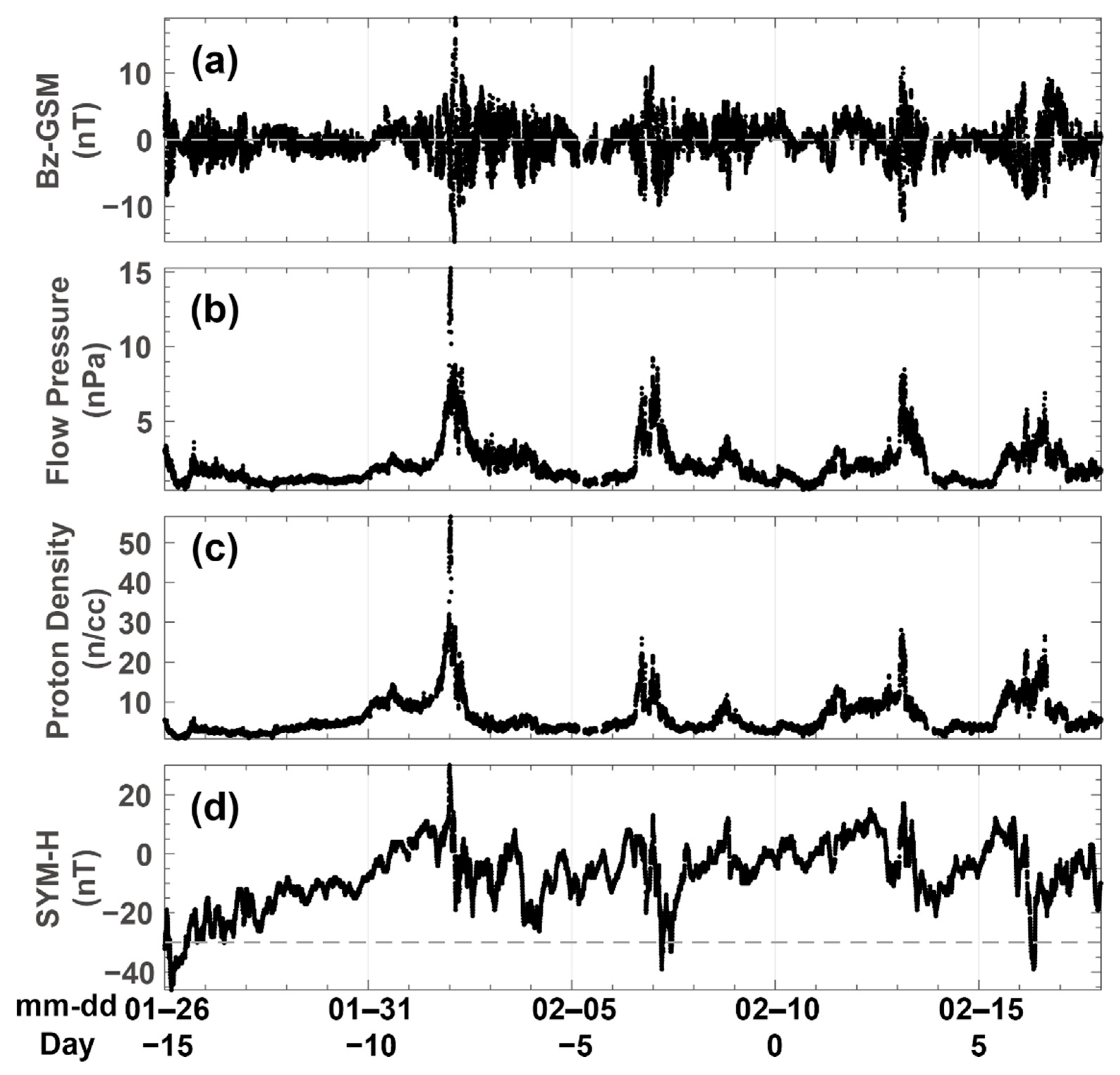
2. Data and Methods
3. Results
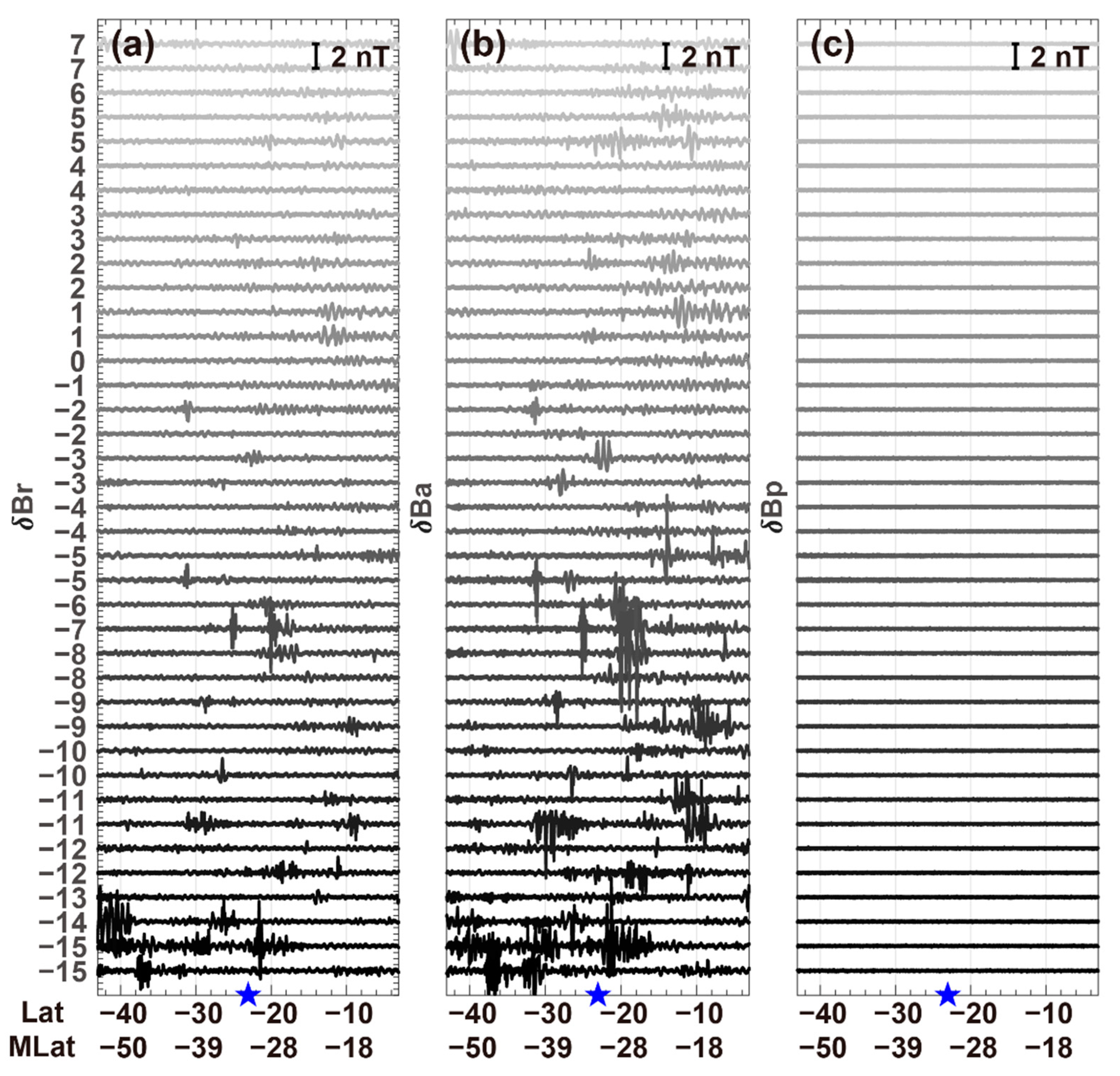
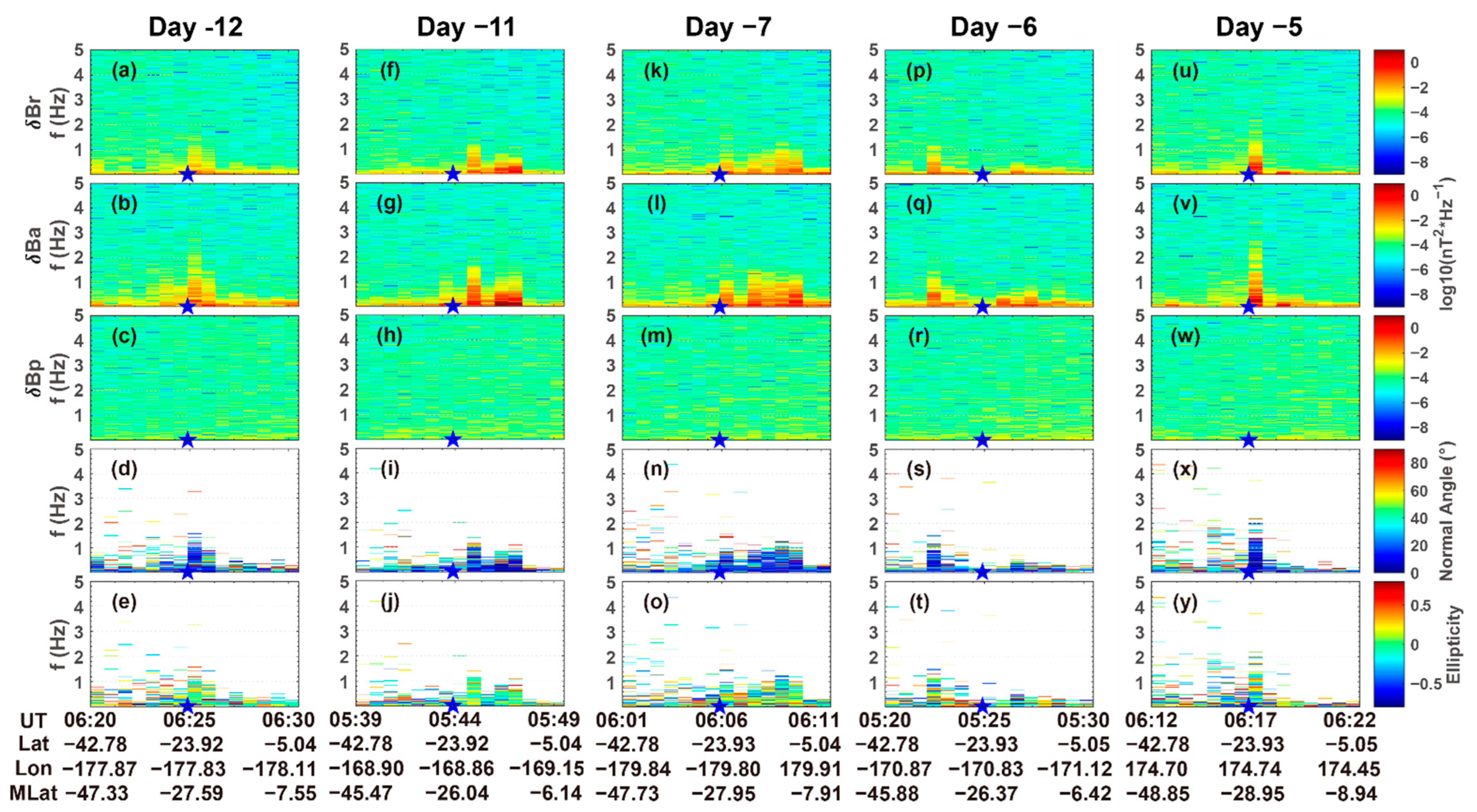
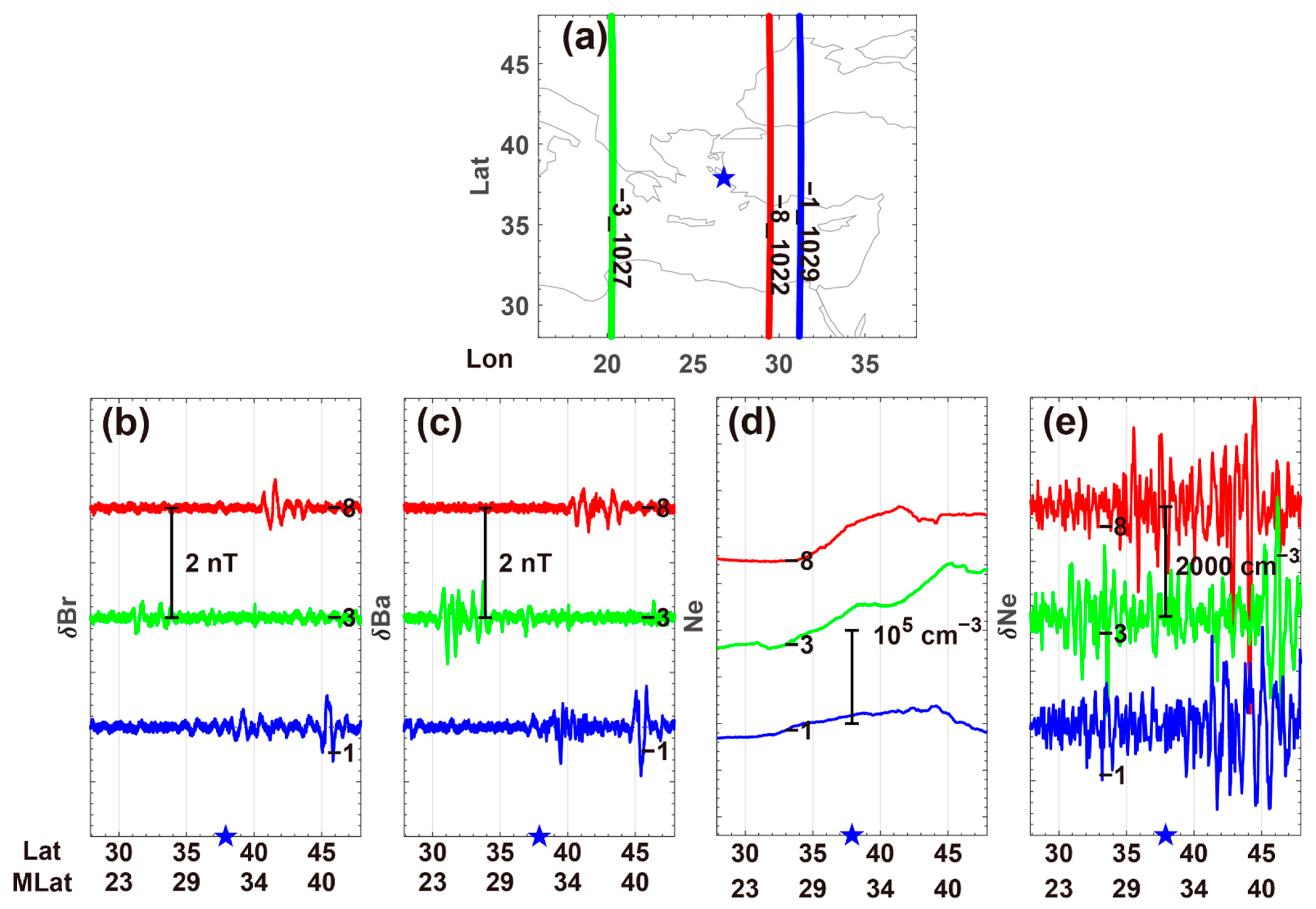
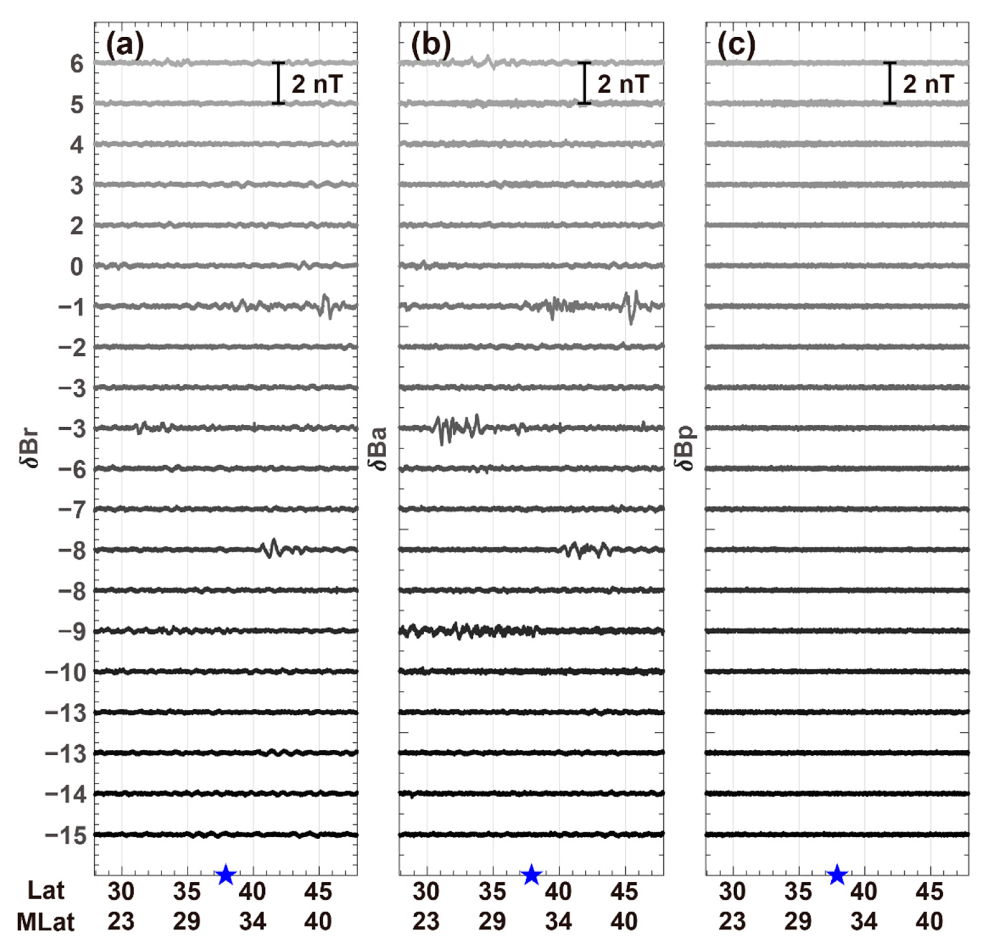
3.1. Overview of Magnetic Disturbances Observed by Swarm B
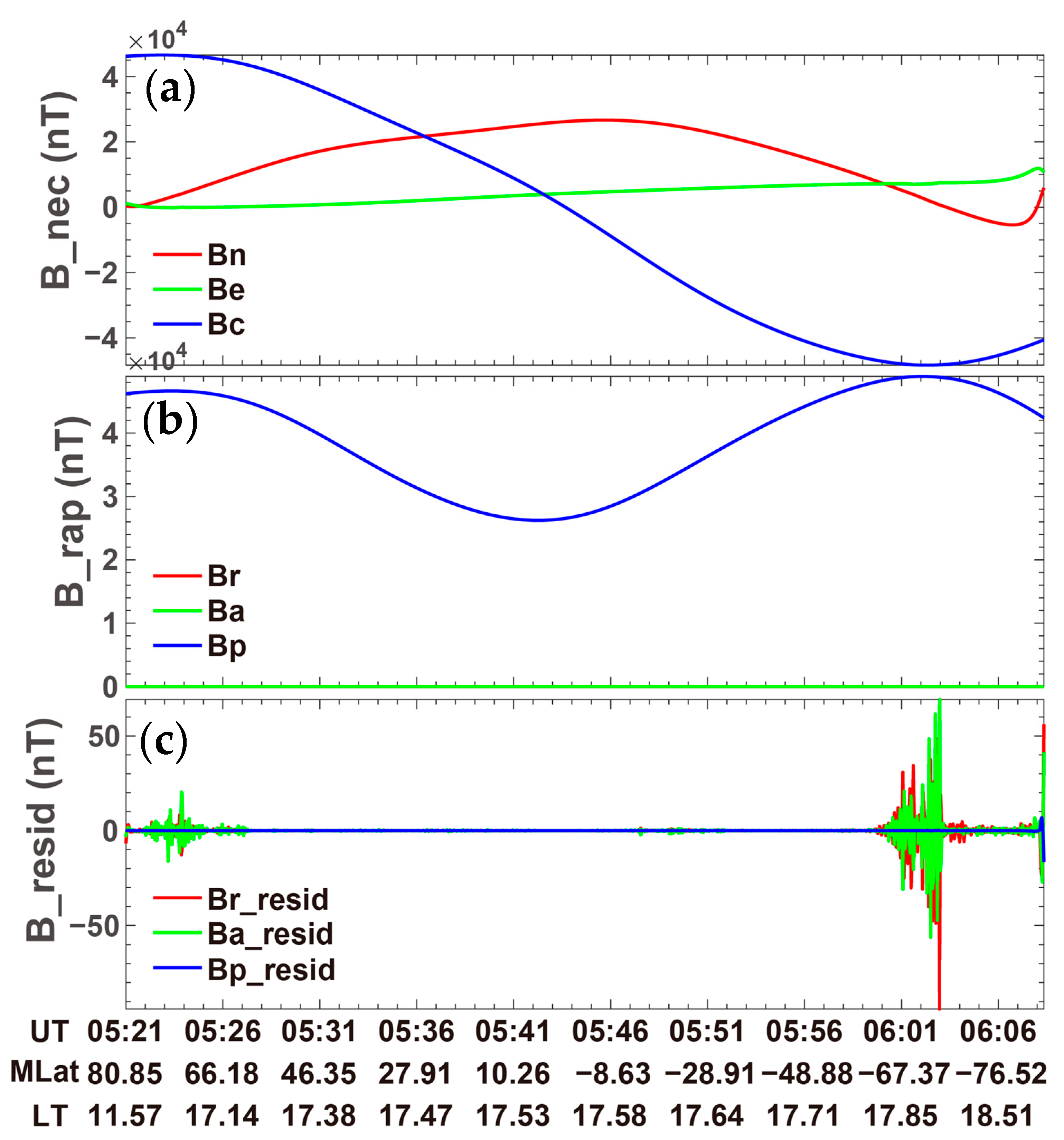
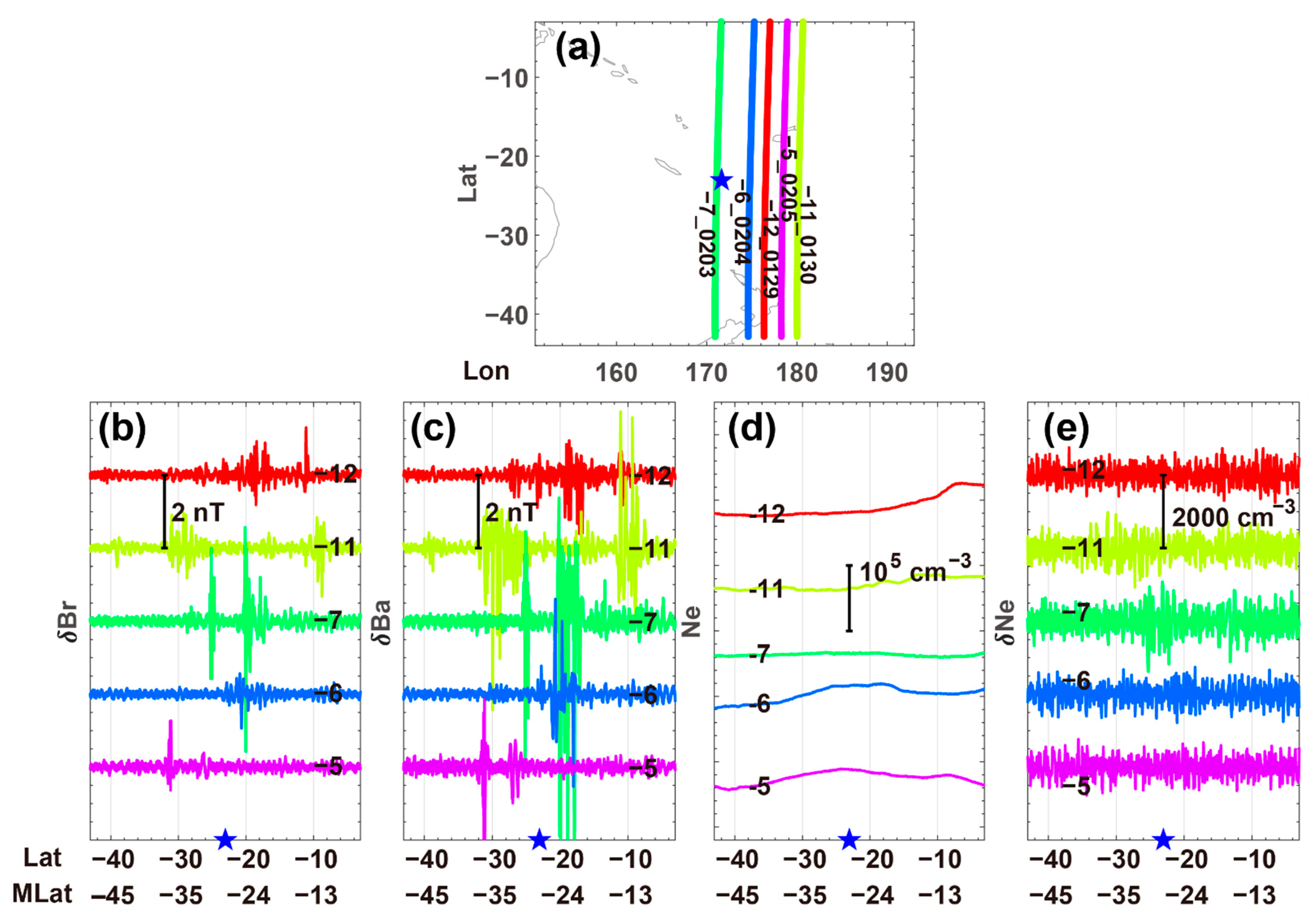
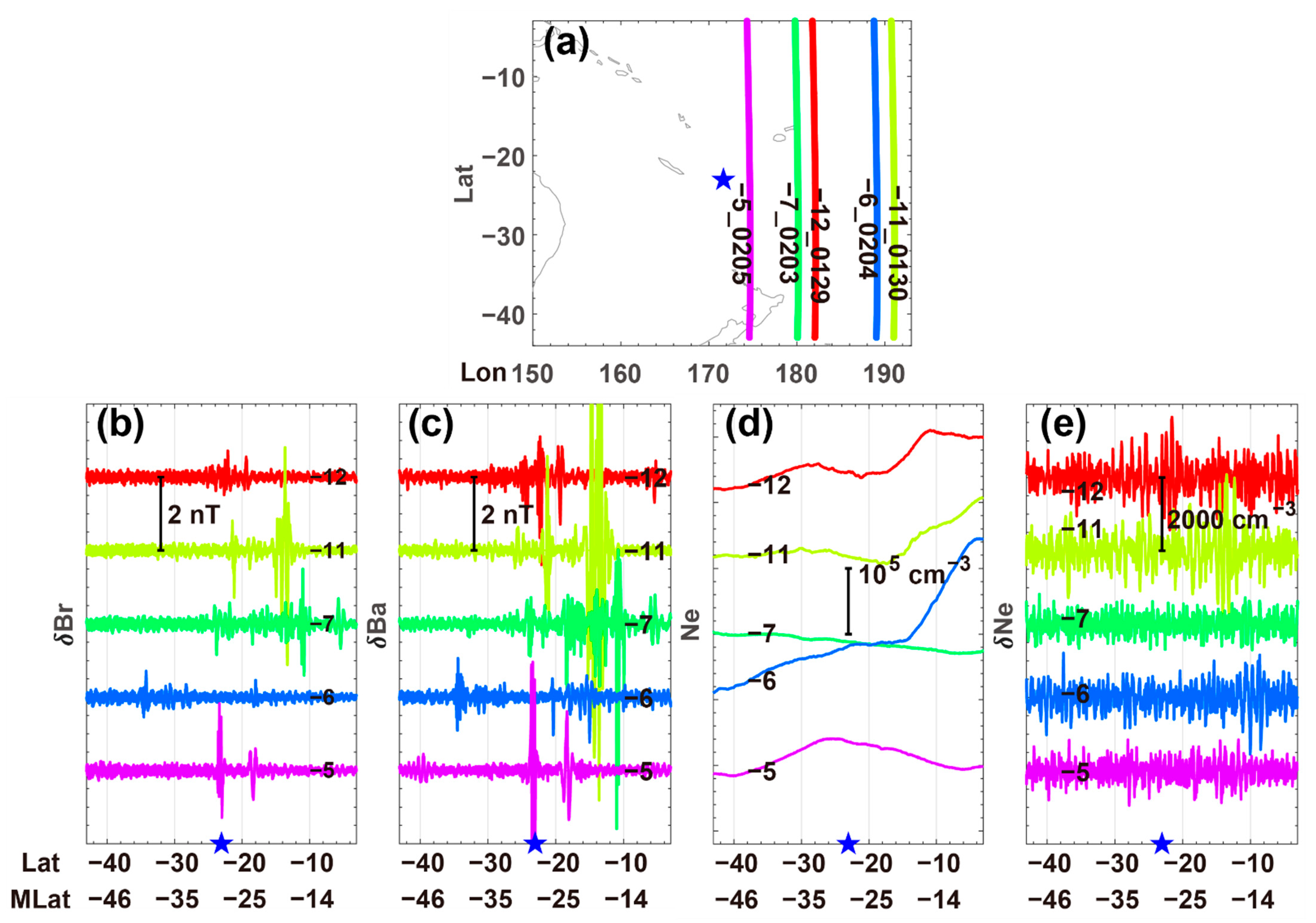
3.2. Magnetic Disturbances Observed by Swarm A
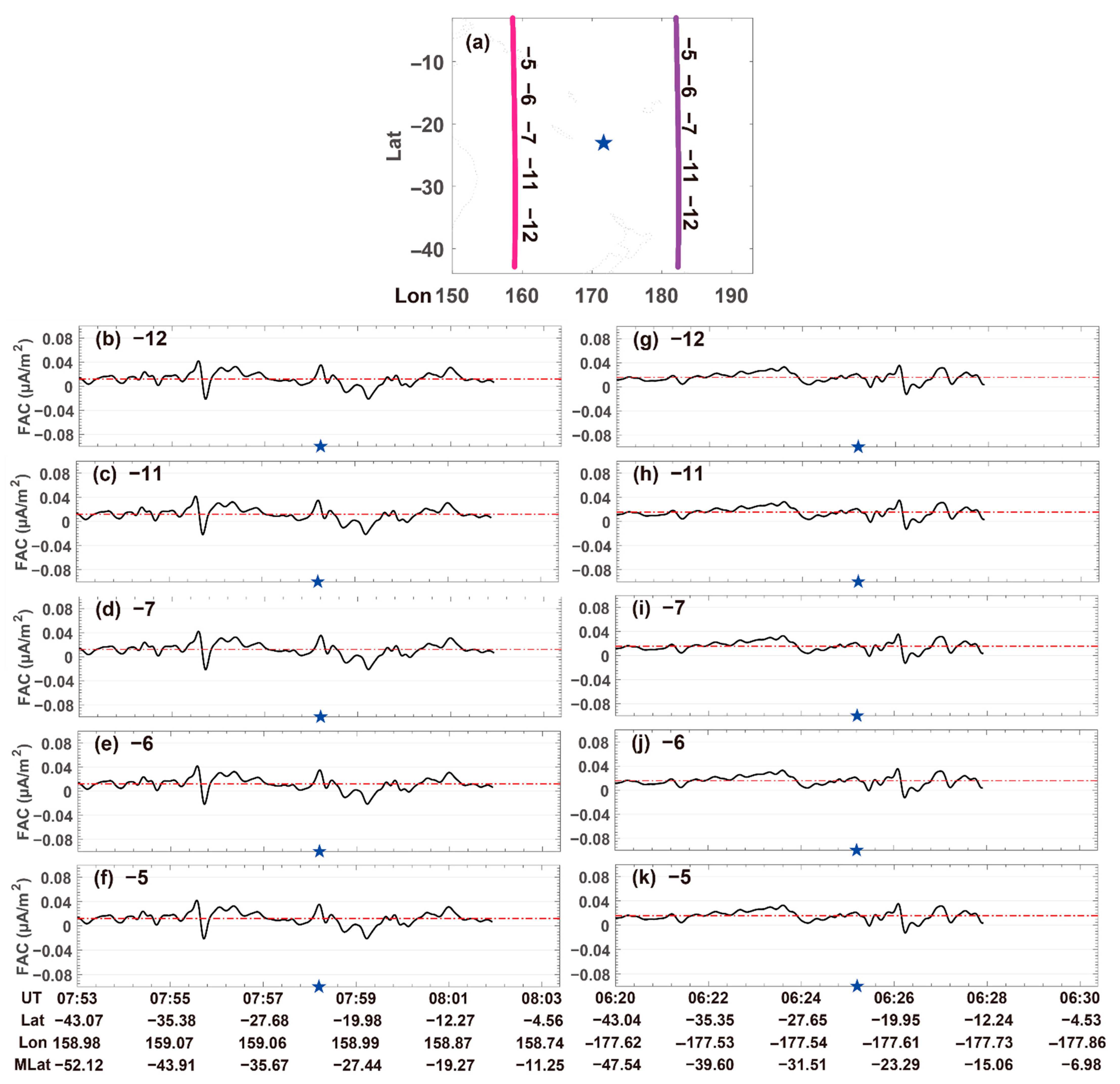
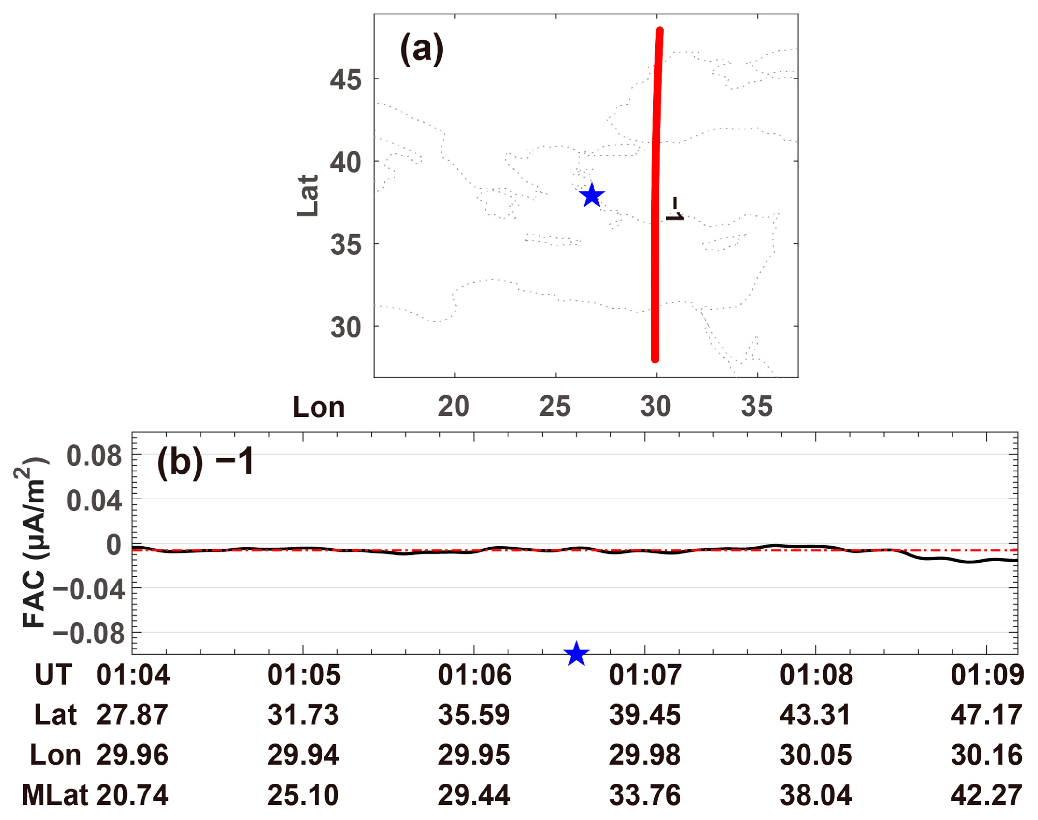
3.3. Relationship with Field-Aligned Currents (FACs)
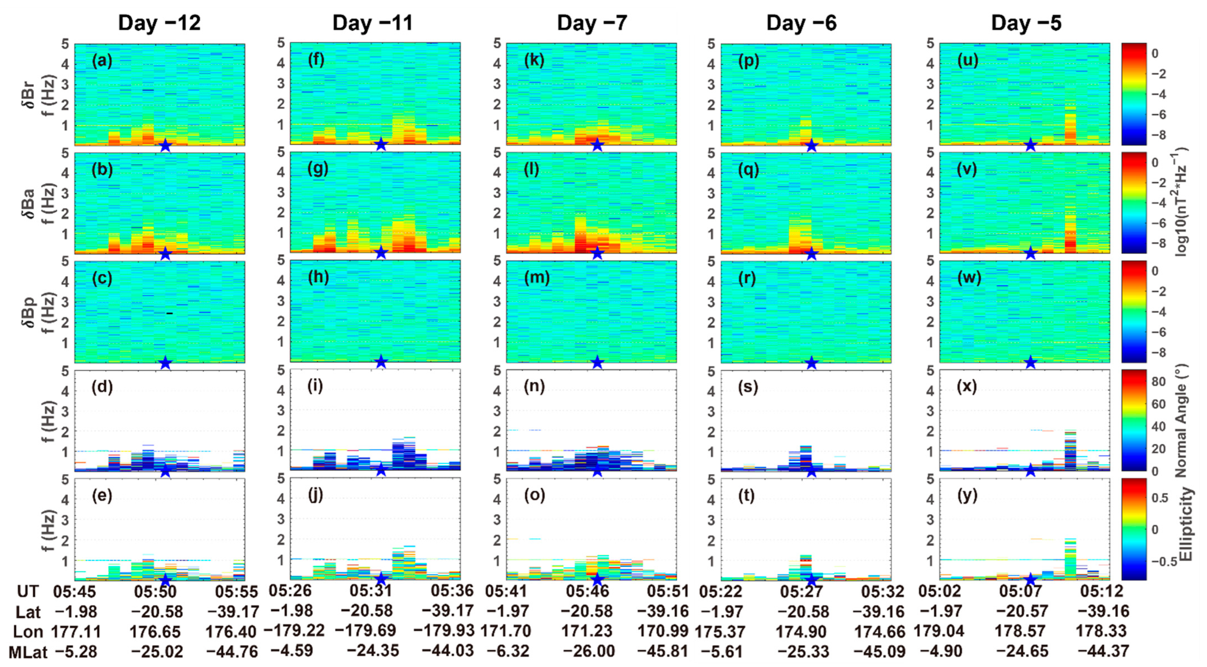
3.4. Analysis of Polarization Parameters
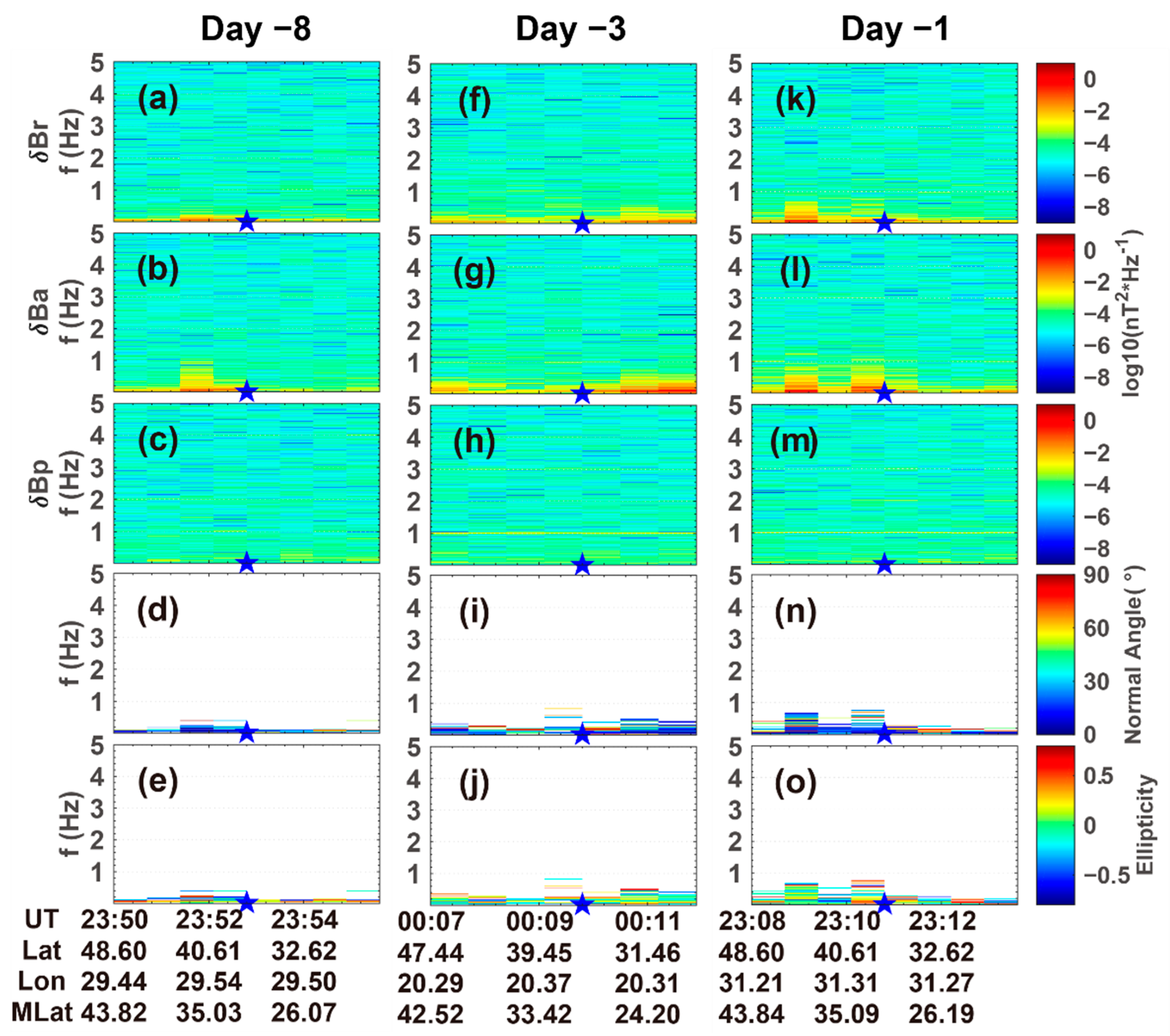
3.5. An Intraplate Earthquake Case Study
4. Discussion
5. Conclusions
Author Contributions
Funding
Data Availability Statement
Acknowledgments
Conflicts of Interest
Appendix A


References
- Zhao, S.; Shen, X.; Liao, L.; Zhima, Z.; Zhou, C.; Wang, Z.; Cui, J.; Lu, H. Investigation of Precursors in VLF Subionospheric Signals Related to Strong Earthquakes (M > 7) in Western China and Possible Explanations. Remote Sens. 2020, 12, 3563. [Google Scholar] [CrossRef]
- Zhang, X.; Wang, Y.; Boudjada, M.Y.; Liu, J.; Magnes, W.; Zhou, Y.; Du, X. Multi-Experiment Observations of Ionospheric Disturbances as Precursory Effects of the Indonesian Ms6.9 Earthquake on 5 August 2018. Remote Sens. 2020, 12, 4050. [Google Scholar] [CrossRef]
- Yumoto, K.; Ikemoto, S.; Cardinal, M.G.; Hayakawa, M.; Hattori, K.; Liu, J.Y.; Saroso, S.; Ruhimat, M.; Husni, M.; Widarto, D.; et al. A new ULF wave analysis for Seismo-Electromagnetics using CPMN/MAGDAS data. Phys. Chem. Earth Parts A B C 2009, 34, 360–366. [Google Scholar] [CrossRef]
- Fraser-Smith, A.C.; Bernardi, A.; McGill, P.R.; Ladd, M.E.; Helliwell, R.A.; Villard, O.G. Low-frequency magnetic field measurements near the epicenter of the Ms 7.1 Loma Prieta earthquake. Geophys. Res. Lett. 1990, 17, 1465–1468. [Google Scholar] [CrossRef]
- Hayakawa, M.; Kawate, R.; Molchanov, O.A.; Yumoto, K. Results of ultra-low-frequency magnetic field measurements during the Guam Earthquake of 8 August 1993. Geophys. Res. Lett. 1996, 23, 241–244. [Google Scholar] [CrossRef]
- Bortnik, J.; Cutler, J.W.; Dunson, C.; Bleier, T.E. The possible statistical relation of Pc1 pulsations to Earthquake occurrence at low latitudes. Ann. Geophys. 2008, 26, 2825–2836. [Google Scholar] [CrossRef] [Green Version]
- Han, P.; Hattori, K.; Hirokawa, M.; Zhuang, J.; Chen, C.-H.; Febriani, F.; Yamaguchi, H.; Yoshino, C.; Liu, J.-Y.; Yoshida, S. Statistical analysis of ULF seismomagnetic phenomena at Kakioka, Japan, during 2001–2010. J. Geophys. Res. Space Phys. 2014, 119, 4998–5011. [Google Scholar] [CrossRef]
- Hattori, K.; Han, P.; Yoshino, C.; Febriani, F.; Yamaguchi, H.; Chen, C.-H. Investigation of ULF Seismo-Magnetic Phenomena in Kanto, Japan During 2000–2010: Case Studies and Statistical Studies. Surv. Geophys. 2013, 34, 293–316. [Google Scholar] [CrossRef]
- Molchanov, O.; Hayakawa, M.; Rafalsky, V. Penetration characteristics of electromagnetic emissions from an underground seismic source into the atmosphere, ionosphere, and magnetosphere. J. Geophys. Res. Space Phys. 1995, 100, 1691–1712. [Google Scholar] [CrossRef]
- Athanasiou, M.A.; Anagnostopoulos, G.C.; Iliopoulos, A.C.; Pavlos, G.P.; David, C.N. Enhanced ULF radiation observed by DEMETER two months around the strong 2010 Haiti earthquake. Nat. Hazards Earth Syst. Sci. 2011, 11, 1091–1098. [Google Scholar] [CrossRef]
- Walker, S.N.; Kadirkamanathan, V.; Pokhotelov, O.A. Changes in the ultra-low frequency wave field during the precursor phase to the Sichuan earthquake: DEMETER observations. Ann. Geophys. 2013, 31, 1597–1603. [Google Scholar] [CrossRef] [Green Version]
- Zhang, X.; Chen, H.; Liu, J.; Shen, X.; Miao, Y.; Du, X.; Qian, J. Ground-based and satellite DC-ULF electric field anomalies around Wenchuan M8.0 earthquake. Adv. Space Res. 2012, 50, 85–95. [Google Scholar] [CrossRef]
- De Santis, A.; Balasis, G.; Pavón-Carrasco, F.J.; Cianchini, G.; Mandea, M. Potential earthquake precursory pattern from space: The 2015 Nepal event as seen by magnetic Swarm satellites. Earth Planet. Sci. Lett. 2017, 461, 119–126. [Google Scholar] [CrossRef] [Green Version]
- Ouyang, X.Y.; Parrot, M.; Bortnik, J. ULF Wave Activity Observed in the Nighttime Ionosphere Above and Some Hours Before Strong Earthquakes. J. Geophys. Res. Space Phys. 2020, 125, e2020JA028396. [Google Scholar] [CrossRef]
- Berthelier, J.J.; Godefroy, M.; Leblanc, F.; Malingre, M.; Menvielle, M.; Lagoutte, D.; Brochot, J.Y.; Colin, F.; Elie, F.; Legendre, C. ICE, the electric field experiment on DEMETER. Planet. Space Sci. 2006, 54, 456–471. [Google Scholar] [CrossRef]
- Savitzky, A.; Golay, M.J.E. Smoothing and Differentiation of Data by Simplified Least Squares Procedures. Anal. Chem. 1964, 36, 1627–1639. [Google Scholar] [CrossRef]
- Kim, H.; Hwang, J.; Park, J.; Miyashita, Y.; Shiokawa, K.; Mann, I.R.; Raita, T.; Lee, J. Large-Scale Ducting of Pc1 Pulsations Observed by Swarm Satellites and Multiple Ground Networks. Geophys. Res. Lett. 2018, 45, 12–703. [Google Scholar] [CrossRef] [Green Version]
- Means, J.D. Use of the three-dimensional covariance matrix in analyzing the polarization properties of plane waves. J. Geophys. Res. 1972, 77, 5551–5559. [Google Scholar] [CrossRef]
- Bortnik, J.; Cutler, J.W.; Dunson, C.; Bleier, T.E. An automatic wave detection algorithm applied to Pc1 pulsations. J. Geophys. Res. Space Phys. 2007, 112, A04204. [Google Scholar] [CrossRef] [Green Version]
- Dobrovolsky, I.P.; Zubkov, S.I.; Miachkin, V.I. Estimation of the size of earthquake preparation zones. Pure Appl. Geophys. 1979, 117, 1025–1044. [Google Scholar] [CrossRef]
- Lühr, H.; Kervalishvili, G.; Michaelis, I.; Rauberg, J.; Ritter, P.; Park, J.; Merayo, J.M.G.; Brauer, P. The interhemispheric and F region dynamo currents revisited with the Swarm constellation. Geophys. Res. Lett. 2015, 42, 3069–3075. [Google Scholar] [CrossRef] [Green Version]
- Ritter, P.; Lühr, H.; Rauberg, J. Determining field-aligned currents with the Swarm constellation mission. Earth Planets Space 2013, 65, 9. [Google Scholar] [CrossRef] [Green Version]
- Stolle, C.; Lühr, H.; Rother, M.; Balasis, G. Magnetic signatures of equatorial spread F as observed by the CHAMP satellite. J. Geophys. Res. Space Phys. 2006, 111, A02304. [Google Scholar] [CrossRef]
- Rodríguez-Zuluaga, J.; Stolle, C.; Park, J. On the direction of the Poynting flux associated with equatorial plasma depletions as derived from Swarm. Geophys. Res. Lett. 2017, 44, 5884–5891. [Google Scholar] [CrossRef] [Green Version]
- Rodríguez-Zuluaga, J.; Stolle, C.; Yamazaki, Y.; Lühr, H.; Park, J.; Scherliess, L.; Chau, J.L. On the Balance Between Plasma and Magnetic Pressure Across Equatorial Plasma Depletions. J. Geophys. Res. Space Phys. 2019, 124, 5936–5944. [Google Scholar] [CrossRef] [Green Version]
- Yokoyama, T.; Stolle, C. Low and Midlatitude Ionospheric Plasma Density Irregularities and Their Effects on Geomagnetic Field. Space Sci Rev. 2017, 206, 495–519. [Google Scholar] [CrossRef]
- Park, J.; Lühr, H.; Stolle, C.; Rother, M.; Min, K.W.; Chung, J.-K.; Kim, Y.H.; Michaelis, I.; Noja, M. Magnetic signatures of medium-scale traveling ionospheric disturbances as observed by CHAMP. J. Geophys. Res. Space Phys. 2009, 114, A03307. [Google Scholar] [CrossRef] [Green Version]
- Yin, F.; Lühr, H.; Park, J.; Wang, L. Comprehensive Analysis of the Magnetic Signatures of Small-Scale Traveling Ionospheric Disturbances, as Observed by Swarm. J. Geophys. Res. Space Phys. 2019, 124, 10794–10815. [Google Scholar] [CrossRef]


Publisher’s Note: MDPI stays neutral with regard to jurisdictional claims in published maps and institutional affiliations. |
© 2022 by the authors. Licensee MDPI, Basel, Switzerland. This article is an open access article distributed under the terms and conditions of the Creative Commons Attribution (CC BY) license (https://creativecommons.org/licenses/by/4.0/).
Share and Cite
Ouyang, X.-Y.; Wang, Y.-F.; Zhang, X.-M.; Wang, Y.-L.; Wu, Y.-Y. A New Analysis Method for Magnetic Disturbances Possibly Related to Earthquakes Observed by Satellites. Remote Sens. 2022, 14, 2709. https://doi.org/10.3390/rs14112709
Ouyang X-Y, Wang Y-F, Zhang X-M, Wang Y-L, Wu Y-Y. A New Analysis Method for Magnetic Disturbances Possibly Related to Earthquakes Observed by Satellites. Remote Sensing. 2022; 14(11):2709. https://doi.org/10.3390/rs14112709
Chicago/Turabian StyleOuyang, Xin-Yan, Yong-Fu Wang, Xue-Min Zhang, Ya-Lu Wang, and Ying-Yan Wu. 2022. "A New Analysis Method for Magnetic Disturbances Possibly Related to Earthquakes Observed by Satellites" Remote Sensing 14, no. 11: 2709. https://doi.org/10.3390/rs14112709
APA StyleOuyang, X.-Y., Wang, Y.-F., Zhang, X.-M., Wang, Y.-L., & Wu, Y.-Y. (2022). A New Analysis Method for Magnetic Disturbances Possibly Related to Earthquakes Observed by Satellites. Remote Sensing, 14(11), 2709. https://doi.org/10.3390/rs14112709