Article

Hyperspectral Image Classification with a Multiscale Fusion-Evolution Graph Convolutional Network Based on a Feature-Spatial Attention Mechanism

1
Zhejiang Provincial Key Laboratory of Geographic Information Science, Hangzhou 310028, China
2
School of Earth Sciences, Zhejiang University, Hangzhou 310027, China
3
Ocean Academy, Zhejiang University, 1 Zheda Road, Zhoushan 316021, China
*
Author to whom correspondence should be addressed.
Remote Sens. 2022, 14(11), 2653; https://doi.org/10.3390/rs14112653
Submission received: 13 April 2022 / Revised: 27 May 2022 / Accepted: 30 May 2022 / Published: 1 June 2022
(This article belongs to the Special Issue Deep Learning for Very-High Resolution Land-Cover Mapping)

Abstract

:
Convolutional neural network (CNN) has achieved excellent performance in the classification of hyperspectral images (HSI) due to its ability to extract spectral and spatial feature information. However, the conventional CNN model does not perform well in regions with irregular geometric appearances. The recently proposed graph convolutional network (GCN) has been successfully applied to the analysis of non-Euclidean data and is suitable for irregular image regions. However, conventional GCN has problems such as very high computational cost on HSI data and cannot make full use of information in the image spatial domain. To this end, this paper proposes a multi-scale fusion-evolution graph convolutional network based on the feature-spatial attention mechanism (MFEGCN-FSAM). Our model enables the graph to be automatically evolved during the graph convolution process to produce more accurate embedding features. We have established multiple local and global input graphs to utilize the multiscale spectral and spatial information of the image. In addition, this paper designs a feature-spatial attention module to extract important features and structural information from the graph. The experimental results on four typical datasets show that the MFEGCN-FSAM proposed in this paper has better performance than most existing HSI classification methods.

1. Introduction

With the rapid development of hyperspectral imaging technology, people can easily obtain hyperspectral images (HSI) containing hundreds of bands of useful information [1]. Nowadays, hyperspectral imaging technology plays an important role in the military, economics, agriculture, environmental monitoring and other fields. The essence of the application of HSI is to classify them. How to quickly and accurately classify each pixel in HSI is the core issue.
People have done a lot of exploration and adopted many methods on the land cover classification based on HSI. The early-staged methods are mainly based on conventional pattern recognition methods, such as nearest neighbor classifier and linear classifier, including the classic k-nearest-neighbor algorithm [2] and support vector machine (SVM) [3]. Besides, there are many methods that have been further used to improve the performance of HSI classification, such as extreme learning machines [4], and sparse representation-based classifiers [5].
However, it is difficult to accurately distinguish features using only spectral information [6]. Many researchers used the spatial texture features of the image to design classifiers for spectral and spatial information and achieved better classification results [7,8]. Spectrum-spatial classification methods can generally be divided into two categories. The first method extracts spatial feature information and then combines it with spectral features [9,10]. The second method directly combines spatial information with spectral features and uses joint features to classify [11]. In addition, some scholars divided HSI into superpixels based on the spectral and spatial data of HSI and input the feature data of superpixels into SVM to obtain the classification results of HSI [12,13,14]. Recently, some scholars have proposed a superpixel-based HSI classification method using sparse representation [15,16] and achieved good classification results.
Many conventional feature extraction methods are based on hand-made features and heavily depend on professional knowledge and experience. In recent years, deep learning methods have received widespread attention due to their powerful representation ability and have been widely used in HSI classification tasks [17,18,19,20,21]. The deep learning method does not rely on artificially designed shallow features. It can automatically acquire the high-level features of the features by gradually aggregating the low-level features in the data. These features have achieved great success in machine vision tasks. Chen et al. [17] first used deep learning methods for HSI classification. They used stacked autoencoders (SAE) and deep belief networks (DBN) for feature extraction and classification in spectral space. Subsequently, a convolutional neural network (CNN) was widely used in HSI classification due to its powerful image processing capabilities [22,23,24]. Hu et al. [25] proposed 1-D CNN to directly classify HSI in the spectral domain. Chen et al. [26] proposed 3-D CNN to extract the spectral and spatial features of HSI at the same time and achieved good results. Haque et al. [27] proposed a lightweight 3D–2D convolutional neural network framework, which reduces the computational burden through data dimensionality reduction, and uses 3D and 2D convolution operations to extract spatial and spectral features, obtaining good results and achieving high classification accuracy.
However, CNN models only convolve on regular square regions, so they cannot adaptively capture the geometric changes of different object regions in HSI. In addition, when convolving all image blocks, the weight of each convolution kernel is the same. This leads to the CNN possibly losing information regarding the class boundary in the process of feature abstraction, and misclassification may occur due to the fixed convolution kernel. In other words, the convolution kernel with a fixed shape, size, and weight are not suitable for all regions in the HSI. In addition, due to the existence of a large number of parameters, CNN-based methods usually require a long training time.
In addition to CNN, some other categories of networks are also used to classify HSI. As a widely used model in the field of image segmentation, a fully convolutional network (FCN) [28] has been successfully applied to the HSI classification task. The model uses convolutional layers and pooling layers, which can effectively learn the deep features of HSI and improve the classification performance. Furthermore, as a feedforward neural network, recurrent neural networks (RNN) [20] have been studied for HSI classification tasks. RNN can build a sequential model to effectively simulate the relationship between adjacent spectral bands. In the meantime, generative adversarial network (GAN)-based [29] has also been introduced for HSI classification. In recent years, Sun et al. [30] introduced the Transformer framework to the HSI classification task, and they used a spectral-spatial feature tokenization transformer (SSFTT) method to capture both spectral-spatial features and high-level semantic features and achieved good results.
Compared with the method mentioned above, graph convolutional networks (GCN) [31] can be directly applied to non-Euclidean data. In [32,33], GCN was applied to HSI classification. However, some problems will occur when the conventional GCN is directly applied to HSI classification. First, due to noise pollution in HSI, the edge weights of paired pixels may not represent their inherent similarity, which may lead to inaccuracy in the initial construction of the input image. In addition, GCN can only use the spectral features of the image but ignore the spatial features and the computational cost of directly using pixels as nodes to construct a graph is unbearable. In response to these problems, Wan et al. [34] proposed a multiscale dynamic graph convolutional network (MDGCN) and achieved good results. However, there are some problems with MDGCN. For example, a multiscale fusion of spectral and spatial embedded information is directly spliced and added, and there are no multiple weights to correspond to different scales of information. The model treats all neighboring nodes equally when constructing the graph and cannot assign different weights to nodes based on their importance. Only the neighborhood information is considered, and the global spatial information of remote sensing images is ignored.
Based on the aforementioned background, we present a method called ‘multiscale fusion-evolution graph convolutional network based on feature-spatial attention mechanism’ (MFEGCN-FSAM). We refer to the method of [34], using a superpixel segmentation algorithm to segment the image into a certain number of superpixels and regard each superpixel as a node in the graph. Through this method, the computational cost on the graph will be greatly reduced, and the impact of over-fitting can be reduced at the same time. In order to make full use of the multiscale spatial and spectral context information of HSI, this paper establishes input graphs locally and globally at different scales to flexibly capture spatial and spectral features at different scales. This paper proposes a fusion evolution method by which the graph can be automatically evolved to make the feature embeddings more accurate during the convolution process. The model introduces the attention mechanism, which assigns corresponding weights to the nodes in the graph and has achieved good results in experiments.
To sum up, the main contributions of the proposed MFEGCN-FSAM are as follows:
First, we propose a fusion evolution method that enables the graph to be continuously updated during the convolution process to generate feature embeddings more accurately. Instead of using the initial fixed graph for convolution, we designed a fusion and evolution method. In the process of graph convolution, the structural information and node embeddings of the current graph are fused, and the graph structure evolves and updates accordingly. Therefore, this method can make the graph continuously updated during the convolution process to generate more accurate feature embeddings. The operations of graph fusion and evolution are constantly alternated during the training process, which works collaboratively to produce more reasonable graph structures and promising classification results.
Second, we establish input graphs locally and globally at different scales. In order to take the multiscale information into consideration, we construct input graphs locally and globally at different scales to fully utilize the spatial and spectral information of HSI. Unlike the common GCN models that only use one fixed graph, the multiscale design enables MFEGCN-FSAM to extract spectral-spatial features with different receptive fields so that comprehensive contextual information from different levels can be integrated.
Third, we design a feature-spatial attention module, which effectively highlights the important information in the graph by paying attention to the important local structures and features of the graph to enhance the representation ability of the model.
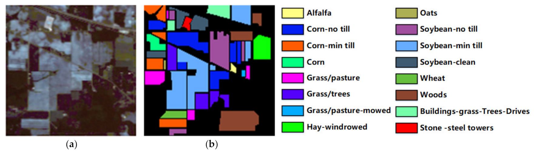
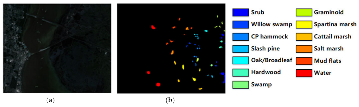
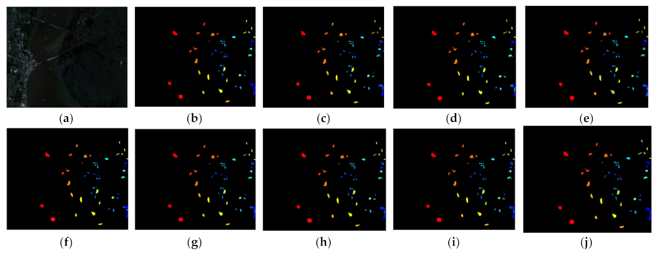
Finally, experimental results on four typical hyperspectral image datasets show that MFEGCN-FSAM achieves good performance compared to existing methods.
The remainder of this paper is organized as follows. Section 2 first provides an introduction to the relevant background. Section 3 introduces the MFEGCN-FSAM method we proposed in detail. Section 4 is the experimental results and analysis. Finally, we summarize the work and conclude this paper in Section 5.

2. Related Works

2.1. Graph Convolutional Network

Many scientific fields study data with an underlying structure that is non-Euclidean, such as social networks in computational social sciences, sensor networks in communications, functional networks in brain imaging and regulatory networks in genetics. In many applications, such geometric data are large and complex (in the case of social networks, on the scale of billions) and are natural targets for machine-learning techniques [35]. The graph is an important type of non-European data. Many conventional deep learning methods are often applied to Euclidean data but cannot be applied to feature extraction and application of graph data. Therefore, some scholars have carried out exploration and research on this demand.
Gori et al. [36] first proposed the concept of the neural network method applied to graph data. Compared with RNN and CNN, the advantage of this method is that it can operate on non-Euclidean data with graph structure. Specifically, the graph neural network (GNN) can gather the features of the nodes on the graph and correctly embed the entire graph into the new distinguishing space. Subsequently, Scarselli et al. [37] used a supervised learning algorithm to make it easier for GNN to train on actual data.
However, their algorithm is computationally expensive and time-consuming on large-scale graph data. Therefore, Bruna et al. [38] developed a graph convolution operation based on spectral characteristics, which convolves on the neighborhood of each graph node and produces node-level output results. After that, many expansion methods of graph convolution were derived and achieved good results. For example, Hamilton et al. [39] proposed a ‘GraphSAGE’ based on an inductive framework that can use node features to generate node embeddings for previously invisible data. In addition, Defferrard et al. [40] put forward the expression of CNN in the context of spectrogram theory. Based on previous work, Kipf et al. [31] proposed a GCN model that can simultaneously encode graph structure and node features to quickly approximate local convolution, simplifying GCN through the first-order approximation of graph convolution, which makes the filtering operation is more effective. With the rapid development of graph convolution theory, GCN is widely used in different fields, such as recommendation systems [41] and semantic segmentation [42].
In summary, GCN runs on a graph, which can aggregate and transform the feature information of the neighbors of each graph node. Therefore, the convolution operation of GCN is adaptively controlled by the domain structure of the graph, so GCN can be based on a predefined graph Applied to non-Euclidean irregular data. In addition, node features and local graph structures can be coded through learned hidden layers, so GCN can exhaustively utilize image features and flexibly retain class boundaries. At present, some scholars have applied GCN to HSI classification [32].

2.2. Hyperspectral Image Classification

There are many methods used in the field of HSI classification, such as random forest [43] and SVM [44]. SVM shows good classification performance for a data set with a limited number of labeled samples [45], but it cannot utilize the spatial information of the image. In order to solve this problem, Camps-Valls et al. [46] designed a composite score that can use spatial information. In addition, the Markov random field (MRF) method [47] utilizes the spatial context information of HSI, assuming that adjacent pixels may be of the same category.
However, the above methods are to manually extract the spectral and spatial features of HSI, which are empirical. The methods based on deep learning [48] can automatically learn features from HSI data, which are more and more widely used in HSI classification tasks. Chen et al. [17] first introduced a SAE for HSI classification to learn hierarchical features in an unsupervised manner. Subsequently, Chen et al. [1] utilized DBN to obtain the robust features from HSI. Meanwhile, Shi and Pun [49] introduced RNN into the HSI classification task and utilized RNN to obtain multiscale spectral, spatial features, which can learn the spatial dependence of non-adjacent image patches in the two-dimensional space domain. Furthermore, Zhu et al. [29] applied GAN to HSI classification with three PCA components and random noise as input. Sun et al. [30] used 2D and 3D convolution modules to extract shallow spectral and spatial features and used a Gaussian weighted feature tokenizer for feature transformation, and finally inputted the transformed features into the Transformer encoder module for feature representation and learning. Among these deep learning methods, CNN, due to its weight-sharing characteristics, requires fewer parameters than a fully connected network with the same number of hidden layers, so it has attracted much attention in the application of large-scale HSI data.
According to the input information of the model, CNN-based HSI classification methods can be divided into three categories: spectral CNN, spatial CNN, and spectral-spatial CNN. Spectral CNN-based HSI classification methods take each pixel vector as the input of the model and utilize the CNN model to classify HSI directly in the spectral domain. Hu et al. [25] proposed a 1D-CNN model to extract the spectral features of pixels to classify HSI. Mining spatial information is very important in HSI classification; spatial CNN-based methods usually use 2D CNN to extract spatial features of HSI. Makantasis et al. [23] proposed 2D-CNN to extract the spatial features of HSI. Spectral-spatial CNN-based methods aim to exploit joint spectral-spatial HSI features in a unified framework. Yang et al. [50] proposed a 1D + 2D CNN framework for HSI classification, which can separately extract spectral and spatial features of HSI and connect them to obtain the joint spectral and spatial features. Chen et al. [26] proposed 3D-CNN to extract the joint spectral, spatial features of HSI, which combined with regularization technology to make the model more generalized. Although the CNN-based method shows superior performance in HSI classification, due to its fixed convolution kernel design, it cannot handle the geometric changes of image regions well, and its performance in class boundary classification is limited.
Since GCN can be calculated on non-European data with a graph structure, it can flexibly retain class boundary information; GCN has been applied to HSI classification [32]. The main idea of the GCN-based HSI classification method is to treat each pixel of the HSI as a node to construct a graph and to predict the category of each node in the graph, which is more flexible than the square fixed convolution kernel used by CNN. For example, Mou et al. [33] took the entire image, including labeled and unlabeled pixels, as input and utilized a set of graph convolutional layers to extract features. However, GCN uses each pixel of HSI as a node to construct the graph, which makes the calculation and storage cost of the adjacency matrix very huge, which limits the application of GCN in HSI classification. Wan et al. [34] performed superpixel segmentation on HSI, using superpixels as nodes of the graph. In addition, Hong et al. [51] reduced the calculation of the adjacency matrix by randomly extracting nodes in the HSI to construct a subgraph and used mini-batch training to speed up gradient descent. However, the way of randomly extracting nodes to construct subgraphs in HSI obviously breaks the original spatial adjacency relationship of ground objects in HSI, which makes the model performance obviously limited. In addition, these works cannot make full use of the information of different scales, from global to local. Each node in the graph does not have different weights, and the current embedding and graph structure cannot be well integrated to update the graph. In this article, we propose MFEGCN-FSAM to provide a solution to the above problems.

3. Method

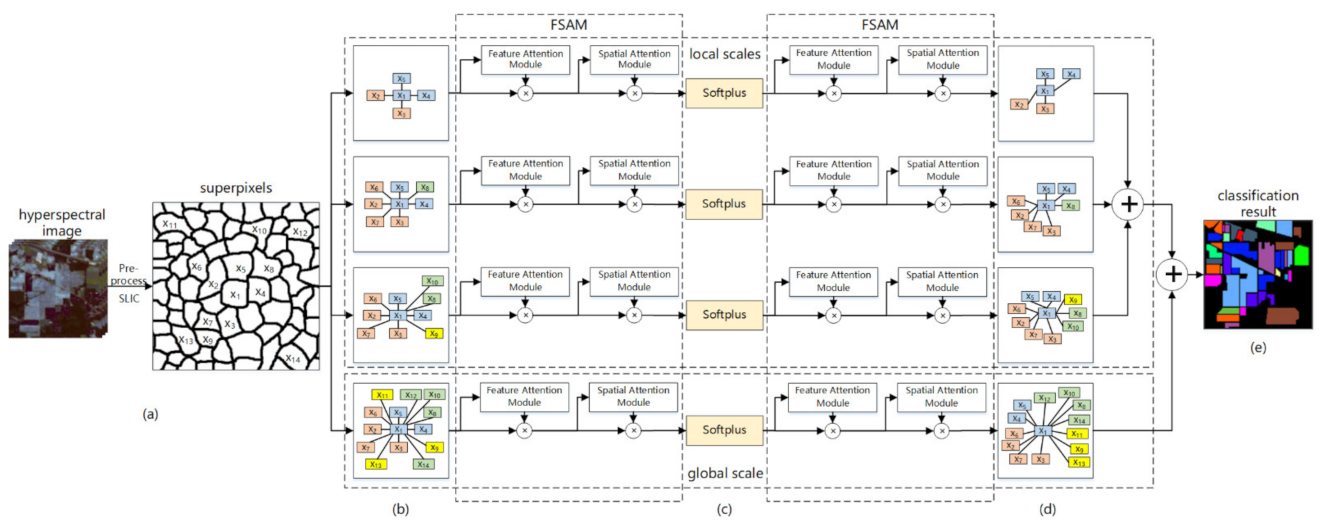
This section details the MFEGCN-FSAM model we proposed (see Figure 1). There are four different spatial scales in our model, and each scale has two convolutional graphs layers. When the HSI data is given, a series of preprocessing, such as denoising and normalization, are first performed. Then, the image will be segmented into several superpixels by the simple linear iterative clustering method (SLIC) [42]. The superpixels are used as nodes in different spatial scales to participate in the construction of multiscale graphs. Input the constructed graph into the feature-spatial attention module (FSAM), and the input graph is processed by the FSAM to obtain the output graph features corrected by the feature and spatial attention. The graph convolution operation is performed on these graphs to aggregate the spectral-spatial feature information, our proposed fusion evolution method can make the model fuse the structural information and data embeddings of the current graph during the convolution process, and the graph structure evolves and updates accordingly. Finally, the global and local classification results will be generated by the classifier, and the final result is obtained by adding the trainable weight parameters.

3.1. Graph Convolutional Network Framework

GCN [36] is a neural network that runs directly on the graph and gradually fuses features in the neighborhood to generate node embeddings. An undirected graph can be defined as G = V , E , where V is the set of nodes and E are edges. Here A is defined as the adjacency matrix of G . By referring to the radial basis function (RBF), the calculation formula of A is defined as follows:
A i j = e x i x j 2 σ 2 ,           i f     x j N x i   o r   x i N x j 0 ,                                               o t h e r w i s e
where σ is the width parameter of the function, which controls the radial range of the function, x i   represents a node and N x i is the set of neighbors of x i .
The Laplacian matrix of G is defined as L = D A , and D is the degree matrix of A . The core of GCN is based on the spectral decomposition of the Laplacian matrix L . The spectral decomposition of L is:
L = U λ 1 λ n U 1
where U = u 1 , u 2 , , u n , is a matrix with column vector as unit eigenvector, u i is the column vector, λ 1 λ n is a diagonal matrix composed of n eigenvalues. Since U is an orthogonal matrix, so the above formula can be written as
L = U λ 1 λ n U T
According to the Convolution Theorem, the Fourier transform of the convolution integral of two functions f t and h t is equal to the product of the transforms of the functions. The convolution formula of f and h is as follows:
f h = F 1 f ̂ ω h ̂ ω = 1 2 Π f ̂ ω h ̂ ω e i ω t d ω  
According to Inverse Fourier transform, f = U f ̂ , h = U h ̂ , thus f h = U U T f U T h . The convolution kernel h can be written in the form of a diagonal matrix diag h ̂ λ l according to the following formula:
f h = h f = h 1 h n f 1 f n = h 1 0 0 h n f 1 f n
Therefore, the formula of graph convolution is:
f h = U h ̂ λ 1 h ̂ λ n U T f
Bruna [38] et al. optimized the convolution kernel, diag h ̂ λ l is changed to diag θ l , that is g θ = diag θ l . Then the output of the convolution is:
y output   = g θ x = U g θ U T x
However, this method has drawbacks. Firstly, U g θ U T will be calculated for each forward propagation, which is too expensive. Secondly, the convolution kernel does not have local properties, the matrix calculated by the convolution kernel has non-zero elements in all positions, which means that this is a global, fully connected convolution kernel.
Defferrard et al. [40] proposed a method without decomposing the Laplacian matrix, which is the Chebyshev polynomial approximation method:
g θ Λ k = 0 K 1 θ k T k Λ ̃
where the parameter θ is a vector of Chebyshev coefficients, Λ is a diagonal matrix containing the eigenvalues of Laplacian Matrix L , T k Λ ̃ is the Chebyshev polynomial of order k evaluated at Λ ̃ = 2 λ max Λ I N , λ max is the largest eigenvalues of L .
Substituting Formula (8) into Formula (7), y output = U k = 0 K 1 θ k T k Λ ̃ U T x . According to the properties of Chebyshev polynomials, y output   can be written as, y output = k = 0 K 1 θ k T k U Λ ̃ U T x that is:
y output = k = 0 K 1 θ k T k L ˜ x
where L ˜ = 2 λ max L I N , and it is easy to notice that U Λ U k = U Λ k U . Now the value of convolution depends on the Kth-order neighborhood of the central node. Kipf et al. [31] assumed that λ max 2 and limited K = 1 , thus the Formula (10) is transformed into the following form:
y output   = g θ x θ 0 x + θ 1 L I N x = θ 0 x + θ 1 D 1 2 A D 1 2 x
Then assume that the parameters θ 0   and θ 1 are shared in the entire figure, the Formula (10) becomes as follows:
y output   = g θ x θ I N + D 1 2 A D 1 2 x
At this point, the formula has become very concise, but there is still a problem. The value range of the eigenvalue of I N + D 1 2 A D 1 2 is [0, 2]. Repeated calculation of this formula in the network will cause numerical instability and gradient explosion or disappearance. To solve this problem, Kipf et al. [31] used the renormalization to change I N + D 1 2 A D 1 2 to D ̃ 1 2 A ̃ D ̃ 1 2 , where A ̃ = A + I N , D ̃ i i = j A ̃ i j , the Formula (11) is as follows:
Z = D ̃ 1 2 A ̃ D ̃ 1 2 X Θ
where   Z is the result of convolution output, X is the input node feature matrix, Θ is the convolution parameter matrix. To apply the Formula to GCN, we can define that:
H l + 1 = σ A ^ H l W l
where A ^ = D ̃ 1 2 A ̃ D ̃ 1 2 , H l   is the first layer, H 0 = X , W is the weight matrix to be trained, and σ is the activation function. Now, the definition of GCN has been completed.

3.2. Superpixel Segmentation

A HSI often contains tens of thousands or more pixels. If the conventional GCN method is used to construct a graph with each pixel as a node, then the computational consumption is unbearable, and the requirements for computing equipment will be greatly increased. Therefore, in order to solve this problem, this article refers to [34] aggregating the pixels with similar spatial and spectral characteristics in HSI into several superpixels. The average value of the spectra of all pixels in the superpixel in each band is taken as its feature vector. Specifically, the superpixel segmentation algorithm used in this paper is SLIC [42], which is relatively good in terms of the result of generating superpixels and the running speed. However, the SLIC algorithm is designed for RGB images and cannot be used on images with multiple bands. This paper extends the SLIC algorithm so that it can run on HSI. The algorithm details are as follows:
(a)
Initialize the seed point
Suppose we perform superpixel segmentation on an HSI with N pixels, and the preset number of superpixels is k . Let the seed points be evenly distributed in the HSI, the number of pixels contained in each superpixel is N / k , and the distance between each seed point is about S = N / k . Define the feature vector of each seed point as C i = B 1 i , B 2 i , , B n i , X i , Y i T , where B 1 i , B 2 i , , B n i is the spectral vector corresponding to the seed point, X i , Y i is the coordinate value of the seed point, i 1 , k .
(b)
Move the seed point
The seed point is moved to the position with the lowest gradient in its surrounding 3 × 3 neighborhood. This is done to avoid seed points lying on edges and to reduce the chance that the seed points will pick up noisy pixels.
(c)
Assign pixels to the seed point
We define the spectral distance between the pixel point and the seed point as d c = n N ( b j n b i n ) 2 , the spatial distance as d s = ( x j X i ) 2 + ( y j Y i ) 2 , where j is the number of the pixel. The comprehensive distance between the pixel and the seed point as D = d c 2 + ( d s S ) 2 × m 2 where m is the shape parameter, the larger m is, the more regular of superpixels is. Calculate the distance D between the pixels within the 2 S 2 S range of each seed point and the seed point and assign each pixel to the seed point with the smallest distance D from it.
(d)
Update the seed point
Calculate the mean of the feature vector a of all pixels within each superpixel and set it as the new seed point feature vector.
(e)
Iterative calculation and post-processing
Repeat steps c and d until the preset number of iterations is reached, which is set to 10 in this paper. After the segmentation is completed, the connectivity of the superpixels is detected, and the superpixels with a connected component greater than 1 will be separated. If a superpixel contains less than five pixels, assign it to the superpixel that has the most contact with it. We refer to the design of Ren et al. [53] and use CUDA tools to accelerate superpixel segmentation by a factor of nearly 80 with GPU acceleration.

3.3. Graph Fusion Evolution

Although GCN can effectively calculate and aggregate information on graph data, one of its main disadvantages is that the graph constructed by GCN is fixed throughout the process. If the initial input graph is not accurate enough, it will affect the accuracy of the final result of the model. In order to solve this problem, this paper proposes a fusion evolution mechanism on the graph, by fusing the result information of the current convolution output with the previous layer’s graph, and then allowing the graph to be automatically updated during the convolution process.
We define the adjacency matrix of the l layer as A ^ l R n × n and the data embedding H l R n × f output by the first layer, where n is the number of nodes in the graph, and f is the feature dimension of each node. Our goal is to obtain the A ^ l + 1 of next layer. Canonical correlation analysis (CCA) is a method in the field of mathematical statistics to measure the linear relationship between two sets of multidimensional variables [54]. Drawing on the idea of CCA, we propose a feature-level fusion method for graph structure information and embedding information. This fusion method not only helps the model to perform effective feature fusion, but also eliminates redundant information in the data, which is conducive to accurate and efficient update of the graph. We define H ^ = H l ( H l ) T , H ^ R n × n to make the embedding self-aggregate. H ^ is a real symmetric matrix, and the shape is the same as A ^ l , which is conducive to subsequent calculations.
According to the idea of CCA and taking into account the calculation performance, we define a pair of projection vectors V A , V T , project A ^ l and H ^ to obtain A * = V A T A ^ l and H * = V H T H ^ .
Suppose that S A ^ A ^ R n × n and S H ^ H ^ R n × n denote the covariance matrices of A ^ l and H ^ , respectively, while S A ^ H ^ R n × n denotes covariance matrices of A ^ and H ^ . Then the overall covariance matrix S , which contains all the information on associations between pairs of features, can be denoted as:
S = cov A ^ cov A ^ , H ^ cov H ^ , A ^ cov H ^ = S A ^ A ^         S A ^ H ^ S H ^ A ^         S H ^ H ^
Now we hope to find a pair of linear combinations A * = W A T A ^ l and H * = W H T H ^ that maximize the correlation coefficient between A * and H * . We can define the correlation function as follows:
c o r r A * , H * = c o v A * , H * v a r A * v a r H *
According to the definition, the expressions of variance and covariance of A * and H * can be obtained as follows:
c o v A * , H *         = V A T S A ^ H ^ V H v a r A *         = V A T S A ^ A ^ V A v a r H *         = V H T S H ^ H ^ V H
Thus, Formula (16) can be written as:
c o r r A * , H * = V A T S A ^ H ^ V H V A T S A ^ A ^ V A V H T S H ^ H ^ V H
According to the characteristics of Function (19), we can define the constraints of A * and H * :
v a r A * = v a r H * = 1
Now the optimization problem is:
o p t i m i z e m a x i m i z e   c o r r A * , H * v a r A * = v a r H * = 1
Using the Lagrange multiplier method to solve the problem:
L A * , H * = c o v A * , H * λ 1 2 v a r A * 1 λ 2 2 v a r H * 1
where λ 1 and λ 2 are Lagrange multipliers.
By transforming the partial derivative of L , we get:
λ 1 = λ 2 = c o v A * , H * S A ^ A ^ 1 S A ^ H ^ S H ^ H ^ 1 S H ^ A ^ V A = λ 2 V A S H ^ H ^ 1 S H ^ A ^ S A ^ A ^ 1 S A ^ H ^ V H = λ 2 V H d e f i n e   λ = λ 1 = λ 2
The problem is transformed into solving the largest eigenvalue λ and the corresponding eigenvectors V A . Finally, bring the λ and V A into (22) to solve V H :
After solving V A and V H , we can obtain their corresponding projection matrix W A = V A V A T and W H = V H V H T . We can obtain fusion of the current layer between A * and H * by using the summation method, namely:
F l = W A A ^ l + W H H ^
Referring to the design of [55], for the node x l in H l , it is assumed that x l obeys Gaussian distribution with the covariance of A ^ l and the unknown mean μ l , namely p x l = N ( x l | μ l , A ^ l ) . The preliminary fusion result can be defined as:
u l = W A 1 2 x l + W H 1 2 H l
It can be seen that such a fusion method utilizes the structural information and the data embedding of the current graph to improve the graph, making the graph and the data embedding of the next layer more accurate. However, if it is directly input to the next layer, the fusion may cause performance degradation due to the inaccuracy of H l and the lack of structural information in the initial graph.
We must emphasize the structural information of the initially constructed graph. The process of constraining the fusion result F l of the current layer can be considered as a cross-diffusion process between the initial graphs A ^ i n i t and F l . Based on the above definition, we define the expression of the node at the next layer as:
x l + 1 =   A A ^ i n i t u l + η ε
where s is white noise, i.e., p ε = N ( ε | 0 , 1 ) and η is the weight parameter of ε . Under this linear operation, we have:
p ( x l + 1 | u l ) = N ( x l + 1 | A ^ i n i t u l , η 2 I )
According to the total probability formula, we can obtain the distribution of x l + 1 :
p x l + 1 = N ( u l | μ l , F l ) N ( x l + 1 |   A A ^ i n i t u l , η 2 I ) d u l = N ( x l + 1 |   A A ^ i n i t μ l , A ^ i n i t F l   A A ^ i n i t T + η 2 I )
Recalling the previous assumptions, x l + 1 should also obey the Gaussian distribution with the covariance A ^ l + 1 , so that we can obtain A l + 1 as:
A ^ l + 1 = A ^ i n i t W A A ^ l + W H H ^ A ^ i n i t T + η 2 I
In summary, the design of an automatic update graph has three advantages: firstly, the graph is continuously updated during the convolution process, which can make the graph and embedded information more accurate; secondly, the graph is robust to noise and data scale during the update process; thirdly, the graph retains the intrinsic structure of the similar manifold of the entire dataset during the update process.

3.4. Multiscale Contextual Information Integration

Due to the limitation of the convolution kernel, as the number of network layers and iterations of GCN increase, the characteristics of each node will tend to be smooth. In order to solve this problem, Chiang et al. [56] modified the regularization method of the convolution kernel to solve the problem of high power operation of the convolution kernel. Sami [57] et al. abandoned the deep-level convolution features and retained and spliced the results of the multiscale low-level into features. In the classification of HSI, multiscale information has proved to be extremely useful [58] because, in HSI, ground features usually contain different geometrical characteristics. The semantic information obtained from different scales can help people obtain rich local information about the image area.

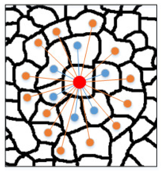
3.4.1. Local Contextual Information

At scale s, each superpixel node xi will be connected to its s-order neighbors. Taking the two-order scale as an example, the 1-order neighbors and second-order neighbors of the central superpixel node xi will be connected to it, as shown in Figure 2.
The neighbors of xi can be expressed as the Formula (28):
R s x i = R s 1 x i R 1 R s 1 x i
where R 0 x i = x i and R 1 x i is the 1-order neighbors set of xi. The neighbors closer to the central node are aggregated more times, which means that the neighbors closer to the central node have a greater impact on the central node.
For the sake of practical significance and efficiency, this paper constructs local graphs as scale 1, 2, and 3. Therefore, the graph convolution layer of scale s can be defined as Formula (29):
H s l + 1 = σ A ^ s H s l W s l
The output of the local-level layers will be added as in Formula (30):
o u t p u t l o c a l = s λ s H s
where λ s is trainable weights corresponding to each layer.

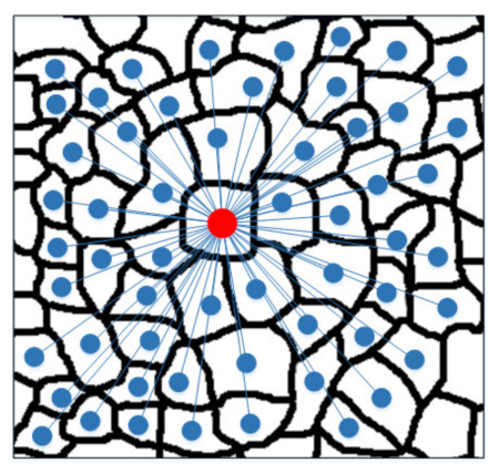
3.4.2. Global Contextual Information

If there are only local graph convolutional layers, the information of the global context in the HSI may not be used, so this paper designs a graph convolutional layer based on the global context. Specifically, we consider that all superpixel nodes in the HSI have an adjacency relationship in pairs and constructed an adjacency matrix as Formula (31).
A g l o b a l = e x i x j 2 σ 2   i f   x i x j
where   x i represents a node and x j another node in the graph, as shown in Figure 3.
However, the dense connection of all superpixel nodes in pairs will cause many problems, such as increased computational cost, and some dissimilar nodes are incorrectly connected together. To solve this problem, this paper sets a threshold β for the global adjacency matrix. The larger the threshold β, the more similar the two nodes are. Only node connections greater than β can be retained. Thus, the above formula becomes Formula (32).
A g l o b a l = e x i x j 2 σ 2 ,   i f   e x i x j 2 σ 2 > β 0 ,                                         o t h e r w i s e
where threshold β is set to 0.8 throughout the experiments.
The global graph convolution layer can be defined as:
H g l o b a l l + 1 = σ A ^ g l o b a l H g l o b a l l W g l o b a l l
The output of the global graph convolution layer is:
o u t p u t g l o a b l = λ g l o b a l H g l o b a l
The final output of the method is:
o u t p u t t o t a l = o u t p u t g l o a b l + o u t p u t l o c a l

3.5. Feature-Spatial Attention Module

Petar et al. [59] mentioned that one of the serious shortcomings of GCN is that GCN treats all neighboring nodes equally and cannot assign different weights to nodes based on their importance. This article refers to the design of CBAM [
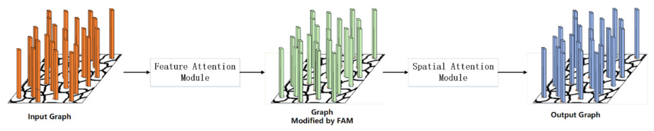
60] and proposes the FSAM (as shown in Figure 4) suitable for GCN, which contains two submodules: a feature attention module and a spatial attention module. In order to emphasize the meaningful information of the two dimensions of the feature axis and the spatial axis, the graph will pass through the feature attention module and spatial attention module sequentially. In this way, the model can learn the “what” and “where” in the feature axis and the spatial axis are important, and the information can flow accurately in the network. In summary, FSAM improves the representational ability of the model by focusing on the important information on the graph and suppressing the other.

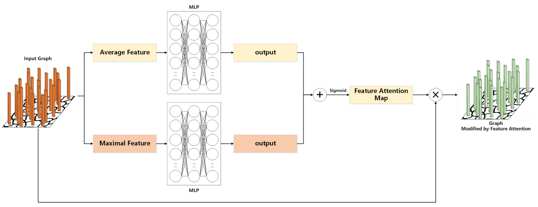
3.5.1. Feature Attention Module

The feature attention module (see Figure 5) tries to find which features of a graph node are important and which should be ignored. In order to aggregate the spatial information of the graph, the module averages and maximizes the graph on the spatial axis. The realization of the module is as follows.
For the input graph G , we first aggregate the spatial information by averaging and maximizing the spatial dimensions of the input graph to generate F a v g and F m a x , which represent the averaged feature and the maximized feature, respectively. F a v g and F m a x will be input into a fully connected network composed of a multi-layer perceptron (MLP), and then the output feature vectors F a v g and F m a x will be obtained. The elements of F a v g and F m a x are summed and combined to obtain the feature attention map M f e a t u r e . The formula for calculating spectral attention is as follows:
M f e a t u r e = σ M L P A v g G + M L P M a x G = σ M L P F a v g + M L P F m a x = σ F a v g + F m a x
where σ is the activation function.

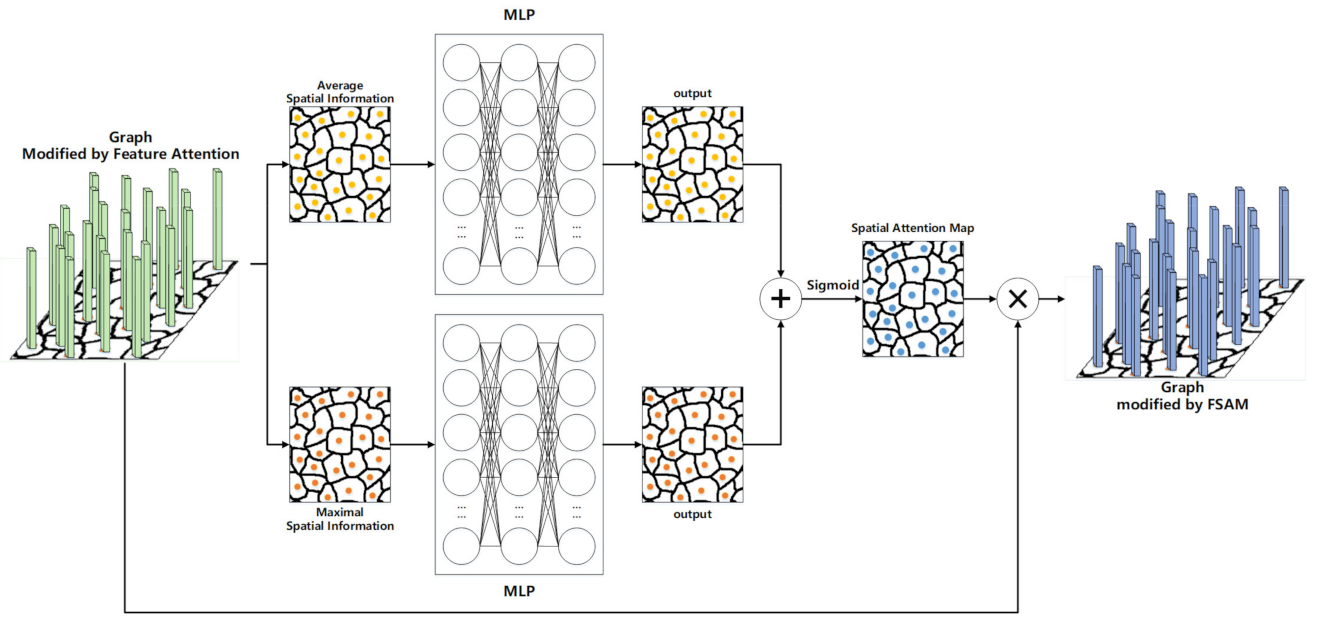
3.5.2. Spatial Attention Module

We generate the spatial attention map by using the spatial relationship between nodes. Unlike the feature attention module, the spatial attention module (see Figure 6) tries to find where is important in the graph. In order to aggregate the feature information of the nodes, the module averages and maximizes the graph on the feature axis and concatenates the results to generate an effective spatial information representation. The realization of the module is as follows.
For the input graph G , we first aggregate the feature information by averaging and maximizing the feature dimensions of the input graph and splicing the results to obtain S c o n c a t . S c o n c a t will be input into a fully connected network consisting of a MLP, and then the spatial attention map M s p a t i a l . The spatial attention is calculated as follows:
M s p a t i a l = σ M L P C o n c a t A v g G , M a x G = σ M L P S
where σ is the activation function.

4. Experiment

In this section, a description is provided of the exhaustive experiments conducted to validate the effectiveness of the proposed MFEGCN-FSAM method, and also provide the corresponding algorithm analyses. To be specific, we first compared MFEGCN-FSAM with other state-of-the-art approaches on four publicly available HSI datasets, where four metrics were adopted, including per-class accuracy, overall accuracy (OA), average accuracy (AA), and kappa coefficient. Then, we conducted an ablation study to prove the effectiveness of the multiscale design, fusion evolution module, and FSAM.

4.1. Datasets

4.1.1. Indian Pines

The Indian Pines dataset was collected in 1992 by airborne visible infrared imaging spectrometer sensor in northwestern Indiana, USA. It is one of the earliest datasets used for the classification of HSI. The dataset contains 145×145 pixels with a spatial resolution of 20 m × 20 m, and contains 220 spectral channels, covering the continuous wavelength from 0.4μm to 2.5μm. Before the experiment, 20 water absorption and noisy bands (104–108, 150–163, 220) needed to be removed. There are 16 land-cover classes in the ground-truth map. Figure 7 shows the false-color image and the ground-truth map of Indian Pines. Table 1 shows the pixels used for training and testing for each category.

4.1.2. University of Pavia

The University of Pavia dataset captured the Pavia University in Italy with the ROSIS sensor in 2001. The dataset contains 610 × 340 pixels with a spatial resolution of 1.3 m × 1.3 m and contains 103 spectral channels covering a wavelength range from 0.43μm to 0.86μm. This dataset includes nine land-cover classes. Figure 8 shows the pseudo-color image of the University of Pavia and the real labeled map. Table 2 shows the pixels used for training and testing for each class.

4.1.3. Kennedy Space Center

The Kennedy Space Center dataset was imaged by an AVIRIS sensor in Florida, USA. The dataset contains 614 × 512 pixels with a spatial resolution of 18 m × 18 m. After denoising, it contains 176 spectral channels, covering the wavelength range from 0.43 μm to 0.86 μm. This dataset includes 13 land-cover classes. Figure 9 shows the pseudo-color image of the Kennedy Space Center and the real labeled map. Table 3 shows the pixels used for training and testing for each class.

4.1.4. Salinas

The Salinas dataset is another classic HSI also collected by the AVIRIS sensor, but over a different location in Salinas Valley, California. There are 204 bands are available after discarding the 20 water absorption bands. The data set contains 16 types of features, and 54,129 samples can be referred. Table 4 lists 16 main land-cover categories involved in this scene, as well as the number of training and testing samples used for our experiments. The false-color map and ground-truth map are shown in Figure 10.

4.2. Experimental Settings

In the experiment, we used Tensorflow 1.14 framework to implement the proposed model. All experiments were run on RTX 3060Ti GPU with Python 3.7.3, CUDA 11.2. For the adopted three datasets, usually 30 labeled pixels were randomly selected in each class for training, or only 15 labeled examples are chosen if the corresponding class has less than 50 examples; the rest samples were used as the test sets. For training, Adam optimizer was utilized to optimize all models. The cross-entropy loss function was chosen to measure classification error. The learning rate and training epochs were set to 0.005 and 6000. For four scales, namely three local scales and one global scale, their network architecture were the same. For each scale, we used two convolutional graph layers with 24 hidden units.
We chose seven state-of-the-art baseline methods applied to the field of HSI classification task as comparative approaches to verify the classification capability of MFEGCN-FSAM from multiple perspectives. Specifically, we compared two conventional methods (KNN [61] and SVM [62]), two CNN-based methods (2D-CNN [23] and 3D-CNN [26]), and three GCN-based methods (GCN [31], miniGCN [51] and MDGCN [34]).

4.3. Classification Results

4.3.1. Results on the Indian Pines Dataset

The quantitative results obtained by different methods on the Indian Pines dataset are summarized in Table 5, where the highest value in each row is highlighted in bold. We observe that CNN-based models have higher classification accuracy than traditional machine learning methods (KNN, SVM), but due to their fixed convolution kernel design, they cannot obtain irregular local spatial information. The poor performance of GCN is due to the fact that the performance of the semi-supervised learning model will be limited when the labeled samples are sparse. We observe that the proposed MFEGCN-FSAM achieves the top performance of all methods in terms of OA, AA and Kappa coefficients, and the standard deviation is also very small, which shows that the proposed MFEGCN-FSAM is more stable and effective than the compared method.
Figure 11 exhibits a visual comparison of the classification results generated by different methods on the Indian Pines dataset. We can observe that many pixels are misclassified by each other among the classes of Soybean-mintill, Corn-notill, and Corn-mintill. This is because these three land-cover types have similar spectral features. Since each pixel is regarded as a node, the low classification accuracy of GCN and MiniGCN can be expressed by the pepper-noise-like errors. Because each node is treated equally in the calculation of MDGCN, pixels are misclassified at the junction of land-cover categories. In contrast, the MFEGCN-FSAM proposed in this paper shows the least errors in the resulting figure.

4.3.2. Results on the University of Pavia Dataset

The quantitative results obtained by different methods on the University of Pavia Dataset dataset are summarized in Table 6, where the highest value in each row is highlighted in bold. Please note that GCN is not used for comparison because the operation of GCN on this large dataset will exceed the memory capacity. The results in Table 5 show that the proposed MFEGCN-FSAM has the best performance. When many objects belonging to the same category are distributed in widely dispersed areas, we observe that MiniGCN performs poorly because its form of randomly constructing subgraphs destroys the spatial topological connection of the original data. From the visual classification results in Figure 12, the results of MFEGCN-FSAM presented in this paper show the strongest spatial correlation to other methods.

4.3.3. Results on the Kennedy Space Center

The quantitative results obtained by different methods on the Kennedy Space Center dataset are summarized in Table 7, where the highest value in each row is highlighted in bold. Compared with the results on the previous two datasets, the results of each method on the Kennedy Space Center data set are significantly higher because the dataset has higher spatial resolution and less noise. Combining the data in Table 7 and the visualization results in Figure 13, compared with other methods, it can be seen that the MFEGCN-FSAM proposed in this paper has higher classification accuracy and better classification performance.

4.3.4. Results on the Salinas

The quantitative results obtained on the Salinas dataset by different methods are summarized in Table 8, where the highest value in each row is highlighted in bold. Note that GCN is not used for comparison, as GCN operations on this large dataset would exceed memory capacity. The results in Table 8 show that the proposed MFEGCN-FSAM has the best performance. All models predicted poorly on the class Vinyard_untrained. An interesting phenomenon is that MiniGCN achieves 100% classification accuracy on 14 classes except for Grapes_untrained and Vinyard_untrained, but the classification effect is particularly poor on Grapes_untrained and Vinyard_untrained, which have the largest number of samples. From the visual classification results in Figure 14, compared with other methods, the results of MFEGCN-FSAM proposed in this paper perform well in each category, especially on Grapes_untrained and Vinyard_untrained, which have the largest number of samples.

4.3.5. Training Convergence Plots

We show the training convergence plots of MFEGCN-FSAM on four datasets in Figure 15. It can be seen that the training accuracy and test accuracy of MFEGCN-FSAM on Indian Pines increase rapidly in the first 1000 epochs, and slowly improve and converge in the last 5000 epochs. At the University of Pavia, the training accuracy and test accuracy of MFEGCN-FSAM increased rapidly in the first 700 epochs, and slowly improved and converged in the last 5300 epochs. At the Kennedy Space Center, the training accuracy and test accuracy of MFEGCN-FSAM were in the first 170 epochs epoch increased dramatically. The test accuracy decreased between 170 and 370 epochs, and then slowly improved and converged in the last 5630 epochs. Although the training convergence curve of MFEGCN-FSAM at Kennedy Space Center fluctuated greatly, the model fitted the best. We show the training convergence plots of MFEGCN-FSAM on four datasets in Figure 15. At the Salinas, the training accuracy and test accuracy of MFEGCN-FSAM increase rapidly in the first 150 epochs, and slowly improve and converge in the last 5750 epochs.

4.4. Impact of the Number of Labeled Samples

In this section, we analyze the classification accuracy of the proposed MFEGCN-FSAM and other methods under different numbers of labeled examples. We set the number of labeled examples per class to range from 5 to 30 and listed the OA obtained by all methods on the Indian Pines dataset. As can be seen from Figure 16, the performance of all methods can be improved by increasing the number of labeled examples. It can be seen that the classification accuracy of MFEGCN-FSAM gradually increases with the increase of labeled examples, which indicates the effectiveness and stability of MFEGCN-FSAM.

4.5. Impact of the Number of Superpixels

In this section, we set different numbers of superpixels and conduct experiments on the Indian Pines dataset. We show the time cost for superpixel segmentation, MFEGCN-FSAM calculation time for deferent superpixel number, and MFEGCN-FSAM classification OA for deferent superpixel number; the result is shown in Figure 17. Since we use GPU to speed up the computation, the time cost of superpixel segmentation is not much, and the difference in the segmentation time cost of different numbers of superpixels is not very large. But the model training time increases with the number of superpixels because the size of the graph depends on the number of superpixels. When the number of superpixels is 700, the model classification OA is the largest. When the number of superpixels is less than 700, the OA decreases as the number of superpixels decreases. This is because the smaller the number of superpixels, the more pixels the superpixel contains, which means that different types of pixels are more likely to cluster together. When the number of superpixels is greater than 700, the OA decreases with the increase of the number of superpixels. We believe that the reason may be that the number of superpixels is set too large, which will lead to the increase in model parameters and the increase in the degree of overfitting.

4.6. Ablation Study

As mentioned in the previous sections, our proposed MFEGCN-FSAM contains three important parts for improving classification performance, namely, multiscale design, feature-spatial attention mechanism, and fusion evolution. This section proves the effectiveness of these three modules through experiments, and the experimental settings are the same as the experiments in Section 4.3. The results in Table 9 show that in the classification tasks of Indian Pines, University of Pavia, Kennedy Space Center and Salinas datasets, compared with the case without multiscale design (i.e., s = 1, represented by FEGCN-FSAM), the OA of MFEGCN-FSAM improved 5.84%, 6.15%, and 2.27%, respectively, which indicates that multiscale information is helpful for the model to capture embedded features and spatial context information at different scales to assist in classification. We also explore the case of s = 2, s = 4 and without a global scale, and the experimental results further demonstrate the importance of multiscale design. In addition, compared with the case without FSAM (i.e., MFEGCN), the OA of MFEGCN-FSAM improved by 3.95%, 1.62%, and 0.53%, respectively, which indicates that assigning different weights to nodes through learning is beneficial to generate more accurate embedded information. Finally, compared with the situation without fusion evolution (i.e., MGCN-FSAM), the OA of MFEGCN-FSAM improved by 4.89%, 2.95%, and 1.86%, which indicates that the fusion evolution mechanism is conducive to the continuous refinement of the graph.

4.7. Running Time and Overfitting Analysis

The training time of each method on the Indian Pines, Pavia University, Kennedy Space Center, and Salinas datasets are shown in Table 10. On the four datasets, the GCN-based method takes more time than the CNN-based method because the computation of the adjacency matrix is still a time-consuming step. In this paper, we mainly improve the GCN model. Compared with GCN and MiniGCN, the use of superpixel segmentation significantly speeds up the training speed. Compared with the traditional GCN-based model, our computational cost is lower. However, in order to improve the training accuracy of the model, our proposed model is more complex in structure than MDGCN and CNN-based methods, so the training time is longer. Overall, the training time cost of MFEGCN-FSAM is still acceptable.
In order to compare the fitting performance of the models, we show the training and testing accuracies of MFEGCN-FSAM and other deep learning models (2D-CNN, 3D-CNN, GCN, MiniGCN, MDGCN) in Table 11. It can be seen that the training set accuracy of all models is very high, but the gap between the test accuracy and training accuracy of other models is much larger than that of MFEGCN-FSAM, which means that the degree of overfitting is greater, which reflects the MFEGCN- FSAM has better fitting performance.

5. Conclusions

In this paper, we propose a novel HSI classification method termed MFEGCN-FSAM. Different from the previous work that used a fixed input graph for convolution, MFEGCN-FSAM continuously fuses the embedded information and the feature of the current graph structure during the convolution process to promote the graph to continually evolve during the convolution process. In addition, we constructed multiscale input graphs locally and globally, using multiscale contextual information to help the model better distinguish between the different land-cover classes. At the same time, we constructed and used the feature-spatial attention module so that the model can assign different weights to the nodes in the graph. The experimental results on four classical datasets show that our proposed method has better classification performance than the state-of-the-art methods.

Author Contributions

Conceptualization, H.J., Y.W., Z.D. and F.Z.; Methodology, H.J.; software, H.J.; validation, H.J. and Z.D.; formal analysis, H.J.; investigation, H.J.; resources, H.J.; data curation, H.J.; writing—original draft preparation, H.J.; writing—review and editing, H.J. and Z.D.; visualization, H.J.; supervision, Z.D. All authors have read and agreed to the published version of the manuscript.

Funding

This work is supported by the National Natural Science Foundation of China [No. 41922043, No. 42050103, No. 41871287, No. 42001323]; Application demonstration system of high resolution remote sensing and transportation [No. 07-Y30B03-9001-19/21]; Provincial Key Research and Development Program of Zhejiang [No. 2021C01031].

Data Availability Statement

All data used during the study are available at http://www.ehu.eus/ccwintco/index.php/Hyperspectral_Remote_Sensing_Scenes (accessed on 1 June 2021).

Conflicts of Interest

The authors declare no conflict of interest.

Abbreviations

MFEGCN-FSAMmultiscale fusion-evolution graph convolutional network based on feature-spatial attention mechanism
CNNconvolutional neural network
HSIhyperspectral image
GCNgraph convolutional network
SVMsupport vector machine
SAEstacked autoencoder
DBNdeep belief network
RNNrecurrent neural network
GCNgraph convolutional network
MDGCNmultiscale dynamic graph convolutional network
GNNgraph neural network
MRFMarkov random field
SLICsimple linear iterative clustering
FSAMfeature-spatial attention module
RBFradial basis function
CCAcanonical correlation analysis
CBAMconvolutional block attention module
MLPmulti-layer perceptron
KNNk-nearest-neighbor
FCNfully convolutional network
GANgenerative adversarial network

References

  1. Chen, Y.; Zhao, X.; Jia, X. Spectral–Spatial Classification of Hyperspectral Data Based on Deep Belief Network. IEEE J. Sel. Top. Appl. Earth Obs. Remote Sens. 2015, 8, 2381–2392. [Google Scholar] [CrossRef]
  2. Ma, L.; Crawford, M.M.; Tian, J. Local Manifold Learning-Based $k$-Nearest-Neighbor for Hyperspectral Image Classification. IEEE Trans. Geosci. Remote Sens. 2010, 48, 4099–4109. [Google Scholar] [CrossRef]
  3. Melgani, F.; Bruzzone, L. Classification of hyperspectral remote sensing images with support vector machines. IEEE Trans. Geosci. Remote Sens. 2004, 42, 1778–1790. [Google Scholar] [CrossRef] [Green Version]
  4. Li, W.; Chen, C.; Su, H.; Du, Q. Local Binary Patterns and Extreme Learning Machine for Hyperspectral Imagery Classification. IEEE Trans. Geosci. Remote Sens. 2015, 53, 3681–3693. [Google Scholar] [CrossRef]
  5. Chen, Y.; Nasrabadi, N.M.; Tran, T.D. Hyperspectral Image Classification Using Dictionary-Based Sparse Representation. IEEE Trans. Geosci. Remote Sens. 2011, 49, 3973–3985. [Google Scholar] [CrossRef]
  6. Li, Y.; Zhang, H.; Shen, Q. Spectral–Spatial Classification of Hyperspectral Imagery with 3D Convolutional Neural Network. Remote Sens. 2017, 9, 67. [Google Scholar] [CrossRef] [Green Version]
  7. Fauvel, M.; Tarabalka, Y.; Benediktsson, J.A.; Chanussot, J.; Tilton, J.C. Advances in spectral-spatial classification of hyperspectral images. Proc. IEEE 2013, 101, 652–675. [Google Scholar] [CrossRef] [Green Version]
  8. Zhong, Z.; Fan, B.; Duan, J.; Wang, L.; Ding, K.; Xiang, S.; Pan, C. Discriminant Tensor Spectral–Spatial Feature Extraction for Hyperspectral Image Classification. IEEE Geosci. Remote Sens. Lett. 2015, 12, 1028–1032. [Google Scholar] [CrossRef]
  9. Benediktsson, J.A.; Palmason, J.A.; Sveinsson, J.R. Classification of hyperspectral data from urban areas based on extended morphological profiles. IEEE Trans. Geosci. Remote Sens. 2005, 43, 480–491. [Google Scholar] [CrossRef]
  10. Dalla Mura, M.; Villa, A.; Benediktsson, J.A.; Chanussot, J.; Bruzzone, L. Classification of Hyperspectral Images by Using Extended Morphological Attribute Profiles and Independent Component Analysis. IEEE Geosci. Remote Sens. Lett. 2011, 8, 542–546. [Google Scholar] [CrossRef] [Green Version]
  11. Tang, Y.Y.; Lu, Y.; Yuan, H. Hyperspectral Image Classification Based on Three-Dimensional Scattering Wavelet Transform. IEEE Trans. Geosci. Remote Sens. 2015, 53, 2467–2480. [Google Scholar] [CrossRef]
  12. Fang, L.; Li, S.; Kang, X.; Benediktsson, J.A. Spectral–Spatial Classification of Hyperspectral Images with a Superpixel-Based Discriminative Sparse Model. IEEE Trans. Geosci. Remote Sens. 2015, 53, 4186–4201. [Google Scholar] [CrossRef]
  13. Cui, B.; Xie, X.; Ma, X.; Ren, G.; Ma, Y. Superpixel-Based Extended Random Walker for Hyperspectral Image Classification. IEEE Trans. Geosci. Remote Sens. 2018, 56, 3233–3243. [Google Scholar] [CrossRef]
  14. Liu, T.; Gu, Y.; Chanussot, J.; Mura, M.D. Multimorphological Superpixel Model for Hyperspectral Image Classification. IEEE Trans. Geosci. Remote Sens. 2017, 55, 6950–6963. [Google Scholar] [CrossRef]
  15. Zhang, A.; Pan, Z.; Fu, H.; Sun, G.; Rong, J.; Ren, J.; Jia, X.; Yao, Y. Superpixel Nonlocal Weighting Joint Sparse Representation for Hyperspectral Image Classification. Remote Sens. 2022, 14, 2125. [Google Scholar] [CrossRef]
  16. Su, H.; Gao, Y.; Du, Q. Superpixel-Based Relaxed Collaborative Representation With Band Weighting for Hyperspectral Image Classification. IEEE Trans. Geosci. Remote Sens. 2022, 60, 5525416. [Google Scholar] [CrossRef]
  17. Chen, Y.; Lin, Z.; Zhao, X.; Wang, G.; Gu, Y. Deep Learning-Based Classification of Hyperspectral Data. IEEE J. Sel. Top. Appl. Earth Obs. Remote Sens. 2014, 7, 2094–2107. [Google Scholar] [CrossRef]
  18. Zhang, F.; Du, B.; Zhang, L. Saliency-Guided Unsupervised Feature Learning for Scene Classification. IEEE Trans. Geosci. Remote Sens. 2015, 53, 2175–2184. [Google Scholar] [CrossRef]
  19. Zhong, P.; Gong, Z.; Li, S.; Schönlieb, C.-B. Learning to Diversify Deep Belief Networks for Hyperspectral Image Classification. IEEE Trans. Geosci. Remote Sens. 2017, 55, 3516–3530. [Google Scholar] [CrossRef]
  20. Mou, L.; Ghamisi, P.; Zhu, X.X. Deep Recurrent Neural Networks for Hyperspectral Image Classification. IEEE Trans. Geosci. Remote Sens. 2017, 55, 3639–3655. [Google Scholar] [CrossRef] [Green Version]
  21. Zhang, L.; Zhang, L.; Du, B. Deep Learning for Remote Sensing Data: A Technical Tutorial on the State of the Art. IEEE Geosci. Remote Sens. Mag. 2016, 4, 22–40. [Google Scholar] [CrossRef]
  22. Hao, S.; Wang, W.; Ye, Y.; Nie, T.; Bruzzone, L. Two-Stream Deep Architecture for Hyperspectral Image Classification. IEEE Trans. Geosci. Remote Sens. 2018, 56, 2349–2361. [Google Scholar] [CrossRef]
  23. Makantasis, K.; Karantzalos, K.; Doulamis, A.; Doulamis, N. Deep Supervised Learning for Hyperspectral Data Classification through Convolutional Neural Networks. In Proceedings of the 2015 IEEE International Geoscience and Remote Sensing Symposium (IGARSS), Milan, Italy, 26–31 July 2015; pp. 4959–4962. [Google Scholar]
  24. Liang, H.; Li, Q. Hyperspectral Imagery Classification Using Sparse Representations of Convolutional Neural Network Features. Remote Sens. 2016, 8, 99. [Google Scholar] [CrossRef] [Green Version]
  25. Hu, W.; Huang, Y.; Wei, L.; Zhang, F.; Li, H.-C. Deep Convolutional Neural Networks for Hyperspectral Image Classification. J. Sens. 2015, 2015, 258619. [Google Scholar] [CrossRef] [Green Version]
  26. Chen, Y.; Jiang, H.; Li, C.; Jia, X.; Ghamisi, P. Deep Feature Extraction and Classification of Hyperspectral Images Based on Convolutional Neural Networks. IEEE Trans. Geosci. Remote Sens. 2016, 54, 6232–6251. [Google Scholar] [CrossRef] [Green Version]
  27. Haque, R.; Mishu, S.Z.; Uddin, P.; Mamun, A. A lightweight 3D-2D convolutional neural network for spectral-spatial classification of hyperspectral images. J. Intell. Fuzzy Syst. 2022, preprint, 1–18. [Google Scholar] [CrossRef]
  28. Li, J.; Zhao, X.; Li, Y.; Du, Q.; Xi, B.; Hu, J. Classification of Hyperspectral Imagery Using a New Fully Convolutional Neural Network. IEEE Geosci. Remote Sens. Lett. 2018, 15, 292–296. [Google Scholar] [CrossRef]
  29. Zhu, L.; Chen, Y.; Ghamisi, P.; Benediktsson, J.A. Generative Adversarial Networks for Hyperspectral Image Classification. IEEE Trans. Geosci. Remote Sens. 2018, 56, 5046–5063. [Google Scholar] [CrossRef]
  30. Sun, L.; Zhao, G.; Zheng, Y.; Wu, Z. Spectral–Spatial Feature Tokenization Transformer for Hyperspectral Image Classification. IEEE Trans. Geosci. Remote Sens. 2022, 60, 5522214. [Google Scholar] [CrossRef]
  31. Kipf, T.N.; Welling, M. Semi-Supervised Classification with Graph Convolutional Networks. arXiv 2017, arXiv:1609.02907. [Google Scholar]
  32. Qin, A.; Shang, Z.; Tian, J.; Wang, Y.; Zhang, T.; Tang, Y.Y. Spectral–Spatial Graph Convolutional Networks for Semisupervised Hyperspectral Image Classification. IEEE Geosci. Remote Sens. Lett. 2019, 16, 241–245. [Google Scholar] [CrossRef]
  33. Mou, L.; Lu, X.; Li, X.; Zhu, X.X. Nonlocal Graph Convolutional Networks for Hyperspectral Image Classification. IEEE Trans. Geosci. Remote Sens. 2020, 58, 8246–8257. [Google Scholar] [CrossRef]
  34. Wan, S.; Gong, C.; Zhong, P.; Du, B.; Zhang, L.; Yang, J. Multiscale Dynamic Graph Convolutional Network for Hyperspectral Image Classification. IEEE Trans. Geosci. Remote Sens. 2020, 58, 3162–3177. [Google Scholar] [CrossRef] [Green Version]
  35. Bronstein, M.M.; Bruna, J.; LeCun, Y.; Szlam, A.; VanderGheynst, P. Geometric Deep Learning: Going beyond Euclidean data. IEEE Signal. Process. Mag. 2017, 34, 18–42. [Google Scholar] [CrossRef] [Green Version]
  36. Gori, M.; Monfardini, G.; Scarselli, F. A New Model for Learning in Graph Domains. In Proceedings of the 2005 IEEE International Joint Conference on Neural Networks, Montreal, QC, Canada, 31 July–4 August 2005; Volume 2, pp. 729–734. [Google Scholar]
  37. Scarselli, F.; Gori, M.; Tsoi, A.C.; Hagenbuchner, M.; Monfardini, G. Computational Capabilities of Graph Neural Networks. IEEE Trans. Neural Netw. 2009, 20, 81–102. [Google Scholar] [CrossRef] [PubMed] [Green Version]
  38. Bruna, J.; Zaremba, W.; Szlam, A.; LeCun, Y. Spectral Networks and Locally Connected Networks on Graphs. arXiv 2014, arXiv:1312.6203. [Google Scholar]
  39. Hamilton, W.L.; Ying, R.; Leskovec, J. Inductive Representation Learning on Large Graphs. arXiv 2018, arXiv:1706.02216. [Google Scholar]
  40. Defferrard, M.; Bresson, X.; Vandergheynst, P. Convolutional Neural Networks on Graphs with Fast Localized Spectral Filtering. arXiv 2017, arXiv:1606.09375. [Google Scholar]
  41. Ying, R.; He, R.; Chen, K.; Eksombatchai, P.; Hamilton, W.L.; Leskovec, J. Graph Convolutional Neural Networks for Web-Scale Recommender Systems. In Proceedings of the 24th ACM SIGKDD International Conference on Knowledge Discovery & Data Mining, London, UK, 19 July 2018; pp. 974–983. [Google Scholar]
  42. Achanta, R.; Shaji, A.; Smith, K.; Lucchi, A.; Fua, P.; Süsstrunk, S. SLIC Superpixels Compared to State-of-the-Art Superpixel Methods. IEEE Trans. Pattern Anal. Mach. Intell. 2012, 34, 2274–2282. [Google Scholar] [CrossRef] [Green Version]
  43. Ho, T.K. The random subspace method for constructing decision forests. IEEE Trans. Pattern Anal. Mach. Intell. 1998, 20, 832–844. [Google Scholar] [CrossRef] [Green Version]
  44. Maji, S.; Berg, A.C.; Malik, J. Classification Using Intersection Kernel Support Vector Machines Is Efficient. In Proceedings of the 2008 IEEE Conference on Computer Vision and Pattern Recognition, Anchorage, AK, USA, 24–26 June 2008; pp. 1–8. [Google Scholar]
  45. Mercier, G.; Lennon, M. Support vector machines for hyperspectral image classification with spectral-based kernels. In Proceedings of the IGARSS 2003 IEEE International Geoscience and Remote Sensing Symposium Proceedings (IEEE Cat. No.03CH37477), Toulouse, France, 21–25 July 2003; Volume 1, pp. 288–290. [Google Scholar] [CrossRef]
  46. Campsvalls, G.; Gómez-Chova, L.; Muñoz-Marí, J.; Vilafrances, J.; Calpemaravilla, J. Composite Kernels for Hyperspectral Image Classification. IEEE Geosci. Remote Sens. Lett. 2006, 3, 93–97. [Google Scholar] [CrossRef]
  47. Li, J.; Bioucas-Dias, J.M.; Plaza, A. Spectral–Spatial Hyperspectral Image Segmentation Using Subspace Multinomial Logistic Regression and Markov Random Fields. IEEE Trans. Geosci. Remote Sens. 2012, 50, 809–823. [Google Scholar] [CrossRef]
  48. Audebert, N.; Le Saux, B.; Lefèvre, S. Deep Learning for Classification of Hyperspectral Data: A Comparative Review. IEEE Geosci. Remote Sens. Mag. 2019, 7, 159–173. [Google Scholar] [CrossRef] [Green Version]
  49. Shi, C.; Pun, C.-M. Multi-scale hierarchical recurrent neural networks for hyperspectral image classification. Neurocomputing 2018, 294, 82–93. [Google Scholar] [CrossRef]
  50. Yang, J.; Zhao, Y.-Q.; Chan, J.C.-W. Learning and Transferring Deep Joint Spectral–Spatial Features for Hyperspectral Classification. IEEE Trans. Geosci. Remote Sens. 2017, 55, 4729–4742. [Google Scholar] [CrossRef]
  51. Hong, D.; Gao, L.; Yao, J.; Zhang, B.; Plaza, A.; Chanussot, J. Graph Convolutional Networks for Hyperspectral Image Classification. IEEE Trans. Geosci. Remote Sens. 2021, 59, 5966–5978. [Google Scholar] [CrossRef]
  52. Zheng, H.; Yang, Z.; Liu, W.; Liang, J.; Li, Y. Improving Deep Neural Networks Using Softplus Units. In Proceedings of the 2015 International Joint Conference on Neural Networks (IJCNN), Killarney, Ireland, 12–17 July 2015; pp. 1–4. [Google Scholar]
  53. Ren, C.Y.; Prisacariu, V.A.; Reid, I.D. gSLICr: SLIC superpixels at over 250Hz. arXiv 2015, arXiv:1509.04232. [Google Scholar]
  54. Sun, Q.-S.; Zeng, S.-G.; Liu, Y.; Heng, P.-A.; Xia, D.-S. A new method of feature fusion and its application in image recognition. Pattern Recognit. 2005, 38, 2437–2448. [Google Scholar] [CrossRef]
  55. Wang, B.; Jiang, J.; Wang, W.; Zhou, Z.-H.; Tu, Z. Unsupervised Metric Fusion by Cross Diffusion. In Proceedings of the 2012 IEEE Conference on Computer Vision and Pattern Recognition, Providence, RI, USA, 16–21 June 2012; pp. 2997–3004. [Google Scholar]
  56. Chiang, W.-L.; Liu, X.; Si, S.; Li, Y.; Bengio, S.; Hsieh, C.-J. Cluster-GCN: An Efficient Algorithm for Training Deep and Large Graph Convolutional Networks. In Proceedings of the 25th ACM SIGKDD International Conference on Knowledge Discovery & Data Mining, Anchorage, AK, USA, 4–8 August 2019; pp. 257–266. [Google Scholar] [CrossRef] [Green Version]
  57. Abu-El-Haija, S.; Kapoor, A.; Perozzi, B.; Lee, J. N-GCN: Multi-Scale Graph Convolution for Semi-Supervised Node Classification. Uncertain. Artif. Intell. 2020, 115, 841–851. [Google Scholar] [CrossRef]
  58. Zhang, S.; Li, S. Spectral-spatial classification of hyperspectral images via multiscale superpixels based sparse representation. In Proceedings of the 2016 IEEE International Geoscience and Remote Sensing Symposium (IGARSS), Beijing, China, 10–15 July 2016; p. 16430041. [Google Scholar]
  59. Veličković, P.; Cucurull, G.; Casanova, A.; Romero, A.; Liò, P.; Bengio, Y. Graph Attention Networks. arXiv 2018, arXiv:1710.10903. [Google Scholar]
  60. Woo, S.; Park, J.; Lee, J.-Y.; Kweon, I. CBAM: Convolutional Block Attention Module. In Proceedings of the European Conference on Computer Vision (ECCV), Munich, Germany, 8–14 September 2018; Volume 11211, ISBN 978-3-030-01233-5. [Google Scholar]
  61. Blanzieri, E.; Melgani, F. Nearest Neighbor Classification of Remote Sensing Images with the Maximal Margin Principle. IEEE Trans. Geosci. Remote Sens. 2008, 46, 1804–1811. [Google Scholar] [CrossRef]
  62. Zhong, S.; Chang, C.-I.; Zhang, Y. Iterative Support Vector Machine for Hyperspectral Image Classification. In Proceedings of the 25th IEEE International Conference on Image Processing (ICIP), Athens, Greece, 7–10 October 2018; pp. 3309–3312. [Google Scholar]
Figure 1. The framework of MFEGCN-FSAM. In process (a), the initially input HSI is divided into superpixels by the SLIC method after a series of preprocessing. For a demonstration, suppose there are 14 superpixels x1, x2, …, x14 now. In (b), these superpixels construct the graphs on different scales, respectively. The rectangles and lines represent nodes and edges, different colors represent different land-cover types. (c) Represents the graph convolution part of the model. Each scale has two graph convolution layers, and each graph convolution layer contains an FSAM. The graph was automatically updated after being processed by FSAM, and softplus [52] was used as the activation function. (d) Represents the output results of the convolutional layers at different scales. The final classification result (e) was obtained by weighted summation of the output of the multiscale layers.
Remotesensing 14 02653 g001
Figure 2. Schematic diagram of two-order neighborhood connection. The red node denotes the central node. The blue nodes denote the one-order neighbors of the central node. The orange nodes denote two-order neighbors of the central node.
Remotesensing 14 02653 g002
Figure 3. Schematic diagram of global graph construction.
Remotesensing 14 02653 g003
Figure 4. The overview of FSAM. The module has two submodules: a spectral attention module and a spatial attention module. The graph features are refined by FSAM.
Remotesensing 14 02653 g004
Figure 5. The overview of feature attention module.
Remotesensing 14 02653 g005
Figure 6. The overview of the spatial attention module.
Remotesensing 14 02653 g006
Figure 7. Indian Pines. (a) False-color image. (b) Ground-truth map.
Remotesensing 14 02653 g007
Figure 8. University of Pavia. (a) False-color image. (b) Ground-truth map.
Remotesensing 14 02653 g008
Figure 9. Kennedy Space Center. (a) False-color image. (b) Ground-truth map.
Remotesensing 14 02653 g009
Figure 10. Salinas. (a) False-color image. (b) Ground-truth map.
Remotesensing 14 02653 g010
Figure 11. Classification maps obtained by different methods on Indian Pines Dataset. (a) False-color image; (b) ground-truth map; (c) KNN; (d) SVM; (e) 2D-CNN;(f) 3D-CNN; (g) GCN; (h) MiniGCN; (i) MDGCN; (j) MFEGCN-FSAM.
Remotesensing 14 02653 g011
Figure 12. Classification maps obtained by different methods on University of Pavia Dataset. (a) False-color image; (b) ground-truth map; (c) KNN; (d) SVM; (e) 2D-CNN; (f) 3D-CNN; (g) MiniGCN; (h) MDGCN; (i) MFEGCN-FSAM.
Remotesensing 14 02653 g012
Figure 13. Classification maps obtained by different methods on Kennedy Space Center Dataset. (a) False-color image; (b) ground-truth map; (c) KNN; (d) SVM; (e) 2D-CNN; (f) 3D-CNN; (g) GCN; (h) MiniGCN; (i) MDGCN; (j) MFEGCN-FSAM.
Remotesensing 14 02653 g013
Figure 14. Classification maps obtained by different methods on the Salinas Dataset. (a) False-color image; (b) ground-truth map; (c) KNN; (d) SVM; (e) 2D-CNN; (f) 3D-CNN; (g) MiniGCN; (h) MDGCN; (i) MFEGCN-FSAM.
Remotesensing 14 02653 g014aRemotesensing 14 02653 g014b
Figure 15. Training Convergence Plots of MFEGCN-FSAM; (a) Indian Pines; (b) University of Pavia; (c) Kennedy Space Center; (d) Salinas.
Remotesensing 14 02653 g015aRemotesensing 14 02653 g015b
Figure 16. Overall accuracies of different methods on the Indian Pines dataset under different numbers of labeled examples per class.
Remotesensing 14 02653 g016
Figure 17. Impact of the Number of Superpixels. (a) The time cost of superpixel segmentation for deferent superpixel number; (b) MFEGCN-FSAM calculation time for deferent superpixel number; (c) MFEGCN-FSAM classification OA for deferent superpixel number.
Remotesensing 14 02653 g017
Table 1. Number of training and test sets for the Indian Pians dataset.
Class IDClass NameTrainTest
1Alfalfa1531
2Corn-notill301398
3Corn-mintill30800
4Corn30207
5Grass-pasture30453
6Grass-trees30700
7Grass-pasture-mowed1513
8Hay-windrowed30448
9Oats155
10Soybean-notill30942
11Soybean-mintill302425
12Soybean-clean30563
13Wheat30175
14Woods301235
15Buildings-grass-trees-drives30356
16Stone-steel-towers3063
Table 2. Number of training and test sets for the University of Pavia dataset.
Class IDClass NameTrainTest
lAsphalt306601
2Meadows3018,619
3Gravel302069
4Trees303034
5Painted metal sheets301315
6Bare soil304999
7Bitumen301300
8Self-blocking bricks303652
9Shadows30917
Table 3. Number of training and test sets for the Kennedy Space Center dataset.
Class IDClass NameTrainTest
1Srub30728
2Willow swamp30220
3CP hammock30232
4Slash pine30228
5Oak/Broadleaf30146
6Hardwood30207
7Swamp3096
8Graminoid30393
9Spartina marsh30469
10Cattail marsh30365
11Salt marsh30378
12Mudflats30454
13Water30836
Table 4. Number of training and test sets for the Salinas dataset.
Class IDClass NameTrainTest
1Brocoli_green_weeds_1301979
2Brocoli_green_weeds_2303696
3Fallow301946
4Fallow_rough_plow301364
5Fallow_smooth302648
6Stubble303929
7Celery303549
8Grapes_untrained3011,241
9Soil_vinyard_develop306153
10Corn_senesced_green_weeds303228
11Lettuce_romaine_4wk301038
12Lettuce_romaine_5wk301897
13Lettuce_romaine_6wk30886
14Lettuce_romaine_7wk301040
15Vinyard_untrained307238
16Vinyard_vertical_trellis301777
Table 5. Classification performance of different methods on Indian Pines dataset (%).
IDKNNSVM2D-CNN3D-CNNGCNMiniGCNMDGCNMFEGCN-FSAM
193.7593.7593.75100.0081.2568.75100.00100.00
232.0546.2162.0967.2455.2965.8183.1292.06
343.5086.0069.5086.0063.7553.7586.2595.38
478.7486.9685.0295.6578.2659.42100.00100.00
569.3288.9695.8193.8283.6677.2692.9495.14
667.2981.5791.2989.0085.5795.1486.0098.29
792.31100.00100.00100.00100.00100.00100.00100.00
882.5997.9999.3399.5592.4195.98100.0098.88
9100.0060.00100.00100.0080.00100.00100.00100.00
1060.9381.1074.4288.3281.0064.5478.2490.34
1153.6167.7959.5972.2559.9669.6990.2790.02
1240.6775.6768.2183.4867.8560.7595.9196.63
1392.0098.8699.4397.7199.4398.29100.00100.00
1467.2187.8593.5295.7990.7792.5599.7699.84
1527.5388.4882.8797.4768.8249.4494.6698.31
1692.0690.48100.00100.0096.8395.2485.7193.65
OA55.0775.7475.1983.4072.1272.8590.0994.38
AA68.3583.2385.9391.6480.3077.9193.3096.78
Kappa49.5672.6471.8781.1768.5368.8488.6993.58
Table 6. Classification performance of different methods on the University of Pavia dataset (%).
IDKNNSVM2D-CNN3D-CNNMiniGCNMDGCNMFEGCN-FSAM
159.1994.0382.7168.6181.5595.5092.47
261.2574.1392.5888.5783.2290.8598.34
369.1291.7492.7083.9181.0594.1596.38
495.2996.7796.1487.5483.6688.4090.41
599.39100.00100.00100.0085.6899.2497.72
657.1183.3880.6290.2880.5596.9092.16
795.0897.7799.0099.7782.5394.3197.15
860.6592.5582.5380.4281.0894.5097.45
999.8998.4799.8998.8083.0092.0498.04
OA66.2584.4189.6285.5982.4492.9895.90
AA77.4492.0991.8088.6582.4893.9995.57
Kappa58.0280.1686.3781.2776.5990.8194.57
Table 7. Classification performance of different methods on Kennedy Space Center (%).
IDKNNSVM2D-CNN3D-CNNGCNMiniGCNMDGCNMFEGCN-FSAM
181.8179.8980.3292.6683.5887.00100.00100.00
283.5780.2866.8785.2888.2684.0483.5794.37
374.3496.4669.3281.8285.4092.9293.3697.35
452.7059.0160.4748.2637.8416.2286.4999.55
554.9687.7986.4292.5979.3979.39100.0095.42
641.7191.9658.3995.3077.8970.3594.9796.48
790.6797.33100.0092.0084.0093.3397.33100.00
855.1134.9178.6395.4487.5387.5392.2797.51
986.9496.3362.7382.2795.3187.7679.59100.00
1077.5482.0964.8183.6486.1088.5095.4598.40
1187.1591.2694.6994.6998.2099.2394.86100.00
1271.0481.1891.4969.5091.1283.72100.0099.79
1397.77100.0098.3596.3497.8897.88100.00100.00
OA78.2683.5980.7287.1787.7286.0294.6198.98
AA73.4882.9677.8885.3784.0482.1493.6898.37
Kappa75.7481.7278.3185.5486.3284.4193.9698.86
Table 8. Classification performance of different methods on Salinas dataset (%).
IDKNNSVM2D-CNN3D-CNNMiniGCNMDGCNMFEGCN-FSAM
197.4299.80100.00100.00100.00100.0098.99
292.4095.7399.8199.54100.0099.5799.97
393.0690.1896.0498.61100.00100.0099.95
499.0599.0599.9398.02100.0092.9699.85
595.9697.1356.6896.34100.0089.2498.19
698.0793.99100.00100.00100.0099.9799.36
799.1398.99100.0099.30100.0095.8399.55
845.7847.8680.2192.5355.5284.6198.45
994.5997.5499.9599.79100.0099.9896.82
1081.5091.3523.0394.61100.0095.1795.14
1191.0495.5794.0399.04100.0099.8198.65
1299.0093.25100.0077.33100.0095.2699.95
1397.7496.8499.8980.70100.0086.7994.02
1491.6391.5499.5298.08100.0098.3799.13
1570.0977.6367.8132.0832.3884.1398.62
1688.8695.6798.99100.00100.00100.0099.55
OA80.7983.2484.3987.3881.5692.9098.46
AA89.7191.3888.4991.6292.9995.1098.51
Kappa78.7685.9687.0389.6184.1192.1198.29
Table 9. OA results of ablation study on the four datasets (%).
DataSetFEGCN-FSAMs = 2s = 4without Global ScaleMFEGCNMGCN-FSAMMFEGCN-FSAM
IP90.9491.7390.5195.3192.8391.8996.78
paviaU89.4292.6591.0794.7393.9592.5995.57
KSC96.1096.3295.6498.0397.8496.5198.37
Salinas90.4895.8796.5597.0296.9796.2498.46
Table 10. Running time comparison of different methods(s).
DataSetKNNSVM2D-CNN3D-CNNGCNMiniGCNMDGCNMFEGCN-FSAM
IP96.0627.64250.13308.992062.33576.88271.34307.83
KSC52.4175.93141.95201.56986.54283.68156.44236.55
paviaU307.8364.85770.78921.22-3016.57934.511186.46
Salinas283.3672.61895.591049.55-3495.651098.441387.38
Table 11. Training Accuracy and Testing Accuracy of different methods.
DataSet 2D-CNN3D-CNNGCNMiniGCNMDGCNMFEGCN-FSAM
IPtrain acc10010099.6596.53100100
test acc75.1983.4072.1272.8590.0994.38
KSCtrain acc97.8410096.4398.65100100
test acc80.7287.1787.7286.0294.6198.98
PaviaUtrain acc100100-97.32100100
test acc89.6285.59-82.4492.9895.90
Salinastrain acc100100-100100100
test acc84.3987.38-81.5692.9098.46
Publisher’s Note: MDPI stays neutral with regard to jurisdictional claims in published maps and institutional affiliations.

