In-Motion Alignment Method of SINS Based on Improved Kalman Filter under Geographic Latitude Uncertainty

Abstract

To realize the in-motion alignment of the strapdown inertial navigation system (SINS) under the geographic latitude uncertainty, we propose a latitude estimation and in-motion alignment method based on the integral dynamic window and polynomial fitting (IDW-PF) and improved Kalman filter (IKF). First, the integral dynamic window (IDW) is designed to smooth out the high-frequency line motion interference and accelerometer noise. Second, the specific force integral is performed for a cubic polynomial fitting (PF) with time as an independent variable to further suppress the line motion interference. Simultaneously, the latitude is estimated according to the geometric relationship between the angle of the gravitational acceleration vectors at different moments and the latitude. Finally, the IKF based on the multi-fading factor is designed for the in-motion alignment of SINS. A simulation experiment is conducted to verify the proposed latitude estimation and in-motion alignment method. The results indicate that the latitude can be estimated well by the method based on the IDW-PF; the mean and standard deviation of the estimated latitude can achieve −0.016° and 0.013° within 300 s. The trapezoidal maneuvering path is optimal when IKF is used, the pitch error is 0.0002°, the roll error is 0.0009° and the heading error is −0.0047° after the alignment ends at 900 s.

1. Introduction

The initial alignment is one of the key technologies for the strapdown inertial navigation system (SINS), and its accuracy and rapidity directly affect the performance of the navigation system [1]. As reported in [2], some of the challenges associated with the stationary base alignment of SINS may have been resolved. However, this alignment has high requirements on the environment, which greatly reduces its agility and its anti-strike feature. Because the in-motion alignment method can effectively improve the carrier’s maneuverability under the premise of ensuring the alignment accuracy, this technology has received more attention recently [3,4,5,6,7,8]. The traditional initial alignment method of the SINS is generally carried out under the condition that the geographical location (mainly refers to latitude) is accurately known. However, in some environments, such as underwater, deep mountains and forests, deep tunnels, or when the carrier is parked in the hangar and cannot receive satellite positioning signals, there is also the need for initial alignment. Based on the above application scenarios, researching the initial alignment under latitude uncertainty has great theoretical significance and practical application value.·

In recent years, G. Yan et al. [9] took the lead in proposing a latitude calculation method based on the output of inertial measurement components under the stationary base. The authors concluded that the initial alignment can be completed by using the estimation latitude information. Y. Wang et al. [10] used the gravitational acceleration vectors at two different moments to estimate the latitude value. It was shown that the initial alignment under dynamic conditions can be completed by effectively isolating the sloshing angular motion interference. The accelerometer will also be disturbed by the line vibration in addition to its instrument errors under the in-motion condition. As a result, the output error of the accelerometer is larger, which will have a greater impact on the latitude estimation. However, the above latitude estimation methods are applied to stationary bases and swaying bases. When the carrier is in motion, the above methods are not applicable.

For an in-motion environment, many researchers have studied the initial alignment with the latitude certainty. Unlike the stationary base alignment, external equipment is usually required to provide auxiliary information (such as the position or the velocity) to the in-motion alignment. The most popular aiding information for SINS is the global positioning system (GPS) [11,12,13,14,15,16,17]. However, its availability and reliability are seriously affected by jamming, blocking and spoofing of the GPS signals. In response to this problem, odometers [18] or Doppler velocity log (DVL) [19,20,21,22,23] aided the in-motion alignment was proposed by many scholars. For these velocity-aided in-motion alignment conditions, if the geographic latitude is not available, the attitude cannot be determined. Hence, relying on the inertial component output of the SINS for the latitude self-estimation is very meaningful. It is of great significance to study how to conduct the in-motion alignment of SINS under geographic latitude uncertainty. It can improve the maneuverability and adaptability to the environment of the carrier.

The main contributions of this paper are summarized as follows: (1) In the latitude estimation, a method based on the integral dynamic window and polynomial fitting (IDW-PF) for SINS is proposed. The measurement value of the accelerometer is with integral transformation, and it is projected to the inertial system. Polynomial fitting (PF) is performed on the result of the specific force integration to achieve the second smoothing of the interference acceleration. The latitude can be estimated in real-time and accurately because of making full use of the inertial instrument data. (2) In the in-motion alignment, the improved Kalman filter (IKF) based on the multi-fading factor is designed to calculate the in-motion misalignment angles. Simulation experiments are performed to verify the performances of the proposed in-motion alignment method under latitude uncertainty. The results show that the trapezoidal path is with the best alignment effect based on the IKF.

The rest of this paper is organized as follows. The latitude estimation algorithm based on IDW-PF under the in-motion condition is proposed in Section 2. In Section 3, the IKF based on the multi-fading factor is designed. The in-motion alignment model is established in Section 4. The simulation results are given in Section 5. Finally, the conclusions are drawn in Section 6.

2. Latitude Estimation Based on IDW-PF under the In-Motion Condition

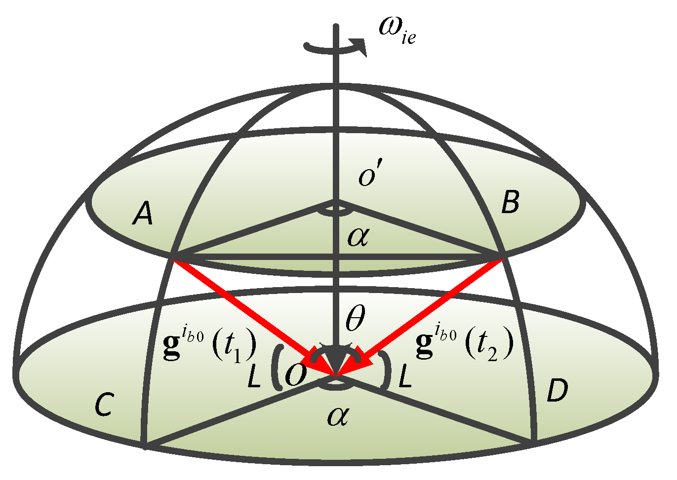
As shown in Figure 1, Point $O^{\prime }$ is the center of the latitude circle where the SINS is located. Point A and B are the positions in the inertial coordinate system at time $t_1$ and $t_2$ during the initial alignment, respectively. Point O is the intersection point of the vertical line of gravitational acceleration and the Earth’s axis [9]. ${\mathit{g}}^{i_{b0}}(t_1)$ and ${\mathit{g}}^{i_{b0}}(t_2)$ represent the gravitational acceleration vectors at $t_1$ and $t_2$, respectively. θ denotes the angle between the vector ${\mathit{g}}^{i_{b0}}(t_1)$ and ${\mathit{g}}^{i_{b0}}(t_2)$. $\alpha$ indicates the angle of the Earth turning around from $t_1$ to $t_2$. The angle between the latitude circle of point O and the vertical line of gravity is the latitude L.

The relationship between the lengths of the geometric line segments can be obtained as:

$$\left|AB\right|=2\left|AO\right|\cos L\sin \frac{\alpha }{2}$$

(1)

$$\left|AB\right|=2\left|AO\right|\sin \frac{\theta }{2}$$

(2)

The latitude value can be estimated by (1) and (2):

$$L=\arccos \left(\frac{\sin \frac{\theta }{2}}{\sin \frac{\alpha }{2}}\right)$$

(3)

The angular velocity ${\mathsf{\omega }}_{ie}$ of the Earth’s rotation is known; hence, the angle $\alpha$ of rotation can be expressed as follows:

$$\alpha ={\mathsf{\omega }}_{ie}(t_2-t_1)$$

(4)

To reduce the influence of the actual inertial navigation specific force measurement noise and the interference movement of the base, the angle is generally calculated after smoothing with the specific force integral over a period of time. Then, it can be obtained as:

$$\theta =a\cos \left[\frac{{({\mathit{v}}_1^{i_{b0}})}^T{\mathit{v}}_2^{i_{b0}}}{\sqrt{{({\mathit{v}}_1^{i_{b0}})}^T{\mathit{v}}_1^{i_{b0}}{({\mathit{v}}_2^{i_{b0}})}^T{\mathit{v}}_2^{i_{b0}}}}\right]$$

(5)

where ${\mathit{v}}_1^{i_{b0}}={\displaystyle {\int }_{t_1}^{t_1+\Delta t}{\mathit{g}}^{i_{b0}}(t)dt}$, ${\mathit{v}}_2^{i_{b0}}={\displaystyle {\int }_{t_2}^{t_2+\Delta t}{\mathit{g}}^{i_{b0}}(t)dt}$, $\Delta t$ indicates the integration time. ${\mathit{g}}^{i_{b0}}(t)$ is calculated as:

$${\mathit{g}}^{i_{b0}}(t)={\mathit{C}}_b^{i_{b0}}{\mathit{g}}^b(t)=-{\mathit{C}}_b^{i_{b0}}{\mathit{f}}^b(t)$$

(6)

where ${\mathit{g}}^b(t)$ is the gravitational acceleration vector in b coordinate system at time t. ${\mathit{f}}^b(t)$ is the measurement value of ${\mathit{g}}^b(t)$. ${\mathit{C}}_b^{i_{b0}}$ can be updated by measuring the gyroscope information in real-time:

$${\dot{\mathit{C}}}_b^{i_{b0}}={\mathit{C}}_b^{i_{b0}}\left({\mathit{\omega }}_{ib}^b\times \right)$$

(7)

where ${\mathit{\omega }}_{ib}^b$ is the output value of gyroscope and $\left({\mathit{\omega }}_{ib}^b\times \right)$ denotes the antisymmetric matrix of ${\mathit{\omega }}_{ib}^b$.

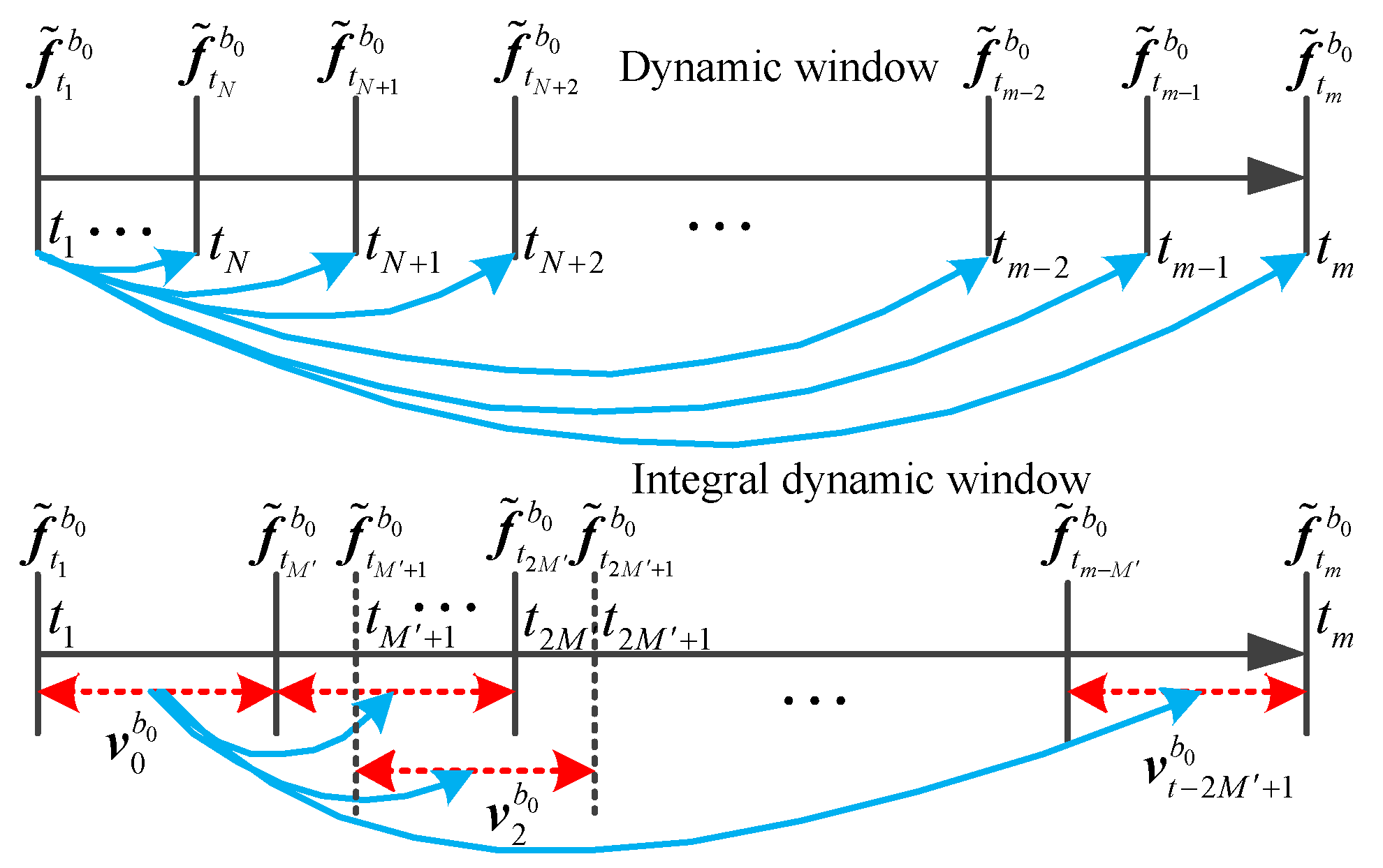
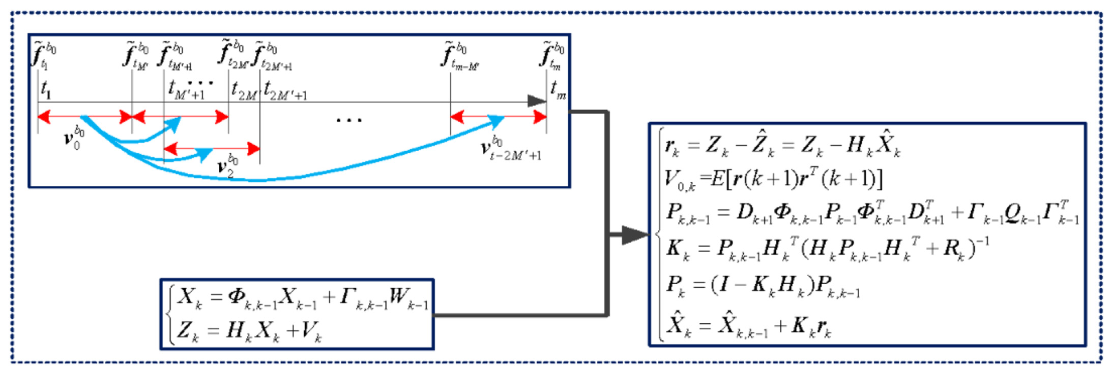
Hence, the key to latitude estimation is to extract more accurate ${\mathit{g}}^{i_{b0}}$ in real-time. However, under the in-motion condition, besides its instrument error, the accelerometer is also disturbed by the line vibration. This leads to a large output error of the accelerometer, which has a large impact on the latitude estimation. In this paper, a method of latitude estimation based on IDW-PF under the in-motion condition is proposed. The algorithm diagram is shown in Figure 2 [24].

In Figure 2, $-{\mathit{f}}^{i_{b0}}(t_N)$ indicates the calculated gravitational acceleration projected on the inertial coordinate system at time $t_N$. It can be calculated by updating the accelerometer output ${\tilde{\mathit{f}}}^{i_b}$ and the gyroscope output ${\tilde{\mathit{\omega }}}_{ib}^b$ at the current time. According to (3)–(7), take ${\tilde{\mathit{f}}}^{i_{b0}}(t_1)$ obtained from the calculation value at time $t_1$ as a reference. The real-time latitude estimation value at time $t_N$ can be obtained from the calculation value ${\tilde{\mathit{f}}}^{i_{b0}}(t_i)$ at $t_i(i=N,N+1,\cdots ,m)$ and ${\tilde{\mathit{f}}}^{i_{b0}}(t_1)$ at time $t_1$. That is, as long as there is the output of inertial instrument data, the current latitude estimation value can be obtained. The principle of integral dynamic window (IDW) is similar to that of dynamic window (DW).

In summary, the latitude estimation algorithm based on IDW-PF under the in-motion condition can be summarized as follows:

(1)

The integral value ${\mathit{v}}_0^{i_{b_0}}$ of time period $t_1\sim t_{M^{\prime }}$ is calculated according to ${\mathit{v}}_0^{i_{b_0}}={\displaystyle {\int }_{t_1}^{t_{M^{\prime }}}{\mathit{g}}^{i_{b_0}}(t)dt}$, which is used as the reference of the IDW.

(2)

Calculate the integral value of ${\mathit{v}}_0^{i_{b_0}}={\displaystyle {\int }_{t_{M^{\prime }+i}}^{t_{2M^{\prime }+i}}{\mathit{g}}^{i_{b_0}}(t)dt}$ time period $t_{M^{\prime }+i}\sim t_{2M^{\prime }+i}(i=0,1,\dots ,m-2M^{\prime }+1)$.

(3)

Perform polynomial fitting with time t as the independent variable to the calculation result of ${\mathit{v}}_0^{i_{b_0}}$ and ${\mathit{v}}_i^{i_{b_0}}$, namely ${\mathit{v}}_i^{i_{b_0}}=a_0+a_{1}t+a_2{t}^2+a_3{t}^3$.

(4)

The angle θ at time $t_{2M^{\prime }}$ can be obtained from the integral value ${\mathit{v}}_i^{i_{b_0}}$ of time period $t_{M^{\prime }+i}\sim t_{2M^{\prime }+i}(i=0,1,\dots ,m-2M^{\prime }+1)$ and ${\mathit{v}}_0^{i_{b_0}}$ of time period $t_1\sim t_{M^{\prime }}$ by using (5).

(5)

Calculate the angle α at time $t_{2M^{\prime }}$ by using (4).

(6)

The real-time latitude estimation value at time $t_{2M^{\prime }}$ can be obtained by using (3).

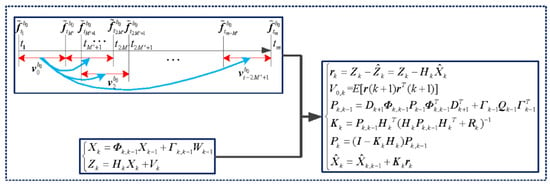
3. The Improved Kalman Filtering Algorithm

The state equation and observation equation of the stochastic linear discrete system are given as [25]:

$$\{\begin{array}{l}{\mathit{X}}_k={\mathit{\Phi }}_{k,k-1}{\mathit{X}}_{k-1}+{\mathit{\Gamma }}_{k,k-1}{\mathit{W}}_{k-1}\hfill \\ {\mathit{Z}}_k={\mathit{H}}_k{\mathit{X}}_k+{\mathit{V}}_k\hfill \end{array}$$

(8)

where ${\mathit{X}}_k$ is the state matrix at $t_k$, ${\mathit{\Phi }}_{k,k-1}$ is the one-step transition matrix from $t_{k-1}$ to $t_k$, ${\mathit{\Gamma }}_{k,k-1}$ is the system noise driving matrix, ${\mathit{Z}}_k$ is the system measurement sequence, ${\mathit{H}}_k$ is the measurement matrix, ${\mathit{V}}_k$ is the measurement noise sequence and ${\mathit{W}}_k$ is the system incentive noise sequence.

The standard KF recursive equations are as follows [26]:

(1)

State one-step prediction

$${\hat{\mathit{X}}}_{k,k-1}={\mathit{\Phi }}_{k,k-1}{\hat{\mathit{X}}}_{k-1}$$

(9)

(2)

State estimation

$${\hat{\mathit{X}}}_k={\hat{\mathit{X}}}_{k,k-1}+{\mathit{K}}_k({\mathit{Z}}_k-{\mathit{H}}_k{\hat{\mathit{X}}}_{k,k-1})$$

(10)

(3)

Filter gain

$${\mathit{K}}_k={\mathit{P}}_{k,k-1}{\mathit{H}}_k{}^T{({\mathit{H}}_k{\mathit{P}}_{k,k-1}{\mathit{H}}_k{}^T+{\mathit{R}}_k)}^{-1}$$

(11)

(4)

One-step prediction mean square error

$${\mathit{P}}_{k,k-1}={\mathit{\Phi }}_{k,k-1}{\mathit{P}}_{k-1}{\mathit{\Phi }}_{k,k-1}^T+{\mathit{\Gamma }}_{k-1}{\mathit{Q}}_{k-1}{\mathit{\Gamma }}_{k-1}^T$$

(12)

(5)

Estimated mean square error

$${\mathit{P}}_k=(\mathit{I}-{\mathit{K}}_k{\mathit{H}}_k){\mathit{P}}_{k,k-1}$$

(13)

where ${\hat{\mathit{X}}}_{k,k-1}$ is the state one-step prediction matrix, ${\hat{\mathit{X}}}_{k-1}$ is the estimated state matrix at $t_{k-1}$, ${\hat{\mathit{X}}}_k$ is the estimated state matrix at $t_k$, ${\mathit{K}}_k$ is the filter gain matrix, ${\mathit{P}}_{k,k-1}$ is the one-step prediction mean square error matrix, ${\mathit{R}}_k$ is the measurement noise variance matrix, ${\mathit{P}}_{k-1}$ is the error covariance matrix of the optimal filter value at $t_{k-1}$, ${\mathit{Q}}_{k-1}$ is system noise variance matrix at $t_{k-1}$, ${\mathit{P}}_k$ is the estimated mean square error matrix and $\mathit{I}$ is the unit matrix.

During the calculation process of KF, filtering anomalies or even divergences often occur. The main reasons are the inaccurate system models, the inaccurate noise statistical models, the accumulation of the rounding errors, etc. They cause the current measurement value to reduce the correction effect of the estimation value and the old measurement value to increase the correction effect of the estimation value [27]. The proposed IKF introduces a diagonal matrix fading factor into (12) so that the residual sequences at different times remain orthogonal everywhere, namely

$${\mathit{P}}_{k,k-1}={\mathit{D}}_{k+1}{\mathit{\Phi }}_{k,k-1}{\mathit{P}}_{k-1}{\mathit{\Phi }}_{k,k-1}^T{\mathit{I}}_{k+1}^T+{\mathit{\Gamma }}_{k-1}{\mathit{Q}}_{k-1}{\mathit{\Gamma }}_{k-1}^T$$

(14)

where ${\mathit{D}}_{k+1}$ is the diagonal matrix with multiple fading factors, and it can be determined by the following method [27]:

$${\mathit{D}}_{k+1}=diag[\begin{array}{cccc}{\lambda }_1(k+1)& {\lambda }_2(k+1)& \cdots & {\lambda }_n(k+1)\end{array}]$$

(15)

$${\lambda }_n(k+1)=\{\begin{array}{cc}{\alpha }_k\cdot C_k& {\alpha }_k\cdot C_k\ge 1\\ 1& {\alpha }_k\cdot C_k<1\end{array}$$

(16)

where ${\alpha }_k\ge 1(k=1,2,\cdots ,n)$ are the coefficients predetermined by the prior knowledge. It can increase the corresponding ${\alpha }_k$ of the components that are prone to sudden changes. If the system has no prior knowledge, take ${\alpha }_k=1$. In (16), $C_k$ can be expressed as

$$C_k=\frac{tr[{\mathit{N}}_k]}{{\displaystyle \sum _{i=1}^n{\alpha }_i{\mathit{M}}_k}}$$

(17)

where $tr[·]$ denotes the trace of the matrix “$·$”. ${\mathit{N}}_k={\mathit{V}}_{0,k}-{\mathit{H}}_k{\mathit{Q}}_k{\mathit{H}}_k^T-l_k{\mathit{R}}_k$, $l_k\ge 1$, and it is the weakening factor. ${\mathit{V}}_{0,k}$ is the mean square error. ${\mathit{M}}_K={\mathit{H}}_k{\mathit{\Phi }}_{k,k-1}{\mathit{P}}_{k-1}{\mathit{\Phi }}_{k,k-1}^T{\mathit{H}}_k^T$. The multi-fading factor KF is used to fade each data channel at different rates. It can better adjust the gain matrix. Even when the system reaches a steady state, the gain matrix can be adjusted adaptively to enhance the robustness of the model mismatch and the system destabilization. More accurate and stable estimation results will be obtained.

4. The Proposed In-Motion Alignment Method

The IKF-based alignment technology for SINS requires auxiliary navigation equipment to complete the alignment. Considering that the external velocity of the vehicle is easy to obtain, this paper focuses on the use of external reference velocity-aided alignment methods. The difference between the velocity output by SINS and the velocity provided by the auxiliary navigation equipment is used as the observation. Attitude misalignment angle and inertial device error are estimated by IKF so as to complete the initial alignment.

The instability of the vertical channel is considered; the upward velocity and the z-axis accelerometer constant bias are not regarded as the state variables in this paper. Hence, the state vectors selected in the study are as follows:

$$\mathit{X}(t)={[\delta V_E,\delta V_N,{\varphi }_E,{\varphi }_N,{\varphi }_U,\delta L,\delta \lambda ,{\nabla }_x,{\nabla }_y,{\epsilon }_x,{\epsilon }_y,{\epsilon }_z]}^T$$

(18)

where $\delta V_E$ is the eastward velocity error, $\delta V_N$ is the northward velocity error, ${\varphi }_E$ is the eastward misalignment angle, ${\varphi }_N$ is the northward misalignment angle, ${\varphi }_U$ is the upward misalignment angle, $\delta L$ is the latitude error, $\delta \lambda$ is the longitude error, ${\nabla }_x$ is the x-axis accelerometer bias, ${\nabla }_y$ is the y-axis accelerometer bias, ${\epsilon }_x$ is the x-axis gyroscope constant drift, ${\epsilon }_y$ is the y-axis gyroscope constant drift and ${\epsilon }_z$ is the z-axis gyroscope constant drift.

The state equation of the system is expressed as [28,29]:

$$\dot{\mathit{X}}(t)=\mathit{F}(t)\mathit{X}(t)+\mathit{G}(t)\mathit{w}(t)$$

(19)

where $\mathit{X}(t)$ is the system state vector, $\mathit{F}(t)$ is the system matrix, $\mathit{G}(t)$ is the system noise matrix and $\mathit{w}(t)$ is the system noise vector. The system matrix $\mathit{F}(t)$ is expressed as:

$$\mathit{F}(t)=\left[\begin{array}{cc}\mathit{T}(t)& \mathit{M}(t)\\ {\mathit{0}}_{5\times 9}& {\mathit{0}}_{5\times 3}\end{array}\right]$$

(20)

where $\mathit{M}(t)={[{\mathit{0}}_{3\times 2}{\mathit{C}}_n^b{\mathit{0}}_{3\times 2}]}^T$.

$$\mathit{T}(t)=\left[\begin{array}{ccccccccc}{T}_{11}& T_{12}& 0& -f_U& f_N& T_{16}& 0& C_b^n(1,1)& C_b^n(1,2)\\ T_{21}& -\frac{V_U}{R_n}& f_U& 0& -f_E& T_{26}& 0& C_b^n(2,1)& C_b^n(2,2)\\ 0& -\frac{1}{R_n}& 0& T_{34}& {{\rm T}}_{35}& 0& 0& 0& 0\\ \frac{1}{R_e}& 0& T_{43}& 0& -\frac{V_N}{R_n}& -{\omega }_{ie}\sin L& 0& 0& 0\\ \frac{\tan L}{R_e}& 0& T_{53}& 0& \frac{V_U}{R_n}& T_{56}& 0& 0& 0\\ 0& \frac{1}{R_n}& 0& 0& 0& 0& 0& 0& 0\\ \frac{1}{R_e\cos L}& 0& 0& 0& 0& \frac{V_E\tan L}{R_e\cos L}& 0& 0& 0\end{array}\right]$$

(21)

where $L$ is the latitude, $f_E$, $f_N$ and $f_U$ are the eastward acceleration, northward acceleration and upward acceleration, respectively. $V_E$, $V_N$ and $V_U$ are the eastward velocity, northward velocity and upward velocity, respectively. ${\omega }_{ie}$ is the angular velocity of the Earth’s rotation. $R_e$ is the Earth’s semi-major axis, and $R_n$ is the radius of principal curvature. ${\mathit{C}}_b^n$ is the attitude matrix, and all nonzero elements of the matrix T(t) are expressed as: $T_{11}=\frac{V_N\tan L-V_U}{R_e}$, $T_{12}=2({\omega }_{ie}\sin L+\frac{V_E\tan L}{R_e})$, $T_{16}=2{\omega }_{ie}(V_U\sin L+V_N\cos L)+\frac{V_E{V}_N}{R_e{(\cos L)}^2}$, $T_{21}=-2({\omega }_{ie}\sin L+\frac{V_E\tan L}{R_e})$, $T_{26}=-(2{\omega }_{ie}\cos L+\frac{V_E}{R_e{(\cos L)}^2})V_E$, $T_{34}={\omega }_{ie}\sin L+\frac{V_{E}tanL}{R_e}$, ${{\rm T}}_{35}=-({\omega }_{ie}\cos L+\frac{V_E}{R_e})$, $T_{43}=-({\omega }_{ie}\sin L+\frac{V_E\tan L}{R_e})$, $T_{53}={\omega }_{ie}\cos L+\frac{V_E}{R_e}$, $T_{56}={\omega }_{ie}\cos L+\frac{V_E}{R_e{(cosL)}^2}$.

The horizontal velocity of the SINS is assumed to be expressed as [30]:

$$\{\begin{array}{l}{V}_{ES}=V_{ET}+\delta V_{ES}\\ V_{NS}=V_{NT}+\delta V_{NS}\end{array}$$

(22)

where $V_{ES}$ and $V_{NS}$ are the eastward velocity and the northward velocity of the SINS, respectively. $V_{ET}$ and $V_{NT}$ are the true eastward velocity and northward velocity of the carrier, respectively. $\delta V_{ES}$ and $\delta V_{NS}$ are the eastward velocity error and the northward velocity error of the SINS, respectively.

The external reference velocity is assumed to be expressed as [30]:

$$\{\begin{array}{l}{V}_{ED}=V_{ET}+\delta V_{ED}\\ V_{ND}=V_{NT}+\delta V_{ND}\end{array}$$

(23)

where $V_{ED}$ and $V_{ND}$ are the eastward velocity and the northward velocity of the external equipment, respectively. $\delta V_{ED}$ and $\delta V_{ND}$ are the eastward velocity error and the northward velocity error of the external equipment, respectively.

Hence, the measurement equation of the system can be expressed as:

$${\mathit{Z}}_k=\left[\begin{array}{l}{V}_{ES}-V_{ED}\\ V_{NS}-V_{ND}\end{array}\right]=\left[\begin{array}{l}\delta V_{ES}-\delta V_{ED}\\ \delta V_{NS}-\delta V_{ND}\end{array}\right]={\mathit{H}}_k{\mathit{X}}_k+{\mathit{V}}_k$$

(24)

where ${\mathit{H}}_k=\left[\begin{array}{cc}1& 0\\ 0& 1\end{array}{\mathbf{0}}_{2\times 10}\right]$.

So far, the model of velocity-aided in-motion alignment has been established. Then, the IKF can be used for filtering, and the process is introduced as follows:

(1)

State prediction

$${\mathit{r}}_k={\mathit{Z}}_k-{\widehat{\mathit{Z}}}_k={\mathit{Z}}_k-{\mathit{H}}_k{\widehat{\mathit{X}}}_k$$

(25)

(2)

Calculate the diagonal matrix with multiple suboptimal fading factors, where

$${\mathit{V}}_{0,k}=E[\mathit{r}(k+1){\mathit{r}}^T(k+1)]=\{\begin{array}{cc}\mathit{r}(1){\mathit{r}}^T(1)& k=0\\ \frac{\rho {\mathit{V}}_{0,k-1}+{\mathit{r}}_k{\mathit{r}}_k^T}{1+\rho }& k\ge 1\end{array}$$

(26)

where $0\le \rho \le 1$, and it is the forgetting factor.

(3)

Calculate the prediction state covariance matrix using (14).

(4)

Calculate the gain matrix using (11).

(5)

Calculate the state estimation and its covariance matrix at t.

$$\{\begin{array}{c}{\mathit{P}}_k=(\mathit{I}-{\mathit{K}}_k{\mathit{H}}_k){\mathit{P}}_{k,k-1}\\ {\widehat{\mathit{X}}}_k={\widehat{\mathit{X}}}_{k,k-1}+{\mathit{K}}_k{\mathit{r}}_k\end{array}$$

(27)

At this point, the in-motion alignment method based on IKF under geographic latitude uncertainty has been implemented. Then the initial attitude can be obtained.

5. Simulation Results and Discussions

In order to verify the latitude estimation and in-motion alignment method proposed in this paper, firstly, the simulation experiments of the latitude estimation based on the IDW-PF are carried out. Then, the simulation experiments of in-motion alignment based on the IKF are performed for various motion paths. The external reference velocity error is not considered when studying the influence of different maneuver tracks on the in-motion alignment; here, the external reference velocity error is set to zero. The latitude used in the simulation experiment is the latitude estimation value based on the IDW-PF.

The specifications of the inertial measurement unit (IMU) are listed in

Table 1. Parameters settings of IMU.

Coordinate Axis	Gyroscope		Accelerometer
	$\mathbf{Constant}\mathbf{Drift}\mathbf{(}°\mathbf{/}\mathbf{h}\mathbf{)}$	$\mathbf{Random}\mathbf{Drift}(°/\sqrt{\mathbf{h}})$	$\mathbf{Constant}\mathbf{Bias}\left(\mathsf{\mu }\mathbf{g}\right)$	$\mathbf{Random}\mathbf{Walk}\left(\mathsf{\mu }\mathbf{g}\right)$
x-axis	0.02	0.02	50	50
y-axis	0.02	0.02	50	50
z-axis	0.02	0.02	50	50

. The instrument output frequency is 200 Hz. At the time of the experiment, the system has completed the coarse alignment, and the pitch, roll and heading attitude errors at the beginning of fine alignment are ${0.1}^{°}$, ${0.1}^{°}$ and $1^{°}$, respectively. The linear velocity of the carrier is 2 m/s; the turn angle rate is ${0.9}^{°}/\mathrm{s}$. The simulation time of latitude estimation and in-motion are set as 300 s and 900 s, respectively. The time parameters are set as: $t_N=8\mathrm{s}$ and $t_{M^{\prime }}=4\mathrm{s}$.

5.1. Simulation Experiment of the Latitude Estimation Based on the IDW-PF

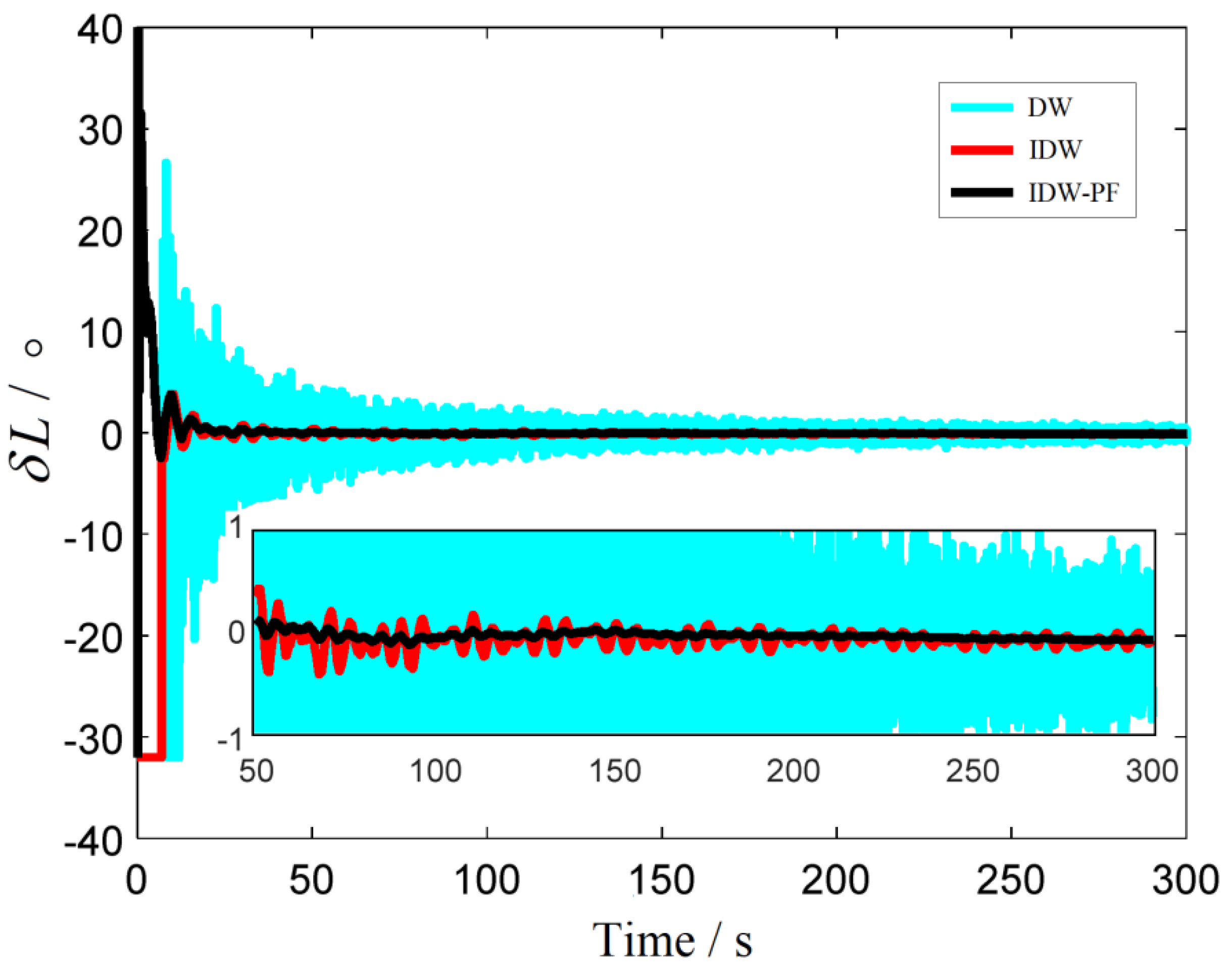
In this subsection, three kinds of latitude estimation algorithms are performed, which are based on the DW, IDW and IDW-PF, respectively. Figure 3 shows the curves of the latitude estimation error, $\delta L$ denotes the latitude error, and the statistical results of the latitude estimation error are listed in

Table 2. Statistical results of latitude estimation errors.

Latitude Estimation Algorithm	0~100 (s)		100~200 (s)		200~300 (s)
	Mean (°)	SD (°)	Mean (°)	SD (°)	Mean (°)	SD (°)
DW	3.638	9.286	0.175	0.772	−0.152	0.608
IDW	−3.424	8.853	−0.167	0.098	−0.099	0.062
IDW-PF	0.622	2.974	−0.031	0.016	−0.016	0.013

.

It can be seen from Figure 3 and Table 2 that all three methods can realize self-estimation of latitude. However, due to the influence of accelerometer noise, the standard deviation (SD) of the DW method is relatively large. The IDW method effectively suppresses the influence of the accelerometer noise on the estimation accuracy through the integral effect. The IDW-PF method achieves the second smoothing of the interference acceleration by performing the PF on the result of the specific force integration. Hence, the IDW-PF method has the best performance with the fastest convergence speed and the highest estimation accuracy.

5.2. Simulation Experiment of Alignment Based on IKF When the Carrier Performs Uniform Linear Motion

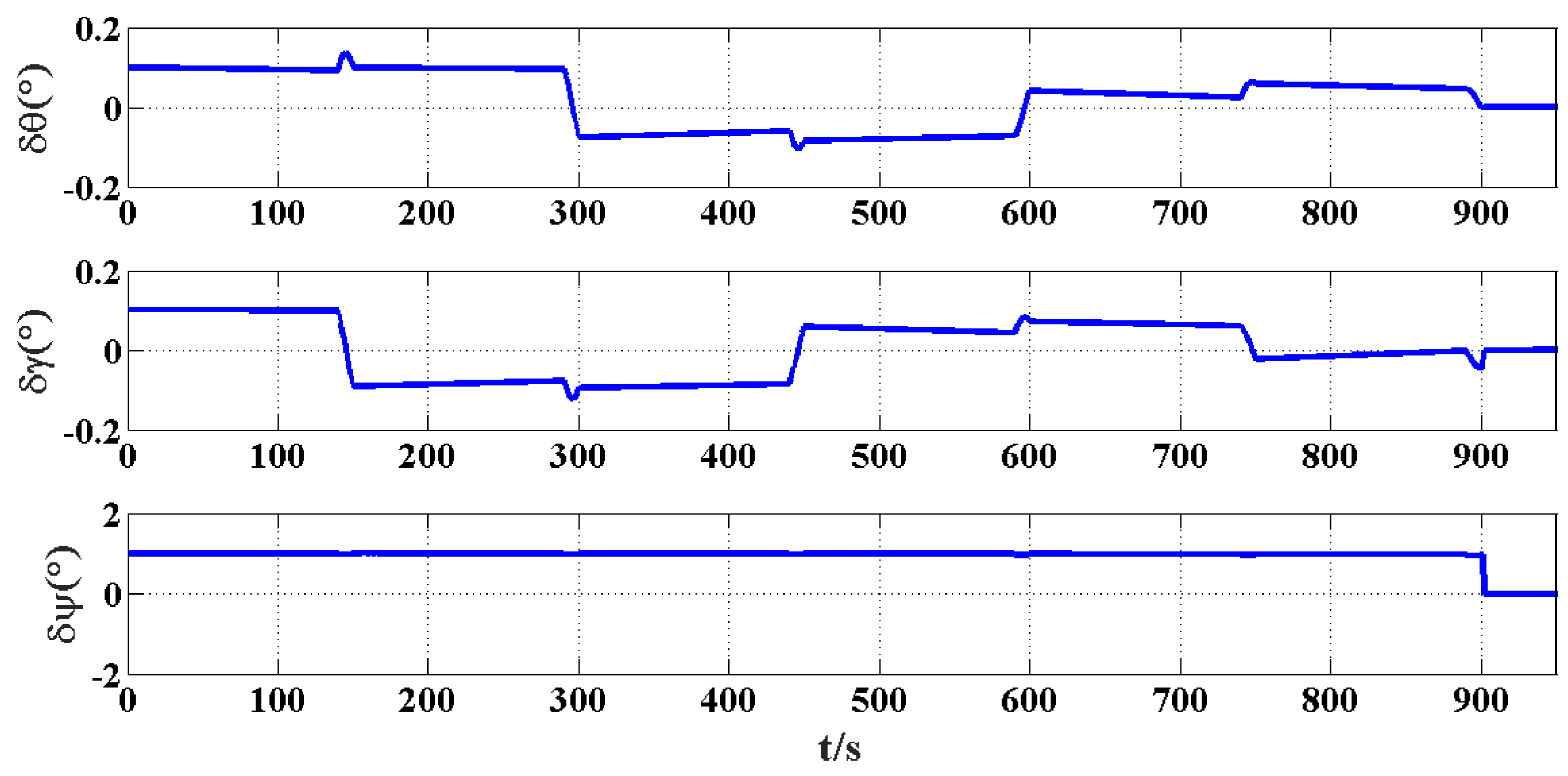
The initial attitude angles are assumed to be as follows: the pitch angle is $0^{°}$, the roll angle is $0^{°}$, the heading angle is $0^{°}$, ${90}^{°}$, ${180}^{°}$ and ${270}^{°}$. Figure 4 shows the attitude error of the in-motion alignment of uniform linear motion when the heading angle is ${90}^{°}$. Figure 5 shows the estimation values of the gyroscope and accelerometer constant error when the heading angle is ${90}^{°}$. $\delta \theta$, $\delta \gamma$ and $\delta \varphi$ are pitch error, roll error and heading error, respectively. ${\Delta }_x$ and ${\Delta }_y$ are accelerometer bias of x-axis and y-axis, respectively. ${\epsilon }_x$ and ${\epsilon }_y$ are gyroscope drift of x-axis and y-axis, respectively. The system is open-loop during the alignment process, the alignment ends at 900 s, and then the attitude is compensated.

Table 3. Statistical results of uniform linear motion.

Parameters	Initial Heading Angle (°)				Mean	SD
	0	90	180	270
$\delta \theta (°)$	0.0020	0.0011	0.0016	0.0028	0.0019	0.00072
$\delta \gamma (°)$	−0.0026	−0.0022	−0.0004	−0.0020	−0.0018	0.00097
$\delta \mathsf{\Psi } (°)$	0.0698	0.0345	−0.0576	0.0569	0.0259	0.0572
${\Delta }_x (\mathsf{\mu }\mathrm{g})$	1.556	1.036	1.353	0.8352	1.195	0.3215
${\Delta }_y (\mathsf{\mu }\mathrm{g})$	−1.512	−1.550	−1.967	−1.306	−1.584	0.2771
${\epsilon }_x (°/\mathrm{h})$	−0.010	0.073	0.013	0.066	0.0355	0.0405
${\epsilon }_y (°/\mathrm{h})$	0.010	0.011	0.036	−0.010	0.0117	0.0188

shows the statistical results of the attitude error, the estimation values of the gyroscope and accelerometer constant error when the heading angle is $0^{°}$, ${90}^{°}$, ${180}^{°}$ and ${270}^{°}$.

It can be seen from Figure 4 and Figure 5 and Table 3 that when the initial heading angle is 90°, the pitch, roll and heading errors measured at 900 s are sufficiently low and are 0.0011°, −0.0022° and 0.0345°, respectively. The bias of the x-axis and y-axis accelerometer is 1.036 µg and −1.550 µg, respectively. The constant drift of x-axis and y-axis gyroscopes is 0.073°/h and 0.011°/h, respectively. Although the alignment accuracy can meet the alignment requirements, there are large errors in estimating the accelerometer constant bias and gyroscope constant drift. It can be seen from Table 3 that the above conclusions are true for multiple heading angles. Moreover, the estimation accuracy of the misalignment angle is stable under the condition of uniform linear motion maneuvering.

5.3. Simulation Experiment of Alignment Based on IKF When the Carrier Performs Turning Maneuver (Circular Path)

The initial attitude angles are assumed to be as follows: the pitch angle is 0°, the roll angle is 0° and the heading angle is 0°. When the influence of the circular maneuver mode on the in-motion alignment is considered, the maneuvering trajectory is shown in Figure 6. 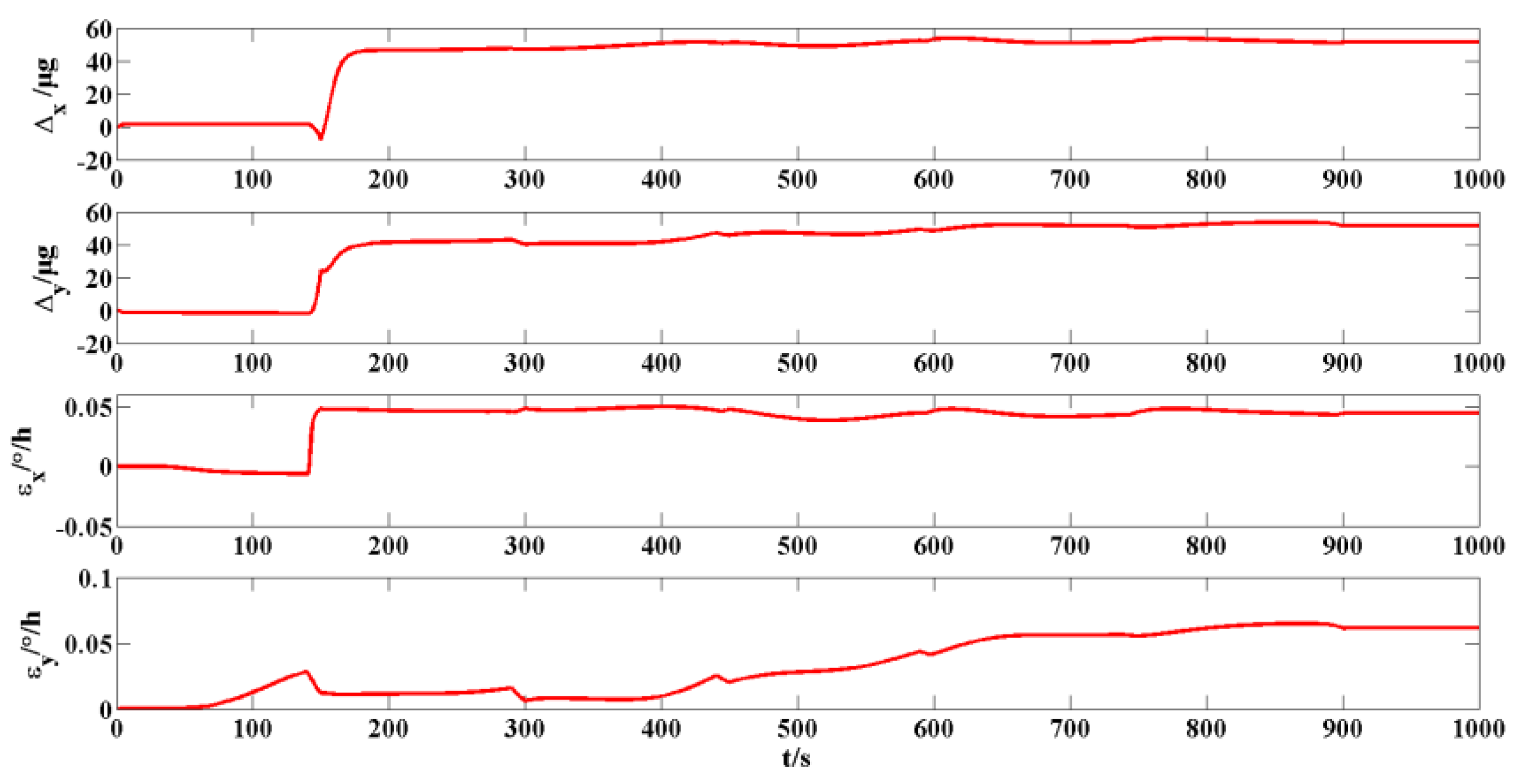The results of the attitude error and the constant error estimation for the gyroscope and accelerometer are shown in Figure 7 and Figure 8, respectively.

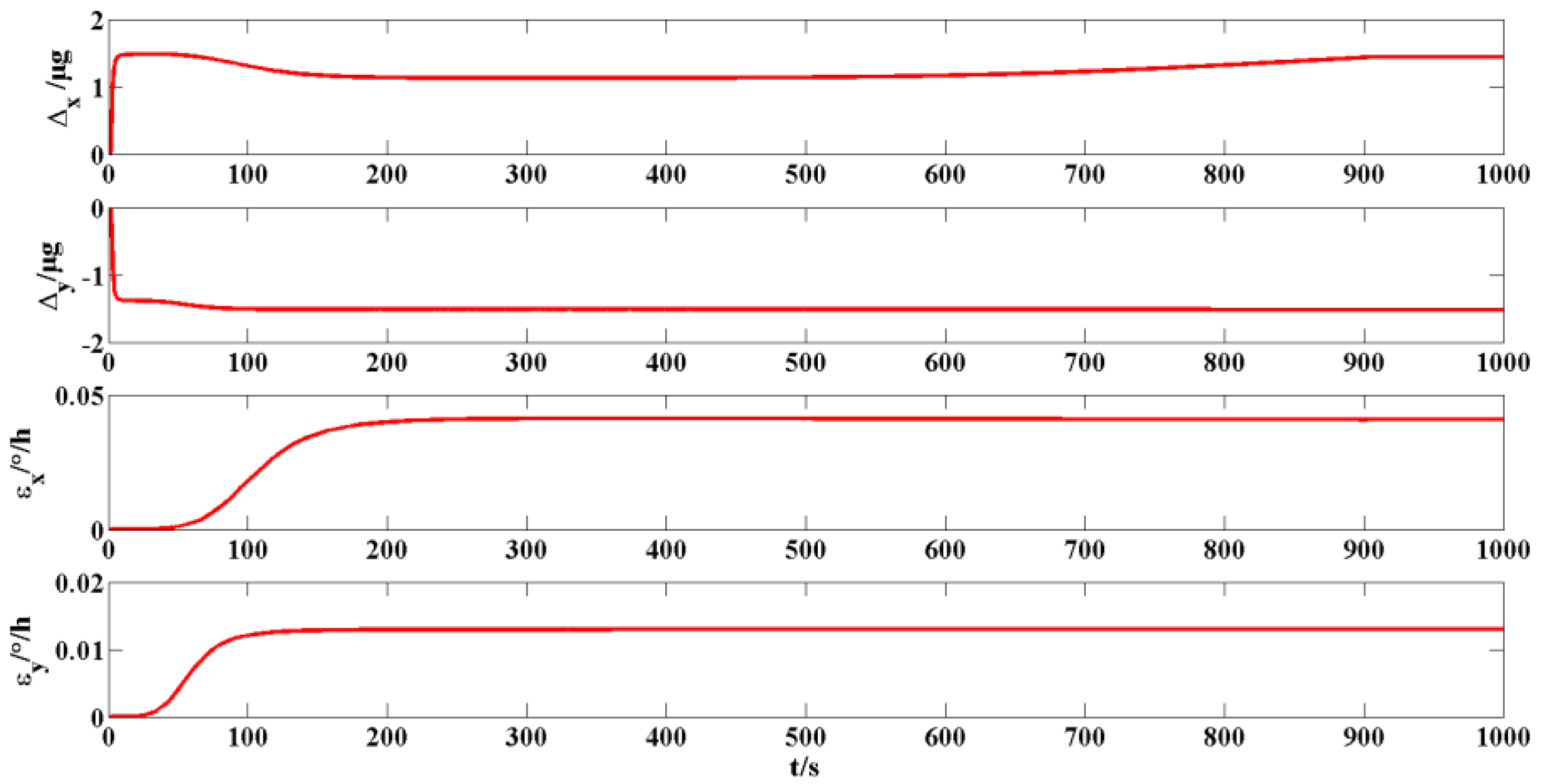
When the alignment ends at 900 s, the attitude error, accelerometer bias and gyroscope drift are measured. The pitch error is 0.0002°, the roll error is −0.0010° and the heading error is 0.0016°. The misalignment angle is estimated well in the maneuvering mode. The bias of the x-axis and y-axis accelerometer is 45.19 µg and 43.84 µg, respectively. Moreover, they are close to the bias value of 50 µg set by the simulation, which is explained that the accelerometer bias has been effectively estimated. The estimated constant drift of the x-axis and y-axis gyroscope is 0.043°/h and 0.061°/h, respectively. There is a certain gap between the constant drift of 0.006°/h set by the simulation, which is explained that the gyroscope constant drift is not well estimated.

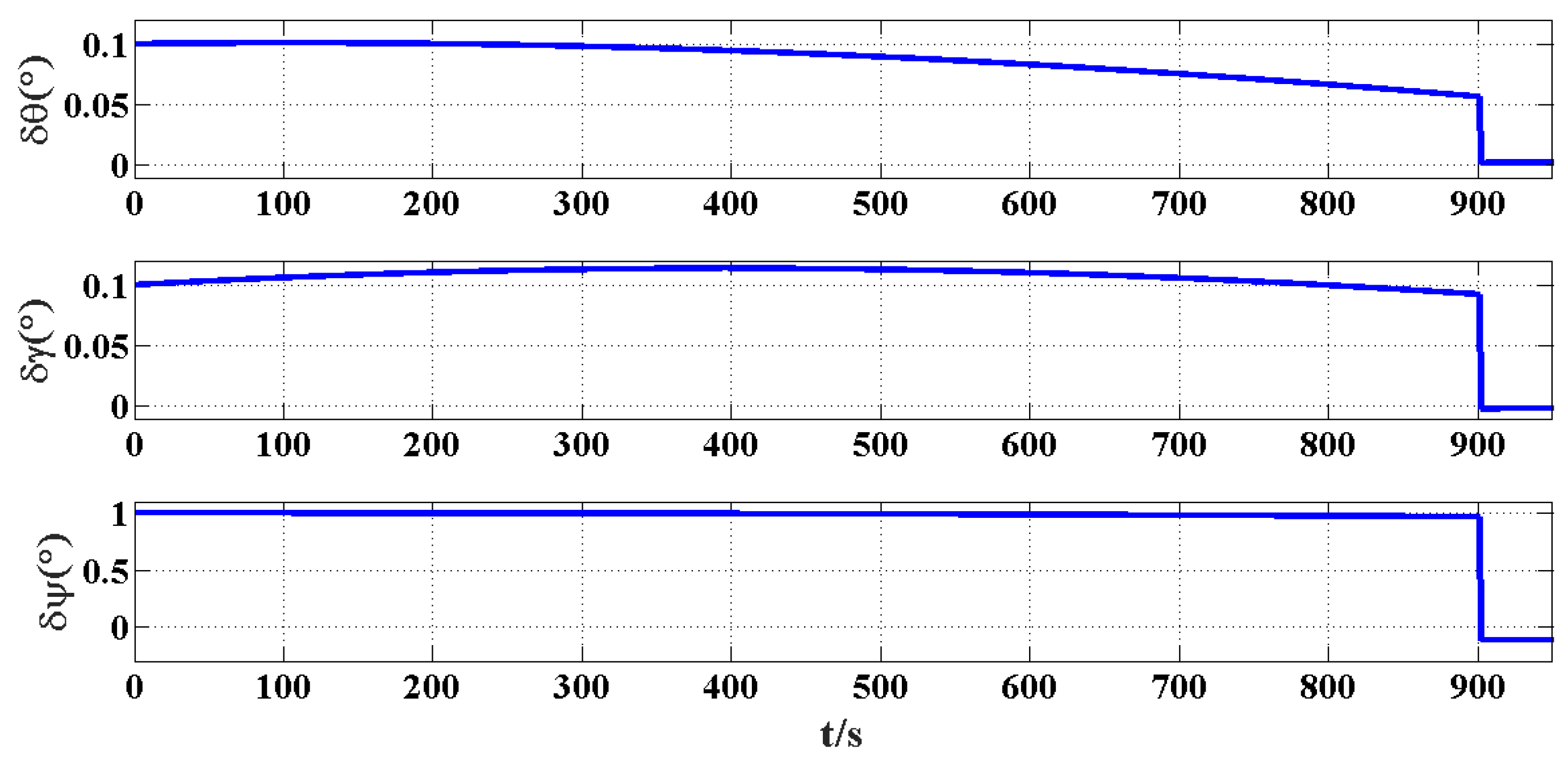
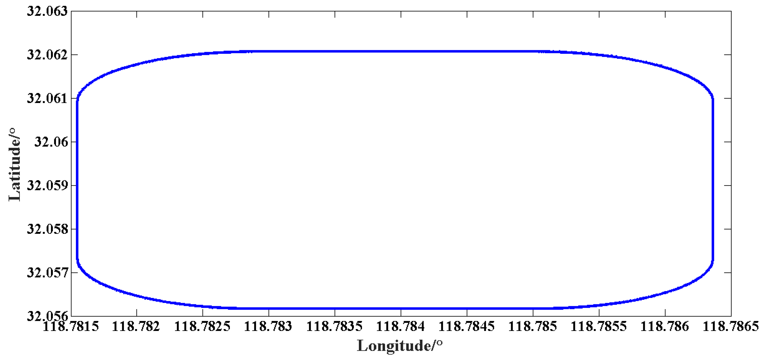
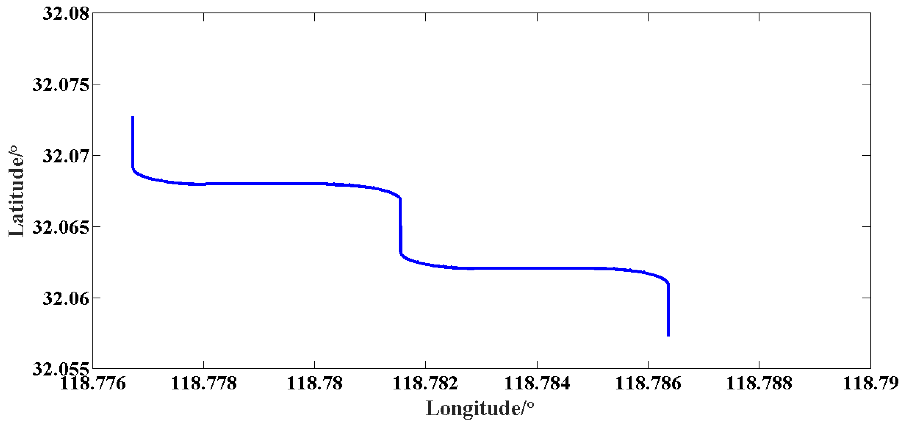
5.4. Simulation Experiment of Alignment Based on IKF When the Carrier Performs Turning Maneuver (Trapezoidal Path)

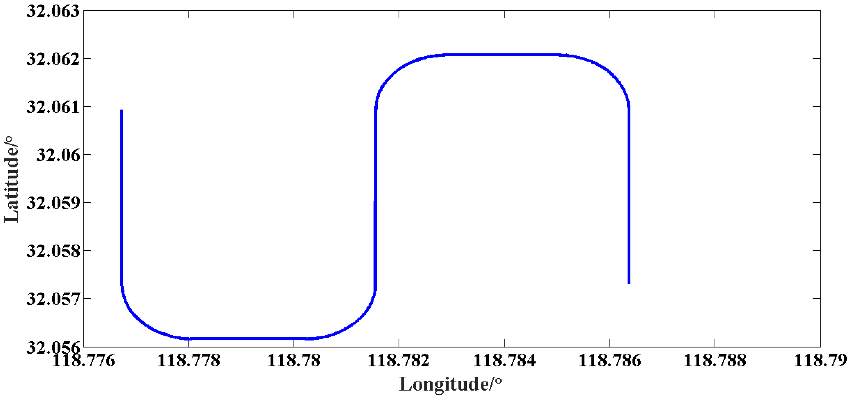
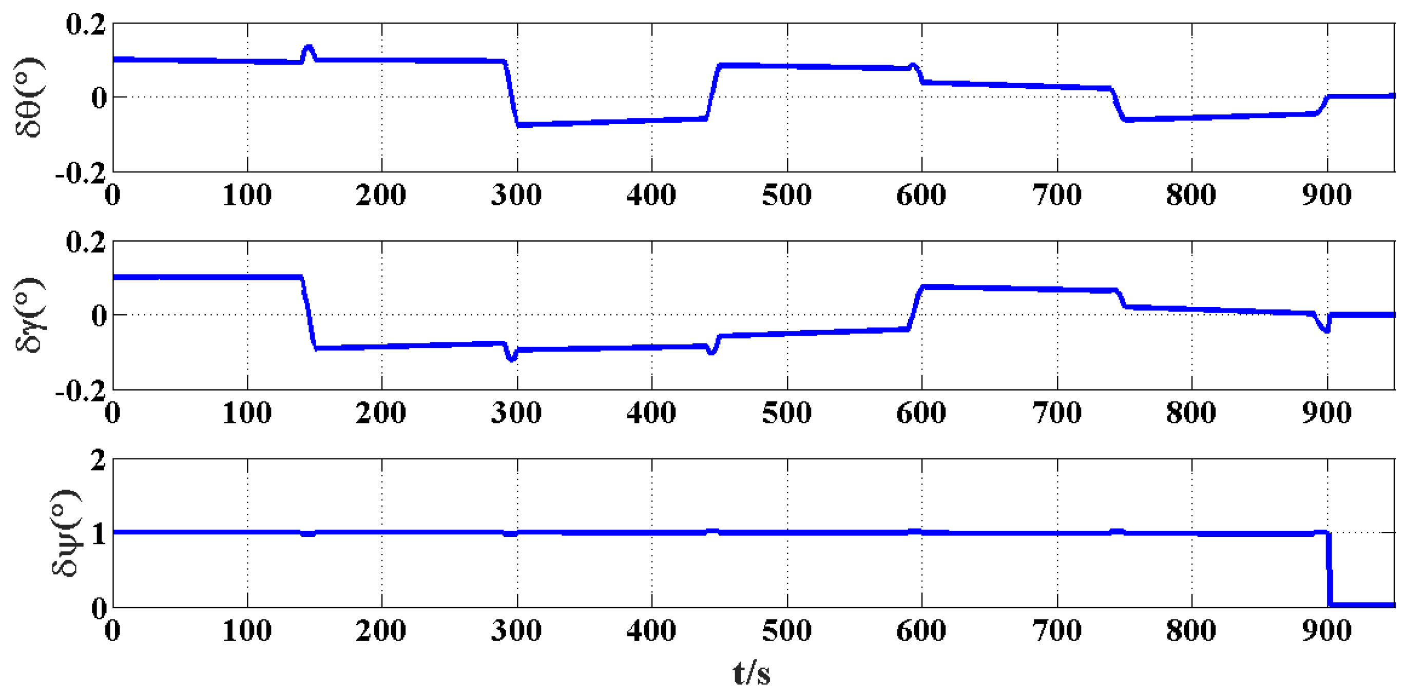
The initial attitude angles are assumed to be as follows: the pitch angle is 0°, the roll angle is 0° and the heading angle is 0°. When the influence of the trapezoidal maneuvering mode on the in-motion alignment is considered, the maneuvering trajectory is shown in Figure 9. 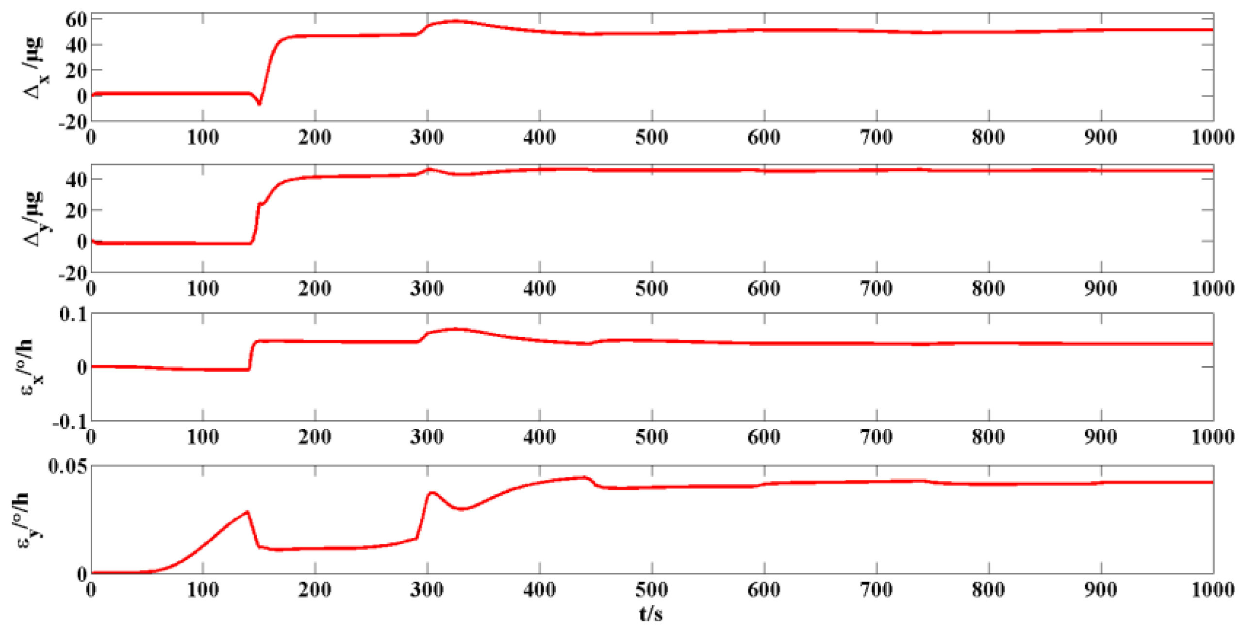The results of the attitude error and the constant error estimation for the gyroscope and accelerometer are shown in Figure 10 and Figure 11, respectively.

The attitude error, accelerometer bias and gyroscope drift were measured at 900 s. The pitch error is 0.0002°, the roll error is 0.0009° and the heading error is −0.0047°. The misalignment angle is estimated well in the maneuvering mode. The bias of the x-axis and y-axis accelerometer is 51.09 µg and 48.51 µg, respectively. Moreover, they are close to the bias value 50 µg set by the simulation, which is explained that the accelerometer bias was effectively estimated. The estimated constant drift of x-axis and y-axis gyroscopes is 0.0095°/h and 0.0096°/h, respectively. There is a certain gap between the constant drift of 0.006°/h set by the simulation, which shows that there is a certain error in the constant drift of the gyroscope estimated in the maneuvering mode.

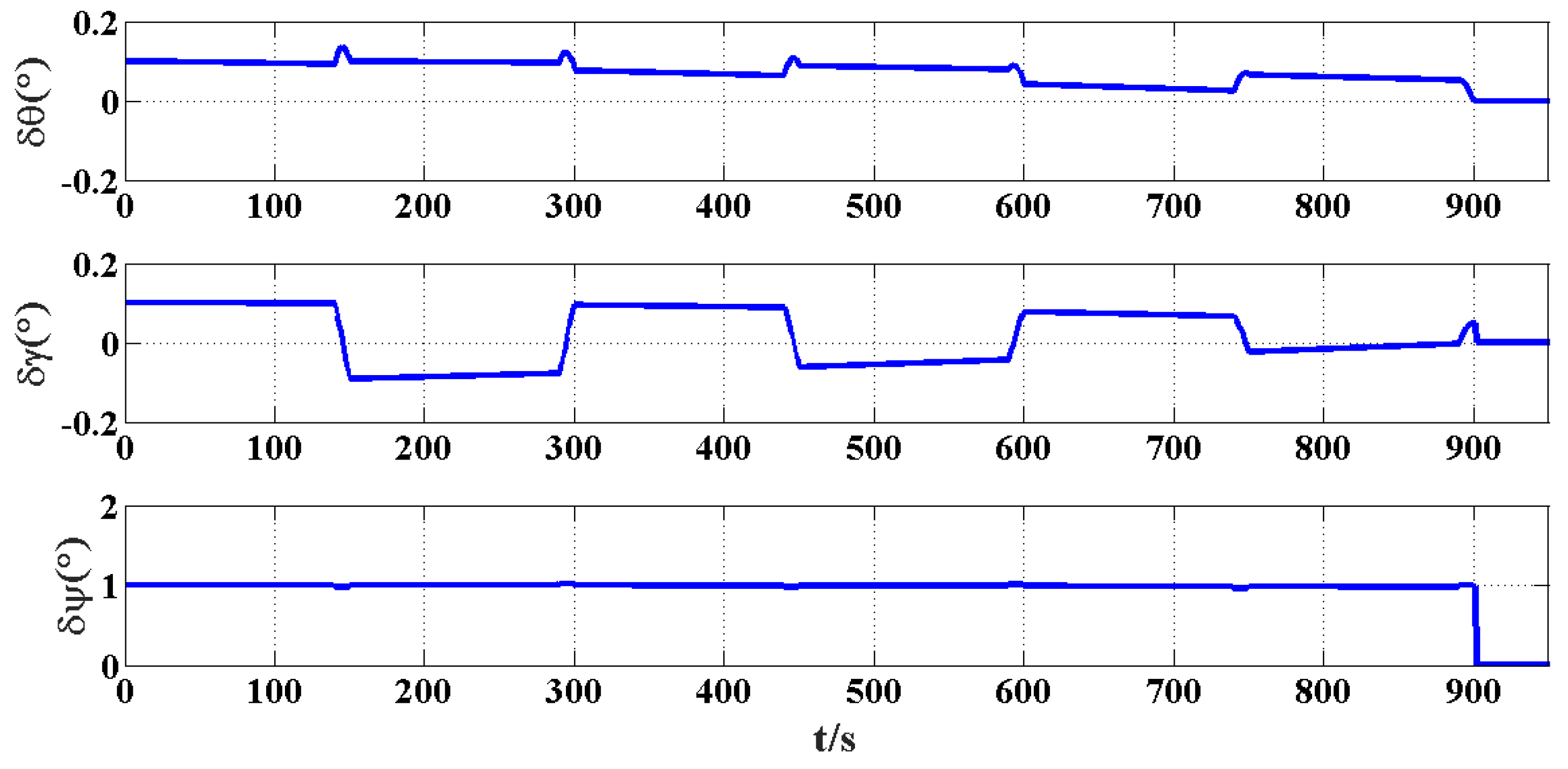
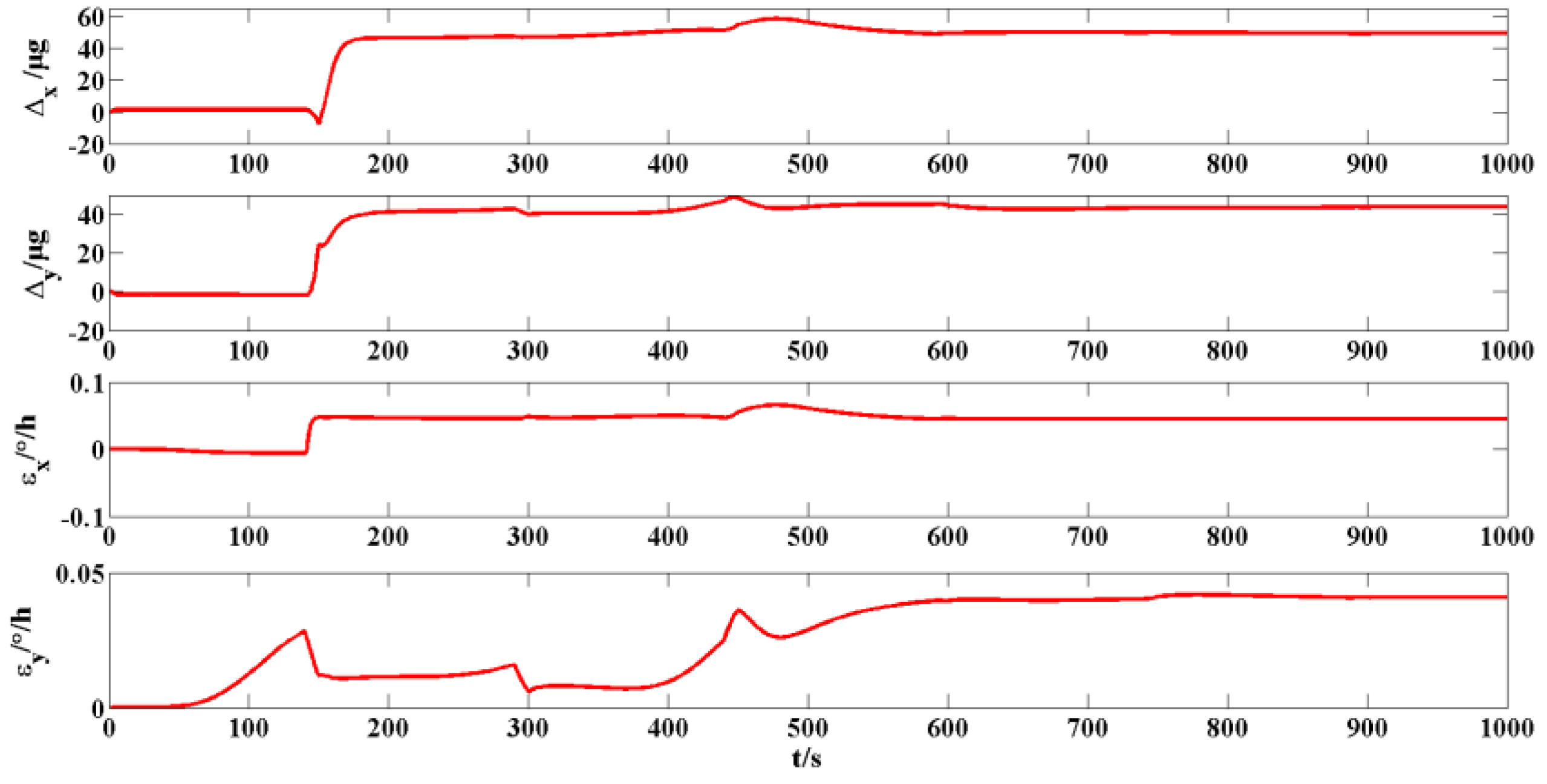
5.5. Simulation Experiment of Alignment Based on IKF When the Carrier Performs Turning Maneuver (S-Shaped Path)

The initial attitude angles are assumed to be as follows: the pitch angle is 0°, the roll angle is 0° and the heading angle is 0°. When the influence of the s-shaped maneuvering mode on the in-motion alignment is considered, the maneuvering trajectory is shown in Figure 12. The results of attitude error and constant error estimation for the gyroscope and accelerometer are shown in Figure 13 and Figure 14, respectively.

The pitch error is 0.0003°, the roll error is 0.0011° and the heading error is 0.0039° when the alignment ends at 900 s. The misalignment angle is estimated well in the maneuvering mode. The bias of the x-axis and y-axis accelerometer is 49.02 µg and 46.68 µg, respectively. Moreover, they are close to the bias value of 50 µg set by the simulation, which is explained that the accelerometer bias has been effectively estimated. The estimated constant drift of the x-axis and y-axis gyroscope is 0.0088°/h and 0.0022°/h, respectively. There is a certain gap between the constant drift of 0.006°/h set by the simulation, which shows that there is a certain error in the constant drift of the gyroscope estimated in the maneuvering mode.

The results of the alignment experiments between the three types of turning maneuvers are compared; it can be seen that, although the turning maneuver can have a positive effect on the estimation of the attitude misalignment angle and the IMU error, there are some differences in the effects of the motion path of the carrier, so the in-motion alignment effect is not only affected by the maneuver of the carrier but also by the path selection. Among the above three kinds of paths, the trapezoidal path has the best alignment effect, and the effect of the s-shaped path is better than that of the circular path. Hence, it is better to choose a trapezoidal path or an s-shaped path when practical conditions permit.

6. Conclusions

In-motion alignment method of SINS under geographic latitude uncertainty was proposed. The proposed method contains a method of latitude estimation and in-motion alignment method. Firstly, the latitude estimation algorithm based on the IDW-PT was designed. This IDW-PT can suppress and compensate for the interference of the carrier’s line vibration. Secondly, the in-motion alignment method based on the IKF was devised. The multi-fading factor is introduced into the KF to fade each data channel at different rates. The gain matrix can be adjusted adaptively to enhance the robustness of the model mismatch and system destabilization and accordingly achieve more accurate and stable estimation results. Finally, the simulation experiment was shown to prove that the proposed method can estimate the geographic latitude accurately and applies to the in-motion initial alignment. The mean and standard deviation of the estimated latitude can achieve −0.016° and 0.013° within 300 s. Under the turning maneuver conditions, the convergence accuracy and speed of the attitude misalignment angle and the inertial device error can be improved. Moreover, the trapezoidal path was shown to be the optimal maneuvering path. The pitch error is 0.0002°, the roll error is 0.0009° and the heading error is −0.0047° after the alignment ends at 900 s. Based on the simulation performance of the proposed method, it is expected to be applied in real-time application. The method can enhance the navigation performance and the dynamic performance of the carrier. In the future, further investigations should be developed for the more serious situation such as the large misalignment angle, non-horizontal path and multi-path combination.