
Three Decades of Gross Primary Production (GPP) in China: Variations, Trends, Attributions, and Prediction Inferred from Multiple Datasets and Time Series Modeling


 ,
,  ,
, 
Abstract
:
1. Introduction
2. Method
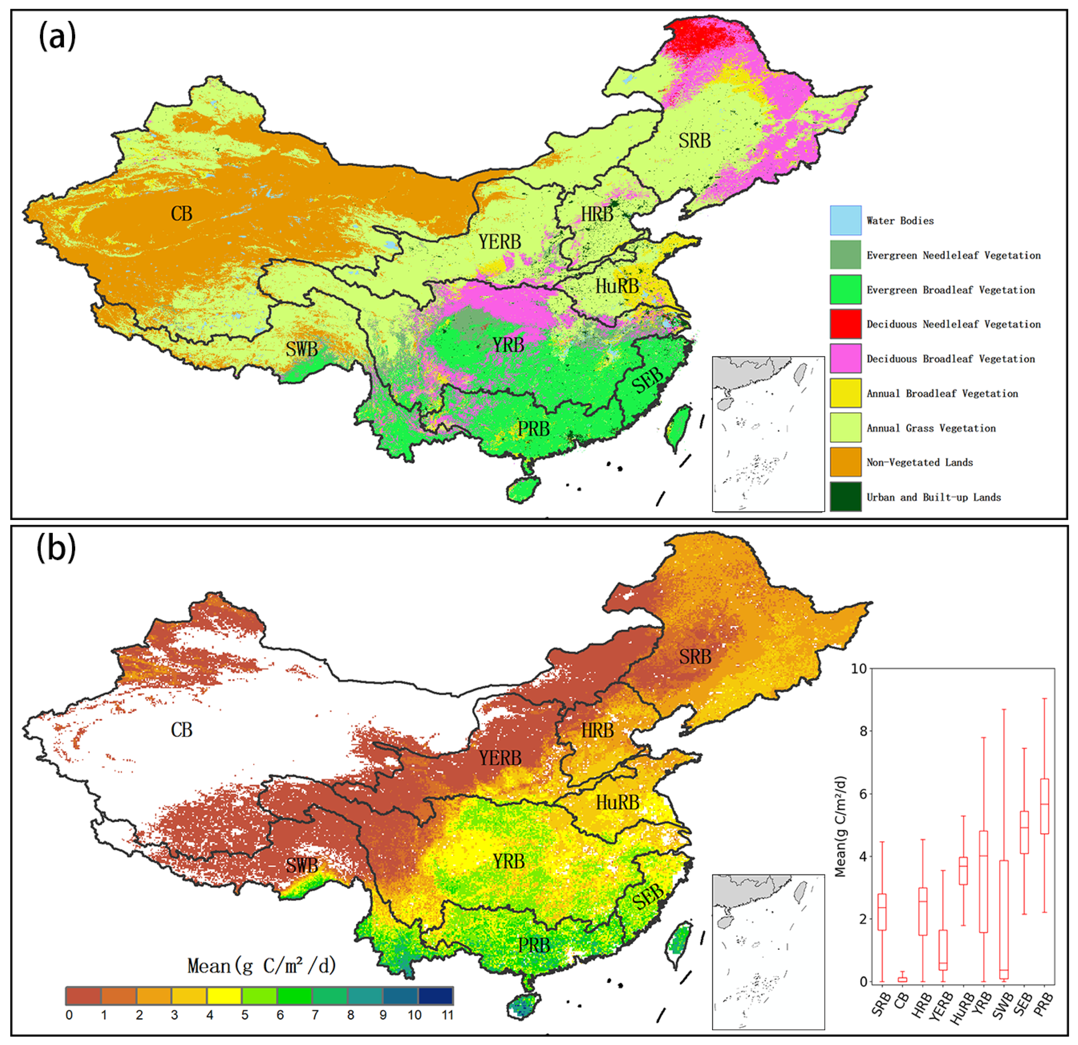
2.1. Study Area
2.2. GPP Product
2.3. Climate and Anthropogenic Variables
2.4. Trend Analysis
2.4.1. Mann–Kendall Test
2.4.2. Sen’s Slope Estimator
2.5. Correlation Analysis
2.6. Autoregressive Integrated Moving Average (ARIMA) Model
2.6.1. Identification
2.6.2. Parameter and Diagnostic Checking
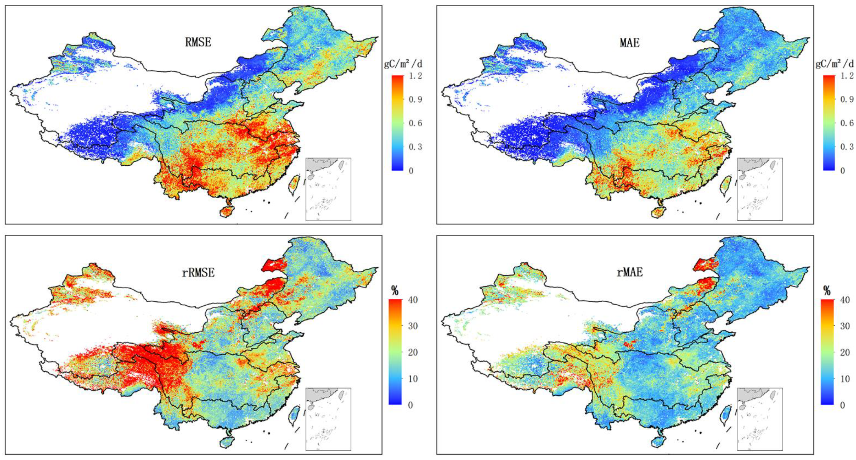
2.6.3. Prediction and Evaluation
2.7. Analysis Framework
3. Result
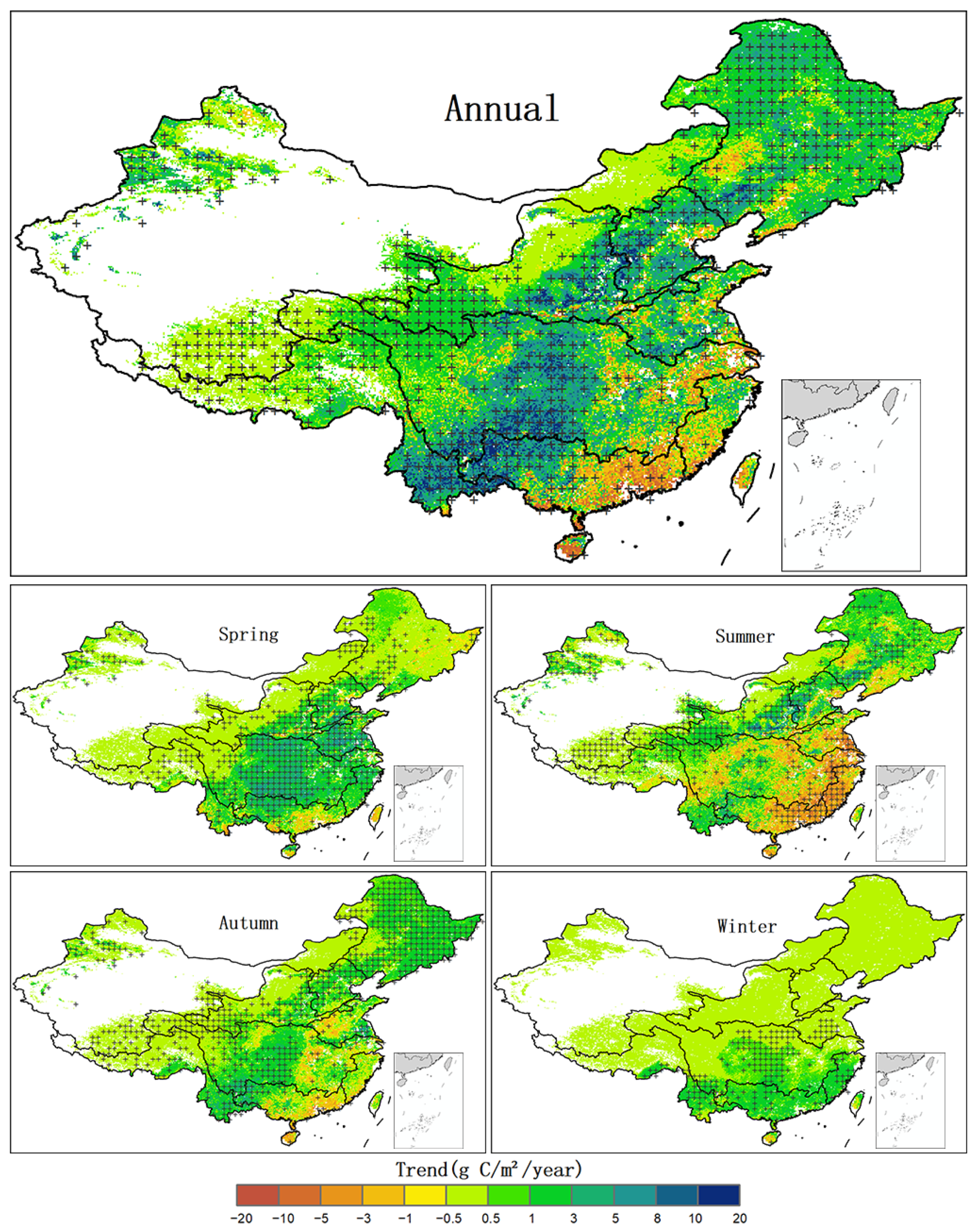
3.1. Annual and Seasonal Trends of GPP Calculated from LUEopt Products
3.2. Attributions of Long-Term Changes in GPP
3.3. Short-Term Prediction of GPP by ARIMA Model
4. Discussion
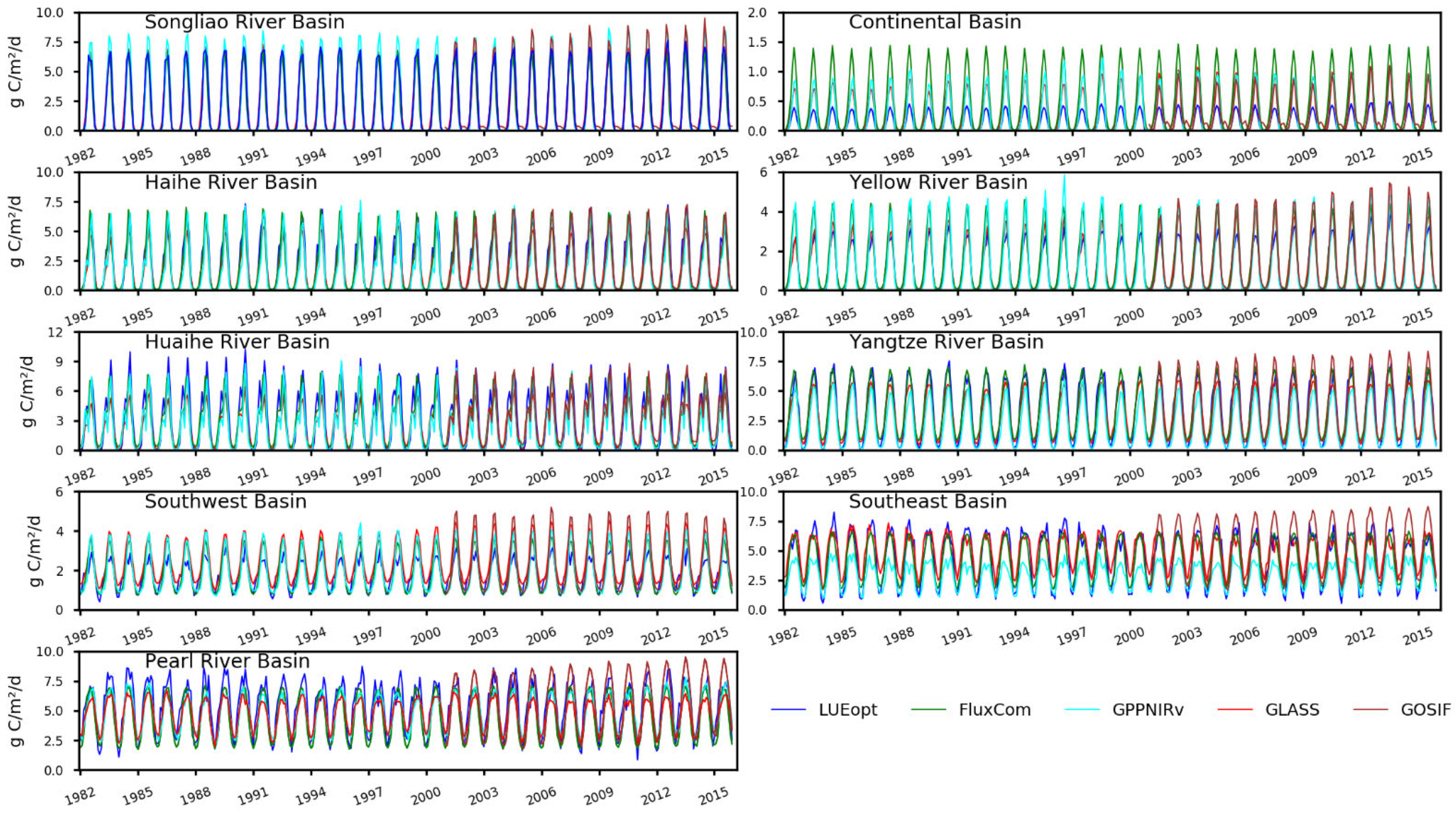
4.1. Comparison of Multi-Source Data
4.2. Implications for Other Biophysical Studies
5. Conclusions
Author Contributions
Funding
Data Availability Statement
Acknowledgments
Conflicts of Interest
Appendix A
References
- Beer, C.; Reichstein, M.; Tomelleri, E.; Ciais, P.; Jung, M.; Carvalhais, N.; Rodenbeck, C.; Arain, M.A.; Baldocchi, D.; Bonan, G.B.; et al. Terrestrial gross carbon dioxide uptake: Global distribution and covariation with climate. Science 2010, 329, 834–838. [Google Scholar] [CrossRef] [PubMed] [Green Version]
- Janssens, I.A.; Freibauer, A.; Ciais, P.; Smith, P.; Nabuurs, G.J.; Folberth, G.; Schlamadinger, B.; Hutjes, R.W.; Ceulemans, R.; Schulze, E.D.; et al. Europe’s terrestrial biosphere absorbs 7 to 12% of European anthropogenic CO2 emissions. Science 2003, 300, 1538–1542. [Google Scholar] [CrossRef] [PubMed] [Green Version]
- Battin, T.J.; Luyssaert, S.; Kaplan, L.A.; Aufdenkampe, A.K.; Richter, A.; Tranvik, L.J. The boundless carbon cycle. Nat. Geosci. 2009, 2, 598–600. [Google Scholar] [CrossRef]
- Gao, Q.; Li, Y.; Wan, Y.; Qin, X.; Jiangcun, W.; Liu, Y. Dynamics of alpine grassland NPP and its response to climate change in Northern Tibet. Clim. Change 2009, 97, 515–528. [Google Scholar] [CrossRef]
- Norby, R.J.; Warren, J.M.; Iversen, C.M.; Medlyn, B.E.; McMurtrie, R.E. CO2 enhancement of forest productivity constrained by limited nitrogen availability. Proc. Natl. Acad. Sci. USA 2010, 107, 19368–19373. [Google Scholar] [CrossRef] [Green Version]
- Schimel, D.; Stephens, B.B.; Fisher, J.B. Effect of increasing CO2 on the terrestrial carbon cycle. Proc. Natl. Acad. Sci. USA 2015, 112, 436–441. [Google Scholar] [CrossRef] [Green Version]
- Cheng, Y.-B.; Zhang, Q.; Lyapustin, A.I.; Wang, Y.; Middleton, E.M. Impacts of light use efficiency and fPAR parameterization on gross primary production modeling. Agric. For. Meteorol. 2014, 189–190, 187–197. [Google Scholar] [CrossRef]
- Zhao, M.; Running, S.W. Drought-induced reduction in global terrestrial net primary production from 2000 through 2009. Science 2010, 329, 940–943. [Google Scholar] [CrossRef] [Green Version]
- Nemani, R.R.; Keeling, C.D.; Hashimoto, H.; Jolly, W.M.; Piper, S.C.; Tucker, C.J.; Myneni, R.B.; Running, S.W. Climate-driven increases in global terrestrial net primary production from 1982 to 1999. Science 2003, 300, 1560–1563. [Google Scholar] [CrossRef] [Green Version]
- Zhang, Y.; Ye, A. Would the obtainable gross primary productivity (GPP) products stand up? A critical assessment of 45 global GPP products. Sci. Total Environ. 2021, 783, 146965. [Google Scholar] [CrossRef]
- Xie, S.; Mo, X.; Hu, S.; Liu, S. Contributions of climate change, elevated atmospheric CO2 and human activities to ET and GPP trends in the Three-North Region of China. Agric. For. Meteorol. 2020, 295, 108183. [Google Scholar] [CrossRef]
- Ge, W.; Han, J.; Zhang, D.; Wang, F. Divergent impacts of droughts on vegetation phenology and productivity in the Yungui Plateau, southwest China. Ecol. Indic. 2021, 127, 107743. [Google Scholar] [CrossRef]
- Song, L.; Li, Y.; Ren, Y.; Wu, X.; Guo, B.; Tang, X.; Shi, W.; Ma, M.; Han, X.; Zhao, L. Divergent vegetation responses to extreme spring and summer droughts in Southwestern China. Agric. For. Meteorol. 2019, 279, 107703. [Google Scholar] [CrossRef]
- Piao, S.; Ciais, P.; Lomas, M.; Beer, C.; Liu, H.; Fang, J.; Friedlingstein, P.; Huang, Y.; Muraoka, H.; Son, Y.; et al. Contribution of climate change and rising CO2 to terrestrial carbon balance in East Asia: A multi-model analysis. Glob. Planet. Chang. 2011, 75, 133–142. [Google Scholar] [CrossRef]
- Liu, K.; Li, X.; Long, X. Trends in groundwater changes driven by precipitation and anthropogenic activities on the southeast side of the Hu Line. Environ. Res. Lett. 2021, 16, 094032. [Google Scholar] [CrossRef]
- Zhu, W.; Pan, Y.; Yang, X.; Song, G. Comprehensive analysis of the impact of climatic changes on Chinese terrestrial net primary productivity. Chin. Sci. Bull. 2007, 52, 3253–3260. [Google Scholar] [CrossRef]
- Khalifa, M.; Elagib, N.A.; Ribbe, L.; Schneider, K. Spatio-temporal variations in climate, primary productivity and efficiency of water and carbon use of the land cover types in Sudan and Ethiopia. Sci. Total Environ. 2018, 624, 790–806. [Google Scholar] [CrossRef]
- Mirza, M. Climate change and extreme weather events: Can developing countries adapt? Clim. Policy 2003, 3, 233–248. [Google Scholar] [CrossRef]
- Ciais, P.; Reichstein, M.; Viovy, N.; Granier, A.; Ogee, J.; Allard, V.; Aubinet, M.; Buchmann, N.; Bernhofer, C.; Carrara, A.; et al. Europe-wide reduction in primary productivity caused by the heat and drought in 2003. Nature 2005, 437, 529–533. [Google Scholar] [CrossRef]
- Zhang, Y.; Zhang, C.; Wang, Z.; Chen, Y.; Gang, C.; An, R.; Li, J. Vegetation dynamics and its driving forces from climate change and human activities in the Three-River Source Region, China from 1982 to 2012. Sci. Total Environ. 2016, 563–564, 210–220. [Google Scholar] [CrossRef]
- Luo, L.; Ma, W.; Zhuang, Y.; Zhang, Y.; Yi, S.; Xu, J.; Long, Y.; Ma, D.; Zhang, Z. The impacts of climate change and human activities on alpine vegetation and permafrost in the Qinghai-Tibet Engineering Corridor. Ecol. Indic. 2018, 93, 24–35. [Google Scholar] [CrossRef]
- Jiang, Y.; Guo, J.; Peng, Q.; Guan, Y.; Zhang, Y.; Zhang, R. The effects of climate factors and human activities on net primary productivity in Xinjiang. Int. J. Biometeorol. 2020, 64, 765–777. [Google Scholar] [CrossRef]
- Woodward, F.I.; Lomas, M.R. Vegetation dynamics--simulating responses to climatic change. Biol. Rev. Camb. Philos. Soc. 2004, 79, 643–670. [Google Scholar] [CrossRef] [PubMed]
- Ardo, J. Comparison between remote sensing and a dynamic vegetation model for estimating terrestrial primary production of Africa. Carbon Balance Manag. 2015, 10, 8. [Google Scholar] [CrossRef] [PubMed] [Green Version]
- Romilly, P. Time series modelling of global mean temperature for managerial decision-making. J. Environ. Manag. 2005, 76, 61–70. [Google Scholar] [CrossRef]
- Yürekli, K.; Simsek, H.; Cemek, B.; Karaman, S. Simulating climatic variables by using stochastic approach. Build. Environ. 2007, 42, 3493–3499. [Google Scholar] [CrossRef]
- Li, X.; Zhang, C.; Zhang, B.; Liu, K. A comparative time series analysis and modeling of aerosols in the contiguous United States and China. Sci. Total Environ. 2019, 690, 799–811. [Google Scholar] [CrossRef]
- Li, X.; Liu, K.; Tian, J. Variability, predictability, and uncertainty in global aerosols inferred from gap-filled satellite observations and an econometric modeling approach. Remote Sens. Environ. 2021, 261, 112501. [Google Scholar] [CrossRef]
- Yuan, C.; Liu, S.; Fang, Z. Comparison of China’s primary energy consumption forecasting by using ARIMA (the autoregressive integrated moving average) model and GM(1,1) model. Energy 2016, 100, 384–390. [Google Scholar] [CrossRef]
- Zhang, L.; Lin, J.; Qiu, R.; Hu, X.; Zhang, H.; Chen, Q.; Tan, H.; Lin, D.; Wang, J. Trend analysis and forecast of PM2.5 in Fuzhou, China using the ARIMA model. Ecol. Indic. 2018, 95, 702–710. [Google Scholar] [CrossRef]
- Valipour, M.; Banihabib, M.E.; Behbahani, S.M.R. Comparison of the ARMA, ARIMA, and the autoregressive artificial neural network models in forecasting the monthly inflow of Dez dam reservoir. J. Hydrol. 2013, 476, 433–441. [Google Scholar] [CrossRef]
- Anav, A.; Friedlingstein, P.; Beer, C.; Ciais, P.; Harper, A.; Jones, C.; Murray-Tortarolo, G.; Papale, D.; Parazoo, N.C.; Peylin, P.; et al. Spatiotemporal patterns of terrestrial gross primary production: A review. Rev. Geophys. 2015, 53, 785–818. [Google Scholar] [CrossRef] [Green Version]
- Wu, M.; Liu, Y.; Xu, Z.; Yan, G.; Ma, M.; Zhou, S.; Qian, Y. Spatio-temporal dynamics of China’s ecological civilization progress after implementing national conservation strategy. J. Clean. Prod. 2021, 285, 124886. [Google Scholar] [CrossRef]
- Jiang, L.; Liu, Y.; Wu, S.; Yang, C. Analyzing ecological environment change and associated driving factors in China based on NDVI time series data. Ecol. Indic. 2021, 129, 107933. [Google Scholar] [CrossRef]
- He, Y.; Wang, M. China’s geographical regionalization in Chinese secondary school curriculum (1902–2012). J. Geogr. Sci. 2013, 23, 370–383. [Google Scholar] [CrossRef]
- Zhang, Z.; Chen, X.; Xu, C.-Y.; Yuan, L.; Yong, B.; Yan, S. Evaluating the non-stationary relationship between precipitation and streamflow in nine major basins of China during the past 50 years. J. Hydrol. 2011, 409, 81–93. [Google Scholar] [CrossRef]
- Madani, N.; Kimball, J.S.; Running, S.W. Improving Global Gross Primary Productivity Estimates by Computing Optimum Light Use Efficiencies Using Flux Tower Data. J. Geophys. Res. Biogeosci. 2017, 122, 2939–2951. [Google Scholar] [CrossRef]
- Madani, N.; Parazoo, N.C.; Kimball, J.S.; Ballantyne, A.P.; Reichle, R.H.; Maneta, M.; Saatchi, S.; Palmer, P.I.; Liu, Z.; Tagesson, T. Recent Amplified Global Gross Primary Productivity due to Temperature Increase Is Offset by Reduced Productivity due to Water Constraints. AGU Adv. 2020, 1, e2020AV000180. [Google Scholar] [CrossRef]
- Wang, S.; Zhang, Y.; Ju, W.; Qiu, B.; Zhang, Z. Tracking the seasonal and inter-annual variations of global gross primary production during last four decades using satellite near-infrared reflectance data. Sci. Total Environ. 2021, 755, 142569. [Google Scholar] [CrossRef]
- Liang, S.; Zhao, X.; Liu, S.; Yuan, W.; Cheng, X.; Xiao, Z.; Zhang, X.; Liu, Q.; Cheng, J.; Tang, H.; et al. A long-term Global LAnd Surface Satellite (GLASS) data-set for environmental studies. Int. J. Digit. Earth 2013, 6, 5–33. [Google Scholar] [CrossRef]
- Tramontana, G.; Jung, M.; Schwalm, C.R.; Ichii, K.; Camps-Valls, G.; Ráduly, B.; Reichstein, M.; Arain, M.A.; Cescatti, A.; Kiely, G.; et al. Predicting carbon dioxide and energy fluxes across global FLUXNET sites with regression algorithms. Biogeosciences 2016, 13, 4291–4313. [Google Scholar] [CrossRef] [Green Version]
- Meroni, M.; Rossini, M.; Guanter, L.; Alonso, L.; Rascher, U.; Colombo, R.; Moreno, J. Remote sensing of solar-induced chlorophyll fluorescence: Review of methods and applications. Remote Sens. Environ. 2009, 113, 2037–2051. [Google Scholar] [CrossRef]
- Li, X.; Xiao, J. A Global, 0.05-Degree Product of Solar-Induced Chlorophyll Fluorescence Derived from OCO-2, MODIS, and Reanalysis Data. Remote Sens. 2019, 11, 517. [Google Scholar] [CrossRef] [Green Version]
- Abatzoglou, J.T.; Dobrowski, S.Z.; Parks, S.A.; Hegewisch, K.C. TerraClimate, a high-resolution global dataset of monthly climate and climatic water balance from 1958–2015. Sci. Data 2018, 5, 170191. [Google Scholar] [CrossRef] [Green Version]
- Claverie, M.; Matthews, J.; Vermote, E.; Justice, C. A 30+ Year AVHRR LAI and FAPAR Climate Data Record: Algorithm Description and Validation. Remote Sens. 2016, 8, 263. [Google Scholar] [CrossRef] [Green Version]
- Qu, Y.; Zhang, C.; Wang, D.; Tian, P.; Bai, W.; Zhang, X.; Zhang, P.; Dai, H.; Wu, Q. Comparison of atmospheric CO2 observed by GOSAT and two ground stations in China. Int. J. Remote Sens. 2013, 34, 3938–3946. [Google Scholar] [CrossRef]
- Gelaro, R.; McCarty, W.; Suárez, M.J.; Todling, R.; Molod, A.; Takacs, L.; Randles, C.A.; Darmenov, A.; Bosilovich, M.G.; Reichle, R.; et al. The Modern-Era Retrospective Analysis for Research and Applications, Version 2 (MERRA-2). J. Clim. 2017, 30, 5419–5454. [Google Scholar] [CrossRef]
- Wu, W.Y.; Lo, M.H.; Wada, Y.; Famiglietti, J.S.; Reager, J.T.; Yeh, P.J.; Ducharne, A.; Yang, Z.L. Divergent effects of climate change on future groundwater availability in key mid-latitude aquifers. Nat. Commun. 2020, 11, 3710. [Google Scholar] [CrossRef]
- Hamed, K.H. Exact distribution of the Mann–Kendall trend test statistic for persistent data. J. Hydrol. 2009, 365, 86–94. [Google Scholar] [CrossRef]
- Gocic, M.; Trajkovic, S. Analysis of changes in meteorological variables using Mann-Kendall and Sen’s slope estimator statistical tests in Serbia. Glob. Planet. Chang. 2013, 100, 172–182. [Google Scholar] [CrossRef]
- Zscheischler, J.; Michalak, A.M.; Schwalm, C.; Mahecha, M.D.; Huntzinger, D.N.; Reichstein, M.; Berthier, G.; Ciais, P.; Cook, R.B.; El-Masri, B.; et al. Impact of large-scale climate extremes on biospheric carbon fluxes: An intercomparison based on MsTMIP data. Glob. Biogeochem. Cycles 2014, 28, 585–600. [Google Scholar] [CrossRef]
- Zhang, X.; Liu, K.; Wang, S.; Wu, T.; Li, X.; Wang, J.; Wang, D.; Zhu, H.; Tan, C.; Ji, Y. Spatiotemporal evolution of ecological vulnerability in the Yellow River Basin under ecological restoration initiatives. Ecol. Indic. 2022, 135, 108586. [Google Scholar] [CrossRef]
- Zhang, X.; Liu, K.; Li, X.; Wang, S.; Wang, J. Vulnerability assessment and its driving forces in terms of NDVI and GPP over the Loess Plateau, China. Phys. Chem. Earth Parts A/B/C 2022, 125, 103106. [Google Scholar] [CrossRef]
- Wang, X.; Lu, C.; Fang, J.; Shen, Y. Implications for development of grain-for-green policy based on cropland suitability evaluation in desertification-affected north China. Land Use Policy 2007, 24, 417–424. [Google Scholar] [CrossRef]
- Liu, J.; Xu, X.; Shao, Q. Grassland degradation in the “Three-River Headwaters” region, Qinghai Province. J. Geogr. Sci. 2008, 18, 259–273. [Google Scholar] [CrossRef]
- Cui, Y. Preliminary estimation of the realistic optimum temperature for vegetation growth in China. Environ. Manag. 2013, 52, 151–162. [Google Scholar] [CrossRef]
- Guha, A.; Han, J.; Cummings, C.; McLennan, D.A.; Warren, J.M. Differential ecophysiological responses and resilience to heat wave events in four co-occurring temperate tree species. Environ. Res. Lett. 2018, 13, 065008. [Google Scholar] [CrossRef]
- Shi, H.; Chen, J. Characteristics of climate change and its relationship with land use/cover change in Yunnan Province, China. Int. J. Climatol. 2018, 38, 2520–2537. [Google Scholar] [CrossRef]
- Li, Z.; Chen, Y.; Wang, Y.; Fang, G. Dynamic changes in terrestrial net primary production and their effects on evapotranspiration. Hydrol. Earth Syst. Sci. 2016, 20, 2169–2178. [Google Scholar] [CrossRef] [Green Version]
- Liu, Y.; Xiao, J.; Ju, W.; Zhou, Y.; Wang, S.; Wu, X. Water use efficiency of China’s terrestrial ecosystems and responses to drought. Sci. Rep. 2015, 5, 13799. [Google Scholar] [CrossRef]
- Peng, C.; Zhou, X.; Zhao, S.; Wang, X.; Zhu, B.; Piao, S.; Fang, J. Quantifying the response of forest carbon balance to future climate change in Northeastern China: Model validation and prediction. Glob. Planet. Chang. 2009, 66, 179–194. [Google Scholar] [CrossRef]
- Sirvydas, A.; Kučinskas, V.; Kerpauskas, P.; Nadzeikienė, J.; Kusta, A. Solar Radiation Energy Pulsations in a Plant Leaf. J. Environ. Eng. Landsc. Manag. 2010, 18, 188–195. [Google Scholar] [CrossRef]
- Durand, M.; Murchie, E.H.; Lindfors, A.V.; Urban, O.; Aphalo, P.J.; Robson, T.M. Diffuse solar radiation and canopy photosynthesis in a changing environment. Agric. For. Meteorol. 2021, 311, 108684. [Google Scholar] [CrossRef]
- Feng, X.; Fu, B.; Piao, S.; Wang, S.; Ciais, P.; Zeng, Z.; Lü, Y.; Zeng, Y.; Li, Y.; Jiang, X.; et al. Revegetation in China’s Loess Plateau is approaching sustainable water resource limits. Nat. Clim. Chang. 2016, 6, 1019–1022. [Google Scholar] [CrossRef]
- Wang, S.; Li, G.; Fang, C. Urbanization, economic growth, energy consumption, and CO2 emissions: Empirical evidence from countries with different income levels. Renew. Sustain. Energy Rev. 2018, 81, 2144–2159. [Google Scholar] [CrossRef]
- Devaraju, N.; Bala, G.; Caldeira, K.; Nemani, R. A model based investigation of the relative importance of CO2-fertilization, climate warming, nitrogen deposition and land use change on the global terrestrial carbon uptake in the historical period. Clim. Dyn. 2015, 47, 173–190. [Google Scholar] [CrossRef]
- He, Q.; Zhang, M.; Huang, B. Spatio-temporal variation and impact factors analysis of satellite-based aerosol optical depth over China from 2002 to 2015. Atmos. Environ. 2016, 129, 79–90. [Google Scholar] [CrossRef]
- Levy, R.C.; Mattoo, S.; Munchak, L.A.; Remer, L.A.; Sayer, A.M.; Patadia, F.; Hsu, N.C. The Collection 6 MODIS aerosol products over land and ocean. Atmos. Meas. Tech. 2013, 6, 2989–3034. [Google Scholar] [CrossRef] [Green Version]
- Li, X.; Zhang, C.; Li, W.; Liu, K. Evaluating the Use of DMSP/OLS Nighttime Light Imagery in Predicting PM2.5 Concentrations in the Northeastern United States. Remote Sens. 2017, 9, 620. [Google Scholar] [CrossRef] [Green Version]
- Li, X.; Liang, H.; Cheng, W. Spatio-Temporal Variation in AOD and Correlation Analysis with PAR and NPP in China from 2001 to 2017. Remote Sens. 2020, 12, 976. [Google Scholar] [CrossRef] [Green Version]
- Li, X.; Seth, A.; Zhang, C.; Feng, R.; Long, X.; Li, W.; Liu, K. Evaluation of WRF-CMAQ simulated climatological mean and extremes of fine particulate matter of the United States and its correlation with climate extremes. Atmos. Environ. 2020, 222, 117181. [Google Scholar] [CrossRef]
- Li, X.; Zhang, C.; Li, W.; Anyah, R.O.; Tian, J. Exploring the trend, prediction and driving forces of aerosols using satellite and ground data, and implications for climate change mitigation. J. Clean. Prod. 2019, 223, 238–251. [Google Scholar] [CrossRef]
- Soni, K.; Parmar, K.S.; Kapoor, S.; Kumar, N. Statistical variability comparison in MODIS and AERONET derived aerosol optical depth over Indo-Gangetic Plains using time series modeling. Sci. Total Environ. 2016, 553, 258–265. [Google Scholar] [CrossRef] [PubMed]
- Gampe, D.; Zscheischler, J.; Reichstein, M.; O’Sullivan, M.; Smith, W.K.; Sitch, S.; Buermann, W. Increasing impact of warm droughts on northern ecosystem productivity over recent decades. Nat. Clim. Chang. 2021, 11, 772–779. [Google Scholar] [CrossRef]


| ID | Variables | Source | Time Period | Temporal Resolution | Spatial Resolution | Units |
|---|---|---|---|---|---|---|
| 1 | GPP | Oak Ridge National Laboratory | 1982–2016 | Monthly | 8 × 8 km | gC/m2/day |
| 2 | GPP | National Tibetan Plateau Data Center | 1982–2016 | Monthly | 0.05 × 0.05° | gC/m2/day |
| 3 | GPP | National Earth System Science Data Center | 1982–2016 | 8 days | 0.05 × 0.05° | gC/m2/8 days |
| 4 | GPP | FluxCom | 1982–2016 | Monthly | 0.5 × 0.5° | gC/m2/day |
| 5 | GPP | Global Ecology Group | 2001–2016 | 8 days | 0.05 × 0.05° | gC/m2/month |
| 6 | Air temperature | Terraclimate | 1982–2015 | Monthly | 4 × 4 km | Degree (°)/month |
| 7 | Precipitation | Terraclimate | 1982–2015 | Monthly | 4 × 4 km | mm/month |
| 8 | SRAD | Terraclimate | 1980–2015 | Monthly | 4 × 4 km | W/m2/month |
| 9 | LAI | AVHRR | 1982–2015 | 8 days | 0.05 × 0.05° | m2/m2 |
| 10 | CO2 | GOSAT | 2010–2015 | Monthly | 2.5 × 2.5° | ppm/month |
| 11 | AOD | MERRA-2 | 1982–2015 | Monthly | 0.625 × 0.50° | \ |
| Region | Air Temperature | SRAD | Precipitation | LAI | AOD | CO2 | ||||||
|---|---|---|---|---|---|---|---|---|---|---|---|---|
| Mean | STD | Mean | STD | Mean | STD | Mean | STD | Mean | STD | Mean | STD | |
| SRB | 0.145 | 0.212 | 0.065 | 0.305 | −0.03 | 0.343 | 0.4 | 0.217 | −0.126 | 0.254 | 0.229 | 0.479 |
| CB | 0.265 | 0.266 | −0.327 | 0.208 | 0.263 | 0.222 | 0.307 | 0.249 | −0.132 | 0.198 | 0.013 | 0.484 |
| HRB | 0.206 | 0.155 | −0.241 | 0.135 | 0.372 | 0.172 | 0.501 | 0.198 | 0.101 | 0.186 | 0.204 | 0.385 |
| YERB | 0.252 | 0.165 | −0.201 | 0.208 | 0.224 | 0.189 | 0.427 | 0.239 | 0.008 | 0.211 | 0.268 | 0.431 |
| HuRB | 0.225 | 0.164 | −0.029 | 0.218 | 0.143 | 0.215 | 0.364 | 0.187 | 0.052 | 0.216 | 0.251 | 0.34 |
| YRB | 0.291 | 0.214 | 0.178 | 0.269 | −0.03 | 0.228 | 0.271 | 0.225 | 0.021 | 0.243 | 0.21 | 0.483 |
| SWB | 0.359 | 0.194 | −0.003 | 0.24 | −0.038 | 0.22 | 0.228 | 0.214 | −0.204 | 0.155 | −0.101 | 0.438 |
| SEB | −0.002 | 0.196 | 0.231 | 0.168 | −0.194 | 0.159 | 0.057 | 0.195 | −0.072 | 0.212 | 0.174 | 0.359 |
| PRB | 0.039 | 0.208 | 0.134 | 0.146 | −0.186 | 0.16 | 0.152 | 0.272 | −0.025 | 0.311 | 0.176 | 0.432 |
| China | 0.225 | 0.229 | −0.012 | 0.307 | 0.053 | 0.29 | 0.318 | 0.248 | −0.056 | 0.246 | 0.16 | 0.47 |
Publisher’s Note: MDPI stays neutral with regard to jurisdictional claims in published maps and institutional affiliations. |
© 2022 by the authors. Licensee MDPI, Basel, Switzerland. This article is an open access article distributed under the terms and conditions of the Creative Commons Attribution (CC BY) license (https://creativecommons.org/licenses/by/4.0/).
Share and Cite
Bo, Y.; Li, X.; Liu, K.; Wang, S.; Zhang, H.; Gao, X.; Zhang, X. Three Decades of Gross Primary Production (GPP) in China: Variations, Trends, Attributions, and Prediction Inferred from Multiple Datasets and Time Series Modeling. Remote Sens. 2022, 14, 2564. https://doi.org/10.3390/rs14112564
Bo Y, Li X, Liu K, Wang S, Zhang H, Gao X, Zhang X. Three Decades of Gross Primary Production (GPP) in China: Variations, Trends, Attributions, and Prediction Inferred from Multiple Datasets and Time Series Modeling. Remote Sensing. 2022; 14(11):2564. https://doi.org/10.3390/rs14112564
Chicago/Turabian StyleBo, Yong, Xueke Li, Kai Liu, Shudong Wang, Hongyan Zhang, Xiaojie Gao, and Xiaoyuan Zhang. 2022. "Three Decades of Gross Primary Production (GPP) in China: Variations, Trends, Attributions, and Prediction Inferred from Multiple Datasets and Time Series Modeling" Remote Sensing 14, no. 11: 2564. https://doi.org/10.3390/rs14112564
APA StyleBo, Y., Li, X., Liu, K., Wang, S., Zhang, H., Gao, X., & Zhang, X. (2022). Three Decades of Gross Primary Production (GPP) in China: Variations, Trends, Attributions, and Prediction Inferred from Multiple Datasets and Time Series Modeling. Remote Sensing, 14(11), 2564. https://doi.org/10.3390/rs14112564