
Incorporating a Hyperspectral Direct-Diffuse Pyranometer in an Above-Water Reflectance Algorithm


Abstract
:1. Introduction
2. Field Data and Sensors
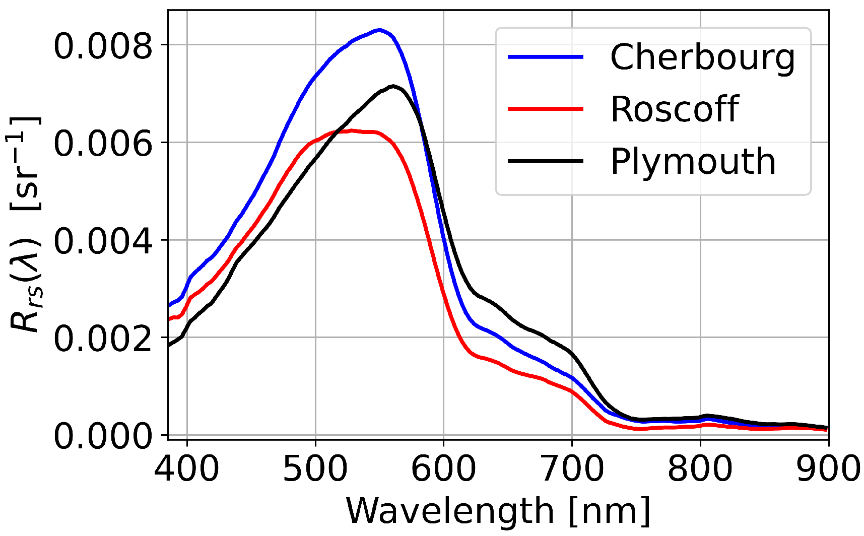
2.1. Field Data
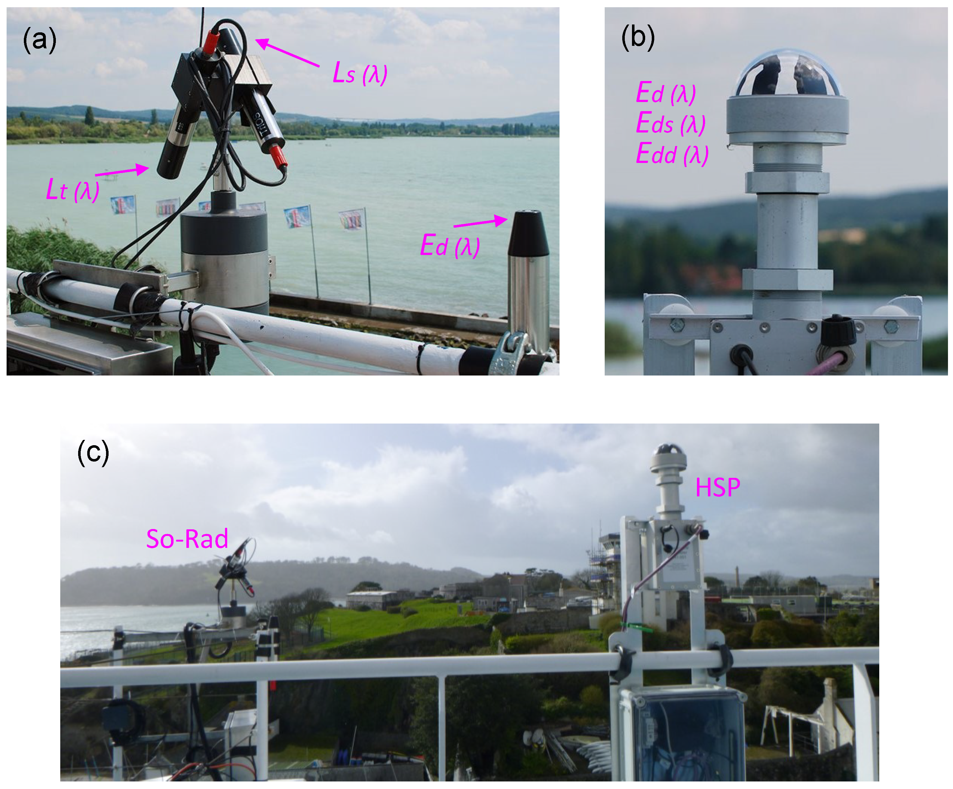
2.2. The Solar-Tracking Radiometry Platform (So-Rad)
2.3. The Hyperspectral Pyranometer (HSP)
2.4. Data Combination Prior to Processing
3. Reflectance Processing
3.1. Overview of Algorithm Variants
- (1)
- (2)
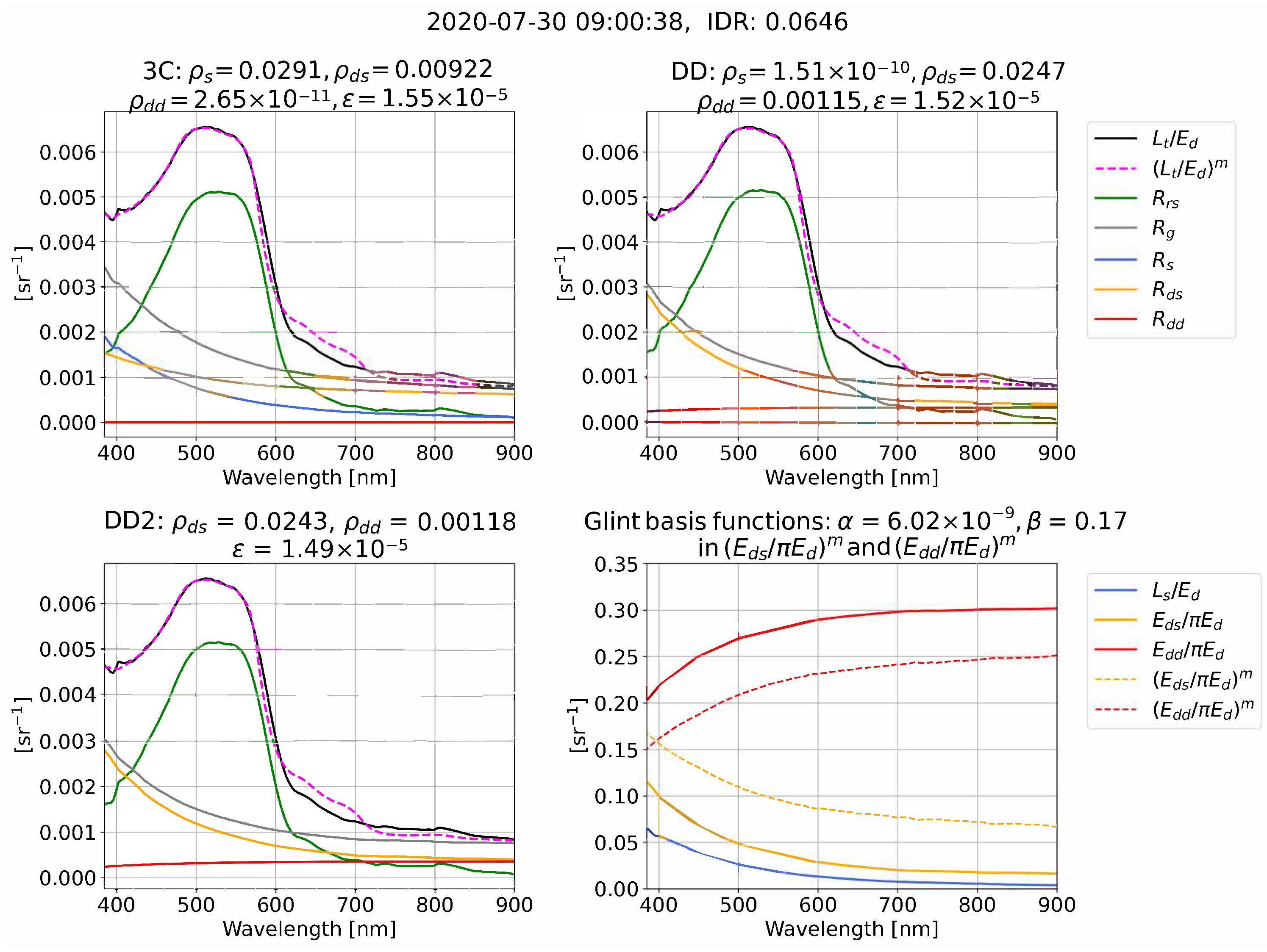
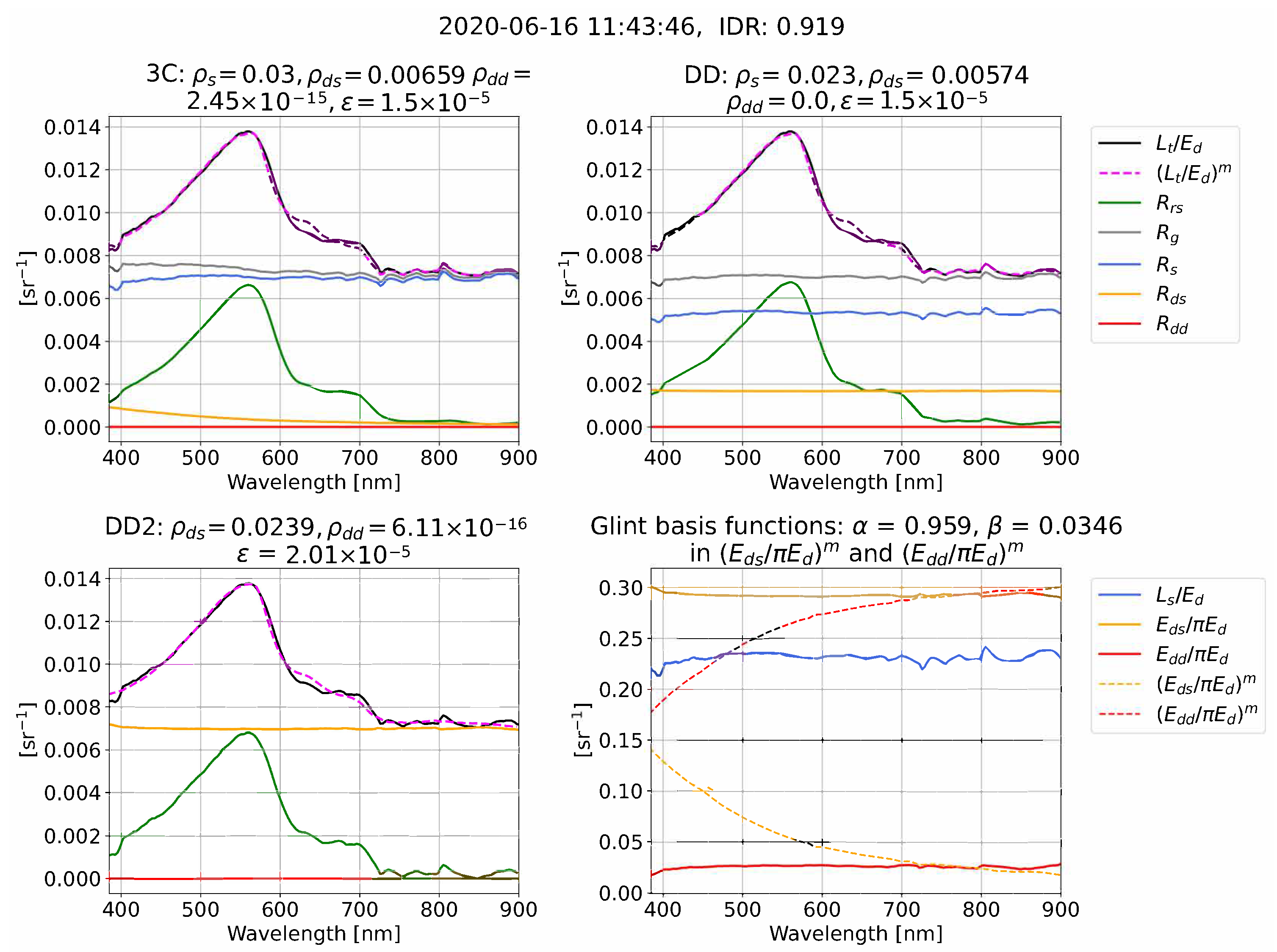
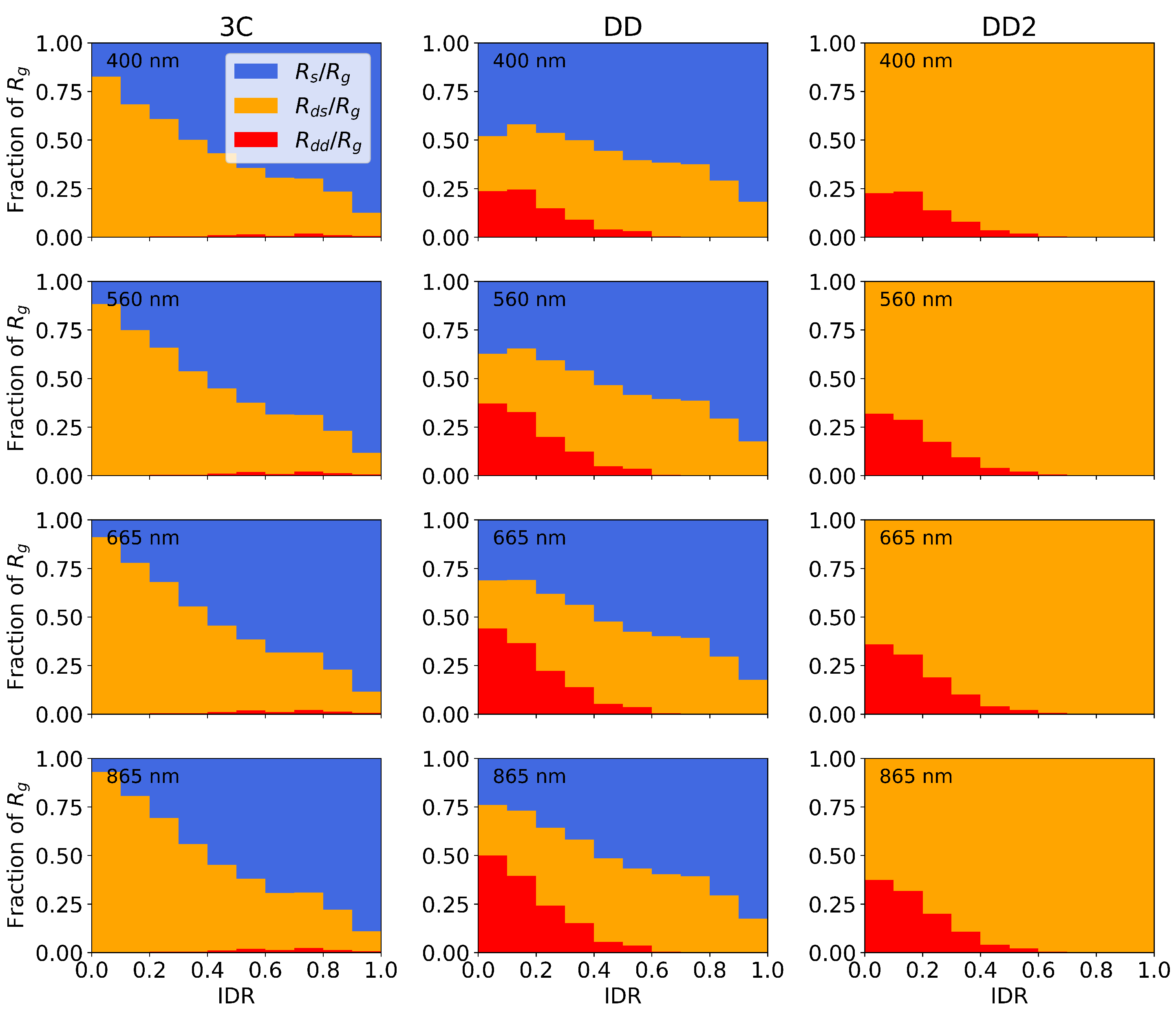
- DD (direct-diffuse). This is 3C-like processing using the water model but not the atmospheric model, and extending the observed spectral ratios to be , , , and .
- (3)
- DD2 (direct-diffuse with two sensors). This is 3C-like processing using the water but not the atmospheric model and using , , and as observed spectral ratios (i.e., removing the sensor). This corresponds to measurements from a hypothetical two-sensor system ( spectroradiometer and HSP pyranometer for , , and ).
3.2. Water and Atmospheric Models Used in Spectral Optimization
3.3. Spectral Optimization Procedure
3.4. Examples of Reflectance Processing and Glint Corrections
3.5. Quality Control
3.6. Computation of Variability
4. Results
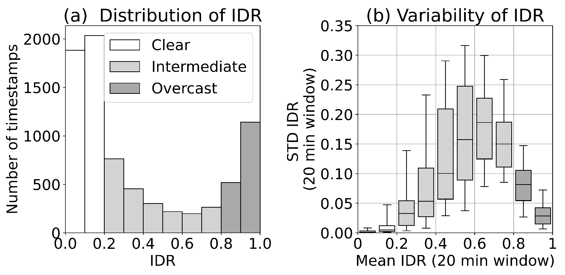
4.1. Atmospheric Optical State
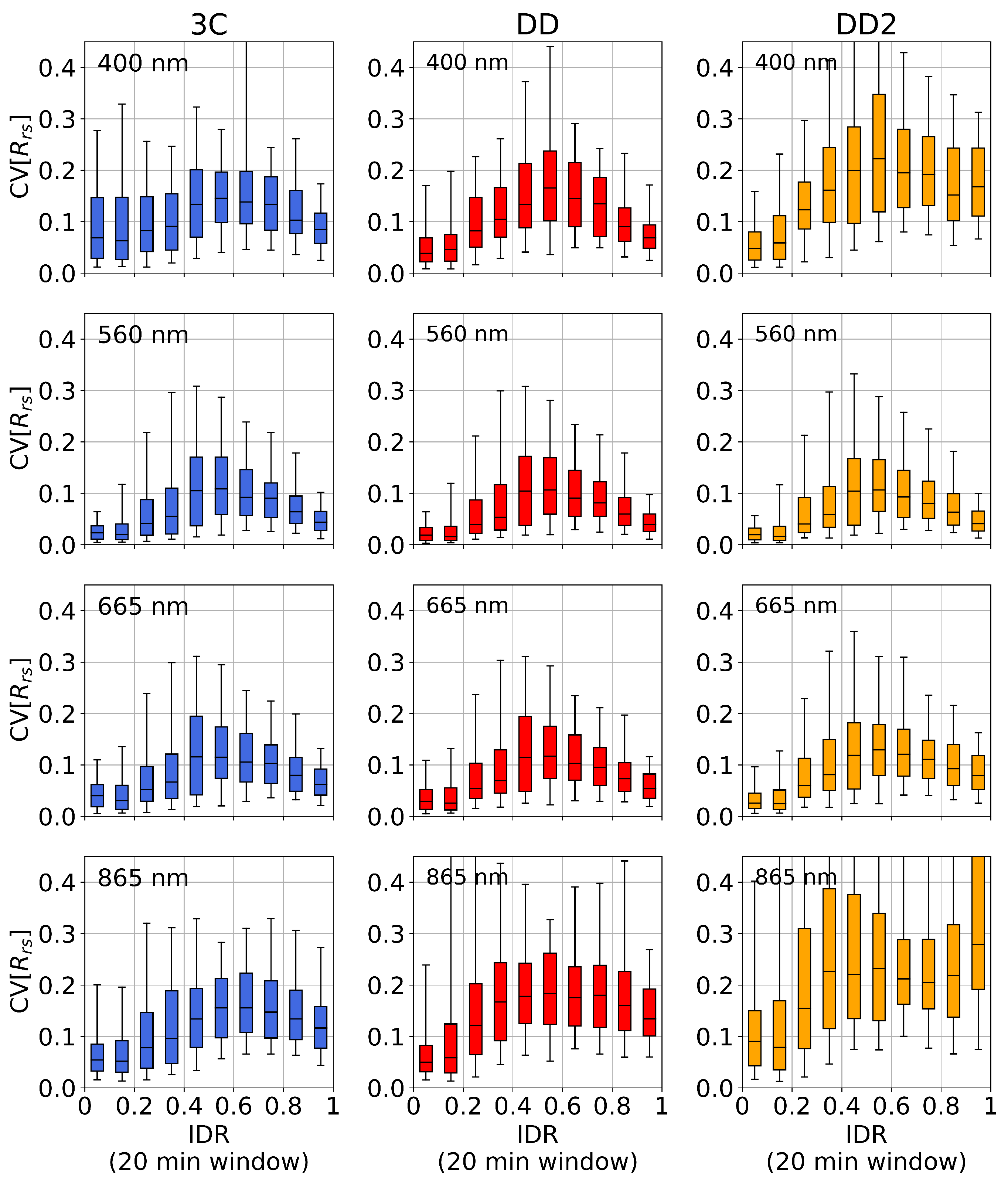
4.2. Atmospheric Dependence of Variability
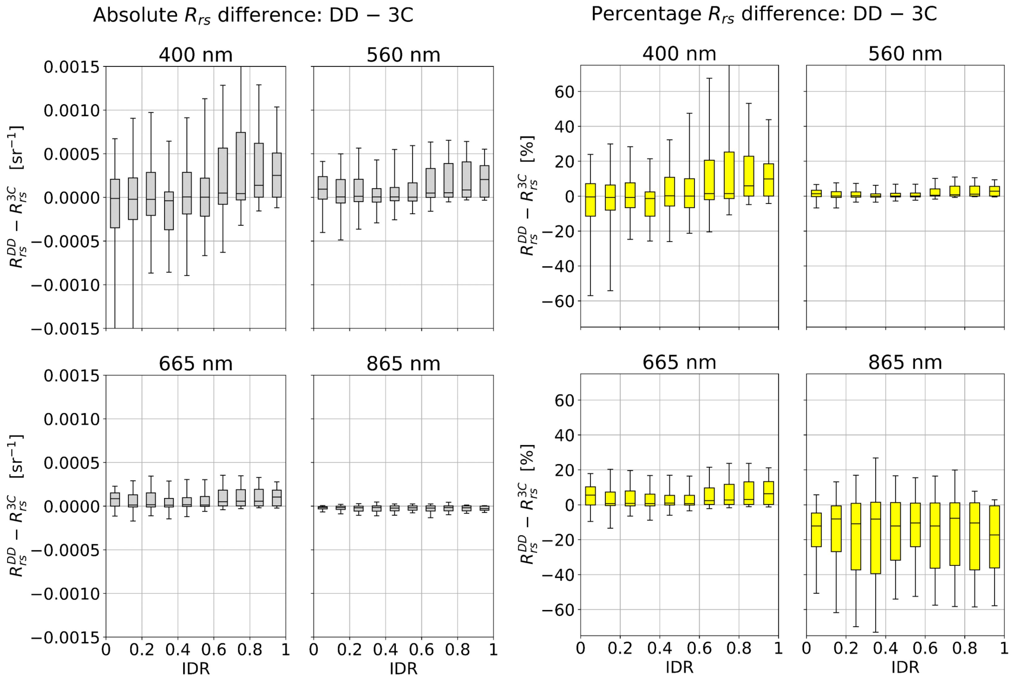
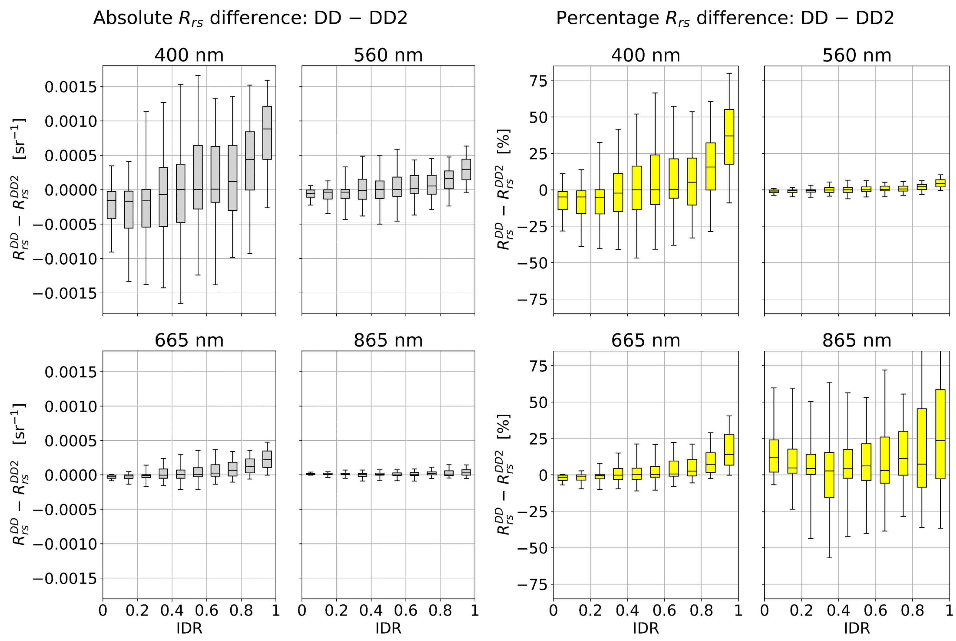
4.3. Atmospheric Dependence of Differences
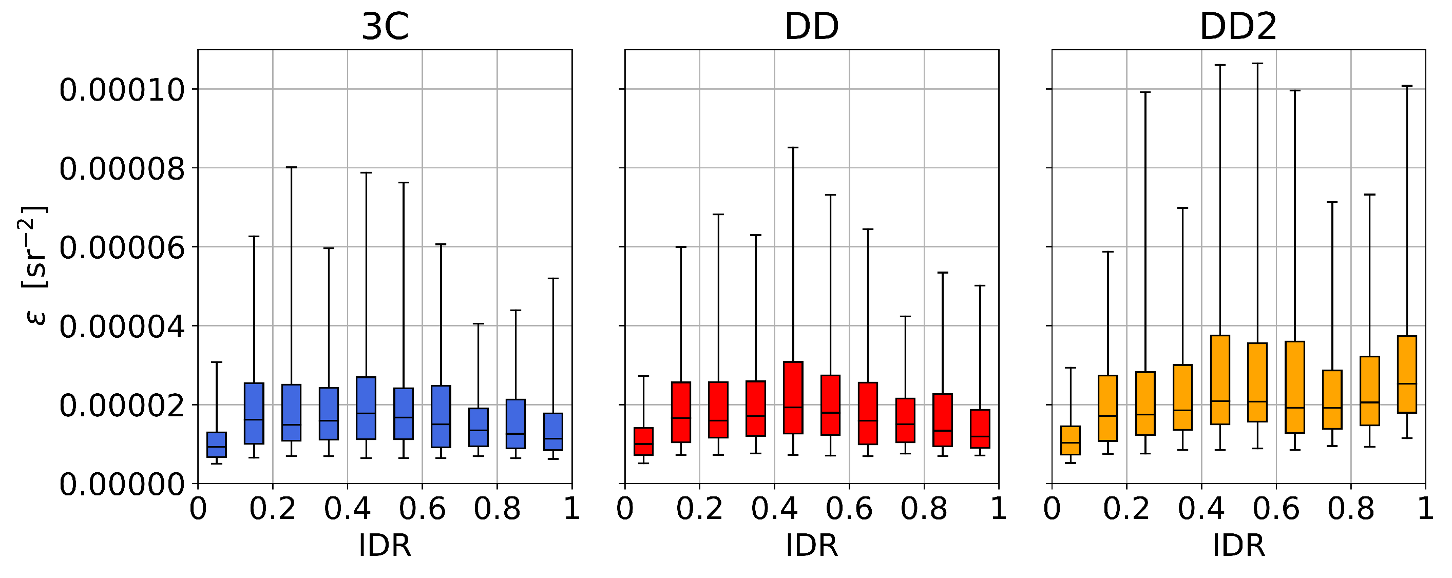
4.4. Atmospheric Dependence of Glint Corrections and Algorithm Residuals
5. Discussion
6. Summary
Author Contributions
Funding
Data Availability Statement
Acknowledgments
Conflicts of Interest
References
- Ruddick, K.G.; Voss, K.; Boss, E.; Castagna, A.; Frouin, R.; Gilerson, A.; Hieronymi, M.; Johnson, B.C.; Kuusk, J.; Lee, Z.; et al. A Review of Protocols for Fiducial Reference Measurements of Water-Leaving Radiance for Validation of Satellite Remote-Sensing Data over Water. Remote Sens. 2019, 11, 2198. [Google Scholar] [CrossRef] [Green Version]
- Zibordi, G.; Voss, K.J.; Johnson, B.C.; Mueller, J.L. Protocols for Satellite Ocean Colour Data Validation: In Situ Optical Radiometry. In IOCCG Ocean Optics & Biogeochemistry Protocols for Satellite Ocean Colour Sensor Validation; IOCCG: Dartmouth, NS, Canada, 2019; Volume 3. [Google Scholar]
- Groom, S.; Sathyendranath, S.; Ban, Y.; Bernard, S.; Brewin, R.; Brotas, V.; Brockmann, C.; Chauhan, P.; Choi, J.k.; Chuprin, A.; et al. Satellite Ocean Colour: Current Status and Future Perspective. Front. Mar. Sci. 2019, 6, 485. [Google Scholar] [CrossRef] [Green Version]
- Zibordi, G.; Ruddick, K.; Ansko, I.; Moore, G.; Kratzer, S.; Icely, J.; Reinart, A. In situ determination of the remote sensing reflectance: An inter-comparison. Ocean Sci. 2012, 8, 567–586. [Google Scholar] [CrossRef] [Green Version]
- Lee, Z.; Pahlevan, N.; Ahn, Y.H.; Greb, S.; O’Donnell, D. Robust approach to directly measuring water-leaving radiance in the field. Appl. Opt. 2013, 52, 1693–1701. [Google Scholar] [CrossRef] [PubMed]
- Mobley, C.D. Estimation of the remote-sensing reflectance from above-surface measurements. Appl. Opt. 1999, 38, 7442–7455. [Google Scholar] [CrossRef] [PubMed]
- Simis, S.G.H.; Olsson, J. Unattended processing of shipborne hyperspectral reflectance measurements. Remote Sens. Environ. 2013, 135, 202–212. [Google Scholar] [CrossRef] [Green Version]
- Kutser, T.; Vahtmäe, E.; Paavel, B.; Kauer, T. Removing glint effects from field radiometry data measured in optically complex coastal and inland waters. Remote Sens. Environ. 2013, 133, 85–89. [Google Scholar] [CrossRef]
- Bernardo, N.; Alcântara, E.; Watanabe, F.; Rodrigues, T.; Carmo, A.; Gomes, A.; Andrade, C. Glint Removal Assessment to Estimate the Remote Sensing Reflectance in Inland Waters with Widely Differing Optical Properties. Remote Sens. 2018, 10, 1655. [Google Scholar] [CrossRef] [Green Version]
- Lee, Z.; Ahn, Y.H.; Mobley, C.; Arnone, R. Removal of surface-reflected light for the measurement of remote-sensing reflectance from an above-surface platform. Opt. Express 2010, 18, 26313–26324. [Google Scholar] [CrossRef]
- Groetsch, P.M.M.; Foster, R.; Gilerson, A. Exploring the limits for sky and sun glint correction of hyperspectral above-surface reflectance observations. Appl. Opt. 2020, 59, 2942–2954. [Google Scholar] [CrossRef]
- Ruddick, K.G.; De Cauwer, V.; Park, Y.J.; Moore, G. Seaborne measurements of near infrared water-leaving reflectance: The similarity spectrum for turbid waters. Limnol. Oceanogr. 2006, 51, 1167–1179. [Google Scholar] [CrossRef] [Green Version]
- Mobley, C.D. Polarized reflectance and transmittance properties of windblown sea surfaces. Appl. Opt. 2015, 54, 4828–4849. [Google Scholar] [CrossRef] [PubMed]
- Cox, C.; Munk, W. Measurement of the Roughness of the Sea Surface from Photographs of the Sun’s Glitter. J. Opt. Soc. Am. 1954, 44, 838–850. [Google Scholar] [CrossRef]
- Groetsch, P.M.M.; Gege, P.; Simis, S.G.H.; Eleveld, M.A.; Peters, S.W.M. Validation of a spectral correction procedure for sun and sky reflections in above-water reflectance measurements. Opt. Express 2017, 25, A742–A761. [Google Scholar] [CrossRef] [PubMed] [Green Version]
- Jiang, D.; Matsushita, B.; Yang, W. A simple and effective method for removing residual reflected skylight in above-water remote sensing reflectance measurements. ISPRS J. Photogramm. Remote Sens. 2020, 165, 16–27. [Google Scholar] [CrossRef]
- Gordon, H.R.; Wang, M. Retrieval of water-leaving radiance and aerosol optical thickness over the oceans with SeaWiFS: A preliminary algorithm. Appl. Opt. 1994, 33, 443–452. [Google Scholar] [CrossRef]
- Groetsch, P.M.M.; Gege, P.; Simis, S.G.H.; Eleveld, M.A.; Peters, S.W.M. Variability of adjacency effects in sky reflectance measurements. Opt. Lett. 2017, 42, 3359–3362. [Google Scholar] [CrossRef] [Green Version]
- Pitarch, J.; Talone, M.; Zibordi, G.; Groetsch, P. Determination of the remote-sensing reflectance from above-water measurements with the 3C model: A further assessment. Opt. Express 2020, 28, 15885–15906. [Google Scholar] [CrossRef]
- Gregg, W.W.; Carder, K.L. A simple spectral solar irradiance model for cloudless maritime atmospheres. Limnol. Oceanogr. 1990, 35, 1657–1675. [Google Scholar] [CrossRef]
- Albert, A.; Mobley, C. An analytical model for subsurface irradiance and remote sensing reflectance in deep and shallow case-2 waters. Opt. Express 2003, 11, 2873–2890. [Google Scholar] [CrossRef]
- Gege, P. Analytic model for the direct and diffuse components of downwelling spectral irradiance in water. Appl. Opt. 2012, 51, 1407–1419. [Google Scholar] [CrossRef] [PubMed] [Green Version]
- Wright, A.; Simis, S.G.H. Construction of the Solar-Tracking Radiometry Platform (So-Rad). Zenodo. 2021. Available online: https://zenodo.org/record/4485805#.Yofi4qjMJPY (accessed on 10 May 2022).
- Wood, J.; Smyth, T.J.; Estellés, V. Autonomous marine hyperspectral radiometers for determining solar irradiances and aerosol optical properties. Atmos. Meas. Tech. 2017, 10, 1723–1737. [Google Scholar] [CrossRef] [Green Version]
- Norgren, M.S.; Wood, J.; Schmidt, K.S.; van Diedenhoven, B.; Stamnes, S.A.; Ziemba, L.D.; Crosbie, E.C.; Shook, M.A.; Kittelman, A.S.; LeBlanc, S.E.; et al. Above-aircraft cirrus cloud and aerosol optical depth from hyperspectral irradiances measured by a total-diffuse radiometer. Atmos. Meas. Tech. 2022, 15, 1373–1394. [Google Scholar] [CrossRef]
- Warren, M.A.; Simis, S.G.H.; Martinez-Vicente, V.; Poser, K.; Bresciani, M.; Alikas, K.; Spyrakos, E.; Giardino, C.; Ansper, A. Assessment of atmospheric correction algorithms for the Sentinel-2A MultiSpectral Imager over coastal and inland waters. Remote Sens. Environ. 2019, 225, 267–289. [Google Scholar] [CrossRef]
- Buiteveld, H.; Hakvoort, J.H.M.; Donze, M. Optical properties of pure water. In Ocean Optics XII; Jaffe, J.S., Ed.; International Society for Optics and Photonics, SPIE: Bellingham, WA, USA, 1994; Volume 2258, pp. 174–183. [Google Scholar] [CrossRef]
- Gege, P. Characterization of the phytoplankton in Lake Constance for classification by remote sensing. Arch. Hydrobiol. Spec. Issues Advanc. Limnol. 1998, 0, 179–193. [Google Scholar]
- Park, Y.J.; Ruddick, K. Model of remote-sensing reflectance including bidirectional effects for case 1 and case 2 waters. Appl. Opt. 2005, 44, 1236–1249. [Google Scholar] [CrossRef]
- Byrd, R.H.; Lu, P.; Nocedal, J.; Zhu, C. A Limited Memory Algorithm for Bound Constrained Optimization. SIAM J. Sci. Comput. 1995, 16, 1190–1208. [Google Scholar] [CrossRef]
- Simis, S.; Jackson, T.; Jordan, T.; Peters, S.; Ghebrehiwot, S. Monda: Monocle Data Analysis Python Package: 2022. Available online: https://github.com/monocle-h2020/MONDA (accessed on 10 May 2022).
- Concha, J.A.; Bracaglia, M.; Brando, V.E. Assessing the influence of different validation protocols on Ocean Colour match-up analyses. Remote Sens. Environ. 2021, 259, 112415. [Google Scholar] [CrossRef]
- Ruddick, K.G.; Voss, K.; Banks, A.C.; Boss, E.; Castagna, A.; Frouin, R.; Hieronymi, M.; Jamet, C.; Johnson, B.C.; Kuusk, J.; et al. A Review of Protocols for Fiducial Reference Measurements of Downwelling Irradiance for the Validation of Satellite Remote Sensing Data over Water. Remote Sens. 2019, 11, 1742. [Google Scholar] [CrossRef] [Green Version]
- Twardowski, M.S.; Boss, E.; Sullivan, J.M.; Donaghay, P.L. Modeling the spectral shape of absorption by chromophoric dissolved organic matter. Mar. Chem. 2004, 89, 69–88. [Google Scholar] [CrossRef]


| Parameter Group | Parameter Name | Symbol and Units | IC [min, max] |
|---|---|---|---|
| Water properties | Chlorophyll-a concentration | [mg m] | 5 [0.01, 100] |
| CDOM absorption at 440 nm | [nm] | 0.1 [0.01, 5] | |
| CDOM absorption slope | [nm] | 0.012 [0.01, 0.02] | |
| Concentration of SPM | [g m] | 10 [0.0, 100] | |
| Atmospheric properties | Ångström exponent | [-] | 1 [0, 3] |
| Turbidity | [-] | 0.05 [0, 10] | |
| Interfacial reflectance | Air-water reflectance factor | [-] | [0, 0.1] |
| Direct air–water reflectance factor | [-] | 0 [0, 0.1] | |
| Diffuse air–water reflectance factor | [-] | 0 [0.01, 0.1] |
Publisher’s Note: MDPI stays neutral with regard to jurisdictional claims in published maps and institutional affiliations. |
© 2022 by the authors. Licensee MDPI, Basel, Switzerland. This article is an open access article distributed under the terms and conditions of the Creative Commons Attribution (CC BY) license (https://creativecommons.org/licenses/by/4.0/).
Share and Cite
Jordan, T.M.; Simis, S.G.H.; Grötsch, P.M.M.; Wood, J. Incorporating a Hyperspectral Direct-Diffuse Pyranometer in an Above-Water Reflectance Algorithm. Remote Sens. 2022, 14, 2491. https://doi.org/10.3390/rs14102491
Jordan TM, Simis SGH, Grötsch PMM, Wood J. Incorporating a Hyperspectral Direct-Diffuse Pyranometer in an Above-Water Reflectance Algorithm. Remote Sensing. 2022; 14(10):2491. https://doi.org/10.3390/rs14102491
Chicago/Turabian StyleJordan, Thomas M., Stefan G. H. Simis, Philipp M. M. Grötsch, and John Wood. 2022. "Incorporating a Hyperspectral Direct-Diffuse Pyranometer in an Above-Water Reflectance Algorithm" Remote Sensing 14, no. 10: 2491. https://doi.org/10.3390/rs14102491
APA StyleJordan, T. M., Simis, S. G. H., Grötsch, P. M. M., & Wood, J. (2022). Incorporating a Hyperspectral Direct-Diffuse Pyranometer in an Above-Water Reflectance Algorithm. Remote Sensing, 14(10), 2491. https://doi.org/10.3390/rs14102491