TCSPANet: Two-Staged Contrastive Learning and Sub-Patch Attention Based Network for PolSAR Image Classification

Abstract

Polarimetric synthetic aperture radar (PolSAR) image classification has achieved great progress, but there still exist some obstacles. On the one hand, a large amount of PolSAR data is captured. Nevertheless, most of them are not labeled with land cover categories, which cannot be fully utilized. On the other hand, annotating PolSAR images relies more on domain knowledge and manpower, which makes pixel-level annotation harder. To alleviate the above problems, by integrating contrastive learning and transformer, we propose a novel patch-level PolSAR image classification, i.e., two-staged contrastive learning and sub-patch attention based network (TCSPANet). Firstly, the two-staged contrastive learning based network (TCNet) is designed for learning the representation information of PolSAR images without supervision, and obtaining the discrimination and comparability for actual land covers. Then, resorting to transformer, we construct the sub-patch attention encoder (SPAE) for modelling the context within patch samples. For training the TCSPANet, two patch-level datasets are built up based on unsupervised and semi-supervised methods. When predicting, the classification algorithm, classifying or splitting, is put forward to realise non-overlapping and coarse-to-fine patch-level classification. The classification results of multi-PolSAR images with one trained model suggests that our proposed model is superior to the compared methods.

1. Introduction

With the rapid development of the spaceborne and air borne polarimetric synthetic aperture radar (PolSAR) systems, a large amount of PolSAR data is available [1,2]. Due to the high-speed development of deep learning [3], a growing number of deep learning based methods have been introduced to PolSAR image classification [4,5,6,7,8]. Although these supervised deep learning methods have improved the recognition accuracy to a large extent, they are based on a certain amount of data with human annotations [9]. Compared with the hard-to-obtain labeled PolSAR samples, unlabeled PolSAR data has a huge advantage in quantity, but it is rarely used effectively, which is somewhat wasteful.

As a subset of unsupervised learning methods, self-supervised learning methods avoid the extensive cost of collecting and annotating large-scale datasets [10], which leverages input data itself as supervision and benefits almost all types of downstream tasks [2]. Self-supervised learning approaches mainly fall into one of two classes: generative or discriminative. Discriminative approaches based on contrastive learning in the latent space have recently shown great promise. In [11], Chen et al. proposed a simple framework for contrastive learning of visual representations (simCLR). Through instance discrimination, simCLR can mine information hidden behind unlabeled data, so as to obtain better sample representation and further improve the performance of downstream classification tasks.

The task of PolSAR image classification is to assign a category to each pixel of a PolSAR image. Cui et al. [12] argued that pixel-based [13,14] and patch-based [15,16,17,18] are the two main sampling modes in remote sensing image classification. The two sampling modes are both used to extract the land cover information of a single sampled site and achieve pixel-level classification. However, for pixel-wise classification methods, precise pixel-level annotation requires a lot of manpower, material resources, and specific domain knowledge, which restricts the gathering of supervised data. Therefore, Qian et al. [19] proposed a patch-level classification method, which is trained on patch samples with fixed size randomly collected from candidate windows containing only one land cover category. In order to avoid the blocking effect, it is a common choice to overlap the prediction results to a certain extent.

Motivations and Contributions

Three motivations are considered in this paper.

The first motivation is that using contrastive learning can improve data utilization efficiency. Unlike natural images, two image blocks from PolSAR images may not have enough discriminant difference, since they follow the same scattering mechanism. Thus, it is necessary to construct a patch-level dataset containing unlabeled patches suitable for self-supervised contrastive learning for PolSAR images.

The second motivation is that using patch-level image annotation helps to reduce the difficulty of obtaining training samples, and patch-level classification can reduce the computational cost. In order to maximize computational efficiency and reduce the blocking effect as much as possible, this paper intends to carry out non-overlapping coarse-to-fine patch-level classification for PolSAR images. In detail, homogeneous areas are classified with larger patch samples, whereas for the regions contained complicated land covers, smaller patches are utilized.

The third motivation is that modeling the context within a patch sample is helps analyze the complexity of land cover types. For the patches (impure patches we defined) involving more than one sort of terrain, the context information differs from that within the patches (pure patches we defined) containing only one category of land cover, which cannot be directly learned as another kind of land cover.

In view of the above motivations, we propose a novel PolSAR image classification model, which integrated uses contrastive learning and attention mechanism in transformer, and is trained on our proposed two patch-level datasets. The main contributions of this paper can be summarized as follows:

(1)

The two-staged contrastive learning based network (TCNet) is built. It is trained in two contrastive learning stages. Firstly, self-supervised contrastive learning is conducted, when the unlabeled PolSAR data is fully utilized for extracting the representation information; next, in the second contrastive learning stages, supervised information is adopted to guide the optimizing of the TCNet, so that the network can not only extract the categorical features, but also encode the contrastive information between supervised patch samples.

(2)

Referring to the self-attention mechanism of transformer, we put forward the sub-patch attention encoder (SPAE) to measure the purity of patches by modeling the context within patch samples. Integrating the SPAE into the trained TCNet, we get the final model, two-staged contrastive learning and sub-patch attention based network (TCSPANet).

(3)

In the prediction phase, the classification algorithm, classifying or splitting, is designed. In this way, the trained TCSPANet can realise non-overlapping coarse-to-fine patch-level classification. Larger patches bring about better regional consistency; with the reduction of the scale of patches, the blocking effect is effectively suppressed. Additionally, that there is no overlap significantly reduces repetitive calculations.

(4)

Moreover, for training the TCSPANet, we construct two patch-level datasets from multiple PolSAR images, an unsupervised multi-scaled patch-level dataset (UsMsPD) and a semi-supervised multi-scaled patch-level dataset (SsMsPD). The TCSPANet trained once can classify multi-PolSAR images.

The rest of this paper is organized as follows. Section 2 reviews some related works on contrastive learning and self-attention. In Section 3, we describe our proposed method, including the patch-level datasets UsMsPD and SsMsPD, and the model TCSPANet. Section 4 reports the experimental results and the ablation study. Finally, in Section 5, we conclude our model and discuss the future work.

2. Related Work

2.1. Constrastive Learning

Since self-supervised learning can learn effective visual representations without manual labels, it has become a promising candidate for improving deep learning models. The main self-supervised learning approaches can be divided into two classes: generative and discriminative. Discriminative approaches based on contrastive learning in the latent space have shown great promise. Hadsell et al. [20] employed a contrastive loss function to pull close the distance of similar samples and push apart that of dissimilar samples. Oord et al. [21] proposed a framework Contrastive Predictive Coding (CPC) which combines autoregressive modeling and noise-contrastive estimation, to extract compact latent representations and encode predictions over future observations. Wu et al. [22] stored the features for each instance in a discrete memory bank, and adapted noise-contrastive estimation to simplify simply the procedure of computing the similarity for all the instances in the training set. Chen et al. [11] presented a simple framework for contrastive learning of visual representations (SimCLR), which is simpler and does not require specialized architectures or a memory bank. Khosla et al. [23] extended the self-supervised contrastive loss function to supervised version, so that an anchor sample can have more than one positive sample in a batch.

In this paper, referring to SimCLR, we build a two-staged contrastive learning based network (TCNet), which can not only make full use of the unlabeled PolSAR data, but also extract the classification features of supervised patch samples, and even encode the categorical contrastive information between two PolSAR image patches.

2.2. Self-Attention

Attention mechanism was first used in [24] to allow the proposed neural machine translation model to pay more attention to the interesting part of input. Self-attention is a variant of attention. It focuses on the correlation within the input, and reduces the dependence on external information. Vaswani et al. [25] proposed a simple machine translation model—transformer, the first transduction model that relies entirely on self-attention for computing representations of its input.

The transformer based on self-attention has the advantages of capturing long-term dependencies, parallelization, and easy expansion. Many models for computer vision have adopted the self-attention mechanism of transformers, and achieved good improvement. Dosovitskiy et al. [26] found that a pure transformer applied directly to sequences of image patches can perform very well on image classification tasks. To overcome the limitations of training data, Touvron et al. [27] proposed Data-efficient image Transformer (DeiT) which includes a new distillation procedure based on a distillation token. To effectively model the structure information of images and enhance feature richness, Yuan et al. [28] proposed a new Tokens-To-Token Vision Transformer (T2T-ViT). Han et al. [29] proposed a novel Transformer-iN-Tran- sformer (TNT) model to abstract both patch-level and pixel-level representation. By just replacing the spatial convolutions with global self-attention in the final three bottleneck blocks of a ResNet, Srinivas et al. [30] presented a conceptually simple yet powerful backbone architecture, Bottleneck Transformer network (BoTNet) for multiple computer vision tasks.

In consideration of the fine interpretability of transformer, this paper proposes the sub-patch attention encoder (SPAE) for modeling the context relation among the sub-patches inside a patch sample to measure whose purity, i.e., whether the patch contains more than one land cover category.

3. Proposed Method

In this section, we detail the proposed PolSAR image classification model, TCSPANet. Figure 1 shows the process of the overall framework. Firstly, two patch-level datasets UsMsPD and SsMsPD are built from multi-PolSAR images in unsupervised and semi-supervised manners, respectively. Secondly, the TCSPANet is gradually constructed and trained on the two datasets. Concretely, we structure the TCNet, which is trained with two contrastive learning stages on the UsMsPD and SsMsPD successively. Then, the SPAE, which is utilized to measure the purity of patches by modeling the context within them, is plugged into the TCNet to obtain the final model TCSPANet, and optimized through the SsMsPD. Finally, the trained TCSPANet is tested on multi-PolSAR images. It is easy to find from Figure 1 that in each stage of training, different parts are frozen. In other words, the functions of the TCSPANet are acquired in different training stages, and through frozen some network parameters, the model just focuses on the capability needed to obtain in the current training stage.

3.1. Datasets Collection

The main purpose of contrastive learning is to extract effective representation through discriminant learning for individual instances. As shown in Figure 2, two different patches may be hard to distinguish, no matter whether they are collected from the same land cover region or not. Therefore, it is required to propose a new approach for collecting contrastive learning samples from PolSAR images.

3.1.1. Unsupervised Multi-Scaled Patch-Level Dataset

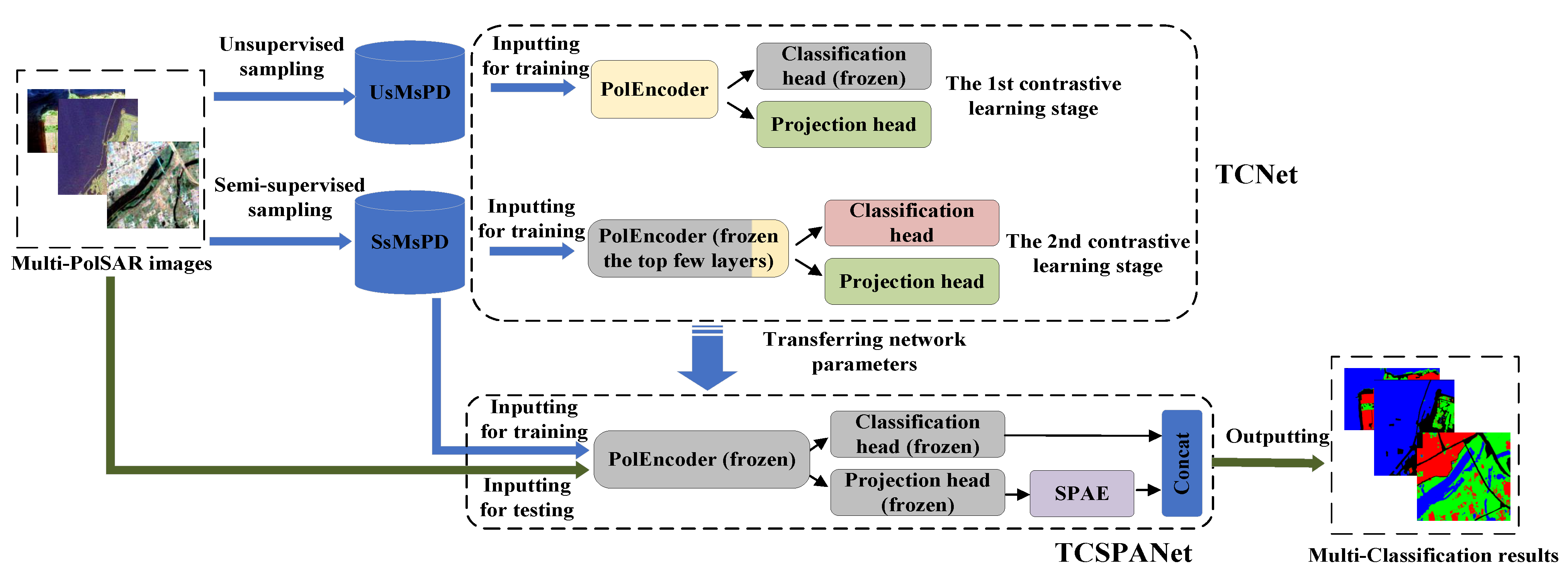
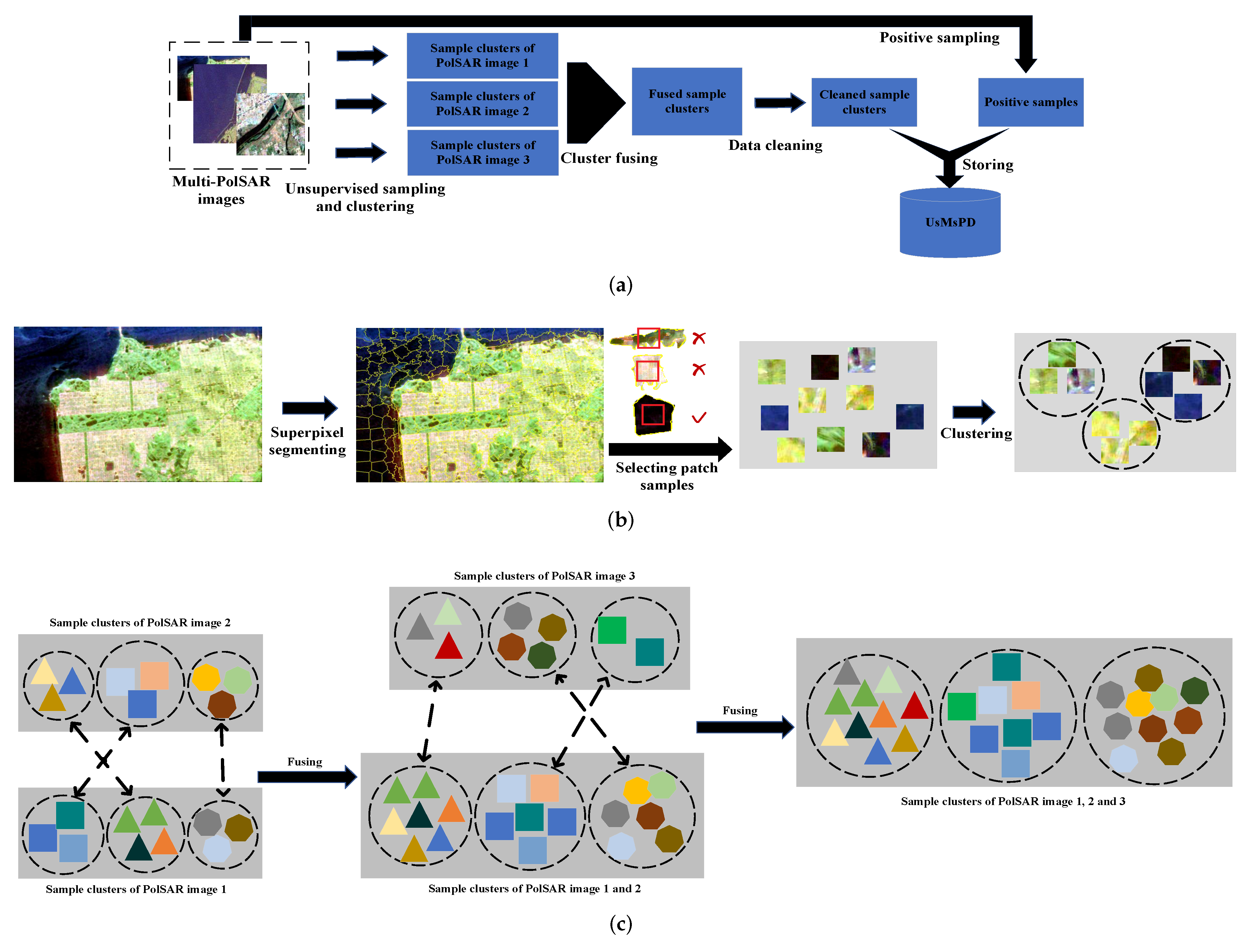
For the first contrastive learning stage of the TCNet, basing on multi-PolSAR images, we construct the dataset UsMsPD, consisting of patch samples of multi-scales, in an unsupervised manner. Figure 3a overviews how to establish the UsMsPD. Given a scale, firstly, patch samples are selected and clustered without supervision, conditioned on different PolSAR images. Secondly, clusters of all the PolSAR images are fused, so that each sample cluster contains multi-PolSAR images’ patches. Thirdly, we execute data cleaning for attaining more consistent clusters. Fourthly, the corresponding positive samples are picked from the multi-PolSAR images. Lastly, all these positive samples and their original samples are stored together to constitute the UsMsPD.

(1) Unsupervised sampling and clustering: Figure 3b displays how to receive and organize the qualified patch samples containing as few land cover categories as possible in an unsupervised manner. Simple linear iterative clustering (SLIC) [31] is a classical superpixel algorithm, which is fast, memory efficient and exhibits nice boundary adherence. So we resort to SLIC to segment a PolSAR image into individual superpixels. The Pauli scatter vector ${\mathbf{k}}_p=\frac{1}{\sqrt{2}}{\left[\begin{array}{ccc}{S}_{hh}+S_{vv}& S_{hh}-S_{vv}& 2S_{hv}\end{array}\right]}^{\top }$ is used to represent every pixel in conducting SLIC, where $S_{hv}$ means the scattering matrix element with the $h-v$ polarization of a receiving-transmitting wave (h and v are the notations of the horizon and vertical linear polarizations, respectively). After running SLIC in the PolSAR image $\rho$, we look at all the superpixels, and get the set ${\mathrm{X}}_{\rho }^{scal}$ of path samples with the specific scale $scal$, as follows:

$${\mathrm{X}}_{\rho }^{scal}=\left\{\mathbf{T}|\mathbf{T}\subset \mathbf{ST},\frac{\mathrm{size}\left(\mathbf{ST}\right)}{\mathrm{size}\left(\mathbf{T}\right)}>4\right\}$$

(1)

where $\rho$ refers to the PolSAR image segmented by SLIC; $scal$ means the scale of the selected patches; $\mathbf{T}\in {\mathbb{C}}^{scal\times scal\times 9}$ is the sampled complex-valued patch contained in the superpixel $\mathbf{ST}$ where every pixel is a coherency matrix, i.e., $\mathbf{T}\subset \mathbf{ST}$; $\mathrm{size}(·)$ is to calculate the number of pixels of a superpixel or a patch, so the second condition of (1) stipulates a superpixel must have above 4 times more pixels than the sampled patch it contains. As an unsupervised image segmentation algorithm, SLIC may produce a few under-segmented superpixels, where most heterogeneous pixels are far from central positions. To reduce the impact of under-segmented superpixels on the purity of the sampled patches, each patch is located in the center of whose corresponding superpixel which should possess more pixels than the sampled patch. The pixel multiple of a superpixel to its corresponding patch sample is consistent with the selection range (4 fold neighborhood) of a positive sample, so that both patches of a positive sample pair are covered by one superpixel as much as possible.

As mentioned before, it is not that arbitrary two patches can be negative samples of each other. Therefore, the popular Spetral Cluster [32] is leveraged to divide all the patches of the same size from the same PolSAR image into several clusters, where any two patches belonging to different clusters are regarded as negative samples of each other. Spectral Clustering uses a similarity matrix of all samples as the input. At first, we compute the Wishart distribution based distance [14]

$$d_w(i,j)=ln\left(|{\overline{\mathbf{T}}}_i|\right)+\mathrm{Tr}\left({\overline{\mathbf{T}}}_i^{-1}{\overline{\mathbf{T}}}_j\right)$$

(2)

for each two patch samples i and j, where ${\overline{\mathbf{T}}}_i$ and ${\overline{\mathbf{T}}}_j$ are the mean coherency matrixes of patch i and j, respectively. And then, the reciprocal of $d_w(i,j)$ is utilized to form the similarity matrix A, as follows:

$$\begin{array}{c}\hfill \mathcal{A}=\left(\frac{1}{d_w\left(i,j\right)}\right),\hfill \\ \hfill \mathbf{A}=\frac{\mathcal{A}+{\mathcal{A}}^{\top }}{2}\hfill \end{array}$$

(3)

It can be found from (2) that $d_w\left(i,j\right)\ne d_w\left(j,i\right)$, so the matrix $\mathcal{A}$ is asymmetric. In order to botain a symmetric similarity matrix and avoid the measurement inaccuracy caused by the asymmetry of $d_w(·,·)$, we carry out a simple and efficient average operation of $\mathcal{A}$ and its transpose. Finally, using $\mathbf{A}$, spectral clustering segments ${\mathrm{X}}_{\rho }^{scal}$ into $N_{scal}$ clusters. Performing the above operations on all the PolSAR images to be classified, several groups of sample clusters ${\mathrm{G}}_{\rho }^{scal}=\left\{{\mathrm{C}}_{\rho }^{scal,n}\right\}$ are achieved, where ${\mathrm{C}}_{\rho }^{scal,n}$ is the patch set of cluster n for PolSAR image $\rho$.

(2) Cluster fusing: After the previous operations, all the I PolSAR images to be classified are processed into $N_{scal}$ patch clusters separately. It is necessary to fuse these clusters into $N_{scal}$ larger clusters, each composed of clusters stemming from different PolSAR images, to use these samples in training the same model. It is clearly a stable matching problem, which can be solved by the Gale–Shapley algorithm [33], as follows:

$$\begin{array}{c}\hfill \left\{\begin{array}{cc}{\overline{\mathrm{C}}}_{\rho }^{scal}=\left\{\frac{1}{\left|{\mathrm{C}}_{\rho }^{scal,n}\right|}{\displaystyle \sum _{k=1}^{\left|{\mathrm{C}}_{\rho }^{scal,n}\right|}}{\overline{\mathbf{T}}}_{\rho ,k}^{scal,n}\right\},& \rho =1,...,I\\ {\mathrm{FC}}_2^{scal}=\mathrm{GS}\left({\overline{\mathrm{C}}}_1^{scal},{\overline{\mathrm{C}}}_2^{scal}\right)& \\ ⋮& \\ {\mathrm{FC}}_I^{scal}=\mathrm{GS}\left({\mathrm{FC}}_{I-1}^{scal},{\overline{\mathrm{C}}}_I^{scal}\right)& \end{array}\right.\end{array}$$

(4)

where, ${\overline{\mathrm{C}}}_{\rho }^{scal}$ is the set of vector representations of PolSAR image $\rho$ at scale $scal$, whose every element is the mean of all averaged coherency matrixes ${\overline{\mathbf{T}}}_{\rho ,k}^{scal,n}$ for cluster n; ${\mathrm{FC}}_I^{scal}$ is the final fused result, which is worked out by recursively executing Gale–Shapley algorithm $\mathrm{GS}\left(·,·\right)$ according to (4). In (4), the matching score of two clusters is computed through $1/d_w\left(i,j\right)$ to generate the “ranking matrix” according to [33] and get the matching result. Figure 3c is the diagram of cluster fusing. In the execution of cluster fusing, the ordering of patch clusters also matters. We should first fuse the clusters of images containing more samples. In the first few steps of fusion, the size of one cluster has a great influence on its representation. Clusters with fewer samples may be more easily affected by some bad samples, leading to inconsistent matching of clusters, and finally result in an unreasonable fusion, and even hinder the network from learning the intrinsic representation of PolSAR images. At the later stage of fusion, the fusion will be more robust to the small clusters because larger clusters have been generated.

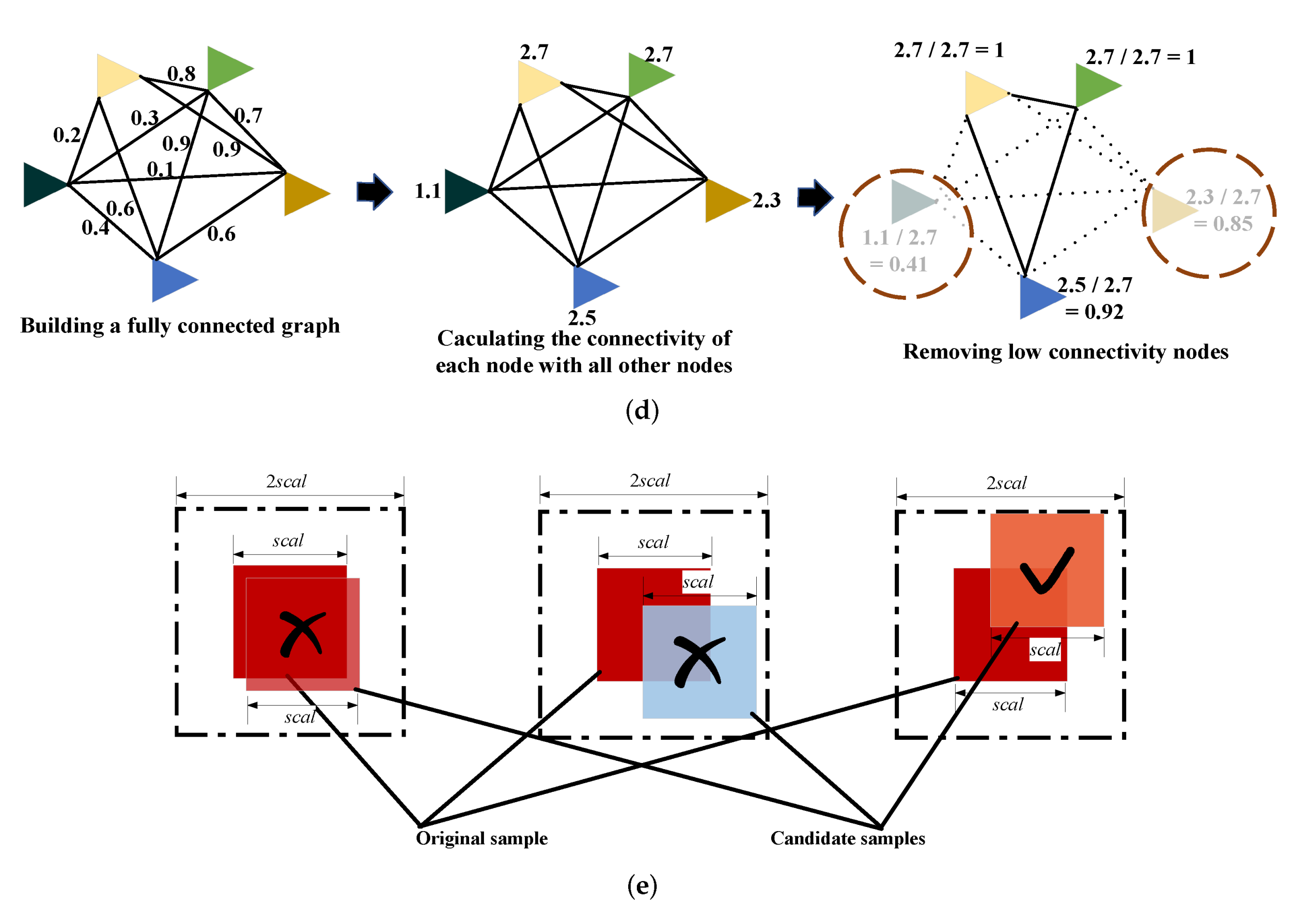
(3) Data cleaning: To keep the patch samples of the same cluster consistent, the “outlier samples” that differ greatly from the others should be removed through data cleaning. Figure 3d demonstrates the procedure of data cleaning for one fused cluster. Firstly, we build a fully connected graph with all patch samples as the nodes by (3). Next, the connectivity of each node is acquired by summing all the connection weights between it and the other nodes. Then, we find the node of the highest connectivity, and compute the ratio of each node’s connectivity to the highest value. Finally, by removing the nodes with a connectivity ratio below the predefined threshold, the ultimate “fairly clean” clusters are acquired.

(4) Positive sampling: In order not to destroy the polarization characteristics of the sampled PolSAR patches, we do not construct positive sample pairs by data augmentation. It is also unreasonable to directly view a cluster’s image patches as positive samples of one another because they still possibly belong to different land cover types. Our scheme is to collect positive samples near the original ones. The two patches that make up a positive sample pair should near to each other in polarization space and include as few duplicate pixels. To this end, we put forward a mixed distance, as follows:

$$d_m\left(i,j\right)=d_w\left(i,j\right)-\lambda \sqrt{{\left(v{c}_i-v{c}_j\right)}^2+{\left(h{c}_i-h{c}_j\right)}^2}$$

(5)

where the first term is the Wishart distribution based distance as (2), the second term represents the spatial distance, $v{c}_i$ (or $v{c}_i$) and $h{c}_i$ (or $h{c}_j$) are the vertical and horizontal coordinates for the center of patch sample i (or j), respectively, and $\lambda >0$ (we set $\lambda =0.1$ in this article) is the hyper-parameter to control the contribution of spatial distance to the mixed distance. For any patch $\mathbf{T}$ sampled before, in its four times area neighbourhood, a certain number of new image patches ${\mathbf{T}}^{\#}$ are sampled as the set of its candidate positive samples, in which the candidate sample has minimum mixed distance to $\mathbf{T}$ is chosen as the positive sample ${\mathbf{T}}^{+}$, as follows:

$${\mathbf{T}}^{+}=\underset{{\mathbf{T}}^{\#}}{argmin}\left(d_m\left(\mathbf{T},{\mathbf{T}}^{\#}\right)\right)$$

(6)

Figure 3e shows three relationships between an original sample and its candidate samples. The left two patches are too close in spatial space and have lots of the same pixels. The middle two patches are too far away in polarization characteristics and may belong to different land covers. The right two patches are neither too close in spatial space nor far away in polarization characteristics and have the minimum mixed distance, which can be positive samples of each other. Besides, four times neighbourhood restricts every pair of positive samples to one superpixel, reducing the risk that the two samples containing different land covers due to the extremely large spatial distance.

The previous operations are under a single value of $scale$. For the UsMsPD, $scal\in \left\{32,16,8,4,2\right\}$. As stated at the beginning of this section, for learning the purity of a patch sample, the context inside a patch can be modeled by extracting the dependence in the sub-patches of this patch (the specific procedure will be described later). Although a $2\times 2$ patch can continue to be evenly split into four smaller sub-patch, i.e., four pixels, their dependence is not enough to reflect the purity of the $2\times 2$ patch. Because individual pixels are susceptible to noise. Therefore, we define $2\times 2$ as the smallest sample scale, that is, the minimum  of  $scal$  is  2. 

Using all the optional $scal$, we get the entire unsupervised multi-scaled patch-level dataset, UsMsPD.

3.1.2. Semi-Supervised Multi-Scale Patch-Level Dataset

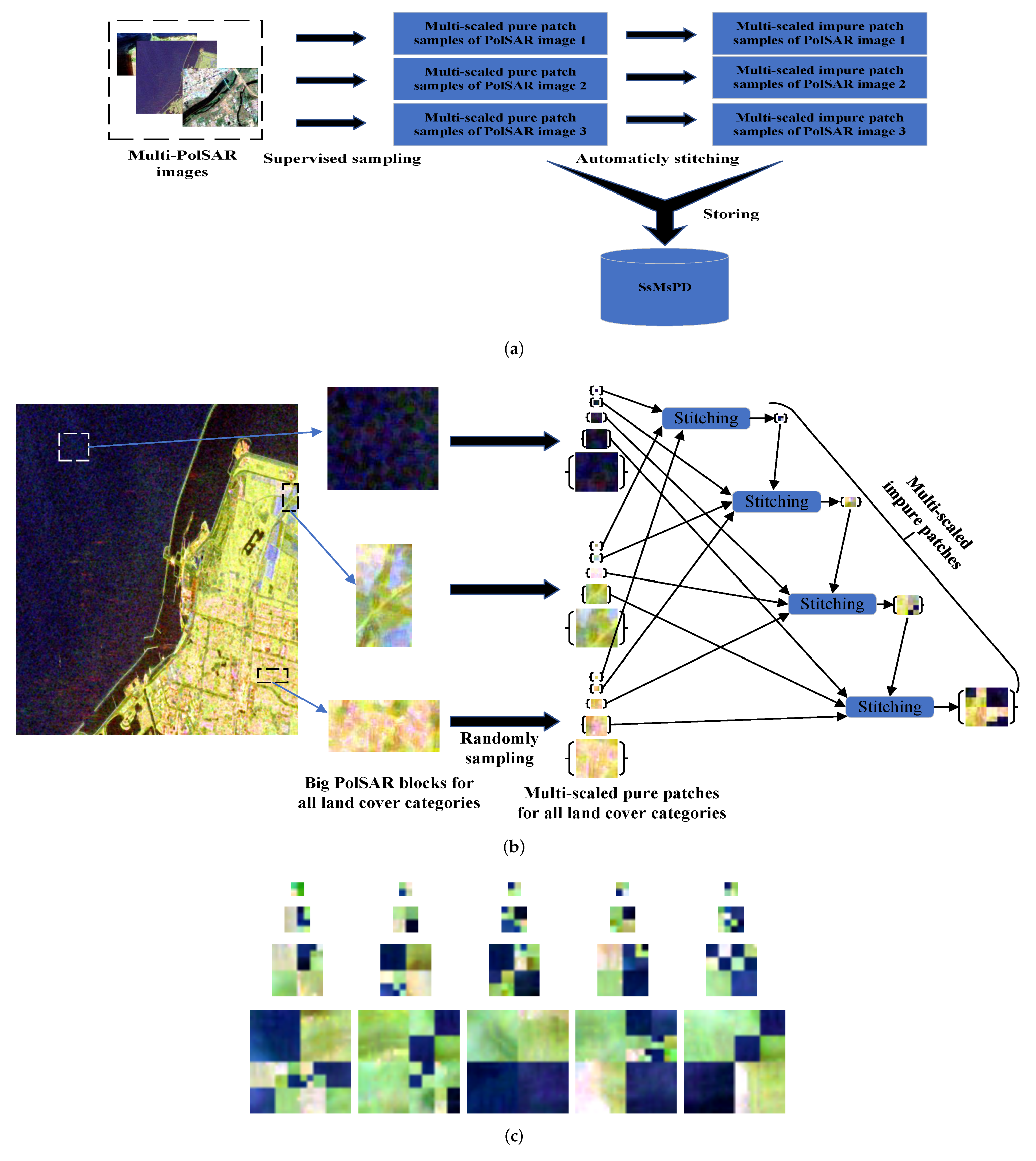
It is essential to establish the dataset SsMsPD, including category labels, to make the network gain discrimination capability for concrete land cover categories, which cannot be learned from the UsMsPD. In realistic application, an entire PolSAR image cannot be classified satisfactorily with only one scale of patches, so the dataset should contain multi-scaled patches. In addition, when predicting, it cannot be ensured that all patches contain only one land cover. The annotated patch-level dataset SsMsPD should include two kinds of patch samples: the patches only contain one type of land cover, i.e., pure patches; the patches contain two or more land cover categories, i.e., impure patches. As is shown in Figure 4a, in the SsMsPD, the pure patches are collected by hand, while the impure patches are automatically generated. Thus, the SsMsPD is obtained in a semi-supervised way.

Figure 4b is the specific sampling and generating process from one PolSAR image in Figure 4a. Firstly, some big PolSAR blocks are selected manually, each corresponding to a land cover category. And then, multi-scaled pure patches ${\mathbf{T}}_{\rho }^{scal}$ are randomly sampled from these blocks. All the pure patches from the same big block share the same land cover category, thus their labels $\mathbf{y}\left({\mathbf{T}}_{\rho }^{scal}\right)$ are given. Here, $\rho$ and $scal\in \left\{32,16,8,4,2\right\}$ are defined before. Next, impure patches ${\tilde{\mathbf{T}}}_{\rho }^{scal}$ are generated based on smaller pure patches ${\mathbf{T}}_{\mathbf{\ae }}^{\mathit{scal}/\mathbf{2}}$ and impures patches ${\tilde{\mathbf{T}}}_{\mathbf{\ae }}^{\mathit{scal}/\mathbf{2}}$, as follows:  

$$\begin{array}{c}\hfill {\tilde{\mathbf{T}}}_{\rho }^{scal}=\mathrm{ST}\left({\mathbf{T}}_{\rho ,1}^{*scal/\phantom{*scal2}2},{\mathbf{T}}_{\rho ,2}^{*scal/\phantom{*scal2}2},{\mathbf{T}}_{\rho ,3}^{*scal/\phantom{*scal2}2},{\mathbf{T}}_{\rho ,4}^{*scal/\phantom{*scal2}2}\right),\\ \hfill s.t.\left\{\begin{array}{c}scal\in \left\{4,8,16,32\right\}\\ {\mathbf{T}}_{\rho }^{*scal/\phantom{*scal2}2}=\begin{array}{ccc}{\mathbf{T}}_{\rho }^{scal/\phantom{scal2}2}& or& {\tilde{\mathbf{T}}}_{\rho }^{scal/\phantom{scal2}2}\end{array}\\ \neg \left(\mathbf{y}\left({\mathbf{T}}_{\rho ,1}^{scal/\phantom{scal2}2}\right)=\mathbf{y}\left({\mathbf{T}}_{\rho ,2}^{scal/\phantom{scal2}2}\right)\right.\\ \left.=\mathbf{y}\left({\mathbf{T}}_{\rho ,3}^{scal/\phantom{scal2}2}\right)=\mathbf{y}\left({\mathbf{T}}_{\rho ,4}^{scal/\phantom{scal2}2}\right)\right)\end{array}\right.\end{array}$$

(7)

where $\mathrm{ST}\left(·,·,·,·\right)$ represents stitching four patches into a larger impure patch; the first condition suggests that impure patches have only four scales to choose from, i.e., $scal\ne 2$; the second condition means the smaller patch-level samples used in $\mathrm{ST}$ contain pure patches and impure patches; the third condition avoids that an impure patch is stitched by four pure patches that have the same land cover category. In the actual implementation, smaller impure patches must be generated earlier in order that they can be used in generating larger impure patches. Thus, see Figure 4c, the larger an impure patch is, the more complex its land cover is.

3.2. Two-Staged Contrastive Learning and Sub-Patch Attention Based Network

In this subsection, we propose a novel PolSAR image classification model TCSPANet. As is shown in Figure 1, the TCSPANet is constructed gradually by updating the TCNet and the SPAE in turn with the datasets UsMsPD and SsMsPD presented before.

3.2.1. Two-Staged Contrastive Learning Based Network

(1) Structure of the TCNet: Inspired by the simplicity and scalability of simCLR, we construct the TCNet, whose structure is shown in Figure 5a. Unlike the simCLR, in addition to the base encoder (we call it PolEncoder) and the projection head, a classification head is also introduced.

For extracting the representation vectors from PolSAR images, we establish a small neural network PolEncoder $f\left(·\right)$. First of all, an input patch $\mathbf{T}$ is tiled to the size of $32\times 32$, denoted by $\mathrm{Tile}\left(\mathbf{T}\right)$, to meet the input requirement of $f\left(·\right)$. Then, complex-valued convolutions (CV-CNNs) [34], the operation is defined in (1) and (2) of [34], are used to mine features in complex filed; max poolings are adopted to reduce the size of feature maps and improve the translation and rotation invariance of CV-CNNs; a global average pooling is to compress the final feature maps C4 into a vector; two full connection layers further encode the features of CV-CNN to a representation vector. In the PolEncoder, we utilize Relu [35] as the active function to enhance the approximation capability. So, the output of the PolEncoder is ${\mathbf{h}}_i=f\left(\mathrm{Tile}\left({\mathbf{T}}_i\right)\right)$ where ${\mathbf{T}}_i\in {\mathbb{C}}^{scal\times scal\times 9}$ is the complex-valued input patch, ${\mathbf{h}}_i\in {\mathbb{R}}^{240}$ is the output of the PolEncoder f.

The projection head $g(·)$ maps representations got by $f(·)$ to a space where a new contrastive loss is applied. Like the simCLR, the projection head is also a multilayer perception (MLP) with one full connection layer to obtain the projection vector ${\mathbf{z}}_i=g\left({\mathbf{h}}_i\right)$. The classification head $b(·)$ is just a layer of full connection with a softmax function, which converts the output of the PolEncoder to vector ${\mathbf{v}}_i=b\left({\mathbf{h}}_i\right)$ where ${\mathbf{v}}_i\in {\mathbb{R}}^M$ corresponds to the land cover category $\mathbf{y}\left({\mathbf{T}}_i\right)$.

(2) Training the TCNet: As is shown in Figure 5b,c, the TCNet is trained with two stages. Figure 5b shows that, in the first contrastive learning stage, the PolEncoder and the projection head are trained on the UsMsPD. In light of the fact that there is no category information in the UsMsPD, updating the classification head’s parameters does not make sense. Hence, the classification head is frozen in this training stage. Given a scale $scal$ for the patch samples in the UsMsPD, $2N_{scal}$ samples are inputted into the network, where the top $N_{scal}$ samples are from different clusters and the next $N_{scal}$ samples are their positive samples. What is more, if $scal>2$, one more patch ${\mathbf{T}}_{2N+1}$ is inputted into the TCNet. ${\mathbf{T}}_{2N_{scal}+1}$ is not any sample of the UsMsPD. Instead, it is stitched by the central patches of stochastic four in the top $2N_{scal}$ samples. In this way, ${\mathbf{T}}_{2N_{scal}+1}$ is the negative sample of all the top $2N_{scal}$ patches. Then the loss function for a positive pair of examples $(i,j)$, the normalized temperature-scaled cross entropy loss (NT-Xent) in [11] is modified as the extended NT-Xent (ENT-Xent) in this article:  

$$l_{i,j,scal}=\left\{\begin{array}{cc}-log\frac{exp\left(sim\left({\mathbf{z}}_i,{\mathbf{z}}_j\right)/\tau \right)}{{\displaystyle \sum _{k=1}^{2N_{scal}}}{⊮}_{\left[k\ne i\right]}exp\left(sim\left({\mathbf{z}}_i,{\mathbf{z}}_k\right)/\tau \right)},& scal=2\\ -log\frac{exp\left(sim\left({\mathbf{z}}_i,{\mathbf{z}}_j\right)/\tau \right)}{{\displaystyle \sum _{k=1}^{2N_{scal}+1}}{⊮}_{\left[k\ne i\right]}exp\left(sim\left({\mathbf{z}}_i,{\mathbf{z}}_k\right)/\tau \right)},& scal>2\end{array}\right.$$

(8)

where all symbols are defined in the same way as NT-Xent in [11]. The only difference is that our ENT-Xent has an extra $exp\left(sim\left({\mathbf{z}}_i,{\mathbf{z}}_{2N_{scal}+1}\right)/\tau \right)$ in the denominator when $scal>2$, which guarantees that the extra input is pushed away from all the other samples. Accordingly, the total contrastive loss for a batch of inputs is

$$L_C=\frac{1}{2N_{scal}}\sum _{k=1}^{2N_{scal}}\left[l_{2k-1,2k}+l_{2k,2k-1}\right].$$

(9)

Figure 5b shows the second stage of training for the TCNet, when the TCNet is further trained with our proposed SsMsPD to acquire the discriminant ability for actual land cover categories During this stage, all the layers of the encoder except the last two are frozen. Given a scale $scal=2$, M pairs of pure patches, all pairs marked as different land cover categories, are inputted into the TCNet. When $scal>2$, an impure patch ${\tilde{\mathbf{T}}}_{2M+1}$ is also an input data in one batch. All the representations ${{\mathbf{T}}^{*}}_1\sim {{\mathbf{T}}^{*}}_{2M\mathrm{or}2M+1}$ are then inputted into $g(·)$ to get the corresponding projection vectors ${\mathbf{z}}_1\sim {\mathbf{z}}_{2M\mathrm{or}2M+1}$. The loss function for $g(·)$ is defined in (8) and (9), where $N_{scal}$ is replaced with M. The representations of pure patches ${{\mathbf{T}}^{*}}_1\sim {{\mathbf{T}}^{*}}_{2M}\left(scal=2\right)$ are also inputted into $b(·)$ to get classification vectors ${\mathbf{v}}_1\sim {\mathbf{v}}_{2M}$. The loss function for the classification head is the classical categorical cross entropy:

$$L_{CE}=-\frac{1}{2M}\frac{1}{M}\sum _{i=1}^{2M}\sum _{k=1}^M{\mathbf{y}}_i^{k}ln\left({\mathbf{v}}_i^k\right).$$

(10)

Finally, the total loss function for the second contrastive learning stage of the TCNet is a weighted sum of $L_C$ and $L_{CE}$:

$$L_1=\gamma L_C+\left(1-\gamma \right)L_{CE}$$

(11)

where $\gamma$ and $1-\gamma$ are the weights for the two losses. In this article, $\gamma =0.5$ to align projection head and classification head the same significance.

It can be found that the emphases of the two stages of contrastive learning are distinct. In the first contrastive learning stage, the TCNet focuses on extracting effective representations of PolSAR image patches with the unlabeled dataset. In the second contrastive learning stage, the TCNet aims at learning categorical information and obtaining comparability for actual land covers by inputting samples that are annotated with real land cover classes. Moreover, both in the two training stages, one more patch sample is inputted into the TCNet if $scal$ is not the minimum, enabling the TCNet to push impure patches far away from any pure patch.

3.2.2. Sub-Patch Attention Encoder

(1) Integrating the SPAE into the trained TCNet: Figure 4c suggests that impure patches in the SsMsPD do not have any specific pattern, which cannot be directly considered a new land cover category and classified by the TCNet. If a patch is evenly split into four sub-patches and inputted into the trianed TCNet, one the following two situations will occur: for a pure patch, the projection vectors of its four sub-patches will be similar; for an impure patch, there must be some difference among the four sub-patches’ projection vectors. The context within a patch can be modelled through capturing the dependence of the four sub-patches in a patch samples, which can be utilized to judge whether a patch is pure patch or impure patch. For this purpose, we put forward the SPAE. By plugging the SPAE into the trained TCNet, we get the final model TCSPANet. Figure 6a shows how to optimize the SPAE to get the available TCSPANet. For a patch sample from the SsMdPD, it is divided into two parts of input: the first part of input is the patch itself, ${\mathbf{T}}_i^{*}$; the second part are the four sub-patches $\mathbf{s}{\mathbf{T}}_{i,1}\sim \mathbf{s}{\mathbf{T}}_{i,4}$, the evently split result of ${\mathbf{T}}_i^{*}$. The complete patch ${\mathbf{T}}_i^{*}$ is inputed into the trained PolEncoder to get its representation vector ${\mathbf{h}}_i=f\left({\mathbf{T}}_i^{*}\right)$, and then is converted into the classification vector ${\mathbf{v}}_i=b\left({\mathbf{h}}_i\right)$ with the trained classification head frozen and without Softmax. The four sub-patches are inputted into the same PolEncoder to obtain their representations ${\mathbf{sh}}_{\mathit{i},\mathbf{1}}\sim {\mathbf{sh}}_{\mathit{i},\mathbf{4}}$, which are then mapped to four projection vectors $\mathbf{s}{\mathbf{z}}_{i,1}\sim \mathbf{s}{\mathbf{z}}_{i,4}$ (we call them sub-patch tokens here). The sub-patch tokens are stacked together to form a matrix $\mathbf{s}{\mathbf{Z}}_i\in {\mathbb{R}}^{4\times 240}=[\mathbf{s}{\mathbf{z}}_{i,1};...;\mathbf{s}{\mathbf{z}}_{i,4}]$ as the input of the SPAE $u(·)$. Next, the context within the completed patch is encoded to a scalar ${\epsilon }_i=u\left({\mathbf{sZ}}_{\mathit{i}}\right)$. The outputs of the SPAE and the classification head are merged and normalized by a softmax function to get the final output of the TCSPANet, as follows:

$$\begin{array}{cc}\hfill {\stackrel{⌢}{\mathbf{y}}}_i& =\mathrm{TCSPANet}\left({\mathbf{T}}_i^{*},\mathbf{s}{\mathbf{T}}_1,\mathbf{s}{\mathbf{T}}_2,\mathbf{s}{\mathbf{T}}_3,\mathbf{s}{\mathbf{T}}_4\right)\hfill \\ & =\mathrm{softmax}\left(\left[b\left(f\left({\mathbf{T}}_i^{*}\right)\right),\right.\right.\hfill \\ & \left.\mu \left(\left[g\left(f\left(\mathbf{s}{\mathbf{T}}_1\right)\right);g\left(f\left(\mathbf{s}{\mathbf{T}}_2\right)\right);g\left(f\left(\mathbf{s}{\mathbf{T}}_3\right)\right);g\left(f\left(\mathbf{s}{\mathbf{T}}_4\right)\right)\right]\right)\right]\hfill \\ & =\mathrm{softmax}\left(\left[b\left({\mathbf{h}}_i\right),\mu \left({\mathbf{sZ}}_i\right)\right]\right)\hfill \\ & =\mathrm{softmax}\left(\left[{\mathbf{v}}_i,{\epsilon }_i\right]\right)\hfill \end{array}$$

(12)

where ${\stackrel{⌢}{\mathbf{y}}}_i\in {\mathbb{R}}^{M+1}$ is the final output of the TCSPANet. In (12), only u(·) an be optimized, while f(·), g(·), b(·) are fixed after training the TCNet.

The categorical cross entropy is used again as the loss function to update the SPAE.

$$L_2=-\frac{1}{B}\frac{1}{M+1}\sum _{i=1}^B\sum _{k=1}^{M+1}{\dot{\mathbf{y}}}_i^{k}ln\left({\stackrel{⌢}{\mathbf{y}}}_i^k\right)$$

(13)

where B means the batch size, $\dot{\mathbf{y}}\in {\mathbb{R}}^{M+1}$ is the new label for the patch sample ${\mathbf{T}}^{*}$, defined as follows:

$$\dot{\mathbf{y}}\left({\mathbf{T}}^{*}\right)=\left\{\begin{array}{cc}\left[\mathbf{y}\left({\mathbf{T}}^{*}\right),0\right],\hfill & {\mathbf{T}}^{*}\mathrm{is}\mathrm{a}\mathrm{pure}\mathrm{patch}\\ \left[0,...,0,1\right],\hfill & {\mathbf{T}}^{*}\mathrm{is}\mathrm{an}\mathrm{impure}\mathrm{patch}\end{array}\right.$$

(14)

$\dot{\mathbf{y}}\left({\mathbf{T}}^{*}\right)$ tells that whether ${\mathbf{T}}^{*}$ is an impure patch or which category the patch belongs to when a pure patch.

(2) Structure of the SPAE: The structure of the SPAE is shown in Figure 6b, which is composed of two sub-structures, a transformer encoder and a sub-patch attention extractor based on CNN. In our opinion, the context of sup-patches exists explicitly in attention maps in every transformer layer. And then, these attention maps are stacked and further processed to a scalar value ${\epsilon }_i$ by the sub-patch attention extractor as the final output of the entire SPAE.

The transformer encoder consists of E layers of small networks that include multi-head attention (MHA) and MLP blocks. L2 normalization is adopted before and after every MHA block. The MLP contains two layers of full connection with a Relu non-linearity. Different from the original transformer, we omit positional encoding which is not concerned in our model.

In each layer l, MHA allows the SPAE to attend to the context within the input $\mathbf{s}{\mathbf{Z}}_i^{\left(l-1\right)}$ in different projection subspaces.

$$\begin{array}{cc}\hfill & \mathrm{MHA}\left(\mathrm{Norm}\left(\mathbf{s}{\mathbf{Z}}_i^{\left(l-1\right)}\right)\right)=\mathrm{Concat}\left({\mathrm{head}}_1,...,{\mathrm{head}}_{\underline{h}}\right){\mathbf{W}}^{\left(l\right)O}\hfill \\ \hfill & {\mathrm{head}}_j=\mathrm{Attention}\left(\mathrm{Norm}\left(\mathbf{s}{\mathbf{Z}}_i^{\left(l-1\right)}\right){\mathbf{W}}_j^{\left(l\right)Q},\right.\hfill \\ \hfill & \left.\mathrm{Norm}\left(\mathbf{s}{\mathbf{Z}}_i^{\left(l-1\right)}\right){\mathbf{W}}_j^{\left(l\right)K},\mathrm{Norm}\left(\mathbf{s}{\mathbf{Z}}_i^{\left(l-1\right)}\right){\mathbf{W}}_j^{\left(l\right)V}\right)\hfill \\ \hfill & =\mathrm{Attention}\left({\mathbf{Q}}_j^{\left(l\right)},{\mathbf{K}}_j^{\left(l\right)},{\mathbf{V}}_j^{\left(l\right)}\right)\hfill \end{array}$$

(15)

where ${\mathbf{W}}_j^{\left(l\right)Q}$, ${\mathbf{W}}_j^{\left(l\right)K}$, ${\mathbf{W}}_j^{\left(l\right)V}\in {\mathbb{R}}^{240\times 240/\underline{h}}$, ${\mathbf{W}}_j^{\left(l\right)O}\in {\mathbb{R}}^{240\times 240}$ are the linear projection matrices in the head j to obtain the triple (query ${\mathbf{Q}}_j^{\left(l\right)}$, key ${\mathbf{K}}_j^{\left(l\right)}$, value ${\mathbf{V}}_j^{\left(l\right)}$) and the output of the MHA. The attention for every head is formulated as follows:

$$\mathrm{Attention}\left({\mathbf{Q}}_j^{\left(l\right)},{\mathbf{K}}_j^{\left(l\right)},{\mathbf{V}}_j^{\left(l\right)}\right)=\mathrm{softmax}\left(\frac{{\mathbf{Q}}_j^{\left(l\right)}\mathbf{K}{{}_j^{\left(l\right)}}^{\top }}{\sqrt{d_k}}\right){\mathbf{V}}_j^{\left(l\right)}$$

(16)

where $d_k$ is the length of each sequence in ${\mathbf{K}}_j^{\left(l\right)}$. $\mathrm{Norm}(·)$ is used to normalized every sequence of a matrix.

$$\mathrm{Norm}\left({\mathbf{sZ}}_i^{\left(0\right)}\right)=\left[\frac{\mathbf{s}{\mathbf{z}}_{i,1}}{∥\mathbf{s}{\mathbf{z}}_{i,1}∥};\dots ;\frac{\mathbf{s}{\mathbf{z}}_{i,4}}{∥\mathbf{s}{\mathbf{z}}_{i,4}∥}\right]$$

(17)

Then the output of the current transformer is projected from the output of the MHA block.

$$\begin{array}{cc}\hfill & {{\mathbf{sZ}}^{\prime }}_i^{\left(l\right)}=\mathrm{MHA}\left(\mathrm{Norm}\left({\mathbf{sZ}}_i^{\left(l-1\right)}\right)\right)+{\mathbf{sZ}}_i^{\left(l-1\right)}\hfill \\ \hfill & {\mathbf{sZ}}_i^{\left(l\right)}=\mathrm{MLP}\left(\mathrm{Norm}\left({{\mathbf{sZ}}^{\prime }}_i^{\left(l\right)}\right)\right)+{{\mathbf{sZ}}^{\prime }}_i^{\left(l\right)}\hfill \end{array}$$

(18)

where $\mathbf{s}{\mathbf{Z}}_i^{\left(l\right)}$ is the output transformer layer l, which is the input of the layer $l+1$.

Next, we take each sub-patch attention map ${\mathbf{SPAM}}_j^{\left(l\right)}\in {\mathbb{R}}^{4\times 4}=\mathrm{softmax}\left(\frac{{\mathbf{Q}}_j^{\left(l\right)}{\mathbf{K}}_j^{\left(l\right)}}{\sqrt{d_k}}\right)$ corresponding to every transformer layer l and head j, and stack them to form the sub-patch attention maps $\mathbf{SPAM}\in {\mathbb{R}}^{4\times 4\times hE}$ as the input of the sub-patch attention extractor $\mathcal{C}(·)$. $\mathcal{C}(·)$ is a CNN based network composed of two convolution layers with Relu, a maxpooling layer and full connection layer without non-linearity. Adoptting $\mathcal{C}(·)$, we compress the matrix $\mathbf{SPAM}$ into a scalar value $\epsilon \in \mathbb{R}=\mathcal{C}\left(\mathbf{SPAM}\right)$ as the representation of the overall self-attention for all sub-patches.

3.2.3. Training the TCSPANet

Figure 1 demonstrates that not all components’ parameters in the TCSPANet can be updated throughout the training process. When training the TCNet, all parameters of the PolEncoder except the final two layers are fixed in the second contrastive learning stage so that the PolEncoder can mine intrinsic PolSAR information effectively and also learn the representation for real land cover categories. The classification head is trained in the second contrastive learning stage of the TCNet to guide the optimization of the PolEncoder with supervision. The projection head is trained in both two contrastive learning stages of the TCNet. During training the TCSPANet, only the SPAE is refreshed for modeling the context within patch samples. In summary, it is a kind of progressive learning [36,37] to train the TCSPANet. See Appendix A for the algorithm of training the TCSPANet.

3.2.4. Classifying or Splitting

In this paper, a novel non-overlapping coarse-to-fine patch-level classification algorithm, classifying or splitting, is proposed for completed PolSAR images. For a patch for one PolSAR image to be classified, the trained TCSPANet first determines whether it is a pure patch or an impure patch. If the TCSPANet regards the patch as a pure patch, its terrain category will be provided immediately (i.e., classifying step). Conversely, if the patch is viewed as an impure patch, it will be evenly split into four smaller patches and reinputted into the TCSPANet for further recognizing (i.e., splitting step). The above steps are repeated until the entire PolSAR image is classified. When running classifying and splitting, larger patches are selected in homogeneous regions while smaller patches are chosen in complicated areas. The blocking effect is effectively alleviated. Meanwhile, non-overlapping of patches improves computation efficiency. The pseudocode of classifiying or splitting is displayed in Appendix B.

4. Experimental Results

4.1. Description of Datasets

The experiments are performed on three different PolSAR images, which are from different sites, received by different sensors, and have the same categories of land covers. The first PolSAR image is in San Francisco, a city in the USA. It was received by AIRSAR and has $935\times 1369$ pixels. The second PolSAR image is in Flevoland, Netherlands. It was acquired by RADARSAT-2, and its size is $1379\times 1093$. The next PolSAR image is from Xi’an, the capital city of Shaanxi province in China. It is captured by SIA_C/X-SAR and includes $512\times 512$ points. Figure 7a–f show the PauliRGB images and ground truths for the three images. Each image has the same three land cover categories: water, vegetation, and urban. Figure 7g gives the color code for the three categories.

Based on the three PolSAR images, two datasets, UsMsPD and SsMsPD, are built up. For each category in every PolSAR image, a big block is selected, where multi-scaled pure patches are sampled to construct the SsMsPD. Figure 8 marks these big blocks, whose coordinates are shown in

Table 1. Big Blocks for Different Categories in Multi-PolSAR images.

PolSAR	Water		Vegetation		Urban
	Coordinates	Annotation Proportion	Coordinates	Annotation Proportion	Coordinates	Annotation Proportion
San Francisco	(1:100,1:100)	4.86%	(117:167,429:529)	9.44%	(256:356,567:667)	2.92%
Flevoland	(245:345,390:490)	1.12%	(342:442,1042:1092)	6.18%	(826:876,785:885)	4.96%
Xi’an	(353:403,42:92)	6.80%	(8:108,429:479)	4.18%	(177:227,60:110)	3.08%

.

4.2. Experimental Design

For verifying the proposed TCSPANet, several classical and state of the art methods are compared with our method, including four machine learning-based approaches, including support vector machine (SVM) [38] and Wishart [39], Random Forest (RF) [40] and EXtreme Gradient Boosting (XGBoost) [41], and five deep learning-based methods, including stacked sparse autoencoder (SAE) [42], deep belief network (DBN) [4] CV-CNN [34], densely connected and depthwise separable convolutional neural network (DSNet) [43] and Spatial feature-based convolutional neural network (SF-CNN) [44]. DSNet and SF-CNN are the state of the art deep learning based models for PolSAR classification, where DSNet retains features in shallow layers through dense connection, SF-CNN combines K-Nearest Neighbor (KNN) with deep learning network to near samples with the same class yet make samples of different classes far away. All these methods are trained once with the dataset constructed based on multi-PolSAR images, and tested on the three images. In our TCSPANet, we set $\tau =0.1$ which brings the best results in [11], $\gamma =0.5$ to treat projection head and classification head equally, and the number of both heads and layers in the transformer encoder of the SPAE is three. For every method, we figure out  the  accuracy  (ACC)  of  each  category,  overall  accuracy  (OA)   and   Kappa  coefficient (Kappa) [45]. After ten experiments, the means and variances of the evaluation metrics are shown in

Table 2. Classification Results of San Francisco with Different Methods, where the highest mean and lowest variance for each category are marked in bold.

Method	Water	Vegetation	Urban	OA	Kappa
SVM	0.9996 ± 1.2744 × 10${}^{-11}$	0.7408 ± 4.3960 × 10${}^{-5}$	0.8622 ± 6.1643 × 10${}^{-6}$	0.9046 ± 1.3737 × 10${}^{-6}$	0.8140 ± 7.6377 × 10${}^{-6}$
Wishart	0.9382 ± 1.6538 × 10${}^{-11}$	0.8548 ± 4.3550 × 10${}^{-9}$	0.7102 ± 1.1253 × 10${}^{-8}$	0.8009 ± 2.8625 × 10${}^{-9}$	0.6835 ± 4.7917 × 10${}^{-9}$
RF	0.9425 ± 1.3935 × 10${}^{-5}$	0.5846 ± 3.0230 × 10${}^{-3}$	0.9703 ± 4.6518 × 10${}^{-5}$	0.9180 ± 9.9175 × 10${}^{-5}$	0.8549 ± 2.4030 × 10${}^{-4}$
XGBoost	0.9971 ± 8.3084 × 10${}^{-8}$	0.6991 ± 3.1952 × 10${}^{-5}$	0.9360 ± 1.8346 × 10${}^{-6}$	0.9381 ± 1.9231 × 10${}^{-7}$	0.8864 ± 7.1646 × 10${}^{-7}$
SAE	0.9975 ± 6.1816 × 10${}^{-7}$	0.5208 ± 1.7738 × 10${}^{-3}$	0.9064 ± 2.0067 × 10${}^{-4}$	0.9032 ± 6.3105 × 10${}^{-5}$	0.8227 ± 2.1584 × 10${}^{-4}$
DBN	0.7609 ± 2.5562 × 10${}^{-3}$	0.3608 ± 2.6251 × 10${}^{-4}$	0.9785 ± 1.3553 × 10${}^{-5}$	0.8404 ± 3.3678 × 10${}^{-4}$	0.7164 ± 1.0713 × 10${}^{-3}$
CV-CNN	0.9658 ± 8.2194 × 10${}^{-5}$	0.1098 ± 6.0291 × 10${}^{-2}$	0.9936 ± 2.0359 × 10${}^{-5}$	0.9063 ± 2.5394 × 10${}^{-4}$	0.8168 ± 1.1516 × 10${}^{-3}$
DSNet	0.9998 ± 1.2924 × 10${}^{-7}$	0.8830 ± 1.2248 × 10${}^{-3}$	0.8856 ± 1.4197 × 10${}^{-3}$	0.9201 ± 7.8113 × 10${}^{-4}$	0.8470 ± 3.1580 × 10${}^{-3}$
SF-CNN	0.9722 ± 1.1009 × 10${}^{-3}$	0.2631 ± 9.8136 × 10${}^{-4}$	0.9598 ± 2.3465 × 10${}^{-4}$	0.7880 ± 4.3201 × 10${}^{-4}$	0.6637 ± 8.9135 × 10${}^{-4}$
Our method	0.9620 ± 7.3259 × 10${}^{-5}$	0.7851 ± 2.1159 × 10${}^{-3}$	0.9596 ± 3.2721 × 10${}^{-5}$	0.9451 ± 1.9813 × 10${}^{-5}$	0.9008 ± 6.5051 × 10${}^{-5}$

,

Table 3. Classification Results of Flevoland with Different Methods, where the highest mean and lowest variance for each category are marked in bold.

Method	Water	Vegetation	Urban	OA	Kappa
SVM	0.9988 ± 1.6262 × 10${}^{-10}$	0.8292 ± 3.1570 × 10${}^{-5}$	0.6360 ± 3.2902 × 10${}^{-5}$	0.9430 ± 1.0475 × 10${}^{-6}$	0.8068 ± 1.2204 × 10${}^{-5}$
Wishart	0.9974 ± 1.0026 × 10${}^{-12}$	0.3758 ± 2.9857 × 10${}^{-8}$	0.7180 ± 1.4332 × 10${}^{-8}$	0.9244 ± 9.2585 × 10${}^{-12}$	0.7450 ± 1.0847 × 10${}^{-10}$
RF	0.9969 ± 2.4317 × 10${}^{-7}$	0.5330 ± 3.8137 × 10${}^{-4}$	0.6360 ± 5.1594 × 10${}^{-4}$	0.9272 ± 6.2141 × 10${}^{-6}$	0.7554 ± 8.6080 × 10${}^{-5}$
XGBoost	0.9998 ± 2.0881 × 10${}^{-10}$	0.6823 ± 2.4003 × 10${}^{-6}$	0.6470 ± 2.6271 × 10${}^{-6}$	0.9414 ± 7.1546 × 10${}^{-8}$	0.8016 ± 7.7266 × 10${}^{-7}$
SAE	0.9995 ± 1.1122 × 10${}^{-7}$	0.5058 ± 8.5162 × 10${}^{-4}$	0.5871 ± 5.7323 × 10${}^{-5}$	0.9228 ± 8.0808 × 10${}^{-6}$	0.7422 ± 6.2543 × 10${}^{-5}$
DBN	0.9790 ± 4.6474 × 10${}^{-6}$	0.5661 ± 8.8795 × 10${}^{-4}$	0.8897 ± 2.2973 × 10${}^{-3}$	0.9348 ± 2.4635 × 10${}^{-5}$	0.7702 ± 3.0833 × 10${}^{-4}$
CV-CNN	0.8208 ± 8.8816 × 10${}^{-2}$	0.1154 ± 2.0616 × 10${}^{-2}$	0.9691 ± 4.5583 × 10${}^{-3}$	0.7816 ± 5.9127 × 10${}^{-2}$	0.5486 ± 6.1239 × 10${}^{-2}$
DSNet	0.9983 ± 3.5805 × 10${}^{-7}$	0.7366 ± 4.4047 × 10${}^{-3}$	0.9596 ± 5.2545 × 10${}^{-5}$	0.9689 ± 8.5768 × 10${}^{-5}$	0.8989 ± 7.6711 × 10${}^{-4}$
SF-CNN	1 ± 0	0.6524 ± 3.2565 × 10${}^{-3}$	0.6169 ± 5.2057 × 10${}^{-4}$	0.9341 ± 2.7373 × 10${}^{-5}$	0.7801 ± 3.0667 × 10${}^{-4}$
Our method	0.9973 ± 2.6221 × 10${}^{-7}$	0.8365 ± 3.5085 × 10${}^{-3}$	0.8955 ± 1.0678 × 10${}^{-3}$	0.9756 ± 1.1788 × 10${}^{-5}$	0.9179 ± 1.3558 × 10${}^{-4}$

and

Table 4. Classification Results of Xi’an with Different Methods, where the highest mean and lowest variance for each category are marked in bold.

Method	Water	Vegetation	Urban	OA	Kappa
SVM	0.1187 ± 1.3141 × 10${}^{-6}$	0.7117 ± 2.8244 × 10${}^{-5}$	0.4533 ± 9.9304 × 10${}^{-6}$	0.5503 ± 1.0795 × 10${}^{-5}$	0.2473 ± 8.1624 × 10${}^{-6}$
Wishart	0.9426 ± 5.9199 × 10${}^{-10}$	0.6929 ± 4.6971 × 10${}^{-8}$	0.5352 ± 2.3842 × 10${}^{-8}$	0.6777 ± 2.4949 × 10${}^{-8}$	0.4876 ± 4.8599 × 10${}^{-8}$
RF	0.5714 ± 1.9666 × 10${}^{-3}$	0.6899 ± 1.1314 × 10${}^{-3}$	0.7690 ± 4.6189 × 10${}^{-4}$	0.6772 ± 5.5937 × 10${}^{-4}$	0.4765 ± 1.6474 × 10${}^{-3}$
XGBoost	0.8080 ± 1.1019 × 10${}^{-5}$	0.7154 ± 5.9034 × 10${}^{-7}$	0.7764 ± 3.3800 × 10${}^{-6}$	0.7457 ± 7.8391 × 10${}^{-7}$	0.5713 ± 1.6880 × 10${}^{-6}$
SAE	0.7414 ± 3.7074 × 10${}^{-3}$	0.7676 ± 7.7493 × 10${}^{-4}$	0.6726 ± 1.2384 × 10${}^{-3}$	0.7236 ± 2.5146 × 10${}^{-4}$	0.5521 ± 5.5544 × 10${}^{-4}$
DBN	0.2023 ± 8.2545 × 10${}^{-5}$	0.8401 ± 1.3976 × 10${}^{-3}$	0.5259 ± 8.0207 × 10${}^{-3}$	0.3569 ± 6.3245 × 10${}^{-4}$	0.1527 ± 4.8978 × 10${}^{-4}$
CV-CNN	0.8781 ± 1.4510 × 10${}^{-2}$	0.3229 ± 7.9481 × 10${}^{-2}$	0.9690 ± 1.4333 × 10${}^{-3}$	0.6295 ± 1.2193 × 10${}^{-2}$	0.4673 ± 1.8775 × 10${}^{-2}$
DSNet	0.6091 ± 2.8907 × 10${}^{-4}$	0.9173 ± 5.2544 × 10${}^{-5}$	0.7569 ± 2.4082 × 10${}^{-3}$	0.7864 ± 5.1668 × 10${}^{-4}$	0.6639 ± 1.2111 × 10${}^{-3}$
SF-CNN	0.8654 ± 1.5009 × 10${}^{-4}$	0.8178 ± 6.2817 × 10${}^{-4}$	0.8761 ± 4.0403 × 10${}^{-4}$	0.8421 ± 3.2540 × 10${}^{-4}$	0.7359 ± 9.8751 × 10${}^{-4}$
Our method	0.9211 ± 4.9214 × 10${}^{-4}$	0.8881 ± 3.0958 × 10${}^{-4}$	0.8492 ± 5.8033 × 10${}^{-4}$	0.8799 ± 8.4130 × 10${}^{-5}$	0.8027 ± 2.1868 × 10${}^{-4}$

with four significant digits after decimal points, where the highest mean and lowest variance for these methods are marked in bold. Before training, refine Lee filtering [46] is performed to reduce the speckle noise in the PolSAR images. Additionally, we also carry out an ablation study to analyze the influence of different hyperparameters for our method and the effect of the training algorithm for our model.

SAE, DBN DSNet and SF-CNN in the comparison methods, and our model TCSPANet are implemented with the deep learning framework, Keras. SVM, RF and XGBoost are programmed through the sklearn package in Python. Wishart and CV-CNN are run in their original codes. All experiments are run on a HP Z840 workstation with an Intel Xeon CPU and 64 GB memory.

4.3. Classification Results of Multi-PolSAR Images with Different Methods

The classification results of the three PolSAR images with different methods are shown in Figure 9, Figure 10 and Figure 11. It can be seen that our method achieves the best classification performance on all the three images. Our method gains a better regional consistency than other methods because of larger patches, and also, our method obtains a better boundary location by splitting the patches that are judged as impure patches into smaller patches. SVM only shows an acceptable result in the PolSAR image of Flevoland, while in the other two images, there exist a great many error points, which destroys the regional consistency. Wishart also generates numerous error points in vegetation and urban areas in the three experimental images. RF, XGBoost and SAE cannot discriminate urban and vegetation well. DBN cannot even classify the PolSAR image of Xi’an, where a large number of pixels are classified as water. CV-CNN assigns the category urban to a large proportion of water in Flevoland and almost does not distinguish vegetation in the third PolSAR image. The classification performances of DSNet and SF-CNN are near to our method, but the ability to distinguishment between urban and vegetation is still weaker.

The detailed statistical values of different methods’ classification results are listed in Table 2, Table 3, Table 4,

Table 5. Computational time (second) for inference of different methods, where the minimum value for every class is are marked in bold.

Method	San Francisco	Flevoland	Xi’an
SVM	685.45	1372.09	202.54
Wishart	0.22	0.38	0.09
RF	121.87	254.42	44.16
XGBoost	1.63	3.00	0.70
SAE	7.87	16.25	3.02
DBN	17.46	36.75	6.40
Cv-CNN	16.83	44.86	7.19
DSNet	88.74	191.52	31.22
SF-CNN	593.67	1178.56	208.34
Our method	81.86	216.60	53.54

and

Table 6. Chi-Square values of different methods’ results, where the minimum value for every class is are marked in bold.

Method	San Francisco	Flevoland	Xi’an
SVM	25,058.4988	7800.7902	437,197.4096
Wishart	0.2284	2.1369	1.3562
RF	746.2526	172.5812	9674.8736
XGBoost	132.4841	2255.7278	4540.7887
SAE	141.4533	1790.7738	1287.4820
DBN	4453.4618	2294.0851	285,667.3573
Cv-CNN	2.1132	0.6441	4.5426
DSNet	4277.5784	673.8785	5833.1897
SF-CNN	17,402.9442	3487.4468	872.4309
Our method	7.2187	0.0035	0.2038

and Appendix C. The results suggest that, though our method cannot be superior to all the comparative methods in every class, it achieves steady classification performance in all categories, and obtains the highest OAs and Kappas for all experimental images. Furthermore, the comparative methods cannot get satisfying results for all the images. SVM gets a low ACC of water in Xi’an with 0.1187. Wishart and SAE classify vegetation in Flevoland with accuracies of 0.3758 and 0.5058. RF, XGBoost, SAE and SF-CNN produce less accuracy in vegetation. DBN and CV-CNN have extremely low ACC values for vegetation of San Francisco 0.3608 and 0.1098 separately. DSNet only gets higher OAs for the top two images. By contrast, the lowest ACC derived from our method is 0.7851, which is still the third highest value for vegetation in San Francisco. Table 5 reports computational time for inference of different methods. Our method takes a similar duration compared with DSNet. The Chi-square values of different methods’ results are displayed in Table 6. It can be found that Wishart and Cv-CNN obtain very small Chi-square values to reveal that Wishart and Cv-CNN can approximate the distribution of PolSAR land covers very well. We deeply resort to Wishart and Cv-CNN when selecting samples and designing the network. Thus, our classification results acquire the smallest Chi-square values for Flevoland and Xi’an. In Appendix C, confusion matrixes of classification results with different methods are exhibited. Especially in Figure, the compared methods, except ours, generate confusion matrixes that contain a lot of values in non-diagonal positions. This further suggests that our proposed model is superior to the comparison methods.

4.4. Ablation Study

4.4.1. Influence of Different $\gamma$ in $L_1$ Loss

In loss function $L_1$ defined in (11), the weight $\gamma$ controls the contributions of classification head and projection head. To study the influence of $\gamma$, we run experiments with $\gamma$ increasing from 0.1 to 0.9 at an interval of 0.1. Figure 12 shows the variation of OAs with $\gamma$. As is shown in Figure 12, the change of $\gamma$ cannot notably influence the performance of the TCSPANet, and whatever $\gamma$ is, the rank order of OAs of the three images’ classification results does not change.

4.4.2. Influence of the Number of Transformer Layers in the SPAE

Transformer encoder is a stack of transformer layers and is the core part of our proposed SPAE to capture the dependence among sub-patches in a patch sample. To research the effect of different numbers of transformer layers on classification results, we set the number of transformer layers E = 1∼10 to run experiments. From Figure 13, we can find that there is no positive correlation between E and OA. Hence, too many transformer layers are unnecessary in the SPAE.

4.4.3. Effect of Gradually Training

As previously mentioned, through gradually training, our model progressively achieves all its functions. In order to study the effect of the gradual strategy, we compare the classification results from our model under three kinds of training strategies. Besides the gradually training strategy described in Appendix A, we also compare two other training ways. For one training way, in the TCNet, the first contrastive learning stage is removed, and all parameters of networks f, g, and b are optimized with the SsMsPD. For another training way, all parameters of the TCSPANet are trained simultaneously with training the TCNet. According to Figure 14, the blocking effect in the first column is apparently fewer than in the other two columns, which proves that the presented gradually training strategy works and can improve classification effect. The classification results listed in

Table 7. Classification Results of San Francisco by using different training strategies, where the highest mean and lowest variance for each category are marked in bold.

Training Strategy	Water	Vegetation	Urban	OA	Kappa
Completed training	0.9620 ± 7.3259 × 10${}^{-5}$	0.7851 ± 2.1159 × 10${}^{-3}$	0.9596 ± 3.2721 × 10${}^{-5}$	0.9451 ± 1.9813 × 10${}^{-5}$	0.9008 ± 6.5051 × 10${}^{-5}$
Without #1 contrastive learning	0.9812 ± 6.6249 × 10${}^{-5}$	0.4996 ± 1.1437 × 10${}^{-2}$	0.9940 ± 9.6518 × 10${}^{-7}$	0.9461 ± 5.9103 × 10${}^{-5}$	0.8984 ± 2.3459 × 10${}^{-4}$
Without #1 and #2 contrastive learning	0.9847 ± 5.6209 × 10${}^{-6}$	0.5786 ± 1.3812 × 10${}^{-3}$	0.9890 ± 4.5659 × 10${}^{-6}$	0.9514 ± 5.1887 × 10${}^{-6}$	0.9094 ± 2.1073 × 10${}^{-5}$

,

Table 8. Classification Results of Flevoland by using different training strategies, where the highest mean and lowest variance for each category are marked in bold.

Training Strategy	Water	Vegetation	Urban	OA	Kappa
Completed training	0.9973 ± 2.6221 × 10${}^{-7}$	0.8365 ± 3.5085 × 10${}^{-3}$	0.8955 ± 1.0678 × 10${}^{-3}$	0.9756 ± 1.1788 × 10${}^{-5}$	0.9179 ± 1.3558 × 10${}^{-4}$
Without #1 contrastive learning	0.9984 ± 1.0624 × 10${}^{-6}$	0.5052 ± 3.6292 × 10${}^{-3}$	0.9390 ± 6.9606 × 10${}^{-4}$	0.9557 ± 1.0303 × 10${}^{-5}$	0.8499 ± 1.2203 × 10${}^{-4}$
Without #1 and #2 contrastive learning	0.9978 ± 2.7103 × 10${}^{-7}$	0.5572 ± 6.9977 × 10${}^{-3}$	0.9423 ± 1.4765 × 10${}^{-4}$	0.9595 ± 2.8556 × 10${}^{-5}$	0.8630 ± 3.2772 × 10${}^{-4}$

and

Table 9. Classification Results of Xi’an by using different training strategies, where the highest mean and lowest variance for each category are marked in bold.

Training strategy	Water	Vegetation	Urban	OA	Kappa
Completed training	0.9211 ± 4.9214 × 10${}^{-4}$	0.8881 ± 3.0958 × 10${}^{-4}$	0.8492 ± 5.8033 × 10${}^{-4}$	0.8799 ± 8.4130 × 10${}^{-5}$	0.8027 ± 2.1868 × 10${}^{-4}$
Without #1 contrastive learning	0.9541 ± 1.3524 × 10${}^{-4}$	0.8298 ± 2.3071 × 10${}^{-3}$	0.9022 ± 7.3232 × 10${}^{-4}$	0.8738 ± 2.7037 × 10${}^{-4}$	0.7969 ± 5.9251 × 10${}^{-4}$
Without #1 and #2 contrastive learning	0.8682 ± 6.3581 × 10${}^{-4}$	0.8314 ± 4.8735 × 10${}^{-4}$	0.8885 ± 9.4727 × 10${}^{-5}$	0.8566 ± 3.8449 × 10${}^{-5}$	0.7671 ± 7.1434 × 10${}^{-5}$

also demonstrate the effectiveness of gradually training.

5. Conclusions

In order to take full advantage of unsupervised PolSAR data and extract the context within patch samples, we propose a novel PolSAR image classification model TCSPANet. For one thing, the TCNet is trained with two stages for fully extracting the presentation of unsupervised samples in the first contrastive learning and learning supervised information in the second contrastive learning. For another, we design the SPAE based on transformer and insert it into the TCNet to model the context within a PolSAR sample so as to judge the land cover complexity of a patch. Considering the hardness of pixel-level annotation, we build up two patch-level datasets, an unsupervised dataset UsMsPD and a semi-supervised dataset SsMsPD, to gradually train our model. The experiments show that, in addition to achieving fine regional consistency, our method also reduces the blocking effect and improves the boundary location. However, with the shrink of patches, the influence of noise on classification comes to increase, which is a problem worth studying in the future.

References

1. Lee, J.; Pottier, E. Polarimetric radar imaging: From basics to applications. In Optical Science and Engineering; CRC Press: Boca Raton, FL, USA, 2009; p. 397. [Google Scholar]
2. Liu, F.; Duan, Y.; Li, L.; Jiao, L.; Wu, J.; Yang, S.; Zhang, X.; Yuan, J. SAR Image Segmentation Based on Hierarchical Visual Semantic and Adaptive Neighborhood Multinomial Latent Model. IEEE Trans. Geosci. Remote Sens. 2016, 54, 4287–4301. [Google Scholar] [CrossRef]
3. Jiao, L.; Shang, R.; Liu, F.; Zhang, W. Brain and Nature-Inspired Learning, Computation and Recognition; Elsevier Press: Amsterdam, The Netherlands, 2020. [Google Scholar]
4. Hou, B.; Luo, X.; Wang, S.; Jiao, L.; Zhang, X. Polarimetric SAR images classification using deep belief networks with learning features. In Proceedings of the IEEE International Symposium on Geoscience and Remote Sensing (IGARSS), Milan, Italy, 26–31 July 2015; pp. 2366–2369. [Google Scholar] [CrossRef]
5. Chen, Y.; Jiao, L.; Li, Y.; Zhao, J. Multilayer Projective Dictionary Pair Learning and Sparse Autoencoder for PolSAR Image Classification. IEEE Trans. Geosci. Remote Sens. 2017, 55, 6683–6694. [Google Scholar] [CrossRef]
6. Zhang, W.T.; Wang, M.; Guo, J.; Lou, S.T. Crop Classification Using MSCDN Classifier and Sparse Auto-Encoders with Non-Negativity Constraints for Multi-Temporal, Quad-Pol SAR Data. Remote Sens. 2021, 13, 2749. [Google Scholar] [CrossRef]
7. Jiao, L.; Liu, F. Wishart Deep Stacking Network for Fast PolSAR Image Classification. IEEE Trans. Image Process. 2016, 25, 3273–3286. [Google Scholar] [CrossRef]
8. Cheng, J.; Zhang, F.; Xiang, D.; Yin, Q.; Zhou, Y.; Wang, W. PolSAR Image Land Cover Classification Based on Hierarchical Capsule Network. Remote Sens. 2021, 13, 3132. [Google Scholar] [CrossRef]
9. Turk, M.; Pentland, A. Eigenfaces for Recognition. J. Cogn. Neurosci. 1991, 3, 71–86. Available online: http://xxx.lanl.gov/abs/https://direct.mit.edu/jocn/article-pdf/3/1/71/1932018/jocn (accessed on 20 January 2022). [CrossRef] [PubMed]
10. Jing, L.; Tian, Y. Self-Supervised Visual Feature Learning With Deep Neural Networks: A Survey. IEEE Trans. Pattern Anal. Mach. Intell. 2021, 43, 4037–4058. [Google Scholar] [CrossRef]
11. Chen, T.; Kornblith, S.; Norouzi, M.; Hinton, G. A simple framework for contrastive learning of visual representations. In Proceedings of the International Conference on Machine Learning (ICML), Long Beach, CA, USA, 9–15 June 2020; Singh, A., Ed.; PMLR: San Diego, CA, USA, 2020; Volume 119, pp. 1597–1607. [Google Scholar]
12. Cui, Y.; Liu, F.; Jiao, L.; Guo, Y.; Liang, X.; Li, L.; Yang, S.; Qian, X. Polarimetric Multipath Convolutional Neural Network for PolSAR Image Classification. IEEE Trans. Geosci. Remote Sens. 2022, 60, 1–18. [Google Scholar] [CrossRef]
13. Chen, Y.; Jiao, L.; Li, Y.; Li, L.; Zhang, D.; Ren, B.; Marturi, N. A Novel Semicoupled Projective Dictionary Pair Learning Method for PolSAR Image Classification. IEEE Trans. Geosci. Remote Sens. 2019, 57, 2407–2418. [Google Scholar] [CrossRef]
14. Guo, Y.; Jiao, L.; Wang, S.; Wang, S.; Liu, F.; Hua, W. Fuzzy Superpixels for Polarimetric SAR Images Classification. IEEE Trans. Fuzzy Syst. 2018, 26, 2846–2860. [Google Scholar] [CrossRef]
15. Zhu, M.; Jiao, L.; Liu, F.; Yang, S.; Wang, J. Residual Spectral–Spatial Attention Network for Hyperspectral Image Classification. IEEE Trans. Geosci. Remote Sens. 2021, 59, 449–462. [Google Scholar] [CrossRef]
16. Liu, F.; Chen, P.; Li, Y.; Jiao, L.; Cui, D.; Cui, Y.; Gu, J. Structural feature learning-based unsupervised semantic segmentation of synthetic aperture radar image. J. Appl. Remote Sens. 2019, 13, 1–23. [Google Scholar] [CrossRef]
17. Liu, F.; Wu, J.; Li, L.; Jiao, L.; Hao, H.; Zhang, X. A Hybrid Method of SAR Speckle Reduction Based on Geometric-Structural Block and Adaptive Neighborhood. IEEE Trans. Geosci. Remote Sens. 2018, 56, 730–748. [Google Scholar] [CrossRef]
18. Zhu, H.; Jiao, L.; Ma, W.; Liu, F.; Zhao, W. A Novel Neural Network for Remote Sensing Image Matching. IEEE Trans. Neural Netw. Learn Syst. 2019, 30, 2853–2865. [Google Scholar] [CrossRef] [PubMed]
19. Qian, X.; Liu, F.; Jiao, L.; Zhang, X.; Chen, P.; Li, L.; Gu, J.; Cui, Y. A Hybrid Network With Structural Constraints for SAR Image Scene Classification. IEEE Trans. Geosci. Remote Sens. 2022, 60, 1–17. [Google Scholar] [CrossRef]
20. Hadsell, R.; Chopra, S.; LeCun, Y. Dimensionality reduction by learning an invariant mapping. In Proceedings of the IEEE Conference on Computer Vision and Pattern Recognition, (CVPR), Hilton Head, SC, USA, 13–15 June 2006; Volume 2, pp. 1735–1742. [Google Scholar] [CrossRef]
21. van den Oord, A.; Li, Y.; Vinyals, O. Representation Learning with Contrastive Predictive Coding. arXiv 2019, arXiv:cs.LG/1807.03748. [Google Scholar]
22. Wu, Z.; Xiong, Y.; Yu, S.X.; Lin, D. Unsupervised feature learning via non-parametric instance Discrimination. In Proceedings of the IEEE Conference on Computer Vision and Pattern Recognition (CVPR), Honolulu, HI, USA, 21–26 July 2018. [Google Scholar]
23. Khosla, P.; Teterwak, P.; Wang, C.; Sarna, A.; Tian, Y.; Isola, P.; Maschinot, A.; Liu, C.; Krishnan, D. Supervised Contrastive Learning. arXiv 2021, arXiv:cs.LG/2004.11362. [Google Scholar]
24. Bahdanau, D.; Cho, K.; Bengio, Y. Neural machine translation by jointly learning to align and translate. In Proceedings of the International Conference on Learning Representations (ICLR), San Diego, CA, USA, 7–9 May 2015. [Google Scholar]
25. Vaswani, A.; Shazeer, N.; Parmar, N.; Uszkoreit, J.; Jones, L.; Gomez, A.N.; Kaiser, L.; Polosukhin, I. Attention is all you need. In Proceedings of the Advances in Neural Information Processing Systems (NIPS), Long Beach, CA, USA, 4–9 December 2017; Curran Associates Inc.: Red Hook, NY, USA, 2017; pp. 6000–6010. [Google Scholar]
26. Dosovitskiy, A.; Beyer, L.; Kolesnikov, A.; Weissenborn, D.; Zhai, X.; Unterthiner, T.; Dehghani, M.; Minderer, M.; Heigold, G.; Gelly, S.; et al. An Image is Worth 16x16 Words: Transformers for Image Recognition at Scale. arXiv 2021, arXiv:2010.11929. [Google Scholar]
27. Touvron, H.; Cord, M.; Douze, M.; Massa, F.; Sablayrolles, A.; Jegou, H. Training data-efficient image transformers & distillation through attention. In Proceedings of the International Conference on Machine Learning, (ICML), Virtual, 18–24 July 2021; Meila, M., Zhang, T., Eds.; PMLR: San Diego, CA, USA, 2021; Volume 139, pp. 10347–10357. [Google Scholar]
28. Yuan, L.; Chen, Y.; Wang, T.; Yu, W.; Shi, Y.; Jiang, Z.; Tay, F.E.; Feng, J.; Yan, S. Tokens-to-Token ViT: Training Vision Transformers from Scratch on ImageNet. arXiv 2021, arXiv:2101.11986. [Google Scholar]
29. Han, K.; Xiao, A.; Wu, E.; Guo, J.; Xu, C.; Wang, Y. Transformer in Transformer. arXiv 2021, arXiv:2103.00112. [Google Scholar]
30. Srinivas, A.; Lin, T.Y.; Parmar, N.; Shlens, J.; Abbeel, P.; Vaswani, A. Bottleneck transformers for visual recognition. In Proceedings of the IEEE Conference on Computer Vision and Pattern Recognition (CVPR), San Francisco, CA, USA, 18–20 June 2021; pp. 16519–16529. [Google Scholar]
31. Achanta, R.; Shaji, A.; Smith, K.; Lucchi, A.; Fua, P.; Süsstrunk, S. SLIC Superpixels Compared to State-of-the-Art Superpixel Methods. IEEE Trans. Pattern Anal. Mach. Intell. 2012, 34, 2274–2282. [Google Scholar] [CrossRef] [PubMed] [Green Version]
32. von Luxburg, U. A tutorial on spectral clustering. Stat. Comput. 2007, 17, 395–416. [Google Scholar] [CrossRef]
33. Gale, D.; Shapley, L.S. College Admissions and the Stability of Marriage. Am. Math. Mon. 1962, 69, 9–15. [Google Scholar] [CrossRef]
34. Zhang, Z.; Wang, H.; Xu, F.; Jin, Y.Q. Complex-valued convolutional neural network and its application in polarimetric SAR image classification. IEEE Trans. Geosci. Remote Sens. 2017, 55, 7177–7188. [Google Scholar] [CrossRef]
35. Glorot, X.; Bordes, A.; Bengio, Y. Deep sparse rectifier neural networks. In Proceedings of the Proceedings of the Fourteenth International Conference on Artificial Intelligence and Statistics, Rome, Italy, 10–14 June 2011; Gordon, G., Dunson, D., Dudík, M., Eds.; PMLR: Fort Lauderdale, FL, USA, 2011; Volume 15, pp. 315–323. [Google Scholar]
36. Ma, H.; Yang, S.; Feng, D.; Jiao, L.; Zhang, L. Progressive Mimic Learning: A new perspective to train lightweight CNN models. Neurocomputing 2021, 456, 220–231. [Google Scholar] [CrossRef]
37. Bai, Y.; Yuan, J.; Liu, S.; Yin, K. Variational community partition with novel network structure centrality prior. Appl. Math. Model. 2019, 75, 333–348. [Google Scholar] [CrossRef] [Green Version]
38. Lardeux, C.; Frison, P.L.; Tison, C.; Souyris, J.C.; Stoll, B.; Fruneau, B.; Rudant, J.P. Support Vector Machine for Multifrequency Polarimetric SAR Data Classification. IEEE Trans. Geosci. Remote Sens. 2009, 47, 4143–4152. [Google Scholar] [CrossRef]
39. Lee, J.S.; Grunes, M.; Ainsworth, T.; Du, L.J.; Schuler, D.; Cloude, S. Unsupervised classification using polarimetric decomposition and the complex Wishart classifier. IEEE Trans. Geosci. Remote Sens. 1999, 37, 2249–2258. [Google Scholar] [CrossRef]
40. Hansch, R.; Hellwich, O. Skipping the real world: Classification of PolSAR images without explicit feature extraction. ISPRS Int. J. Geoinfg. 2018, 140, 122–132. [Google Scholar] [CrossRef]
41. Memon, N.; Patel, S.B.; Patel, D.P. Comparative analysis of artificial neural network and XGBoost algorithm for PolSAR image classification. In Lecture Notes in Computer Science; Springer: Berlin/Heidelberg, Germany, 2019; pp. 452–460. [Google Scholar]
42. Xie, H.; Wang, S.; Liu, K.; Lin, S.; Hou, B. Multilayer feature learning for polarimetric synthetic radar data classification. In Proceedings of the IEEE International Symposium on Geoscience and Remote Sensing (IGARSS), Quebec City, QC, Canada, 13–18 July 2014; pp. 2818–2821. [Google Scholar] [CrossRef]
43. Shang, R.; He, J.; Wang, J.; Xu, K.; Jiao, L.; Stolkin, R. Dense connection and depthwise separable convolution based CNN for polarimetric SAR image classification. Knowl. Based Syst. 2020, 194, 105542. [Google Scholar] [CrossRef]
44. Shang, R.; Wang, J.; Jiao, L.; Yang, X.; Li, Y. Spatial feature-based convolutional neural network for PolSAR image classification. Appl. Soft Comput. 2022, 123, 108922. [Google Scholar] [CrossRef]
45. Cohen, J. A Coefficient of Agreement for Nominal Scales. Educ. Psychol. Meas. 1960, 20, 37–46. [Google Scholar] [CrossRef]
46. Lee, J.S.; Grunes, M.; de Grandi, G. Polarimetric SAR speckle filtering and its implication for classification. IEEE Trans. Geosci. Remote Sens. 1999, 37, 2363–2373. [Google Scholar] [CrossRef]
Figure 1. Overall framework. Before training, two patch-level datasets UsMsPD and SsMsPD are built from multi-PolSAR images. The proposed TCSPANet is gradually constructed and trained by using the two datasets. First of all, the TCNet is trained on the UsMsPD and SsMsPD. Next, the SPAE is attached to the trained TCNet to get the final model TCSPANet, which is trained using the samples of SsMsPD. When testing, one trained TCSPANet model can give the classification results of multi-PolSAR images.
Remotesensing 14 02451 g001
Figure 2. In a PolSAR image, it may be hard to distinguish two patch samples whenever they come from the same land cover type (the left two) or not (the right two).
Remotesensing 14 02451 g002
Figure 3. Dataset collection of the UsMsPD. (a) Overall generating process of the UsMsPD. It includes four steps to form the UsMsPD: (b) unsupervised sampling and clustering; (c) cluster fusing; (d) data cleaning, and (e) positive sampling.
Remotesensing 14 02451 g003aRemotesensing 14 02451 g003b
Figure 4. Dataset collection of the SsMsPD. (a) Overall process of generating the SsMsPD. (b) The specific sampling (for pure patches) and generating (for impure patches) process for each PolSAR image in the SsMsPD. (c) Some examples of impure patches with the size from 4 × 4 (the top row) to 32 × 32 (the bottom row).
Remotesensing 14 02451 g004
Figure 5. Illustration of the TCNet. (a) Structure of the TCNet. (b) The first contrastive learning stage of the TCNet. (c) The second contrastive learning stage of the TCNet.
Remotesensing 14 02451 g005
Figure 6. Illustration of the TCSPANet. (a) Integrating the SPAE into the trained TCNet, we get the final model TCSPANet. When training, only the SPAE can be updated. (b) Structure of SPAE.
Remotesensing 14 02451 g006aRemotesensing 14 02451 g006b
Figure 7. PauliRGB images and ground truths for three PolSAR images and their color code. (a) PauliRGB image of San Francisco. (b) Ground truth of San Francisco. (c) PauliRGB image of Flevoland. (d) Ground truth of Flevoland. (e) PauliRGB image of Xi’an. (f) Ground truth of Xi’an. (g) Color code for the three images.
Remotesensing 14 02451 g007
Figure 8. Big blocks in multi-PolSAR images, which are marked by red boxes and each only contains one land cover in every PolSAR image. (a) Big blocks in San Francisco. (b) Big blocks in Flevoland. (c) Big blocks in Xi’an.
Remotesensing 14 02451 g008
Figure 9. Classification results of San Francisco with different methods. (a) SVM. (b) Wishart. (c) RF. (d) XGBoost. (e) SAE. (f) DBN. (g) CV-CNN. (h) DSNet. (i) SF-CNN (j) Our method.
Remotesensing 14 02451 g009
Figure 10. Classification results of Flevoland with different methods. (a) SVM. (b) Wishart. (c) RF. (d) XGBoost. (e) SAE. (f) DBN. (g) CV-CNN. (h) DSNet. (i) SF-CNN (j) Our method.
Remotesensing 14 02451 g010
Figure 11. Classification results of Xi’an with different methods. (a) SVM. (b) Wishart. (c) RF. (d) XGBoost. (e) SAE. (f) DBN. (g) CV-CNN. (h) DSNet. (i) SF-CNN (j) Our method.
Remotesensing 14 02451 g011
Figure 12. Influence of different γ in L 1 loss.
Remotesensing 14 02451 g012
Figure 13. Influence of the number of transformer layers in the SPAE.
Remotesensing 14 02451 g013
Figure 14. Effect of gradually training for our model. The left column is the classification results based on the completed gradually training; the middle column is the classification results without self-supervised contrastive learning; the right column is the classification results with the model removing the two stages of contrastive learning.
Remotesensing 14 02451 g014