Cross-Modal Feature Representation Learning and Label Graph Mining in a Residual Multi-Attentional CNN-LSTM Network for Multi-Label Aerial Scene Classification

Abstract

The results of aerial scene classification can provide valuable information for urban planning and land monitoring. In this specific field, there are always a number of object-level semantic classes in big remote-sensing pictures. Complex label-space makes it hard to detect all the targets and perceive corresponding semantics in the typical scene, thereby weakening the sensing ability. Even worse, the preparation of a labeled dataset for the training of deep networks is more difficult due to multiple labels. In order to mine object-level visual features and make good use of label dependency, we propose a novel framework in this article, namely a Cross-Modal Representation Learning and Label Graph Mining-based Residual Multi-Attentional CNN-LSTM framework (CM-GM framework). In this framework, a residual multi-attentional convolutional neural network is developed to extract object-level image features. Moreover, semantic labels are embedded by language model and then form a label graph which can be further mapped by advanced graph convolutional networks (GCN). With these cross-modal feature representations (image, graph and text), object-level visual features will be enhanced and aligned to GCN-based label embeddings. After that, aligned visual signals are fed into a bi-LSTM subnetwork according to the built label graph. The CM-GM framework is able to map both visual features and graph-based label representations into a correlated space appropriately, using label dependency efficiently, thus improving the LSTM predictor’s ability. Experimental results show that the proposed CM-GM framework is able to achieve higher accuracy on many multi-label benchmark datasets in remote sensing field.

1. Introduction and Motivation

Content-based remote sensing image annotation plays an important role in land-cover mapping and monitoring issues. Recently, with the rapid development of remote sensing technologies, there is a huge amount of remote sensing data arising from advanced sensors (e.g., satellite pictures). These data are valuable resources for many real-world applications, from urban planning [1] to ecological monitoring [2]. The huge amount of data makes it possible to perceive the abundant information about a typical region, thereby benefiting more complex analysis tasks. On the other hand, the complexity of data also presents a challenge to researchers in terms of their effective utilization. Existing single-label classification techniques are not suitable for big and high-resolution satellite pictures. In this paper, we mainly focus on a multi-label image categorization task, which aims to assign remote sensing images into a group of pre-set object-level tags. The task can automatically annotate remote sensing pictures, not only allowing researchers to retrieve pictures in a big archive quickly and accurately, but also providing high-level semantic concepts and knowledge for different application scenarios.

Multi-label scene recognition is very common in many computer vision-based applications. With more than one correlated tag, a real-world picture can demonstrate a typical scene or a group of objects in the region of interest in the remote sensing field. Although deep learning methods have greatly promoted the development of image processing and computer vision, the corresponding advances in remote sensing are still in the early stage. Large-scale labeled datasets in this field are scarce. Compared with other tasks such as semantic segmentation and detection which need pixel-level labels [3] or a large amount of bounding boxes [4], the labeling work for multi-label annotation is relatively acceptable. This task can also effectively mine the information in different pictures, enabling computers to understand different complex scenes for different applications.

Similar to classical multi-label learning strategies, the main aim of this paper is also to focus on the modeling and representation of images and labels, as well as the establishment of a connection between them. In the past decade, CNN-based deep learning methods have shown superior performance on many computer vision problems [5,6]. More and more advanced artificial intelligence techniques have been applied in the remote sensing arena [7,8,9]. However, there is still room for improvement, as discussed in the following points.

• Although deep learning performs better in single-label recognition, how to extract object-level features with low labeling costs in multi-label tasks is still a challenge. Not to mention dense labels and bounding boxes, labeling all the object-level tags in a complex scene is still a hard work. It is very common that some objects in one picture are obvious, while inconspicuous in another [10].
• There are also advances in exploiting label dependencies. In addition to dealing with them by thresholds [11] or pair-wise ranking [12,13], some recent works consider labels as a sequence [14] or a graph [15]. It is reasonable to believe that the construction of label sequences or label graphs (such as in Figure 1) will further enhance the multi-label recognition capability in the remote sensing field.
• In a sequence or a graph, the reliable labels (obvious objects in the picture) can be regarded as valuable information for the prediction of other labels. The classifier needs to make good use of this information.
• It should be noted that the distribution of related concepts, e.g., objects in image archives and words in large textual corpora, always has strong consistency in different modalities (image, graph, and text). It is worthwhile to leverage large-scale textual data as supplementary information, improving the feature representation of pictures and labels jointly and cross-modally.

In this context, we designed a novel framework, namely Cross-Modal Representation Learning and Label Graph Mining-based Multi-Attentional CNN-LSTM (CM-GM framework). In the CM-GM framework, object-level image patches are extracted by an improved visual attention mechanism. Considering that the related objects are always co-occurrent in one picture, we model the label dependencies as a directed graph (such as in Figure 1) according to their co-occurrent conditional probabilities, then embed the labels and, furthermore, the nodes in the graph, using an advanced graph mining method, i.e., graph convolutional networks (GCN) [18]. In addition, popular word embedding models trained on textual corpora are utilized to initialize label (node) representations in GCN [18]. These visual vectors and label representations are aligned during the cross-modal and alternative training process. With these object-level visual vectors, LSTM (Long Short-Term Memory) [19] predictor performs better in many complex scenes.

Figure 1 shows the built graph of the UC-Merced archive [16] (after multi-label processing, such as in reference [17]). As shown in Figure 1, the clockwise curves (directed edges) represent that there are relationships between every 2 linked nodes, with the precondition that the conditional probability is bigger than a threshold. The curve boldness indicates the probability value. In this graph, it can be seen that some label pairs normally appear simultaneously, such as “pavement” and “car”. As for the others, such as “sea” and “water”, the story is different. When “sea” appears in the picture, “water” will also appear. However, when “water” appears, “sea” might not appear in the scene. This is the reason why we built the directed graph and excavated the knowledge within it. Figure 2 is a vivid demonstration of this situation.

Our contributions can be listed as follows:

• We propose a novel CM-GM framework, extracting object-level visual features and modeling label dependencies using GCN [18].
• We improve an object-level, channel-wise attention mechanism utilized in fine-grained image classification [20] and further introduce it into multi-label tasks. We call this improved feature extractor “Residual Multi-Attention Mechanism (RMAM)”.
• We designed the cross-modal representation learning strategy and carried it out between the embeddings of image patches and associated labels during the alternative training. We propose a graph-based Cross-Modal Alignment module (CMA) for this shared mapping.
• By taking advantage of label sequences, we utilize conspicuous objects or creditable labels to predict and recheck all the associated labels. This method improves the performance of all predictors.
• We evaluated he proposed method on several benchmark datasets. The experimental results show that our method is competitive and effective compared with the state-of-the-art multi-label recognition models.

The rest of this paper is organized into six parts. Related works are reviewed in Section 2. In Section 3, the proposed approach is described in detail. The experimental results and relevant analyses are provided in Section 4. The discussion and conclusion are given in Section 5 and Section 6, respectively.

2. Related Work

2.1. Multi-Label Learning in Aerial Scene Classification

Scene classification plays an important role in the imagery interpretation for remote sensing images. In the past, like most image processing works, aerial scene classification is highly dependent on manual features such as HOG (Histograms of Oriented Gradients) [21], CH (Color Histograms) [22], SIFT (Scale-invariant Feature Transform) [23], Gist [24], or just a window of pixels [25]. With these features, an appropriate encoding scheme can improve the performance of models significantly. Common encoding methods include BoVW (Bag of Visual Words) [26] and its enhancement, SPM (Spatial Pyramid Matching) [16]. With these descriptors, the main problem for scene classification is to link the low-level image features to high-level semantic labels.

In order to narrow down the semantic gap between image and labels, multi-label learning can be accomplished by discriminative models [27] or generative models [25,28]. Typical discriminative model is multi-label SVM [12] which has shown good performance in many visual processing tasks with almost all the feature descriptors. Other discriminative models include nearest neighbour-based model [29], boosting [30] and Gaussian process-based marginal likelihood analysis [31]. Gaussian process is also an effective way in multi-instance multi-label learning [31]. Generative models adopt “topic” to model features [28], then the probabilistic inference methods can be utilized to exploit label relationships. Probabilistic latent semantic analysis (pLSA) [32] and latent Dirichlet allocation (LDA) [25] are common generative probabilistic inference models.

Generally speaking, these sparse, low-dimensional feature extracting strategies can effectively obtain the shape, color and texture information of the image. Under most circumstances, the computing source and time can be both limited in an appropriate range. They are demonstrated to be good ways to handle many small-sample image processing tasks. However, the major disadvantage of these strategies is that the man-made feature extractors are not intelligent and automated enough, and the suitable features in one scenario may be not valid in another. In the remote sensing field, it will become harder to handle the task when images are large and the label-space is complex. In recent years, researchers from the remote sensing community pay more attention on deep learning-based methods.

2.2. CNN-Based Visual Recognition and Attention

In the past decade, represented by Convolutional Neural Networks (CNN) [6], deep learning approaches have been regarded as one of the most powerful algorithms to extract complex features from images and videos. Rising out of from LeNet [33], more and more improved models, such as AlexNet [6], VGGNet [34], GoogLeNet [35] and ResNet [5], refresh the records of large-scale image classification tasks. Similarly, deep learning can also be utilized in many remote sensing tasks such as segmentation [36] and detection [7], so as to perceive different targets in remote sensing graphics. In the past few years, many studies with deep features (such as multi-layer [8] or multi-scale [9] CNN features) have gained state-of-the-art performance on scene classification.

Common CNN-based multi-label models deal with label dependencies as a path (sequence) [14] or a graph [17]. In these models, one important issue is to extract object-level visual features. Different from single-label recognition, feature extraction in multi-label tasks is more difficult since the objects in the image are manifold and also correlated with each other. The attention mechanism is a popular solution to recognize different image patches of interest. In this mechanism, attention masks can be generated in two kinds of style, i.e., spatial-wise and channel-wise styles. Reference [37], which discusses Spatial Transformer Networks, is the classical work for attention proposal. In this framework, a spatial transformer can adaptively select and transform bounding boxes for handwritten numbers. SENET [38] is an effective channel-wise attention mechanism. In SENET, specially designed Squeeze-and-Excitation blocks improve the original pooling method in CNN, squeezing (implemented by global average pooling) feature maps in different channels and exciting them channel by channel. The Dual Attention Network in [39] appended two types of attention modules in the original network, generating attention masks in the spatial and channel dimensions, exploiting the long-range context. Similarly, the Convolutional Block Attention Module in [40] also enhanced the channel-wise attention and spatial attention using different structures, recognizing different objects, and locating them by different structures. The Residual Attention Network in [41] introduced residual attention learning, using the feature map before an attention mask as an attentional input. Those stacking attention modules enable the framework to keep the discriminative information and gradients; therefore, a network with even hundreds of layers can be optimized smoothly. In terms of feature recognition, this paper is inspired by reference [20], which can effectively propose attention parts in specified channel groups and obtain a superior performance in fine-grained image classification. For the specific case of multi-label classification, this paper makes three improvements based on MA-CNN, as outlined below.

• We train a convolution network instead of using a fully connected layer to inference the categories for different attention parts.
• To balance the number of channels in different groups, this paper utilizes channel-wise normalization.
• We adopt a residual attentional mechanism [41] to recognize visual information holistically.

2.3. Label Graph Mining and Label Representation Learning

As mentioned in Section 1, the representation of label dependencies and label semantics is an important issue in multi-label learning. Existing works deal with it as a sequence or a graph. In [14], Wang et al. proposed the classical deep learning-based multi-label learning framework, CNN-RNN, which adopted CNN to extract visual features, and LSTM [19] to model the label dependencies. In [42], a structured knowledge graph, WordNet, is introduced in a multi-label framework to model the label relationship. Experimental results show that a knowledge graph can even help the model predict unseen labels. In [15], Chen et al. model the labels as a directed graph, then apply a popular graph mining network, GCN [18], to map labels and label graphs (correlation matrix).

In the remote sensing field, there are also some valuable achievements. Chaudhuri et al. proposed a semi-supervised graph-theoretic method, i.e., an image neighborhood graph for remote sensing image retrieval [17]. In [17], the authors also improved the UC-Merced [16] dataset, labeling each sample with more than one label. In [43], Tan et al. utilized a low-rank representation to construct a feature-based graph (image) and a semantic graph (labels). In [27], Zhang et al. designed an non-negative matrix tri-factorization-based collaborative filtering framework, modeling image graph and label graph, respectively, so as to match the pictures and semantic labels in a shared space. Although these strategies show excellent performance on multi-label remote sensing image processing, they are highly dependent on sparse low-dimensional features.

Considering the limited representation ability of classical feature descriptors, it is reasonable to believe that the introduction of deep visual representation models can further improve the accuracy of remote sensing image recognition. As an extension of [14], Hua et al. adopted attentional CNN as a feature extractor, then modeled label relationships as a sequence, too [44]. Chen et al. further constructed a directed graph over object labels [15]. Inspired by [14,15,44], in this article, we also employ CNN-based visual representation structures and model labels as a graph. The semantic information in this graph can be further mined by graph convolutional neural networks (GCN) [18].

Deep network-based graph mining is a valuable research topic which attracts increasing attention from the machine learning community. The rudiment of the graph neural network (GNN) was first proposed by Gori et al. [45] and further developed by Scarselli et al. [46] and Micheli [47]. In GNN, every node has a hidden state and a feature vector. The optimization of this graph representation learning process is to find a convergence state using a gradient back-propagation algorithm (Almeida-Pineda recurrent backpropagation). The propagation in GNN is similar to that in Recurrent Neural Network (RNN) [48], so it can also be unfolded in time. One limitation of GNN is the iterations need conform “contraction mapping”, so as to ensure convergence. In terms of this issue, a Gated Graph Neural Network (GGNN) is proposed based on GRU (Gated Recurrent Unit), updating states by “gate” instead of “contraction mapping” [49]. GNN-based methods mine the graph in the time domain. Correspondingly, GCN-based methods mainly focus on spatial information, analysing the node by its adjacency matrix and sharing parameters between different layers [50,51,52], similar to kernels in CNN [33]. In multi-label remote sensing image classification, according to the actual situation that related objects always co-occur in samples, GCN is more in line with the task. Other graph representation methods include deepwalk [53], node2vec [54], transE [55], etc.

3. The Proposed Method

How to represent pictures and labels and then measure their relevance in a shared space is the key point for multi-label image annotation. Correspondingly, there are three basic sub-tasks in multi-label scene recognition: representing images, modeling label dependencies, and matching the sample with related labels. Classical works mainly focus on the modeling of pictures, e.g., designing effective feature descriptors [21,22,23] and making improvements in deep learning-based feature extractors [8,9]. There are also some works which tried to model images and labels uniformly, generating sub-graphs with similar strategies (e.g., sparse matrix [21,27]) so as to match them easily with related attributes. In this paper, we pay more attention to labels. Considering the structure gap between the data in different modes, we map them with different strategies so as to have a good use of advanced representation learning algorithms. In addition to CNN-based image representation, the advanced language model and the graph model are introduced for the representation of labels.

As shown in Figure 3, there are four sub-modules in the proposed CM-GM framework: a residual attention-based visual feature extractor, a GCN-based label representation network, a cross-modal alignment module for mapping into the shared space, and a Bi-LSTM predictor for label matching.

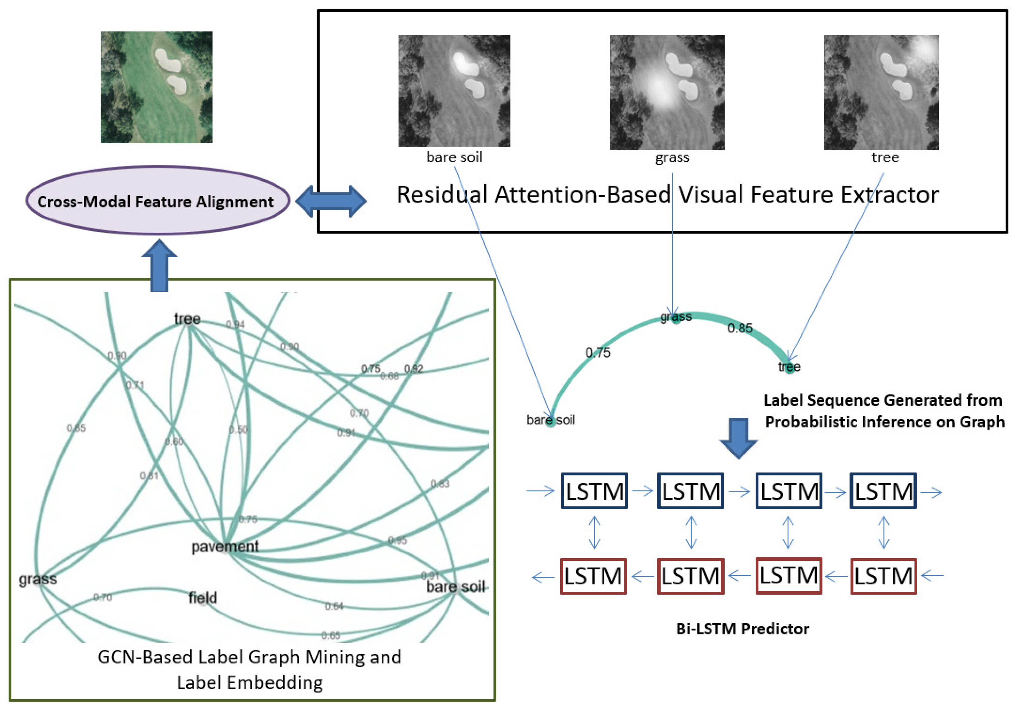
In the framework above, the object-level visual features would be extracted by the improved channel-wise multi-attentional CNN and then aligned to label vectors. After cross-modal mapping, we feed those object-level signals to a Bi-LSTM [19] predictor according to a label sequence that is generated by the probabilistic inference on label graph. The framework will be presented in detail in the following sections.

3.1. Residual Multi-Attention Mechanism

In this article, we introduce the advanced attention mechanism, MA-CNN [20], and further improve it for multi-label tasks. MA-CNN is proposed for fine-grained image categorization. For all training samples, the coordinates of peak response in each CNN layer are selected as the feature vector. With these vectors, CNN layers can be clustered into N groups, generating related discriminative attention parts. This is understandable, since the region with the peak response is always the most distinctive. This grouping operation is executed for the initialization of N attention parts. Correspondingly, N c-dimensional fully connected layers are designed to generate the weights of different channels (c channels) for these N attention parts. The fully connected layers will be optimized during the further end-to-end part learning. More details are described in reference [20].

Due to the fact that MA-CNN is proposed for fine-grained categorization for which the label for each sample is only one, we further improve MA-CNN in three aspects so as to make it appropriate for multi-label classification.

Firstly, the attention parts in MA-CNN [20] are proposed adaptively according to related labels. It is possible that more than one attention part is associated with the same tag. We utilize a pre-trained CNN to predict the labels for different attention parts. The part with the higher response value will be selected, as written in Equation (1):

$$Y_n=\mathit{V}\left({\mathit{P}}_{\mathit{n}}\left(\mathit{X}\right)\right)=\mathit{V}(\sum _{j=1}^c({[{\mathit{W}}_1\ast \mathit{X}]}_j·{\mathit{M}}_{\mathit{n}})),$$

(1)

where $Y_n$ is the predicted label for the No.n attention part ${\mathit{M}}_{\mathit{n}}$; ${\mathit{P}}_{\mathit{n}}$ is the final feature representation of this attention part; $\mathit{V}$ is the pre-trained CNN predictor; c is the number of channels; ${\mathit{W}}_1$ denotes the CNN parameters for the feature extraction and attention proposal; the dot product means element-wise multiplication; $\mathit{X}$ denotes the input samples; and ∗ means the convolutional and attention-proposal operation.

Secondly, because of the above, the attention proposal in MA-CNN is implemented by channel grouping; the channels in the CNN kernels always distribute unevenly in different groups. This can be improved by channel-wise normalization, as written in Equation (2):

$${\mathit{P}}_{\mathit{n}}\left(\mathit{X}\right)=\frac{1}{\left({\displaystyle \sum _{j=1}^c}{d}_j\right)}\sum _{j=1}^c(d_j{[{\mathit{W}}_1\ast \mathit{X}]}_j·{\mathit{M}}_{\mathit{n}}),$$

(2)

where ${\mathit{P}}_{\mathit{n}}\left(\mathit{X}\right)$ denotes the extracted feature associated with No.n attention mask, ${\mathit{M}}_{\mathit{n}}$; $d_j$ is one of the weights of the CNN channels generated from the fully-connected layers in MA-CNN; ${\mathit{W}}_1$ denotes the trainable CNN parameters; and the dot product means element-wise multiplication.

In addition, we introduce the residual attentional learning [41] in different channel groups, mining the residual, channel-wise, and regional information not only in depth but also crosswise, as in Equation (3):

$${\mathit{P}}_{\mathit{n}}\left(\mathit{X}\right)=\frac{1}{\left({\displaystyle \sum _{j=1}^c}{d}_j\right)}\sum _{j=1}^c(d_j{[{\mathit{W}}_1\ast \mathit{X}]}_j·\left(1+{\mathit{M}}_n\right)).$$

(3)

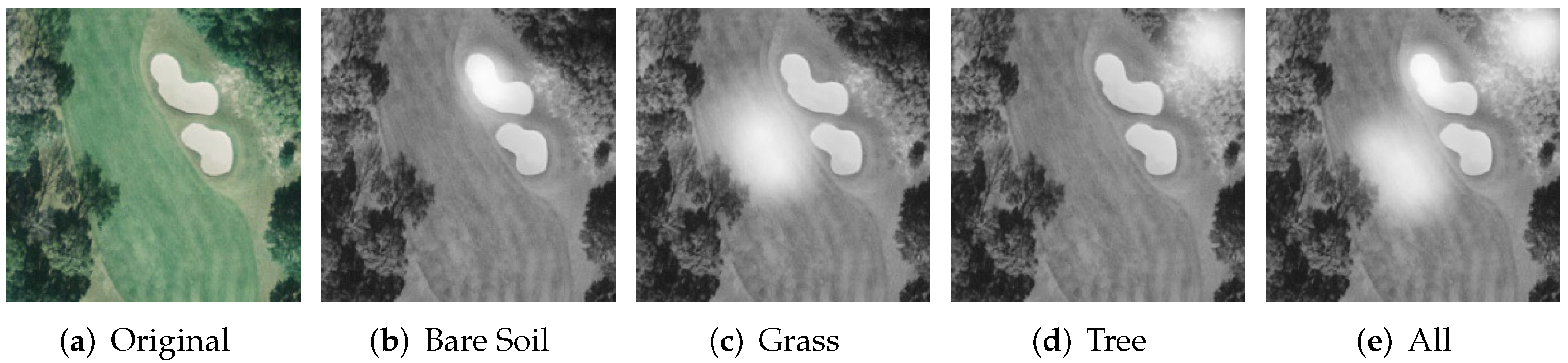
This residual, multi-attention mechanism (RMAM) is suitable for the analysis of complex remote sensing pictures with many labels. We visualize the generated attention parts in the picture “golfcourse79” (UC-Merced [16,17]) using the basic attention layer, MA-CNN, and the proposed RMAM, as in Figure 4. In these experiments, ResNet-50 [5] is selected as the backbone.

As illustrated in Figure 4, MA-CNN is more sensitive for object-level features than the basic attention layer. The perceived attention parts by our RMAN are most obvious, especially for label “tree” and the label “grass”.

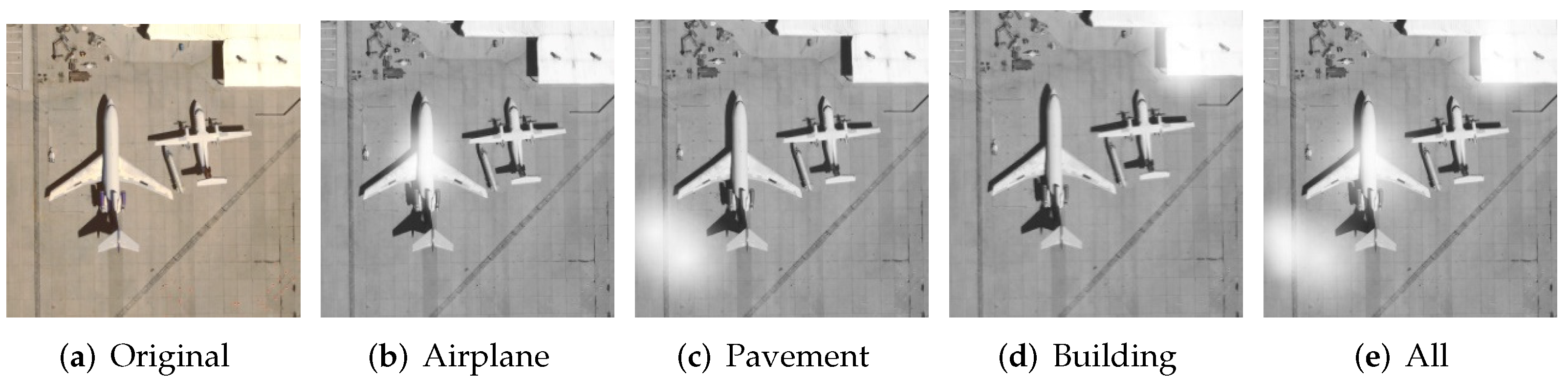
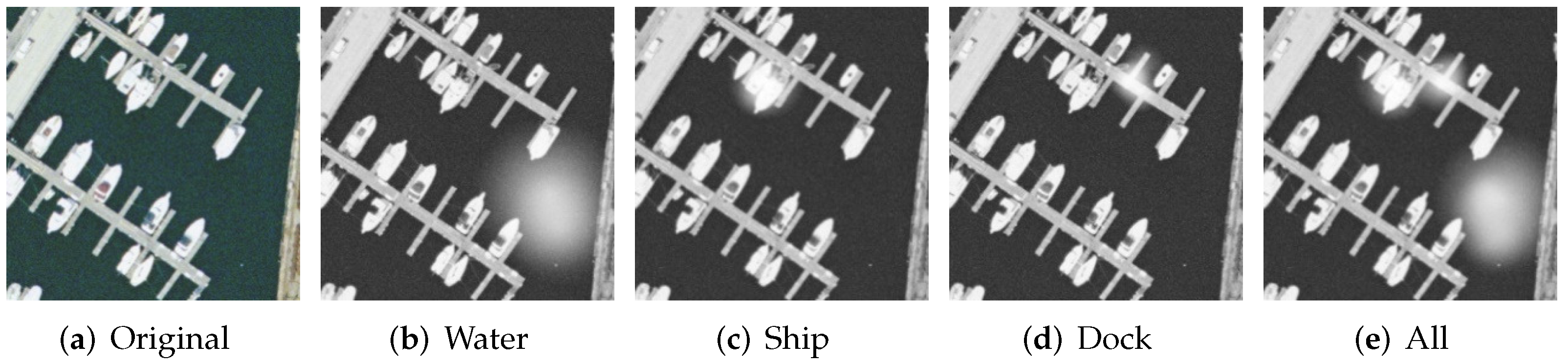
Figure 5, Figure 6 and Figure 7 show the generated attention parts associated with different labels by RMAN on three typical pictures. It is evident that RMAM is able to perceive object-level visual features effectively.

These extracted object-level visual signals will be further processed and then utilized for a sequence prediction which will be described in Section 3.3 and Section 3.4.

3.2. GCN-Based Label Representation Learning

As mentioned in Section 1 the most important issue in multi-label classification is to match visual features to semantic labels. If we pay more attention to label representation, multi-label classification can be regarded as a typical cross-modal learning process which tries to translate the high-level semantic concepts in pictures to a group of words. In this paper, we adopt a language model and label a graph to represent the labels, then map them to visual features. The mapping strategy will be described in Section 3.3.

Over the past few years, with the development of multi-media techniques, the data resource in the new period is characterized as multi-source and heterogeneous but highly correlated with high-level semantics [56]. Multi-modal machine learning has become a research hotpot in the past few years. As defined by [57], “modality” has a more fine-grained meaning compared with “medium”. It refers to a typical data source with a standard structure in a unified channel. On this precondition, pictures, texts, vocal signals, time series, or graphs can all be regarded as independent modes, respectively.

Textual data present valuable cross-modal supplementary information for the comprehension of label semantics. On a large scale corpus, images and texts, similar concepts (objects in pictures and entities in sentences), will always co-occur in specialized scenes. Most word-representation models are based on word distribution, e.g., close prediction in sentences, which is similar to object co-occurrence in pictures. In this article, in addition to mapping remote sensing images by CNN with residual multi-attention module (RMAM in Section 3.1 with attention masks optimized in the training process for associated labels), we also adopt an advanced language model, Bert [58], to initialize label representation with a large textual corpus.

Language model-based label representation is effective due to the fact that related entities always co-occur in large scale textual corpora. From another perspective, the large-scale data will also dilute the valuable information among specific words about the multi-label dataset. In order to ensure the good use of label dependencies, we further exploit them in a graph which is mined by GCN [18]. This is the so-called “label graph mining”-based label (node in graph), which embeds strategy in the proposed framework.

To begin, we built the label graph referred to as labels’ co-occurrence conditional probabilities, as Equation (4):

$$P\left(L_b\right|L_a)=\frac{P(L_a,L_b)}{P\left(L_a\right)},$$

(4)

where $L_a$ and $L_b$ denote label a and label b. If $P\left(L_b\right|L_a)$ is greater than a threshold (in this article, we set it 0.4), we consider that if $L_a$ appears, $L_b$ will also appear. The connection from $L_a$ to $L_b$ exists in the graph (such as in Figure 1).

Through the statistical analysis of training data, we can obtain a label graph. This graph can further be modeled by GCN [18]. The function for one GCN layer can be written in Equation (5):

$${\mathit{H}}^{l+1}=\sigma ({\tilde{\mathit{D}}}^{-\frac{1}{2}}\tilde{\mathit{A}}{\tilde{\mathit{D}}}^{-\frac{1}{2}}{\mathit{H}}^l{\mathit{W}}_G^l),$$

(5)

where ${\mathit{H}}^l$ is the result of the convolutional operation in No.l GCN layer; $\tilde{\mathit{A}}=\mathit{A}+{\mathit{I}}_N$ is the adjacency matrix of the graph; ${\mathit{H}}^0$ is initialized by a matrix of node feature vectors $X_i$; $\widetilde{D_{ii}}={\displaystyle \sum _j}{\tilde{A}}_{ij}$, where the introduction of $\tilde{\mathit{D}}$ is to normalize adjacency matrix; ${\mathit{W}}_G$ is a matrix of trainable variables in GCN; and $\sigma (·)$ is an nonlinear activation function, such as ReLU [59].

As mentioned above, we employ a language model to extract semantics in a textual corpus cross-modally, leveraging Bert [58] to embed labels initially. These label vectors will form the initial states (nodes) of the graph, also the $X_i$ and ${\mathit{H}}^{\mathit{0}}$ in Equation (5). Our CM-GM framework can not only extract word semantics in large corpus, but also take advantage of label dependencies by label graph mining.

It can be seen in Figure 8, compared with initial label vectors by Bert in Figure 8d, that further GCN mapping can make the related labels in one typical scene appear closer to each other, as shown in Figure 8e. In these experiments, we chose a pre-trained Bert model [58]. The dimension of the label vectors were set to 1000. t-SNE [60] is employed to reduce the dimensions of the label vectors for visualization.

3.3. Cross-Modal Feature Alignment and Training Approach

For multi-label classification and other multi-modal learning tasks, cross-modal feature alignment is a key point. With those visual embeddings (such as attentional feature vectors in Figure 5, Figure 6 and Figure 7) and graph-based label embeddings (such as in Figure 8), it is an important issue to align feature representations between 2 modes. In this article, we proposed an improved cross-modal representation learning strategy to enhance features in the framework cross-modally. That is minimizing hinge rank loss [61] to optimize the CNN layer, as Equation (6):

$$L_{\mathrm{cross}}=\sum _{a\ne label}max[0,\mathrm{margin}-{\mathit{g}}_{label}{\mathit{W}}_2{\mathit{P}}_{label}+{\mathit{g}}_a{\mathit{W}}_2{\mathit{P}}_{label}],$$

(6)

where ${\mathit{P}}_{label}$ is a column vector generated from object-level attention mechanism as mentioned in Section 3.1; ${\mathit{g}}_{label}$ denotes the label embedding, a row vector, of the matched label; $g_a$ are those embeddings of other labels (nodes) in the graph; and ${\mathit{W}}_2$ are trainable parameters in Cross Modal Alignment module (CMA).

${\mathit{P}}_{\mathit{label}}$, ${\mathit{g}}_{label}$ and ${\mathit{g}}_a$ can be calculated as Equations (7)–(9),

$${\mathit{P}}_{\mathit{label}}=RMAM\left(\mathit{X}\right),$$

(7)

$${\mathit{g}}_{label}=GCN\left({\mathit{L}}_i\right),$$

(8)

$${\mathit{g}}_a=GCN\left({\mathit{L}}_a\right),a\ne i,$$

(9)

where $\mathit{X}$ is the input sample, and ${\mathit{L}}_i$ is the label vector generated by Bert [58], and this label is associated with ${\mathit{P}}_{\mathit{label}}$.

In Figure 9, we visualize the extracted label–level feature vectors from three typical pictures. The vectors in Figure 9d are generated by RMAM, as mentioned in Section 3.1. After cross-modal feature alignment, visual vectors in the same scene become closer to each other and farther from those in other pictures, as shown in Figure 9e. Similarly, we use t-SNE [60] for dimensionality reduction. In fact, it has been analyzed that related objects and attributes are always distributed similarly in large corpora of different modes, and this data character is useful. This cross-modal similarity has been utilized in many complex computer vision tasks, e.g., zero-shot image classification based on semantic embedding [61,62].

In the training, we preserve two groups of trainable CNN parameters in the CM-GM framework, ${\mathit{W}}_1$ and ${\mathit{W}}_2$, for attention propose and cross-modal alignment, respectively. ${\mathit{W}}_1$ is to be used for the object-level visual feature extraction in RMAM, as mentioned in Section 3.1. ResNet-50 [5] is selected as the backbone. We use a similar training strategy for ${\mathit{W}}_1$ to MA-CNN, with the accumulation of binary cross-entropy loss and channel-grouping loss [20]. ${\mathit{W}}_1$ and the fully connected layer (FC layer) designed in the original MA-CNN can help our CM-GM framework to generate appropriate attention parts for different labels. With these attention parts, object (label)-level visual signals can be extracted one by one and aligned with associated label vectors by another CNN-based mapping with ${\mathit{W}}_2$, as written in Equation (6). The training processes for ${\mathit{W}}_1$, ${\mathit{W}}_2$ and the fully-connected layer (FC layer) for channel grouping in MA-CNN are individual and alternative. It can be summarized as follows:

• Train ${\mathit{W}}_1$ with fixed FC layer;
• Train FC layer with fixed ${\mathit{W}}_1$ generated in step 1;
• Train ${\mathit{W}}_2$ with attention parts generated by fixed ${\mathit{W}}_1$ and FC layer (updated in this loop); go to step 1 (next loop): train ${\mathit{W}}_1$ with the fixed and updated FC layer generated in this loop.

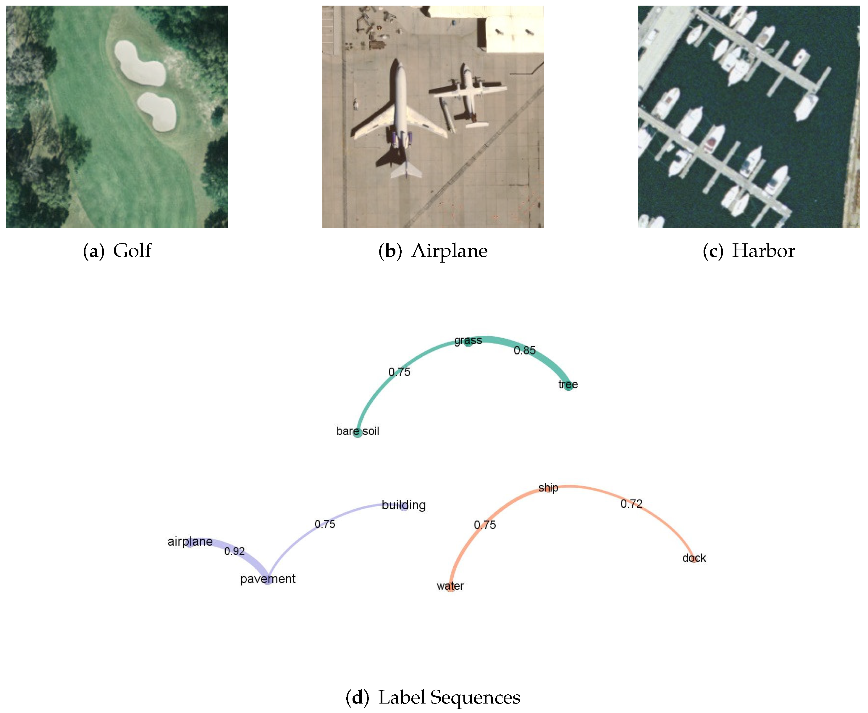
3.4. Credible Labels for LSTM Predictor

After being aligned and enhanced by a cross-modal alignment module, those object-level visual features would be fed into a LSTM [19] predictor for training and testing. In this paper, we model the label dependencies by GCN-based graph. After graph mining and embedding, we deal with these label (object)-level visual representations as a sequence generated from the graph (such as in Figure 1) by probabilistic inference. For example, the most obvious object, also the one with the peak response value, e.g., the “airplane” in Figure 10b, can be regarded as the starting point of the sequence. Another object with the highest co-occurrence probability is sequentially selected as the second one. Since $P\left(\mathrm{pavement}\right|\mathrm{airplane})>P(\mathrm{building}\left|\mathrm{airplane}\right)$, the label sequence in Figure 10b for LSTM can be determined like the purple curve in Figure 10d. Similarly, the label sequences for Figure 10a,c are also built and shown in Figure 10d. These three paths are cut from the label graph in Figure 1.

In the training process, we feed those mapped visual feature vectors (generated from the residual attentional CNN and aligned by cross-modal module) to the LSTM [19,44] predictor. Compared to the classical RNN, LSTM is more applicable for a sequence process with a higher memory ability. In LSTM, different memory units and gates are designed. Their updating formula is written in Equations (10)–(14):

$${\mathit{i}}_n=\sigma ({\mathit{W}}_{pi}{\mathit{P}}_n^{\prime }+{\mathit{W}}_{hi}{\mathit{h}}_{n-1}+{\mathit{W}}_{ci}{\mathit{c}}_{n-1}+{\mathit{b}}_i),$$

(10)

$${\mathit{f}}_n=\sigma ({\mathit{W}}_{pf}{\mathit{P}}_n^{\prime }+{\mathit{W}}_{hf}{\mathit{h}}_{n-1}+{\mathit{W}}_{cf}{\mathit{c}}_{n-1}+{\mathit{b}}_f),$$

(11)

$${\mathit{o}}_n=\sigma ({\mathit{W}}_{po}{\mathit{P}}_{\mathit{n}}^{{}^{\prime }}+{\mathit{W}}_{ho}{\mathit{h}}_{n-1}+{\mathit{W}}_{co}{\mathit{c}}_n+{\mathit{b}}_f),$$

(12)

$${\mathit{c}}_n={\mathit{f}}_n•{\mathit{c}}_{n-1}+{\mathit{i}}_n•tanh({\mathit{W}}_{pc}{\mathit{P}}_n^{\prime }+{\mathit{W}}_{hc}{\mathit{h}}_{n-1}+{\mathit{b}}_c),$$

(13)

$${\mathit{h}}_n={\mathit{o}}_{n}tanh\left({\mathit{c}}_n\right),$$

(14)

where, ${\mathit{i}}_n$, ${\mathit{f}}_n$, and ${\mathit{o}}_n$ denote the outputs of “input gate”, “forgetting gate”, and “output gate” at time t, respectively (in this paper, these outputs are calculated for the nth label; one label corresponds to one step); ${\mathit{c}}_n$ means the state of the LSTM [19] cell; ${\mathit{h}}_n$ is the hidden variable of the LSTM cell, the activation of ${\mathit{c}}_n$; $\mathit{W}$ denotes trainable variables in different units, and $\mathit{b}$ is the corresponding bias; ${\mathit{P}}_n^{\prime }$ is the visual feature vector of attention part n as Equation (15), related with label n; $\sigma$ is a nonlinear activation function, “sigmod”, in LSTM; and • denotes element-wise multiplication.

$${\mathit{P}}_{\mathit{n}}^{{}^{\prime }}=CMA\left(RMA{M}_n\left({\mathit{X}}_{\mathit{k}}\right)\right)=CMA\left({\mathit{P}}_{\mathit{n}}\left({\mathit{X}}_{\mathit{k}}\right)\right),$$

(15)

where $CMA$ denotes cross modal alignment; we let ${\mathit{X}}_{\mathit{k}}$ be the No. k sample and ${\mathit{P}}_{\mathit{n}}$ be the visual features generated by RMAM associated with No. n label in sample k.

Considering the rich information in the sequence and the differences in label directions (For 2 labels, A and B, it is normal that $P\left(\mathrm{A}\right|\mathrm{B})\ne P(\mathrm{B}\left|\mathrm{A}\right)$), we improve the LSTM to Bi-directional LSTM as Equation (16):

$$\overleftrightarrow{{\mathit{h}}_n}=\overrightarrow{[{\mathit{h}}_n};\overleftarrow{{\mathit{h}}_n}],$$

(16)

where $\overleftrightarrow{{\mathit{h}}_n}$ denotes the final hidden variable, which is the concatenation of ${\mathit{h}}_n$ in two opposite directions, $\overrightarrow{\mathit{h}{}_n}$ and $\overleftarrow{\mathit{h}{}_n}$.

In the testing, we consider the labels with higher CNN output values (top K or bigger than a threshold) as “credible labels”, then predict the last labels in the sequence by LSTM [19]. With these output vectors of LSTM, label vectors can be determined by mapping or inverse mapping, as mentioned in Section 3.2.

We adopt a pre-trained CNN classifier (e.g., ResNet [5] on MS-COCO or the large remote sensing archive) to predict labels. If the predicted labels (not in a credible label set) are also in the predictions of LSTM, we consider these predicted labels to also be positive. Our experiments show that this LSTM predictor is very effective. This is understandable, since the prediction about obvious objects is more likely to be correct in a multi-label classification. For those inconspicuous objects, the CM-GM framework is also valid due to its advantage in graph mining and sequence analysis.

Moreover, considering the the co-occurrence of related labels and the actual situation that some of the objects are obvious in one picture while inconspicuous in another one, it is reasonable to believe that we can utilize partially significant objects to illustrate a special scene in a large image archive on the condition that the labels are jointly represented by the graph cross-modally. In this way, the manual labeling work for training data can be reduced significantly.

4. Experiments

4.1. Implementation Details

4.1.1. Baselines and Metrics

To evaluate the performance of the proposed CM-GM framework in this paper, we carried out experiments compared with several popular multi-label classification algorithms. They are: ResNet-RBFNN [63], CA-ResNet-LSTM [44], CNN-RNN [14], WAPR [64], LSEP [65], and ML-GCN [15]. Among these methods, ResNet-RBFNN [63] and CA-ResNet-LSTM [44] are proposed for aerial images; CNN-RNN [14], WAPR [64], LSEP [65], and ML-GCN [15] are state-of-the-art in general multi-label image recognition tasks. We substitute ResNet [5] for GoogLeNet in original GoogLeNet-RBFNN [63] in order to make a fair comparison, similar to [44].

For multi-label evaluation, we adopt six metrics: Overall Precision (OP), Overall Recall (OR), Per-Class Precision (CP), Per-Class Recall (CR), Micro F1 (MiF1), and Macro F1 (MaF1). They can be calculated using Equations (17)–(22):

$$OP=\frac{{\displaystyle \sum _{i=1}^c}{N}_i^a}{{\displaystyle \sum _{i=1}^c}{N}_i^p},$$

(17)

where $N_i^a$ is the number of samples predicted to be associated with the ith label, and the actual number is i; $N_i^p$ denotes all the samples predicted to the ith label;and c is the number of labels.

$$OR=\frac{{\displaystyle \sum _{i=1}^c}{N}_i^a}{{\displaystyle \sum _{i=1}^c}{N}_i^g},$$

(18)

where $N_i^g$ is the number of samples with No.i label in the whole dataset.

$$CP=\frac{1}{c}{\displaystyle \sum _{i=1}^c}\frac{N_i^a}{N_i^p},$$

(19)

$$CR=\frac{1}{c}{\displaystyle \sum _{i=1}^c}\frac{N_i^a}{N_i^g},$$

(20)

$$MiF1=\frac{2OP\times OR}{OP+OR},$$

(21)

$$MaF1=\frac{2CP\times CR}{CP+CR}.$$

(22)

4.1.2. Experimental Platform and Hyper Parameters

In this article, all the experiments are carried out on a workstation with two Intel Xeon(R) E5-2640K CPUs @2.4GHz, one 64GB RAM, and two 11GB GeForce RTX 2080 Ti GPUs. The Integrated Development Environment (IDE) is Pycharm on Ubuntu 18.04.1. In addition, we adopt TensorFlow1.12 as a deep learning framework. ResNet-50 and ResNet-101 [5] are our backbones.

We train the feature extractor using a stochastic gradient descent optimizer with a batch size of 50, momentum of 0.9, and weight decay of 0.0001. The learning rate is initialized as 0.0001 and divided by 10 every epoch until the validation performance converges. Then, we freeze the weights of all the convolution layers in the backbone network and train the multi-label reasoning module using an Adam optimizer. The early stopping strategy is adapted to figure out the appropriate training epoch. The hidden size in LSTM [19] is set to 512, and the embedding size is also 512. Moreover, $batch$ $normalization$ is also utilized. In our experiments, the labels with higher CNN output values (bigger than 0.4) are set as credible labels.

4.1.3. Training and Testing Details

For those CNN parameters in the visual feature extractor, ${\mathit{W}}_1$ in RMAM, cross-modal alignment mapping, and ${\mathit{W}}_2$ in CMA, we train them alternatively as mentioned in Section 3.3. For the graph-based label representation mapping, ${\mathit{W}}_G$, we train them as general GCN [18]. The object-level visual feature vectors would be fed into the LSTM [19], following the sequences mentioned in Section 3.4, thus training the LSTM predictor by cross-entropy loss.

We use pre-trained Bert [58] with 1000-Dimensional vectors for the first-step label representation and t-SNE [60] to reduce the dimension for visualization.

In testing, the pictures are firstly perceived by trained RMAM. With these mapped visual signals, the pre-trained CNN is able to make initial predictions. We align the visual signals associated with the top K labels to the GCN-based label embeddings by CMA, then feed them to LSTM for a complete sequence. If the initially predicted labels are also in this sequence, we consider this label to be positive.

4.2. Experiments on UC-Merced

The UC-Merced land use dataset is our first benchmark, which was initially proposed by Yang et al. in a single-label style [16]. Chaudhuri et al. reproduced this dataset by labeling multiple different objects in the pictures [17]. UC-Merced is a classical and popular dataset for evaluating different models in remote sensing image processing. The number of images associated with each class label in UC-Merced is shown in

Table A1. Number of images associated with each class label in UC-Merced archive.

Class Label	Number of Images
airplane	100
bare soil	633
building	696
car	884
chaparral	119
court	105
dock	100
field	106
grass	977
mobile home	102
pavement	1305
sand	389
sea	100
ship	102
tanks	100
trees	1015
water	203

.

In the tables below, “N” denotes channel-wise normalization, and “R” denotes residual attentional learning, respectively. As listed in

Table 1. The performance of different models on UC-Merced multi-label dataset.

Model	MiF1	MaF1	OP	OR	CP	CR
ResNet-50 [5]	79.51	80.41	80.70	81.97	88.52	78.91
ResNet-RBFNN [63]	80.58	82.47	79.92	84.59	86.21	83.72
CA-ResNet-LSTM [44]	81.36	83.66	79.90	86.14	86.99	82.24
CA-ResNet-BiLSTM [44]	81.47	85.27	77.94	89.02	86.12	84.26
CM-GM-N-LSTM	79.56	84.22	78.17	87.56	87.28	83.51
CM-GM-N-R-LSTM	81.31	85.52	81.20	89.41	88.35	85.06
CM-GM-N-BiLSTM	81.21	85.42	81.12	89.23	88.17	84.85
CM-GM-N-R-BiLSTM	81.58	86.19	81.6	89.65	88.57	85.20

, it is obvious that the performance of the basic feature extractor, ResNet-50, is weaker than other models. Although its $CP$ is acceptable, the $CR$ is the lowest among the models. The introduction of the RBF network helps the model, ResNet-RBFNN [63], perform better in almost all the indicators, except $OP$ and $CP$, than ResNet-50 [5]. CA-ResNet-LSTM [44] obtained better MiF1 and MaF1 values. This illustrates that the sequence-based classification is superior than those soft-max-based methods in our experiments. BiLSTM can further improve the model’s capabilities. For our CM-GM framework, it can be seen that, along with the development of the attention mechanism, all the indicators increase gradually. With the improvements in RMAM, the residual mechanism, and channel-wise normalization, our CM-GM-BiLSTM framework outperforms all the other methods. The proposed object-level attention mechanism and the cross modal alignment strategy are effective.

Figure 11 shows the average precision–recall curves of the different models on the UC-Merced dataset. It can be seen that the performance of ResNet-RBFNN [63] is slightly superior to that of basic ResNet-50 [5]. Our CM-GM performs better than CA-ResNet-BiLSTM [44] and ResNet-RBFNN [63]. The curve of CM-GM is smoother and has a bigger area above the horizontal axis.

4.3. Experiments on BigEarthNet

The BigEarthNet [66] dataset originates from the Technische Universitaet Berlin, 2019. To our knowledge, BigEarthNet is the most comprehensive and largest remote sensing image archive at present. It contains 590,326 pictures from the Sentinel-2 satellite, associated with 43 categories. In this article, we only adopt R/G/B, three visible light bands. The number of images associated with each land-cover class in BigEarthNet is shown in

Table A2. Number of images associated with each land-cover class in BigEarthNet.

Class Label	Number of Images
Mixed forest	217,119
Coniferous forest	211,703
Non-irrigated arable land	196,695
Transitional woodland/shrub	173,506
Broad-leaved forest	50,944
Land principally occupied by agriculture, with significant areas of natural vegetation	147,095
Complex cultivation patterns	107,786
Pastures	103,554
Water bodies	83,811
Sea and ocean	81,612
Discontinuous urban fabric	69,872
Agro-forestry areas	30,674
Peatbogs	23,207
Permanently irrigated land	13,589
Industrial or commercial units	12,895
Natural grassland	12,835
Olive groves	12,538
Sclerophyllous vegetation	11,241
Continuous urban fabric	10,784
Water courses	10,572
Vineyards	9567
Annual crops associated with permanent crops	7022
Inland marshes	6236
Moors and heathland	5890
Sport and leisure facilities	5353
Fruit trees and berry plantations	4754
Mineral extraction sites	4618
Rice fields	3793
Road and rail networks and associated land	3384
Bare rock	3277
Green urban areas	1786
Beaches, dunes, sands	1578
Sparsely vegetated areas	1563
Salt marshes	1562
Coastal lagoons	1498
Construction sites	1174
Estuaries	1086
Intertidal flats	1003
Airports	979
Dump sites	959
Port areas	509
Salines	424
Burnt areas	328

. ResNet-50 [5] is selected as the backbone. A total of 60% of samples are used for training, and the rest is used for testing.

The performance of the different models on BigEarthNet [66] is shown in

Table 2. The performance of different models on BigEarthNet.

Model	MiF1	MaF1	OP	OR	CP	CR
ResNet-50 [5]	81.56	80.53	81.22	82.32	89.12	79.23
ResNet-RBFNN [63]	82.72	83.51	80.25	84.83	86.51	83.96
CA-ResNet-LSTM [44]	83.35	84.96	80.18	86.68	87.30	82.63
CA-ResNet-BiLSTM [44]	84.50	85.61	78.37	89.41	86.69	84.67
CM-GM-N-LSTM	84.36	85.31	78.71	87.89	87.63	83.82
CM-GM-N-R-LSTM	85.32	86.26	81.53	89.92	88.72	85.66
CM-GM-N-BiLSTM	85.23	86.61	81.61	89.87	88.65	85.34
CM-GM-N-R-BiLSTM	85.52	86.82	81.76	89.96	88.80	85.91

. The introduction of channel-wise normalization and residual attentional learning can improve CM-GM effectively. As a result, GM-GM gains excellent performance on almost all the indicators, about 1% higher than the state-of-the-art method CA-ResNet-BiLSTM [44] on MiF1 and MaF1.

The average precision–recall curves on BigEarthNet are shown in Figure 12. The curve obtained by CM-GM is better than other models, with the biggest area under the curve. The curve of CA-ResNet-BiLSTM [44] is near to and better than ResNet-RBFNN [63]. By contrast, the baseline, ResNet-50 [5], is weaker.

4.4. Additional Experiments on MS-COCO

We also conduct addition experiments on the popular computer vision benchmark dataset, MS-COCO [67], only with object-level labels (without bounding boxes and pixel-level labels). As was the case in [65], there are 82,081 training samples and 40,137 testing samples. The number of images associated with each class label in MS-COCO is shown in

Table A3. Number of images associated with each class label in MS-COCO.

Class Label	Number of Images
person	64,115
bicycle	3252
car	12,251
motorcycle	3502
airplane	2986
bus	2952
train	3588
truck	6127
boat	3025
traffic light	4139
fire hydrant	1711
stop sign	1734
parking meter	705
bench	5570
bird	3237
cat	4114
dog	4385
horse	2941
sheep	1529
cow	1968
elephant	2143
bear	960
zebra	1916
giraffe	2546
backpack	5528
umbrella	3968
handbag	6841
tie	3810
suitcase	2402
frisbee	2184
skis	3082
snowboard	1654
sports ball	4262
kite	2261
baseball bat	2506
baseball glove	2629
skateboard	3476
surfboard	3486
tennis racket	3394
bottle	8501
wine glass	2533
cup	9189
fork	3555
knife	4326
spoon	3529
bowl	7111
banana	2243
apple	1586
sandwich	2365
orange	1699
broccoli	1939
carrot	24
hot dog	11
pizza	3166
donut	1523
cake	2925
chair	12,774
couch	4423
potted plant	4452
bed	3682
dining table	11,837
toilet	3353
tv	4561
laptop	3524
mouse	1876
remote	3076
keyboard	2115
cell phone	4803
microwave	1547
oven	2877
toaster	217
sink	4678
refrigerator	2360
book	5332
clock	4659
vase	3593
scissors	947
teddy bear	16
hair drier	189
toothbrush	1007

. In these experiments, ResNet-101 [5] is selected as the backbone, different from the original backbones adopted by the methods for comparison, such as VGG16 [34] in CNN-RNN [14] and LSEP [65]. The results are recorded in

Table 3. The performance of different models on MS-COCO.

Model	MiF1	MaF1	OP	OR	CP	CR
ResNet-101 [5]	76.8	72.9	83.7	71.0	80.4	66.9
WARP [64]	77.0	74.1	83.9	71.3	81.2	68.2
LSEP [65]	78.7	75.6	84.6	73.5	83.4	69.1
CNN-RNN [14]	78.1	74.3	84.2	72.9	82.7	67.5
ML-GCN [15]	81.1	78.7	86.5	76.3	85.7	72.8
CM-GM-N-LSTM	79.3	77.3	84.5	74.7	84.3	71.3
CM-GM-N-R-LSTM	79.9	77.9	85.3	75.3	85.5	71.6
CM-GM-N-BiLSTM	81.0	78.8	86.2	76.4	86.3	72.5
CM-GM-N-R-BiLSTM	81.9	79.6	87.1	77.2	87.1	73.3

.

As listed in Table 3, the basic feature-extraction network ResNet-101 [5] has a weaker performance on multi-label indicators. Compared with ResNet-101 [5], the methods with improved losses, such as WARP [64] and LSEP [65], perform better. LSEP [65] outperforms CNN-RNN [14] on almost all the indicators. In ML-GCN [15] and CM-GM, label graphs are used to improve the models. Along with different improvements, such as channel-wise normalization and residual attentional learning utilized in CM-GM, our framework has the best performance on all indicators.

It can be seen in Figure 13 that the average precision–recall curve obtained by CM-GM has the biggest area under the curve. In the part with higher recalls, ML-GCN [15] and LSEP [65] can also achieve higher accuracy.

4.5. Ablation Study and Qualitative Analysis

In the experiments mentioned above, the proposed CM-GM framework is fixed. In addition, those statistical results about CM-GM can illustrate the effects of the feature extractor RMAN, as mentioned in Section 3.1, including channel-wise normalization and residual attentional learning. In this section, we mainly focus on the ablation studies about different sub-modules, e.g., GCN-based label graph mining and cross-modal alignment. MS-COCO [67] is selected as the benchmark for its representativeness.

We initially classify those object-level visual representations before and after cross-modal alignment by a ResNet-50 [5] classifier pre-trained on ImageNet [6]. The results (MiF1/MaF1) are listed in

Table 4. MiF1/MaF1 by ResNet-50 on MS-COCO (before and after alignment).

Before Alignment	71.1/67.6
After Alignment	Aligned by Bert	Aligned by GCN
	73.6/70.5	76.2/74.1

. It can be seen that, after cross-modal feature alignment, the multi-label perceptual ability is enhanced. The alignment by GCN [18] can further embed labels according to their internal relationships, enabling the classifier to obtain higher MiF1/MaF1 values than the alignment by Bert [58].

Similarly, the LSTM [19] classifier is also applied to recognize those object-level visual signals obtained by RMAM and further aligned to different label embeddings. The results are listed in

Table 5. MiF1/MaF1 by LSTM on MS-COCO (before and after alignment).

Before Alignment	78.2/72.3
After Alignment	Aligned by Bert	Aligned by GCN
	78.5/74.6	79.9/77.9

. Compared with the results in Table 4, the LSTM classifier performs better. The GCN [18] alignment is superior to Bert [58]. This is because the sequence predictor is able to utilize more instruction information from the label graph.

Figure 14, Figure 15 and Figure 16 show the qualitative results about three pictures from MS-COCO. In these examples, green labels denote true positive, red labels denote false positive, and gray labels denote false negative.

In Figure 14, it can be seen that ResNet-101 [5] obtains a wrong prediction of “train”. This model is weaker at distinguishing easily confused visual features. For those inconspicuous objects such as “traffic light” and “truck”, CM-GM can also recognize them accurately, better than other methods.

In Figure 15, these models show similar performance. ResNet-101 [5] has a wrong prediction of “bottle”. CM-GM has a stronger ability to perceive inconspicuous objects such as “dining table” and “cup”. ML-GCN [15] also obtains better performance.

Figure 17, Figure 18 and Figure 19 are qualitative examples of the UC-Merced multi-label dataset. From the experimental results, we can easily find that Resnet-101 [5] tends to mis-detect some objects, such as the long-shaded part in Figure 17, which it classified as “water”. That is because the model only utilized pixel- or shape-based low-level features. CNN-RNN [14] can extract visual features by CNN and deal with label dependencies based on their frequencies of occurrence, so it obtains a lower false positive rate than ResNet-101 [5]. WARP [64] introduces a weighted approximate ranking strategy to optimize the accuracy of top-k labels, and LSEP [65] further improves the pair-wise loss and proposes a smooth approximation. As a result, these two methods have certain advantages in recognition accuracy. In addition, ML-GCN [15] models label dependencies as a directed graph and designs a novel graph convolutional network based on visual representation learning; therefore, the performance of ML-GCN [15] is superior to those models mentioned above. Due to the label-level channel-wise pooling and cross-modal feature alignment strategy, CM-GM has a better performance on both UC-Merced examples than ML-GCN [15].

It is obvious that the sequence-prediction method and cross-modal alignment make the proposed CM-GM more sensitive to those inconspicuous objects, such as the “car” in Figure 19, considering the related labels in semantic scenes.

5. Discussion

The CM-GM framework is effective in multi-label tasks since it introduces an object-level attention mechanism and a cross-modal learning strategy. The framework is different from other state-of-the-art frameworks.

Difference with CA-ResNet-LSTM CA-ResNet-LSTM [44] adopts a classical attention layer for object-level feature extraction. In the CM-GM framework, the visual attention mechanism is more complex. Channel grouping can obtain more well-directed, objective-level feature vectors. Moreover, cross-modal learning is introduced in the CM-GM framework, in which the textual corpus and label graph provide valuable information for feature representation. The cross-modal supplementary information is integrated and enhanced by a feature-alignment module in the CM-GM framework. In addition, we utilize probabilistic inference-based sequences for the LSTM predictor.

Difference with ML-GCN The visual representation learning in ML-GCN [15] is by general CNN architectures. Different from ML-GCN [15], the CM-GM framework employs an improved object-level feature extractor, RMAM, which can extract visual attention parts then connect them to associated labels initially. Both the CM-GM framework and ML-GCN [65] construct a label graph, then represent labels by GCN [18]. In ML-GCN [15], GCN-based label (node) representations were considered to be learned classifiers, which could be applied to image representations by dot product. The weights are trainable with classical binary cross-entropy loss. In the CM-GM framework, these label representations are used for the cross-modal alignment process. Aligned object-level visual features will be fed into a sub-module, the LSTM predictor, which is absent in ML-GCN [15].

It should be noticed that the alternative training in the CM-GM framework has brought more computational expense. The training time for UC-Merced is thirteen hours, and the time for MS-COCO is about 28 hours on our workstation, which is still acceptable. In addition, we believe that this can be solved by the development of hardware. In addition, our model relies on large-scale datasets to recognize the semantic context of a visual scene and the correlation of information between labels. However, acquiring massive labeled data is costly and difficult. Therefore, semi-supervised multi-label classification based on transfer learning is our future research topic.

6. Conclusions

Aerial scene classification is a fundamental and important problem, which can gain semantic information from images and directly impact the performance of subsequent computer vision tasks. In this article, we proposed a CM-GM framework for multi-label aerial scene classification. CM-GM can effectively extract object-level visual features by an improved residual multi-attention mechanism, which is helpful to reduce the error-detection rate of our model. In addition, the proposed method can also make good use of label dependencies. The label representation module in CM-GM is able not only to leverage textual data as valuable cross-modal information, but also to map the relevant objects into a graph semantically, utilizing the tacit knowledge between labels. With the improved sequence prediction sub-module, CM-GM has an advantage in the perception of inconspicuous objects, which can improve the recall rate significantly. Experimental results and qualitative analyses show that the proposed CM-GM achieves excellent performance on benchmark datasets when compared with state-of-the-art methods and is very suitable for multi-label classification in the remote sensing field.