Evaluating the Effectiveness of Machine Learning and Deep Learning Models Combined Time-Series Satellite Data for Multiple Crop Types Classification over a Large-Scale Region

Abstract

Accurate extraction of crop cultivated area and spatial distribution is essential for food security. Crop classification methods based on machine learning and deep learning and remotely sensed time-series data are widely utilized to detect crop planting area. However, few studies assess the effectiveness of machine learning and deep learning algorithm integrated time-series satellite data for identifying multiple crop type classification over a large-scale region. Hence, this study aims to evaluate the effectiveness of machine learning and deep learning models in crop classification and provide a framework for large-scale multiple crop type classification based on time-series of satellite data. The time-series of the Normalized Difference Vegetation Index (NDVI), Enhanced Vegetation Index (EVI), and NaE (combined NDVI and EVI) were adopted as input features, and four widely used machine learning models, including Support Vector Machine (SVM), Random Forest (RF), K-Nearest Neighbor (KNN), and their integration (Stacking) were compared to examine the performance of multiple crop types (i.e., wheat, corn, wheat-corn, early rice, and early rice-late rice) classification in the North China Plain. The performance of two types of deep learning classifiers: the One-dimensional Convolutional Neural Network (Conv1D) and Long Short-Term Memory Networks (LSTM), were also tested. The results showed that the NaE feature performed best among three input features, and the Stacking model produced the highest accuracy (77.12%) compared to other algorithms.

1. Introduction

Multi-temporal remote sensing (RS) data have been widely used for agricultural monitoring and crop identification studies [1,2,3,4], and these data provide the growth status of vegetation through time-series observations that can be used to identify types of vegetation coverage. In crop classification studies, a combination of optical and radar images is widely used to identify the type of crops [2,5,6], time-series data provide important information such as seasonal patterns and sequential relationships of crops. Therefore, more and more studies extract features from time-series to obtain useful information about crop growth status and crop planting type [7,8].

In recent years, some studies have utilized vegetation index (VI) time-series data from multi-temporal remote sensors to perform crop planting area recognition or vegetation classification [9,10,11]. A common approach to handling multi-temporal VI data is to retrieve temporal features or phenological metrics from time-series remotely sensed data [10]. Simple statistics or threshold-based methods used global statistics and selected appropriate threshold values to calculate phenological metrics, such as the maximum VI, the peak time of VI, start of the growing season, and end of the growing season, which will improve the ability to crop identification compared to the original VI data. [9,12]. Potgieter et al. [13] used multi-year MODIS data through a threshold-based classification method to estimate the total area of winter crops in two counties of Australia and achieved an accuracy of 94%. More sophisticated temporal feature extraction methods such as pre-defined mathematical formulas or models are also widely used in multi-temporal classification studies [14]. In these studies, time-series data were processed by a predefined function, such as weighted linear regression [15], asymmetric Gaussian smoothing [16,17], wavelet transform [14,18,19], a Savitzky–Golay filter [20,21], and Fourier transform [22,23]. Jönsson and Eklundh [16] adopted a nonlinear fitting method to smooth the Normalized Difference Vegetation Index (NDVI) data in Africa and derived the key seasonal parameters from the smoothed data. Shao et al. [20] smoothed MODIS NDVI time-series data using Savitzky–Golay, asymmetric Gaussian, and transformation algorithms to provide continuous phenology data for land cover classifications in the Laurentian Great Lakes Basin. This experiment indicated that applying a smoothing algorithm reduced image noise notably compared to the raw data.

Although the above approaches based on temporal feature extraction have demonstrated exemplary performance in crop classification, there have some flaws in practice. Generally, the commonly adopted methods such as threshold-based or simple statistics rely on the expert’s experience and domain knowledge; temporal feature extraction by human expert experience inevitably leads to data information loss or incomplete utilization. Therefore, these approaches lack full utilization of the temporal information in the time-series data, which would limit the effectiveness and reliability of feature extractors [24,25,26,27].

In order to make full use of the temporal features derived from time-series data, a suitable time-series feature extractor should be selected [4,28,29]. Ideally, a temporal feature extractor can be trained iteratively to automatically extract features from the data and applied to a series of crop planting classification studies. The active field of machine learning (ML) and deep learning (DL) provided solution approaches to this task. ML and DL can learn directly from the original values of RS data, which avoid data loss or incomplete utilization due to artificial influence and reduce the prior pre-processing process when extracting features based on time-series data [30,31]. In terms of ML, due to their advantages such as excellent generalization ability and suitability for tackling nonlinear issues, these algorithms such as Support Vector Machine (SVM), Random Forest (RF), K-Nearest Neighbor (KNN), are widely used in the studies of RS multi-temporal crop planting area identification [32,33]. Zhong et al. [34] adopted the crop phenology indicators derived from NDVI and a decision tree to classify crops in the San Joaquin Valley, California. Compared with traditional maximum likelihood classification methods, this phenology-based approach showed a higher classification accuracy. Lu et al. [35] utilized both image-based and pixel-based KNN algorithms combined with Landsat-8 images to classify land cover type in Zhongwei City of China; the results showed that the classification accuracy was above 90%. Furthermore, compared with the single classifier, the stacking multiple ML classifiers provides advantage for estimation crop classification [36,37]. Löw et al. [38] combined the SVM and RF models for multiple crop type mapping in regions of Uzbekistan by analyzing the multispectral images from the RapidEye system and achieved an accuracy of 94.6%. Yuan et al. [37] integrated multiple models (the Stacking algorithm), enabling a 6.78% accuracy improvement for rice classification compared with the single classifier. These results also indicated that integrating multiple classifiers for classification achieved more satisfying results than a single classifier. Besides ML, DL algorithms have also been gradually used for multi-temporal crop classification research. [29,30,39]. Compared with ML, DL does not require manual hyperparameters selected when extracting features and obtained satisfactory results for crop classification [8,25]. Ji et al. [30] adopted multi-temporal remote sensing images and Convolutional Neural Networks (CNN) to classify crops, which achieved an overall accuracy of 98.9%. Recurrent Neural Networks (RNNs) are mainly used to analyze RS images due to their ability to process the continuous dimensions data with sequential dependence [31]. As a particular type of RNN, LSTM could learn the long-term dependent information from time-series data [40]. The performance of the multiple variants of RNN was compared based on two datasets in Brazil, and the crop recognition results showed that the LSTM outperformed RNN [28].

In terms of ML and DL combined time-series satellite data for identifying the crop types, Rodriguez-Galiano et al. [41] extracted the phenological metrics from the time-series of Landsat-5 Thematic Mapper data and identified the 14 different land categories using the RF classifier in the south of Spain. Kumar et al. [27] concatenated multi-temporal scenes acquired by Landsat-8 and Sentinel-1A RS satellites and applied 1D convolution to the temporal domain for land cover classification in Ukraine. One of the advantages of ML and DL combined time-series data methods is that they do not require pre-processing of time-series curves and definition of functions. Another major application of this method is to evaluate the effectiveness of classifiers. Zhong et al. [25] designed two types of Deep Neural Network (DNN) models and reconstructed three widely used machine learning classifiers to extract features from EVI time series for multi-temporal crop classification in Yolo County, California, US. He et al. [24] employed A-LSTM networks to extract temporal features from MODIS time-series image observations and compared the performance with RF for winter wheat identification in Huanghuaihai Region. However, previous studies, such as those of He et al. [24], Tuanmu et al. [42], Zhong et al. [25], and others on crop classification or land cover identification were only conducted in a small area or classified only one crop type. Simultaneous experiments with large-scale regions and multiple crop types to assess the effectiveness of classifiers have attracted less attention. This study aims to assess the effectiveness of multiple ML and DL methods combined time-series satellite data to present multiple crop type classification over a large-scale region. Hence, the main objectives of this study are: (1) to combine six ML and DL algorithms and three remotely sensed time-series input features, (2) to explore the effectiveness of six training strategies in multiple crop type classification over large scale regions, (3) to compare the best-performing models among ML and DL approaches, and to evaluate the advantages and disadvantages of these models.

2. Materials and Methods

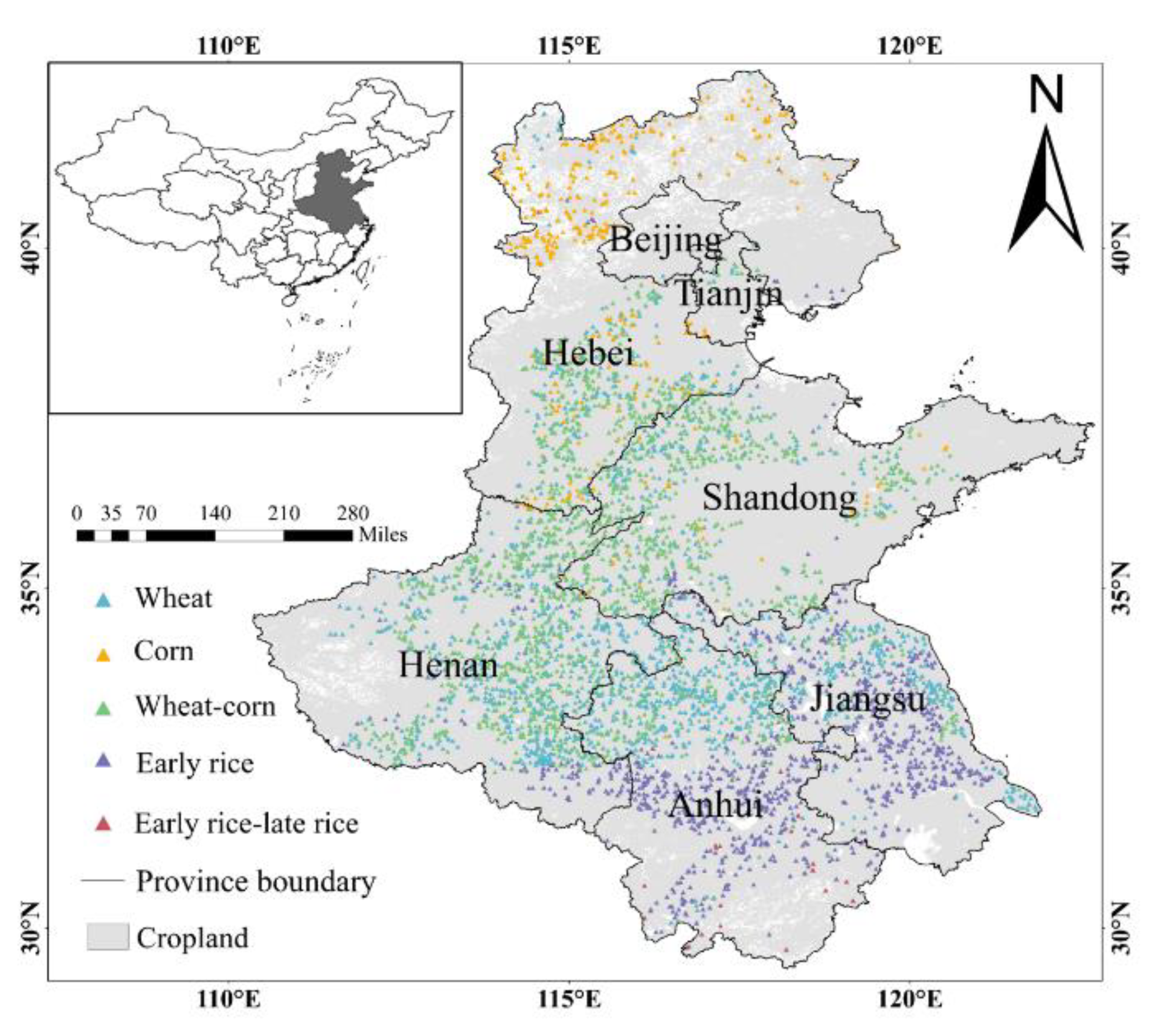
2.1. Study Area

The North China Plain, also known as the Huanghuaihai Region, is an integral part of the Great Eastern Plain in China and is one of the most critical granaries in China (Figure 1). It is composed of seven provinces, including Beijing, Tianjin, Hebei, Shandong, Henan, Anhui, and Jiangsu, with a total area of 7,789,000 km². The North China Plain begins at the Great Wall in the north, reaches Tongbai Mountains in the south, leans on Taihang Mountains in the west, and borders the Bohai Sea and the Yellow Sea in the east. It is a typical alluvial plain formed by the Yellow River, Huai River, Hai River, and their tributaries. This region belongs to temperate continental monsoon type semi-arid and semi-humid climate, with apparent changes in four seasons: a dry spring and little rain, a hot and rainy summer, and colder and drier winter. There are extensive heat and light resources and a high potential for yield increase.

2.2. Data

2.2.1. MODIS Data

The MODIS 16-day composite surface reflectance products with a spatial resolution of 1 km from the Terra satellite (MOD13A2) were utilized for crop classification. All available products from 2015 to 2016 were downloaded from the Google Earth Engine (https://earthengine.google.com/, accessed on 27 January 2021); a total of 46 images were obtained. MOD13A2 has four reflectance bands, including blue, red, near-infrared, and mid-infrared, as well as two vegetation layers, including NDVI and EVI. The MOD13A2 product selects the best available pixel values from all acquisitions over 16 days based on the principles of low clouds, low viewing angles, and highest NDVI/EVI values.

2.2.2. Sample Data

The samples were obtained from the ChinaCropPhen1km distribution map, which contained wheat, corn, and rice for 2015 in the North China Plain. These crop maps have a spatial resolution of 1 km with the Asia North Albers Equal Area Conic projection and R² for this dataset was higher than 0.8 [43]. Each pixel in the crop distribution map is assigned a specific value, with a value of 0 indicating a non-crop growing area and value of 1 indicating a crop growing area. The non-crop growing areas were masked. Due to the bias in the maps, more information needs to be collected. We compared the acreage of each crop with the county-level statistical yearbooks, and the crop areas that did not exist in the statistical county-level regions were removed. After the statistical comparison, among 235,037 cropping pixels, 230,036 crop pixels were left, with an accuracy of 97.845%; thus, we believe the crop distribution map is reliable. Moreover, to avoid other possible errors in Luo’s results [43], test samples were selected from the crop map and visual interpretation from Google Earth and VI curves to determine the crop type of 4813 pixels (see Figure 1).

All samples in the study area were split into three datasets, including training, validation, and test sets. The training set was used to train the classification algorithms. The validation set was used to select the optimal hyperparameters. The final model’s performance was evaluated with the test set. The division of the dataset follows the principle of independent and homogeneous distribution. Since the test set is obtained by visual interpretation using Google Earth, we only divide all the remaining areas into training and validation sets with 80% and 20%, respectively. There are 180,173, 45,050 and 4813 samples in the training, validation and test sets, respectively (

Table 1. Number of data samples and test samples for five crop types.

Abbreviations Used in This Study	Description	Data Set		Test Set
		Number of Pixels	Areal Percentage/%	Number of Pixels	Areal Percentage/%
WT	Wheat	69,117	30.04	1429	29.69
CN	Corn	16,334	7.10	351	7.29
WC	Wheat–Corn	92,791	40.34	1956	40.64
ER	Early rice	50,533	21.97	1051	21.84
EL	Early rice–Late rice	1261	0.55	26	0.54
Total		230,036	100	4813	100

). Since wheat–corn rotation and early rice–late rice rotation in the North China Plain are used in many studies, the three crop classes distribution maps obtained from the ChinaCropPhen1km were combined as five classes, including wheat, corn, wheat–corn, early rice and early rice–late rice.

2.3. Method

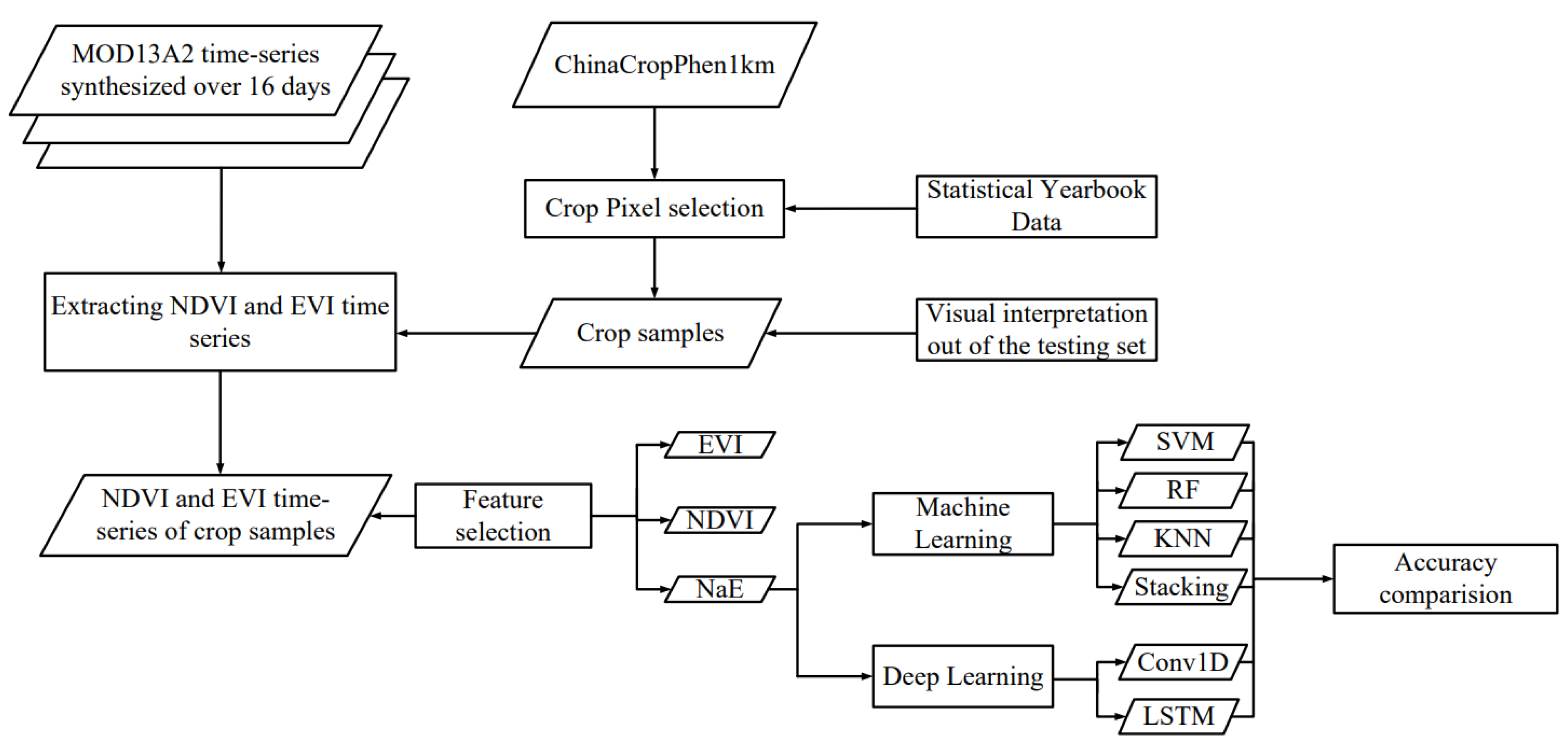
2.3.1. Data Acquisition and Preparation

The overall workflow of this study is shown in Figure 2. Firstly, the crop sample points were selected by the ChinaCropPhen1km dataset and visual interpretation. Second, the MOD13A2 was applied to extract the features of the time series MODIS NDVI, EVI and NaE for the crop sample points. Next, the reconstruction of machine learning and deep learning classifiers including Stacking, SVM, KNN, RF, Conv1D and LSTM was conducted. Then, the time series NDVI, EVI and NaE was fed into the classifier as a feature and the optimal features and model were selected by comparing the performance. Finally, the accuracy of the classification results was evaluated.

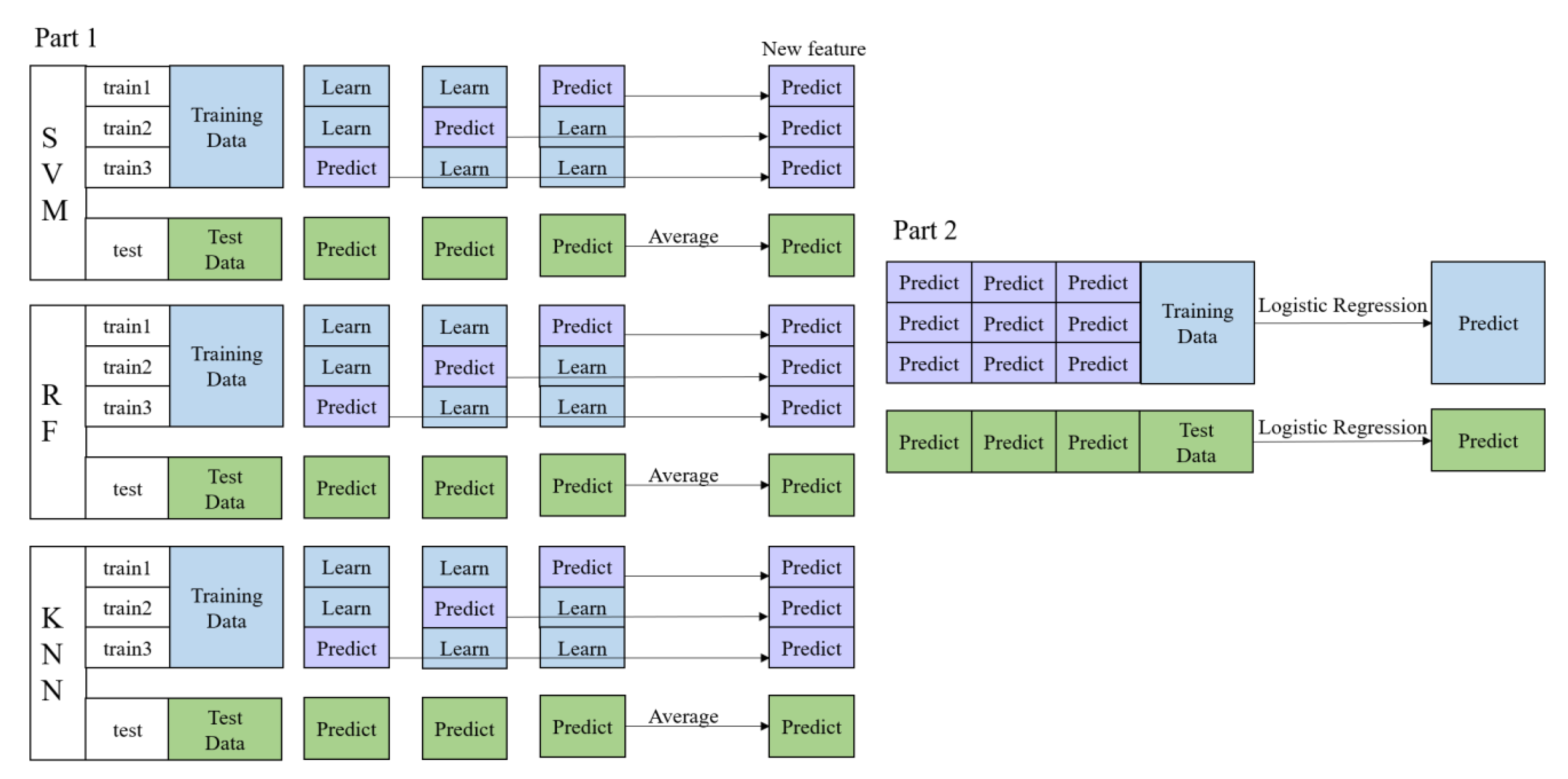
2.3.2. Machine Learning Classifiers

Four machine learning classifiers: SVM, RF, KNN, and Stacking were used in this study. SVM is a generalized linear classifier. When making predictions, SVM maps the data through the kernel function and divides the data through the decision boundary [44]. RF is an integrated algorithm consisting of multiple decision trees (DTs), which generates the final classification results by majority voting [45,46]. The KNN algorithm performs classification by measuring the distance between different samples. When making predictions, the category of a test sample is determined by proximity points [47]. Details of hyper-parameters for SVM, RF, and KNN are presented in

Table 2. Parameter description of the SVM, RF and KNN classifiers.

Classifier	Parameter	Description
SVM	C	C is the penalty coefficient used to control the loss function.
	gamma	gamma denotes the kernel function coefficient.
RF	n_estimators	n_estimators shows the ability and complexity of RF to learn from data.
	min_samples_split	min_samples_split expresses the minimum number of samples needed to split internal nodes.
	min_samples_leaf	min_samples_leaf indicates the minimum sample tree on the leaf nodes.
	max_features	max_features mean the number of features to be considered when finding the optimal splitting point.
KNN	n_neighbors	n_neighbors show the number of neighboring samples.
	leaf_size	leaf_size represents the size of the sphere tree or kd tree.

.

Stacking is the process of feeding the output of the base models as new features into other models. This method realizes the cascading of models, which means that the output of the first layer is used as the input of the second layer, and the last layer outputs the final results [48]. Stacking should prevent the phenomenon of a leak. That means the base model should not duplicate the data used for training when making output predictions. We use the 3-fold cross-validation method to output the results of each part of the sample separately. In this study, the first layer of the base model used SVM, KNN and RF classifiers, and the parameters of the base classifiers are obtained from the above experiments. In the second layer, the LogisticRegression was used for the prediction (Figure 3).

Each classifier requires a set of hyperparameters that need to be configured during the development of the classification model. The optimal values of the hyperparameters were chosen based on the classification accuracy of the validation set. We used a “random search” strategy to optimize the main hyperparameters of the selected classifier: the classifier was trained several times iteratively and each run was randomly sampled from a combination of all hyperparameter values. Random search dramatically improves the efficiency of hyperparameter optimization [25,49].

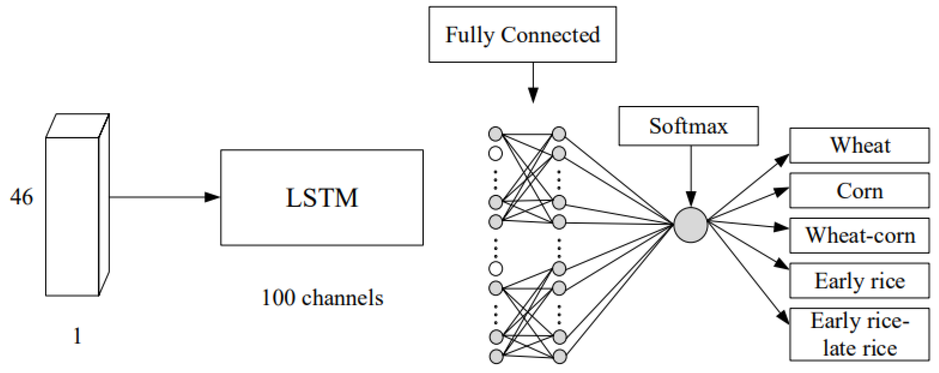
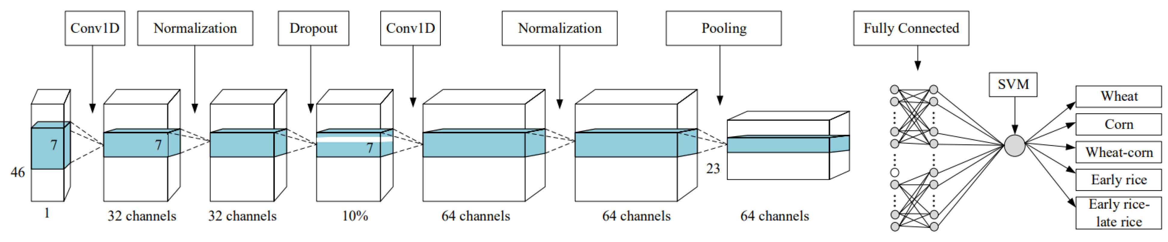
2.3.3. Deep Learning Classifiers

We tested two deep learning classifiers including Conv1D, a form of CNN (Figure 4), and LSTM, a special architecture of RNN (Figure 5). Conv1D and LSTM are two practical approaches in extracting temporal features.

Conv1D uses a one-dimensional filter to extract the features of the time series. Local features are extracted at the bottom of the model. The top layer will fuse the local features to extract the global characteristics of the time series. The optimization of Conv1D-based models is complex. Due to the diversity of architectures, there is no optimal combination of hyperparameters and various layers. In this study, Conv1D is implemented with a combination of convolutional, pooling, normalization, dropout and fully connected layers, where the input is one-dimensional data with a length of 46.

In the convolutional layers, the number of layers is searched from 1 to 4, and the number of neurons per layer varies, with test values of 32, 64, 128 and 256. The first convolutional layer has 32 or 64 channels, and the number of channels increases or remains constant as the number of convolutional layers increases. A normalization layer follows each convolution layer. The pooling layer is fixed to the average pooling. The dropout layer is a common method of avoiding overfitting by randomly discarding neurons for each layer so that the output of that layer does not depend on only a few neurons [50]. The dropout values are set to 0, 10%, 20%, 30% and 40%, 50%, 60%, 70%. The normalization process, average-pooling, and dropout are used to prevent overfitting. The model contains two fully connected layers at the output end. The last layer contains five neurons corresponding to five classes of probabilities, and the activation function uses Softmax or SVM. The penultimate layer collects the information from the previous layers as a flat array. We start building a simple model with a single convolutional layer at first, then by changing one or two hyperparameters, add new layers to generate a more complex network. The LSTM model trained by [51] was used in this study.

Both models were trained using the Adam optimizer. Learning rates of 0.0001, 0.0005, 0.001 and 0.005 were tested. Due to the unbalanced nature of the training set, we used a categorical_crossentropy loss function for the gradient descent process.

2.4. Accuracy Evaluation

Three metrics, including overall accuracy, F1-score and kappa coefficient, were used in this study to evaluate the classifier’s performance [52]. All metrics are analyzed using a weighted average (https://scikit-learn.org/, accessed on 1 March 2021). When the samples are unbalanced, it is not appropriate to assign the same weight to each class, so the weighted-average method is used to assign different weights to each class according to the size of each class. The number of samples in each class is the weight of that class. The overall accuracy is the proportion of the total classes that are correctly predicted, while the F1-score is the harmonic mean of the precision and recall rate, which can highlight the ability to identify spatial distribution models of crops. The kappa coefficient indicates the balance of the confusion matrix and is used for consistency testing.

$$\mathrm{Overall} \mathrm{accuracy}=\frac{\mathrm{TP}+\mathrm{TN}}{\mathrm{TP}+\mathrm{FP}+\mathrm{FN}+\mathrm{TN}}$$

(1)

$$\mathrm{F}1-\mathrm{score}=2 \times \frac{ \mathrm{precision} \times \mathrm{recall}}{\mathrm{precision}+\mathrm{recall}}$$

(2)

$$\mathrm{kappa} \mathrm{coefficient}=\frac{{\mathrm{p}}_0-{ \mathrm{p}}_{\mathrm{e}}}{{1-\mathrm{p}}_{\mathrm{e}}}$$

(3)

where positive and negative indicate the presence or absence of the crop, TP and FP indicate correct and incorrect predictions of positives, and TN and FN indicate correct and incorrect predictions of negatives, respectively. The confusion matrix is shown in

Table 3. Confusion matrix charted by the predicted and actual classification.

		Predicted
		Positive	Negative
Actual	Positive	True positives (TP)	False negatives (FN)
	Negative	False positives (FP)	True negatives (TN)

. The precision rate indicates the proportion of data correctly classified as a percentage of all data, while the recall rate indicates the number of samples in a class correctly classified as a percentage of that class. ${\mathrm{p}}_0$ is the ratio of the diagonal elements of the confusion matrix to the whole matrix elements and ${\mathrm{p}}_{\mathrm{e}}$ is the ratio of the sum of the products of the actual and predicted data volumes corresponding to all categories, respectively, and to the square of the total number of samples.

3. Results

3.1. Feature Selection

NDVI, EVI and NaE (combining NDVI and EVI as an input feature to form a one-dimensional vector of 46 variables) were compared as input features and the optimal features were selected. The three groups of features were used as input to different models to obtain relatively consistent results, so only one model’s classification results were shown. The results of the KNN model are presented, as the KNN model has the shortest training time and the most considerable variation of accuracy. The optimal parameters of the KNN model are shown in

Table 4. Hyperparameter selection of the KNN model for different inputs.

Hyper-Parameter	Candidate Values	Data	Selected Values for Input Sets
N_neighbors Leaf_size	10, 20, 30, 40, 50, 60, 70, 80, 90, 100, 200, 300, 500, 800, 1200 10, 20, 30, 60, 100	EVI NDVI NaE	50 100 100 100 10 30

. The three groups of features show significantly different classification capabilities in this study. The optimized input feature (NaE) has the highest accuracy (

Table 5. Comparison of results of KNN models for crop classification using three groups of features.

	EVI	NDVI	NaE
Overall Accuracy	67.98%	72.31%	76.20%
F1-score	0.6724	0.7159	0.7616
kappa coefficient	0.5317	0.5941	0.6536

) among all features. Additionally, the F1-Score of NaE is more than other features. By contrast, the EVI feature has the lowest accuracy. The influence of clouds, fog and insolation can cause NDVI and EVI to experience certain limitations, while NaE will have another feature for crop classification when there is a problem with one feature, increasing the possibility of correct crop classification. Additionally, NaE will provide more temporal features for the classifier to improve the classification accuracy. Since NaE data showed the best classification results, we used them for crop classification in the later experiments.

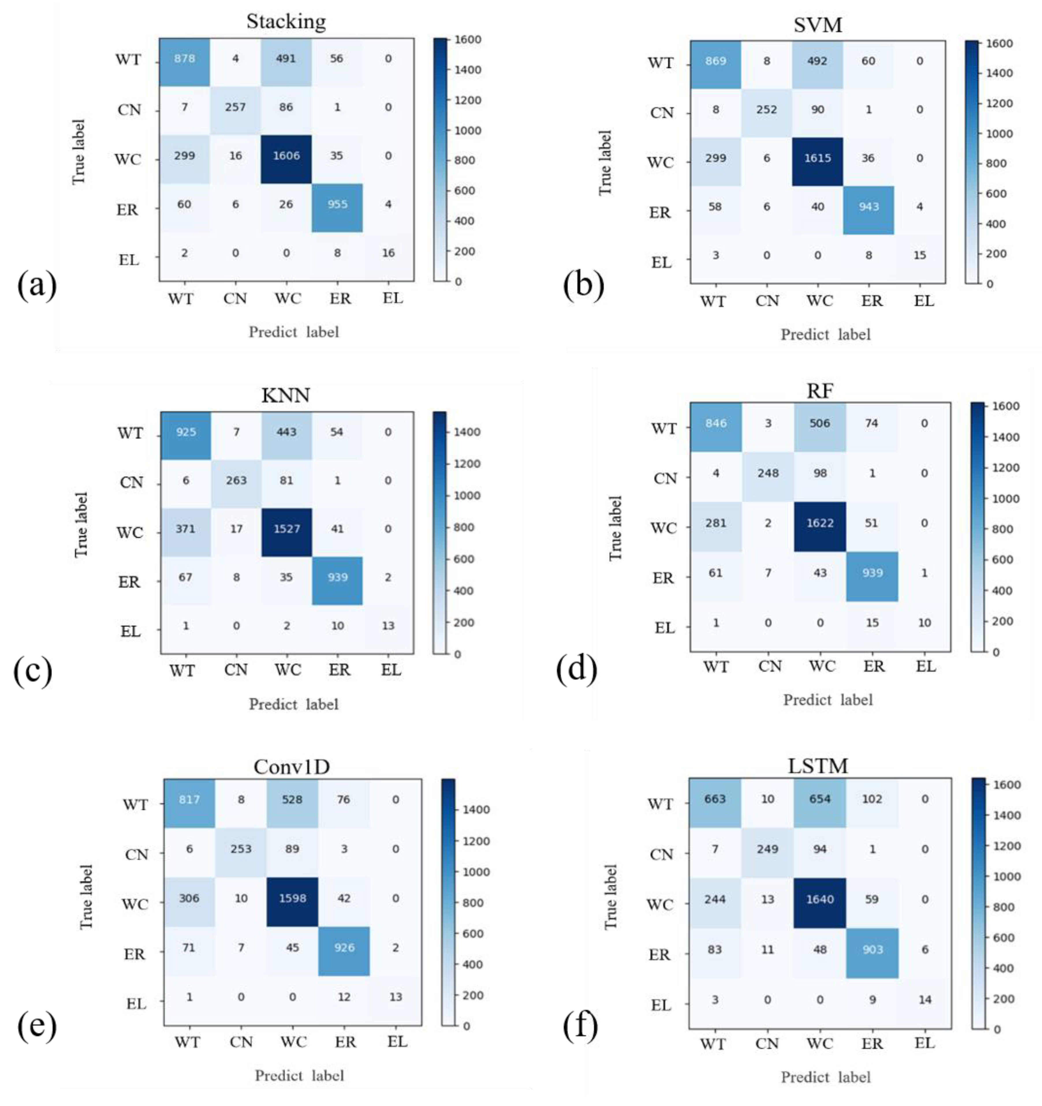
3.2. Machine Learning and Deep Learning Classification Results

The hyperparameters settings of the machine learning classifiers significantly impact the classification results. We used a “random search” strategy for hyperparameters determination, and the optimal hyperparameters of SVM, RF and KNN are attached in Table 4 and

Table 6. Optimal hyperparameter selection for machine learning.

Classifier	Hyper-Parameter	Candidate Values	Selected Values for Input Sets
SVM	C	10, 20, 30, 40, 50, 60, 70, 80, 90, 100, 200, 300, 500, 800, 1200	10
	gamma	0.1, 1, 2, 10, ‘auto’	0.1
RF	N_estimators	100, 200, 300, 400, 500, 600, 700, 800, 900, 1000	800
	Min_samples_split	2, 5, 10, 15, 20, 100	2
	Min_samples_leaf	1, 2, 3, 4, 5, 10	1
	Max_features	‘log2′, ’sqrt’, ’auto’	‘sqrt’

. The hyperparameters of Stacking are the best parameters selected by the three classifiers.

These four classifiers show a significant difference in classification capabilities (Figure 6). Among the four machine learning classifiers, Stacking has the best performance with an accuracy of 77.12%. The Stacking model used the output of other single models as input and combined the original data features to make decisions, so it showed a higher classification accuracy. However, the Stacking model cannot distinguish whether the output of other models was correct, which will reduce accuracy. Hence, the stacking model confusion matrix showed results that are not optimal for almost every class. SVM (76.75%) has slightly worse performance than the Stacking and has the longest training time, which is not suitable for large-scale data training due to the high time complexity. The classification accuracy achieved by the RF (76.15%) and KNN (76.19%) are similar, and the training time of KNN is less than that of RF. Both deep learning models used in this study did not show strong classification capabilities (Figure 6). The Conv1D (74.97%) model has a higher accuracy based on the test set, and the LSTM (73.20%) model has a slightly lower accuracy. It can be seen that Stacking achieved excellent classification performance compared to the other models; in contrast, LSTM had the worst performance (Figure 7). Machine learning models are relatively complex in performing hyperparameter selection, requiring the comparison of many hyperparameters, which is time-consuming, but the accuracy of machine learning is high in this study. Although the LSTM was initially developed for time-series tasks [25], it appears to be not suitable for the current classification experiments.

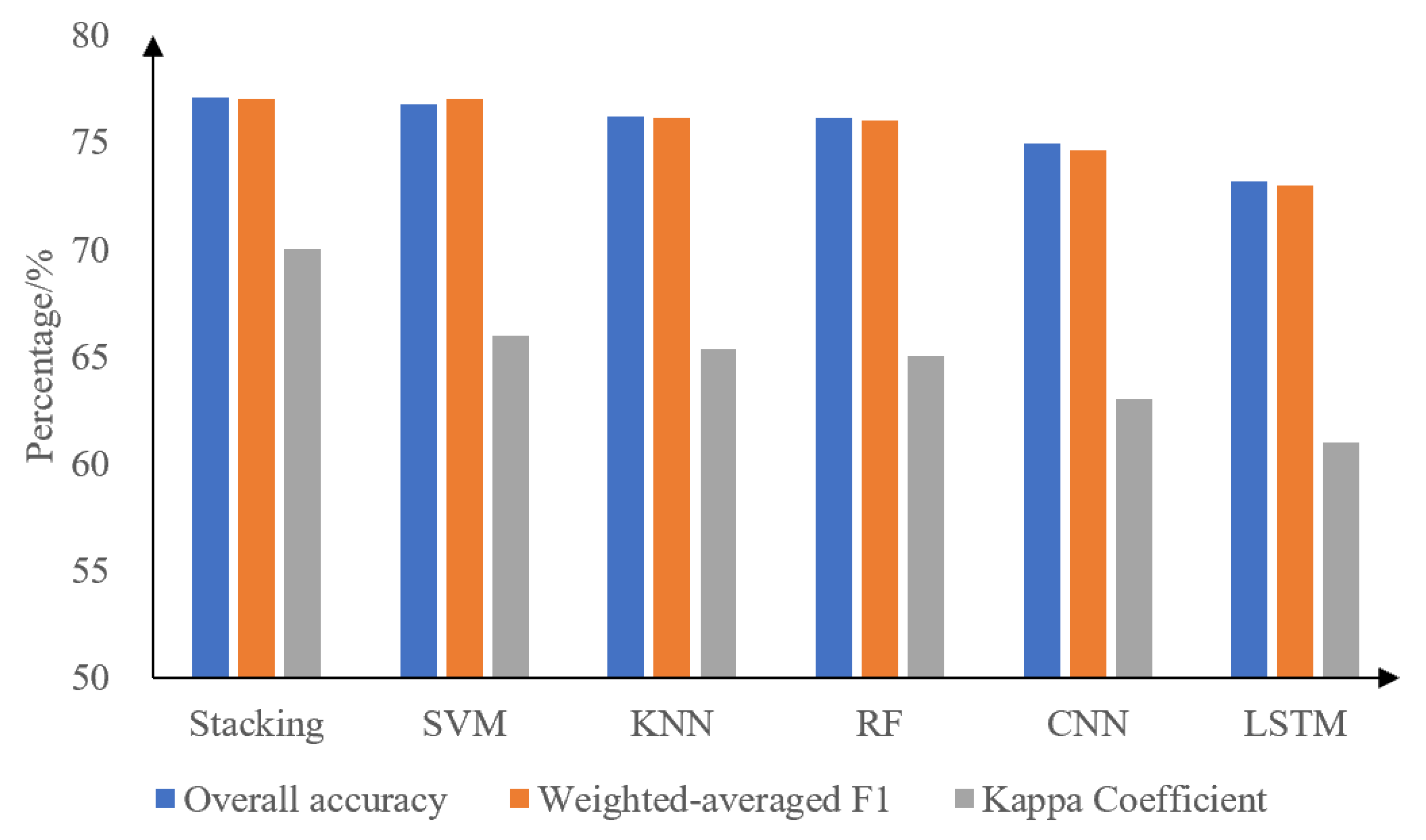
3.3. Comparison of Machine Learning and Deep Learning Results

Among all machine learning and deep learning models, the Stacking method achieved the best classification results (Figure 7). In contrast, two deep learning models performed much worse than those of the machine learning models. The classification accuracy of LSTM was the lowest among all classifiers. A comparison was made between Stacking’s confusion matrix and Conv1D’s confusion matrix, which were the best performing machine learning and deep learning models, respectively.

Table 7. Difference between confusion matrices achieved by the Stacking and the Conv1D classifiers. Values are calculated as Figure 6a minus Figure 6e.

Reference Classes	Predict Classes
	WT	CN	WC	ER	EL
WT	61	−4	−37	−20	0
CN	1	4	−3	−2	0
WC	−7	6	8	−7	0
ER	−11	−1	−19	29	2
EL	1	0	0	−4	3

highlights the differences (Figure 6a minus Figure 6e) to show the relative strength of the two classifiers for each category.

Classification errors, expressed as plots outside the. diagonal of the confusion matrix, can be divided into the following types: (1) classification errors of rotational crops into non-rotational crops and non-rotational crops into rotational crops. (2) Classification errors between non-rotation crops. (3) Misclassification between multiple different crops. Compared to Conv1D, the Stacking method reduced misclassification of non-rotation crops into rotation crops in 68 pixels and misclassification between non-rotation crops in 142 pixels. All the values on the diagonal of Table 7 are positive, and the values on the non-diagonal are primarily negative, indicating that the Stacking outperforms the Conv1D model in differentiating between rotational crops and non-rotational crops. Thus, the Stacking improves the results of crop classification significantly. The plots classified by Stacking, Conv1D and LSTM are shown in Figure 8a–c for visual comparison with the corresponding plots in the reference map in Figure 8d [43].

4. Discussion

4.1. Effectiveness of the Used Models

Six models were used to classify the major crops in the North China Plain, and the weighted average F1-scores and classification overall accuracy of all models were above 0.7, and 70%, respectively. Massey et al. [53] used 250 m of time-series MODIS NDVI data combined with decision tree classification for multi-year crops in the United States and showed that the overall accuracy of was higher than 75%. Xun et al. [54] used the Leaf Area Index (LAI) and sparse representation algorithm to classify crops in the North China Plain from 2016 to 2017 with classification accuracy higher than 76%. Wang et al. [55] used EVI time series curves to classify winter wheat in the North China Plain with an overall accuracy of 76.36%. Compared to traditional classification methods, the method used in this study achieves 77.12% accuracy in classifying large scale multi-type crops, which is feasible and efficient for identifying crop distribution in the study area. Multiple types of crops can be classified without significant time and cost, which effectively reduces computational costs. The results of this study can provide valuable implications for crop classification and yield estimation in the region [54].

The vegetation indices (NaE) were used as inputs to the classifier, which may provide more feature selection opportunities for the classifier. In the classification experiments, Stacking gave the best classification results and LSTM performed the worst. By comparing the classification results of the six models, we found that the Stacking (Figure 6a) effectively distinguished between wheat and wheat–corn rotations and between early and early–late rice rotations. In contrast, deep learning (Figure 6e) has low recognition efficiency of rotation and non-rotation types.

Table 8. Percentage of each category in the crop classification map.

Crop Type	Stacking	Conv1D	LSTM	Reference Map
	Areal Percentage/%
WT	30.01	24.56	21.35	29.69
CN	6.97	6.17	6.29	7.29
WC	40.31	46.54	49.25	40.64
ER	22.18	22.28	22.64	21.84
EL	0.53	0.45	0.47	0.54

shows that the Stacking model achieved crop distribution maps with similar proportions of crops as the reference maps, while the crop distribution maps obtained by LSTM and Conv1D have 5.9% and 8.61% more wheat–corn crops, and 5.13% and 8.34% less wheat crops than the reference maps. Compared with the accuracy of Stacking and Conv1D methods about rotations and non-rotations, the results showed that the accuracy of Stacking (77.75%) is higher than Conv1D (75.32%). Due to the overlap between the growing periods of rotated crops and non-rotated crops, the time-series features of the crop types are somewhat similar. Machine learning is a step-by-step study of temporal features and features are progressively imported into the classifier, which will find the different characteristics of rotation and non-rotation crops and ignore some repeat time-series information about rotation crops and non-rotation crops when performing feature extraction. Deep learning acquires temporal features by activating neurons or channels, which will rely on the channel’s sensitivity response to the input data and may learn repeatable features about rotations and non-rotations.

Although the machine learning models generally gave better results than the deep learning models, the training time and the GPU spent on the machine learning models were longer than the deep learning models. For example, building the RF model is time-consuming because the RF model needs to find the best feature selection and the optimal segmentation point among all the sample plots, while each time needs to construct a decision tree [24]. An early stop technique [56] for Conv1D can be utilized during the model running to automatically end training when the model converges, making the Conv1D model development time efficient. In addition, deep learning models (Conv1D, LSTM) automatically extracted features through backpropagation when training was performed. Therefore, the model is general to various seasonal dynamic modeling research. Using machine classifiers (e.g., RF and SVM), each step-in classification can be considered a relatively independent dimension, and the sequential relationship may not be utilized. Thus, the machine classification algorithm may not be robust to variances caused by weather conditions, agricultural practices, or missing data [25,51].

Furthermore, several factors affect the accuracy of crop classification. Firstly, the growing seasons of crops vary in different regions in the North China Plain, which may cause the same crops in the different latitudes have variance growing seasons. In this experiment, the topography, elevation, climate or different land cover components of the samples can cause the time series to contain bias for the same crop. Therefore, it is necessary to distinguish crops regionally when classifying crops on a large scale in practice, and crops in similar areas with similar NDVI or EVI values will reduce the occurrence of homogeneous situations and will obtain higher accuracy. Secondly, the sample points used to train the classifier were derived from published literature for this work, which may lead to bias in the crop classes of the training sample points; therefore, location accuracy needs to be assessed with additional reference datasets. In addition, the raw data for the crop spatial resolution points are 1 km in pixels, and the sample is too large to avoid the mixed pixels. In crop classification tasks on a large regional scale, low spatial resolution data have the advantage of wide coverage and better quality and would be more conducive to experiments, which would be flawed in practice. In practice, when carrying out crop classification on large scale areas, local areas can be divided and classification experiments can be carried out using higher resolution data. The imagery with a higher spatial resolution can be adopted in future studies for accuracy improvement and generalizability of the model.

4.2. Potential Refinements

There is a wide range of strategies in machine learning and deep learning to improve classification accuracy. A manual selection of hyperparameters is required for Stacking models; however, there are a variety of approaches for automatically conducting hyperparameter optimization in machine learning, including genetic algorithms [3], particle swarm optimization, and simulated annealing, which can all be explored in future research process optimization. In remote sensing crop classification studies, CNNs models are commonly used in spatial and spectral domains. CNNs are the most widely employed models in deep learning for remote sensing image classification, and future research will be able to merge 2D photos and time series to produce 3D data for crop classification. In addition, the prediction process of the model is not examined, and future research may devote more attention to the inference mechanism of the model.

5. Conclusions

The accurate spatial distribution information of crops is essential for food security and agricultural management. In this study, the effectiveness of the machine learning and deep learning combined time series data for multiple crop type classification over a large-scale region was investigated. Experimentation with three groups of features based on the time series data from satellite images and adopting four machine learning, two deep learning classifiers to identify five crop types’ classification over the North China Plain. In terms of feature selection, the best crop classification results were obtained by the NaE feature. Among six selected ML and DL models, the Stacking classifier performs the best with 77.12% accuracy. These results showed the great potential of combining time-series NaE data with the Stacking algorithm for large-scale region multiple crop-type classification research. Future work could adapt the method in this study to higher spatial resolution RS image and other crop classification studies.

References

1. Xun, L.; Zhang, J.; Cao, D.; Wang, J.; Zhang, S.; Yao, F. Mapping Cotton Cultivated Area Combining Remote Sensing with a Fused Representation-Based Classification Algorithm. Comput. Electron. Agric. 2021, 181, 105940. [Google Scholar] [CrossRef]
2. Xun, L.; Zhang, J.; Cao, D.; Yang, S.; Yao, F. A Novel Cotton Mapping Index Combining Sentinel-1 SAR and Sentinel-2 Multispectral Imagery. ISPRS J. Photogramm. Remote Sens. 2021, 181, 148–166. [Google Scholar] [CrossRef]
3. Wu, Z.; Zhang, J.; Deng, F.; Zhang, S.; Zhang, D.; Xun, L.; Ji, M.; Feng, Q. Superpixel-Based Regional-Scale Grassland Community Classification Using Genetic Programming with Sentinel-1 SAR and Sentinel-2 Multispectral Images. Remote Sens. 2021, 13, 67. [Google Scholar] [CrossRef]
4. Xun, L.; Zhang, J.; Cao, D.; Zhang, S.; Yao, F. Crop Area Identification Based on Time Series EVI2 and Sparse Representation Approach: A Case Study in Shandong Province, China. IEEE Access 2019, 7, 157513–157523. [Google Scholar] [CrossRef]
5. Felegari, S.; Sharifi, A.; Moravej, K.; Amin, M.; Golchin, A.; Muzirafuti, A.; Tariq, A.; Zhao, N. Integration of Sentinel 1 and Sentinel 2 Satellite Images for Crop Mapping. Appl. Sci. 2021, 11, 104. [Google Scholar] [CrossRef]
6. Valero, S.; Arnaud, L.; Planells, M.; Ceschia, E. Synergy of Sentinel-1 and Sentinel-2 Imagery for Early Seasonal Agricultural Crop Mapping. Remote Sens. 2021, 13, 4891. [Google Scholar] [CrossRef]
7. Eerens, H.; Haesen, D.; Rembold, F.; Urbano, F.; Tote, C.; Bydekerke, L. Image Time Series Processing for Agriculture Monitoring. Environ. Model. Softw. 2014, 53, 154–162. [Google Scholar] [CrossRef]
8. Zhang, G.; Xiao, X.; Dong, J.; Kou, W.; Jin, C.; Qin, Y.; Zhou, Y.; Wang, J.; Menarguez, M.A.; Biradar, C. Mapping Paddy Rice Planting Areas through Time Series Analysis of MODIS Land Surface Temperature and Vegetation Index Data. ISPRS J. Photogramm. Remote Sens. 2015, 106, 157–171. [Google Scholar] [CrossRef] [Green Version]
9. Wang, X.; Zhang, S.; Feng, L.; Zhang, J.; Deng, F. Mapping Maize Cultivated Area Combining MODIS EVI Time Series and the Spatial Variations of Phenology over Huanghuaihai Plain. Appl. Sci. 2020, 10, 2667. [Google Scholar] [CrossRef]
10. Zhang, J.; Feng, L.; Yao, F. Improved Maize Cultivated Area Estimation over a Large Scale Combining MODIS-EVI Time Series Data and Crop Phenological Information. ISPRS J. Photogramm. Remote Sens. 2014, 94, 102–113. [Google Scholar] [CrossRef]
11. Wu, Z.; Zhang, J.; Deng, F.; Zhang, S.; Zhang, D.; Xun, L.; Javed, T.; Liu, G.; Liu, D.; Ji, M. Fusion of Gf and Modis Data for Regional-Scale Grassland Community Classification with Evi2 Time-Series and Phenological Features. Remote Sens. 2021, 13, 835. [Google Scholar] [CrossRef]
12. Qiu, B.; Feng, M.; Tang, Z. A Simple Smoother Based on Continuous Wavelet Transform: Comparative Evaluation Based on the Fidelity, Smoothness and Efficiency in Phenological Estimation. Int. J. Appl. Earth Obs. Geoinf. 2016, 47, 91–101. [Google Scholar] [CrossRef]
13. Potgieter, A.B.; Apan, A.; Hammer, G.; Dunn, P. Early-Season Crop Area Estimates for Winter Crops in NE Australia Using MODIS Satellite Imagery. ISPRS J. Photogramm. Remote Sens. 2010, 65, 380–387. [Google Scholar] [CrossRef]
14. Sakamoto, T.; Yokozawa, M.; Toritani, H.; Shibayama, M.; Ishitsuka, N.; Ohno, H. A Crop Phenology Detection Method Using Time-Series MODIS Data. Remote Sens. Environ. 2005, 96, 366–374. [Google Scholar] [CrossRef]
15. Funk, C.; Budde, M.E. Phenologically-Tuned MODIS NDVI-Based Production Anomaly Estimates for Zimbabwe. Remote Sens. Environ. 2009, 113, 115–125. [Google Scholar] [CrossRef]
16. Jönsson, P.; Eklundh, L. Seasonality Extraction by Function Fitting to Time-Series of Satellite Sensor Data. IEEE Trans. Geosci. Remote Sens. 2002, 40, 1824–1832. [Google Scholar] [CrossRef]
17. Jönsson, P.; Eklundh, L. TIMESAT—A Program for Analyzing Time-Series of Satellite Sensor Data. Comput. Geosci. 2004, 30, 833–845. [Google Scholar] [CrossRef] [Green Version]
18. Sakamoto, T.; Van Nguyen, N.; Ohno, H.; Ishitsuka, N.; Yokozawa, M. Spatio-Temporal Distribution of Rice Phenology and Cropping Systems in the Mekong Delta with Special Reference to the Seasonal Water Flow of the Mekong and Bassac Rivers. Remote Sens. Environ. 2006, 100, 1–16. [Google Scholar] [CrossRef]
19. Galford, G.L.; Mustard, J.F.; Melillo, J.; Gendrin, A.; Cerri, C.C.; Cerri, C.E.P. Wavelet Analysis of MODIS Time Series to Detect Expansion and Intensification of Row-Crop Agriculture in Brazil. Remote Sens. Environ. 2008, 112, 576–587. [Google Scholar] [CrossRef]
20. Shao, Y.; Lunetta, R.S.; Wheeler, B.; Iiames, J.S.; Campbell, J.B. An Evaluation of Time-Series Smoothing Algorithms for Land-Cover Classifications Using MODIS-NDVI Multi-Temporal Data. Remote Sens. Environ. 2016, 174, 258–265. [Google Scholar] [CrossRef]
21. Chen, J.; Jönsson, P.; Tamura, M.; Gu, Z.; Matsushita, B.; Eklundh, L. A Simple Method for Reconstructing a High-Quality NDVI Time-Series Data Set Based on the Savitzky-Golay Filter. Remote Sens. Environ. 2004, 91, 332–344. [Google Scholar] [CrossRef]
22. Olsson, L. Fourier Series for Analysis of Temporal Sequences of Satellite Sensor Imagery. Int. J. Remote Sens. 1994, 15, 3735–3741. [Google Scholar] [CrossRef]
23. Verhoef, W.; Menenti, M.; Azzali, S. Cover a Colour Composite of NOAA-AVHRR-NDVI Based on Time Series Analysis (1981–1992). Int. J. Remote Sens. 1996, 17, 231–235. [Google Scholar] [CrossRef]
24. He, T.; Xie, C.; Liu, Q.; Guan, S.; Liu, G. Evaluation and Comparison of Random Forest and A-LSTM Networks for Large-Scale Winter Wheat Identification. Remote Sens. 2019, 11, 1665. [Google Scholar] [CrossRef] [Green Version]
25. Zhong, L.; Hu, L.; Zhou, H. Deep Learning Based Multi-Temporal Crop Classification. Remote Sens. Environ. 2019, 221, 430–443. [Google Scholar] [CrossRef]
26. Guidici, D.; Clark, M.L. One-Dimensional Convolutional Neural Network Land-Cover Classification of Multi-Seasonal Hyperspectral Imagery in the San Francisco Bay Area, California. Remote Sens. 2017, 9, 629. [Google Scholar] [CrossRef] [Green Version]
27. Kumar, S.; Shukla, S.; Sharma, K.K.; Singh, K.K.; Akbari, A.S. Classification of Land Cover and Land Use Using Deep Learning. In Machine Vision and Augmented Intelligence—Theory and Applications; Springer: Berlin/Heidelberg, Germany, 2021; pp. 321–327. [Google Scholar] [CrossRef]
28. Bermúdez, J.D.; Achanccaray, P.; Sanches, I.D.; Cue, L.; Happ, P.; Feitosa, R.Q. Evaluation of Recurrent Neural Networks for Crop Recognition from Multitemporal Remote Sensing Images. An. Do Congr. Bras. De Cartogr. E XXVI Expo. 2017, 2017, 800–804. [Google Scholar]
29. Chen, S.W.; Tao, C.S. Multi-Temporal PolSAR Crops Classification Using Polarimetric-Feature-Driven Deep Convolutional Neural Network. In Proceedings of the RSIP 2017—International Workshop on Remote Sensing with Intelligent Processing, Shanghai, China, 18–21 May 2017. [Google Scholar] [CrossRef]
30. Ji, S.; Zhang, C.; Xu, A.; Shi, Y.; Duan, Y. 3D Convolutional Neural Networks for Crop Classification with Multi-Temporal Remote Sensing Images. Remote Sens. 2018, 10, 75. [Google Scholar] [CrossRef] [Green Version]
31. Mou, L.; Bruzzone, L.; Zhu, X.X. Learning Spectral-Spatialoral Features via a Recurrent Convolutional Neural Network for Change Detection in Multispectral Imagery. IEEE Trans. Geosci. Remote Sens. 2019, 57, 924–935. [Google Scholar] [CrossRef] [Green Version]
32. Breiman, L. Random forests, machine learning 45. J. Clin. Microbiol. 2001, 2, 199–228. [Google Scholar]
33. Mitchell, T.M. Machine Learning; McGraw-Hill: New York, NY, USA, 2003. [Google Scholar]
34. Zhong, L.; Hawkins, T.; Biging, G.; Gong, P. A Phenology-Based Approach to Map Crop Types in the San Joaquin Valley, California. Int. J. Remote Sens. 2011, 32, 7777–7804. [Google Scholar] [CrossRef]
35. Lu, H.; He, J.; Liu, L. Discussion on multispectral remote sensing image classification integrating object-oriented image analysis and KNN algorithm. Sci. Technol. Innov. Appl. 2019, 11, 27–30. [Google Scholar]
36. Chan, J.C.W.; Paelinckx, D. Evaluation of Random Forest and Adaboost Tree-Based Ensemble Classification and Spectral Band Selection for Ecotope Mapping Using Airborne Hyperspectral Imagery. Remote Sens. Environ. 2008, 112, 2999–3011. [Google Scholar] [CrossRef]
37. Juan, P.; Yang, C.; Song, Y.; Zhai, Z.; Xu, H. Classification of rice phenotypic omics entities based on stacking integrated learning. Trans. Chin. Soc. Agric. Mach. 2019, 50, 9. [Google Scholar]
38. Löw, F.; Michel, U.; Dech, S.; Conrad, C. Impact of Feature Selection on the Accuracy and Spatial Uncertainty of Per-Field Crop Classification Using Support Vector Machines. ISPRS J. Photogramm. Remote Sens. 2013, 85, 102–119. [Google Scholar] [CrossRef]
39. LeCun, Y.; Bengio, Y. Convolutional networks for images, speech, and time series. In The Handbook of Brain Theory and Neural Networks; MIT Press: Cambridge, MA, USA, 1995; Volume 3361. [Google Scholar]
40. Karim, F.; Majumdar, S.; Darabi, H.; Harford, S. Multivariate LSTM-FCNs for Time Series Classification. Neural Netw. 2019, 116, 237–245. [Google Scholar] [CrossRef] [Green Version]
41. Rodriguez-Galiano, V.F.; Ghimire, B.; Rogan, J.; Chica-Olmo, M.; Rigol-Sanchez, J.P. An Assessment of the Effectiveness of a Random Forest Classifier for Land-Cover Classification. ISPRS J. Photogramm. Remote Sens. 2012, 67, 93–104. [Google Scholar] [CrossRef]
42. Tuanmu, M.N.; Viña, A.; Bearer, S.; Xu, W.; Ouyang, Z.; Zhang, H.; Liu, J. Mapping Understory Vegetation Using Phenological Characteristics Derived from Remotely Sensed Data. Remote Sens. Environ. 2010, 114, 1833–1844. [Google Scholar] [CrossRef]
43. Luo, Y.; Zhang, Z.; Li, Z.; Chen, Y.; Zhang, L.; Cao, J.; Tao, F. Identifying the Spatiotemporal Changes of Annual Harvesting Areas for Three Staple Crops in China by Integrating Multi-Data Sources. Environ. Res. Lett. 2020, 15, 074003. [Google Scholar] [CrossRef]
44. Smola, A.J.; Schölkopf, B. A Tutorial on Support Vector Regression. Stat. Comput. 2004, 14, 199–222. [Google Scholar] [CrossRef] [Green Version]
45. Krzywinski, M.; Altman, N. Classification and Regression Trees. Nat. Methods 2017, 14, 757–758. [Google Scholar] [CrossRef]
46. Jin, S.; Yang, L.; Zhu, Z.; Homer, C. A Land Cover Change Detection and Classification Protocol for Updating Alaska NLCD 2001 to 2011. Remote Sens. Environ. 2017, 195, 44–55. [Google Scholar] [CrossRef]
47. Tomek, I. A Generalization of the K-NNRule. IEEE Trans. Syst. Man Cybern. 1976, SMC-6, 121–126. [Google Scholar] [CrossRef]
48. Menahem, E.; Rokach, L.; Elovici, Y. Troika—An Improved Stacking Schema for Classification Tasks. Inf. Sci. 2009, 179, 4097–4122. [Google Scholar] [CrossRef] [Green Version]
49. Bergstra, J.; Bengio, Y. Random Search for Hyper-Parameter Optimization. J. Mach. Learn. Res. 2012, 13, 281–305. [Google Scholar]
50. Srivastava, N.; Hinton, G.; Krizhevsky, A.; Sutskever, I.; Salakhutdinov, R. Dropout: A Simple Way to Prevent Neural Networks from Overfitting. Phys. Lett. B 2014, 299, 345–350. [Google Scholar] [CrossRef]
51. Gadiraju, K.K.; Ramachandra, B.; Chen, Z.; Vatsavai, R.R. Multimodal Deep Learning Based Crop Classification Using Multispectral and Multitemporal Satellite Imagery. In Proceedings of the ACM SIGKDD International Conference on Knowledge Discovery and Data Mining, Virtual Event, 6–10 July 2020; pp. 3234–3242. [Google Scholar] [CrossRef]
52. Powers, D.M.W. Evaluation: From Precision, Recall and F-Measure to ROC, Informedness, Markedness and Correlation. arXiv 2020, arXiv:2010.16061. Available online: https://arxiv.org/abs/2010.16061 (accessed on 1 March 2021).
53. Massey, R.; Sankey, T.T.; Congalton, R.G.; Yadav, K.; Thenkabail, P.S.; Ozdogan, M.; Meador, A.J.S. MODISphenology-derived, multi-year distribution of conterminous US crop types. Remote Sens. Environ. 2017, 198, 490–503. [Google Scholar] [CrossRef]
54. Xun, L.; Wang, P.; Li, L.; Wang, L.; Kong, Q. Identifying crop planting areas using Fourier-transformed feature of time series MODIS leaf area index and sparse-representation-based classification in the North China Plain. Int. J. Remote Sens. 2019, 40, 2034–2052. [Google Scholar] [CrossRef]
55. Wang, X.; Li, X.B.; Tan, M.H.; Xin, L.J. Remote sensing monitoring of winter wheat sowing area changes in the North China Plain from 2001 to 2011. J. Agric. Eng. 2015, 31, 190–199. [Google Scholar]
56. Yao, Y.; Rosasco, L.; Caponnetto, A. On Early Stopping in Gradient Descent Learning. Constr. Approx. 2007, 26, 289–315. [Google Scholar] [CrossRef]
Figure 1. Location of the study area, cropland cover and sampled plots in North China Plain.
Remotesensing 14 02341 g001
Figure 2. General workflow of this study.
Remotesensing 14 02341 g002
Figure 3. Architecture of the Stacking model. Part 1 obtains the prediction results using SVM, KNN, and RF as base classifiers. Part 2 is to obtain the prediction results by Logistic Regression using both the prediction results of the base classifier and the original data as the data input.
Remotesensing 14 02341 g003
Figure 4. Architecture of the Conv1D-based model used for crop classification in this study.
Remotesensing 14 02341 g004
Figure 5. Architecture of the LSTM model used for crop classification in this study.
Remotesensing 14 02341 g005
Figure 6. Confusion matrix obtained by the Stacking (a), SVM (b), KNN (c), RF (d), Conv1D (e) and LSTM (f) model using NaE as input feature.
Remotesensing 14 02341 g006
Figure 7. Overall accuracy, weighted-average F1 score values and kappa coefficient achieved by different classifiers using NaE as input.
Remotesensing 14 02341 g007
Figure 8. Crop Classification map generated by the Stacking (a), Conv1D (b), LSTM (c) models and reference data (d).
Remotesensing 14 02341 g008