Abstract
The coarse resolution of land surface temperatures (LSTs) retrieved from thermal-infrared (TIR) satellite images restricts their usage. One way to improve the resolution of such LSTs is downscaling using high-resolution remote sensing images. Herein, Gaofen-6 (GF-6) and Landsat-8 images were used to obtain original and retrieved LSTs (Landsat-8- and GF-6-retrieved-LSTs) to perform LST downscaling in the Ebinur Lake Watershed. Downscaling model was constructed, and the regression kernel was explored. The results of downscaling LST using the GF-6 normalized difference vegetation index with red-edge band 2, ratio built-up index, normalized difference sand index, and normalized difference water index as multi-remote sensing indices with multiple remote sensing indices with random forest regression method provided optimal downscaling results, with R2 of 0.836, 0.918, and 0.941, root mean square difference of 1.04 K, 2.06 K, and 1.80 K, and the number of pixels with LST errors between −1 K and +1 K of 87.2%, 76.4%, and 81.9%, respectively. The expression of spatial distribution of 16 m-LST downscaling results corresponded with that of Landsat-8- and GF-6-retrieved-LST, and provided additional details spatial description of LST variations, which was absent in the Landsat-8- and GF-6-retrieved LSTs. The results of downscaling LST could satisfy the application requirements of LST spatial resolution.
1. Introduction
Land surface temperature (LST) is a critical parameter in the surface energy balance. It is also an important indicator of land degradation, salinization, desertification, and erosion, and is widely used in studies focusing on evaporation estimates, water cycle, drought monitoring, the “urban heat island” effect [1,2], and the cold island effect in oasis [3]. In early studies, surface temperature was mostly obtained by the ground measurement method, which is associated with an insufficient density of stations and limited space-time range for monitoring spatiotemporal changes of surface thermal environment [4]. With the development of remote sensing technology, satellite images with thermal infrared sensor (TIRS) have become an important approach for obtaining LST because of its wide coverage, relatively low cost, and periodic acquisition [5,6].
Human activities and urban expansion substantially changes the natural surface, causing a series of environmental impacts. The spatial and temporal distribution of thermal environment varies widely with the heterogeneity of underlying surface components and complexity of atmospheric conditions [7,8,9]. However, the LST retrieved from TIRS images typically show a coarse resolution. The Landsat-8 TIRS images provided by the United States Geological Survey website (USGS) (http://earthexplorer.usgs.gov, accessed on 12 March 2022) has been resampled to a resolution of 30 m by the cubic convolution method, although the information expressed remains similar to the physical resolution of the sensor at 100 m, with far lower resolution than the actual spatial model with a resolution of 30 m [10]. This leads to large errors on the spatial scale in the monitoring of high spatial and temporal heterogeneity of the surface environment, which limits the full application of LST. Therefore, LST with high spatial resolution is needed for further study.
To improve this, one of the major areas of interest of TIR-based remote sensing studies is to use high-resolution remote sensing images to downscale low- and mid-resolution IR remote sensing images. The construction of China’s high-resolution earth observation system for major science and technology projects began in 2013. The Gaofen-1 satellite launched in 2013 exhibits high spatial resolution, high time resolution, and large-width imaging, whereas the Gaofen-6 satellite launched in 2018 shows high-spatial resolution, large-width resolution, and high-frequency imaging and is equipped with 2 m-resolution panchromatic/8 m-resolution multi-spectral high-resolution cameras (PMS) and a 16 m-resolution wide field view (WFV) multispectral camera. In addition, purple band, yellow band, and two red-edge bands (0.710 and 0.750 μm) are added based on the Gaofen-1 satellite, making it suitable for large-scale ground object observation and environmental monitoring. These images provide a basis for researchers to use domestic high-resolution images to study LST scaling. How to use domestic high-resolution satellite images with high spatial resolution to achieve spatial downscaling of low-resolution thermal infrared remote sensing images and obtain high-resolution land surface temperature information remains to be determined in thermal infrared remote sensing research. Gaofen-1 (GF-1), Gaofen-2 (GF-2), and Ziyuan-3 (ZY-3) have been used in LST downscaling studies [11,12]. Many scholars have utilized GF-6 in crop and forest classification and extraction of built-up area [13,14,15,16]. Application of the GF-6 in LST downscaling, particularly the effect of the new red-edge bands, requires further analysis.
At present, pixel-level LST downscaling is typically performed using mathematical statistics, pixel-block intensity modulation, or spectral mixing models [17]. Statistical models, such as DisTrad [18], TsHARP [19], and multiple remote sensing indices with random forest regression (MIRF) [20], are generally straightforward to use and have acceptable levels of precision. The DisTrad method achieves LST downscaling based on the statistical law of scale invariance between the normalized difference vegetation index (NDVI) and LST at different scales; however, there are deficiencies in spatial variation of expression. The TsHARP method improves upon the DisTrad method by replacing NDVI with vegetation coverage and obtains better downscaling results. Considering that LST is affected by multiple factors, the MIRF method uses multiple remote sensing indices as regression kernel for scaling down. The influence of different surface characteristic factors on LST distribution changes under various underlying surfaces. Rather than using normalized difference dust index (NDDI), Pan [21] proposed a downscaling method based on normalized difference sand index in MIRF (NDSI-RF) for arid sandy deserts, which enabled highly precise downscaling in arid desert-oasis ecotones, and the applicability of NDSI factor and MIRF methods in different seasons, distinct regions, and various sensors has been comprehensively studied [20,21,22]. Chen [23] conducted a comparison between DisTrad, TsHARP, and MIRF using multiple levels of resolution, and MIRF produced highly precise downscaled results.
The Ebinur Lake watershed is a classic example of an ecosystem of wetlands in the arid zone, along the New Eurasian Land Bridge, one of China’s Belt and Road Initiative (BRI) economic corridors. It lies at the heart of the Silk Road Economic Belt and is an important part of the Tianshan Northern Slope Economic Zone (TNSEZ). The watershed is endorheic, and it serves as a salt water catchment area for the western part of the TNSEZ [24]. This region is highly sensitive to climate change, and the fragility of the region has been exacerbated by the recent excessive water consumption, which has disrupted the balance between water allocated for ecological, industrial, and domestic usage. These issues have resulted in Lake Ebinur drying out, degradation of vegetation on large scales, desertification, and soil salination. The Ebinur Lake watershed, Beijing-Tianjin-Tanggu region, and Sanjiangyuan region have been included in the sixteen national-priority ecological management zones of China within China’s National Plan for Long- and Medium- Term Forestry Development, and since the state-level Lake Ebinur Wetlands nature reserve was established in 2007, conservation plans have enabled the recovery of the area of Lake Ebinur to a certain extent. However, the rate of recovery of the lake is still far slower than its rate of degradation.
The dynamic succession process of wetland ecosystem caused by lake surface area fluctuation has become the barometer of ecological environment improvement and deterioration, and have attracted widespread interest from academia, governmental organizations, the media, and the public. Numerous studies have been conducted on drainage system changes, soil salination, dust storms, desertification, landscape patterns, and the cool island effect, in the context of this region’s deteriorating ecological environment [25,26,27,28,29,30,31]. However, studies on drought assessment, irrigation monitoring, and water and heat balance require practical application of LST at the field scale, such as soil moisture monitoring at the field scale [32]. This requires the spatial downscaling of LST to meet the resolution requirements for water resource management of the small-scale, highly heterogeneous underlying surfaces, for which study area are lacking. The acquisition of high resolution LST is helpful for analysis complex interactions between human (socio-economic) and natural (ecological) systems, which is a prerequisite for environmental protection and restoration in the study area.
In order to understand the relationship between surface variability caused by human activities and LST, this study took the Ebinur Lake watershed as the study area; Landsat-8 and GF-6 WFV images were used as data sources to perform LST downscaling using the DisTrad, TsHARP, and MIRF methods, respectively. Remote sensing indices, such as the GF-6 NDVI, normalized difference vegetation index with red-edge band 1 (NDVIRE1), normalized difference vegetation index with red-edge band 2 (NDVIRE2), NDSI, ratio built-up index (RBI), and normalized difference water index (NDWI), were selected as regression kernels according to the characteristics of band of GF-6 WFV images and underlying surface features of the study area. This study provides a preliminary data on the viability of using GF-6 images for LST downscaling in the study area, and the effects of the two newly added red-edge bands on the downscaling results with three methods were evaluated, to obtain satisfactory downscaling results for subsequent applications.
2. Materials and Methods
2.1. Overview of the Study Area
The study area is the Ebinur Lake watershed, which is a classic example of an arid oasis. The area lies within the north temperate zone and has a desert-continental climate. It is located in the Bortala Mongol Autonomous Prefecture in the Xinjiang Uyghur Autonomous Region (81°46′–83°51′E, 44°02′–45°10′N). The Gurbantünggüt Desert, Borohoro Mountains (western branch of the Tian Shan Mountain system), Dzungarian Alatau (northern-most branch of the Tian Shan Mountain system), and Mount Mayili (western mountains of Dzungaria) lie to the east, south, west, and north of the study area, respectively. Alashankou valley (with a width of approximately 10 km) is located between the Dzungarian Alatau and Mount Mayili, as shown in Figure 1.
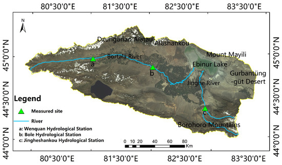
Figure 1.
Study area and locations of ground measurement stations.
The study area is situated in the wetland ecotone of Ebinur Lake. This region has an extremely fragile ecological environment that has been strongly affected by human activities and environmental factors. Owing to its unique geographical location, this study area is extremely important for conducting research on climate regulation, reducing the occurrence of salt-dust storms, and conserving the endemic biodiversity [33].
Agricultural and industrial sectors have developed rapidly together with the population in this region in recent years, and the amount of water consumption for agricultural, municipal, and industrial needs in regions upstream of Ebinur Lake has also increased. Due to this stress, Kuitun River, which is one of the rivers feeding Lake Ebinur, has been completely cut off, leaving only the Bortala River and Jinghe River to feed Ebinur Lake. Combined with a large amount of evaporation and dust weather, the lake area is shrinking rapidly, lakeshore region has become severely desertified, and the salt desert formed on the dried lakebed has become a major source of severe aeolian sandstorms. Therefore, the regional ecological issues caused by changes in the lake-area of Ebinur Lake have become a direct threat to the sustainable development of the TNSEZ and the safety of the New Eurasian Land Bridge [34]. Understanding human and social dynamics, quantifying and mapping the spatial-temporal distribution of environmental vulnerability caused by natural and man-made impacts are needed for environmental protection and restoration [35,36,37,38].
2.2. Data Sources and Preprocessing
2.2.1. Data Sources
The time of passing territory of Landsat-8 and GF-6 in the study area were similar at 13:14:40 and 13:43:20 (Beijing Time), respectively, providing a reliable data source for this study. Landsat-8 images can be contaminated with cloud, particularly in the winter in the study area. Considering the season and quality of image acquisition, images with thick aerosol or heavy cloud cover were removed, and images obtained during the growing season (spring, summer, and autumn) in the study area were selected: Landsat-8 Operational Land Imager (OLI) and TIRSc images from 12 April, 17 July, and 3 September 2019 (downloaded from the United States Geological Survey website (USGS) (http://earthexplorer.usgs.gov, accessed on 12 March 2022) and GF-6 WFV images from 9 April, 24 July, and 26 August 2019, (obtained from the Satellite Application Center of the Xinjiang Uygur Autonomous Region), which minimized interference and maximized the image quality, and the spectral and textural features of these images were, therefore, clear and distinct.
Considering that the Landsat-8 TIRS images from USGS have been resampled to a resolution of 30 m, GF-6 and Landsat-8 TIRS images were first scaled up to 100 m to obtain the remote sensing index and original LST under the low resolution, as well as establish the downscaling model. GF-6 images with the original resolution were used to construct the high-resolution remote sensing index to downscale the original LST and yield the 16 m LST. GF-6 images resampled to the resolution of 30 m and the 30 m Landsat-8 TIRS images before upscaling were used to retrieve the LST (Landsat-8- and GF-6-retrieved LST) and to evaluate the downscaling results of the resampling to the 30 m resolution.
The auxiliary data used WFV-OLI image pairs (from April to October 2019), while the Advanced Spaceborne Thermal Emission and Reflection Radiometer Global Digital Elevation Model (ASTER GDEM: downloaded from https://earthdata.nasa.gov/, accessed on 12 March 2022) were used for radiometric cross-calibration. Ground observation data were obtained from three ground stations (downloaded from the China Meteorological Data Service Centre (http://data.cma.cn, accessed on 12 March 2022, and Hydrographic and Water Resources Survey Bureau of Xinjiang Bortala Mongolia Autonomous Prefecture), measured using a ground temperature meter (sensor): glass liquid cryometer and platinum resistance cryosensor. The actual LST was estimated from upwelling and downwelling longwave radiations observed by pyranometers using the following equation:
where Rlu (Rld) is the surface upwelling (or downwelling) longwave radiation, ε is the land surface emissivity (LSE), Ts is LST, and σ is the Stefan–Boltzmann constant. The temporal resolution is 1 h, while the underlying surface around the ground station was homogeneous according to the field visit. The remote sensing images used in this study are listed in Table 1. Table 2 shows the geographic coordinates of the ground stations and their underlying surface types. The locations of the ground stations are shown in Figure 1.

Table 1.
Remote sensing images sources.
Table 2.
Ground station information.
2.2.2. Normalization of Remote Sensing Images
Because of the differences in radiation calibration and spectral response function with different sensors, collaborative application of multi-source sensor images causes some difficulties, and observation geometry and atmospheric conditions impact the image. Therefore, normalization processing must be performed eliminate data discrepancies caused by these factors before the comprehensive application of multi-source remote sensing images.
Considering the characteristics of GF-6 coverage and large angle observation, the GF-6 images were normalized using Landsat-8 images as a reference to ensure consistency between them and to standardize the input data for the LST downscaling algorithm. This process included radiometric cross-calibration [39,40,41], orthorectification, geometric corrections, atmospheric correction using the Fast Line-of-sight Atmospheric Analysis of Spectral Hypercubes (FLAASH) algorithm, image cropping, and resampling. In radiometric cross-calibration, the angle information of OLI image and the slope and aspect information of ASTER GDEM product was used to establish the surface Binomial Reflectance Distribution Function (BRDF) model, establish the lookup table, fit the top of atmosphere reflectance (TOA) brightness of GF-6, establish the linear relationship between TOA brightness and image digital number (DN) value, and fit the calibration coefficient.
The normalized and unnormalized GF-6 NDVI were compared to Landsat-8 NDVI. Following normalization, the GF-6 NDVI was more similar to the Landsat-8 NDVI, as shown in Figure 2, and it was, thus, confirmed that normalization succeeded in reducing disparities between the GF-6 and Landsat-8 NDVI. The statistical parameters of the data are shown in Table 3, where normalization reduced the root mean square difference (RMSD) and increased R2, which is evidence of its efficacy.
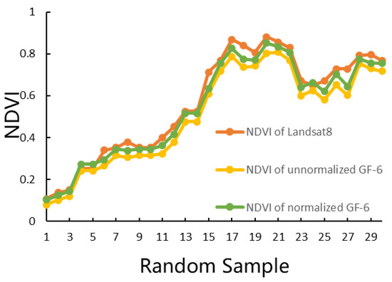
Figure 2.
Comparison between individual pixel values of Landsat-8 NDVI and normalized/unnormalized GF-6 NDVI images.
Table 3.
Statistical parameters of individual pixel values of Landsat-8 NDVI and normalized/unnormalized GF-6 NDVI.
2.2.3. Retrieval of Land Surface Temperatures (LSTs)
The single-channel algorithm [42] requires very few parameters to estimate LST, and is applicable in a certain range of atmospheric water vapor content, due to which, when high, the error of related parameters in the derivation process will increase, thus reducing the inversion accuracy. Conversely, when the atmospheric water vapor content decreases to 2 g∙cm−2, the retrieval error of LST decreases to between 1.53 K [43,44]. In this study, the atmospheric water vapor content was less than 2 g∙cm−2; the single-channel algorithm was, therefore, used to retrieve LST for the study area. Landsat-8 TIRS and GF-6 WFV, which after cross-radiation calibration replaced Landsat-8 OLI, were used to retrieve LST. For convenience, the 30-m Landsat-8 images and 16 m GF-6 images were both resampled into 100 m images. Furthermore, the 16 m GF-6 images were also resampled into 30 m images; 100 m and 30 m LST can be retrieved with TIRS. The 100 m-retrieved LSTs were the original LSTs for downscaling, and the 30 m-retrieved LSTs were used to evaluate downscaling results.
The governing equation of the single-channel algorithm is as follows:
where ε is surface emissivity, L is the radiant intensity measured by the remote sensing sensor at the altitude of the satellite (W∙m−2∙sr−1∙μm−1), T is the brightness temperature, λ is the central wavelength (band 10 of Landsat-8 has a central wavelength of 10.9 μm), c1 = 1.91104 × 10⁸ W∙μm4∙m−2∙sr−1 and c2 = 14,387.7 μm∙K, ψ1, ψ2, and ψ3 are atmospheric functional parameter, ω is the atmospheric water vapor content, is the absolute vapor pressure (hPa), RH is relative humidity, and T0 is air temperature measured at 2 m above the surface. RH and T0 are meteorological data of the Jinghe County meteorological station (ID:51334), which were downloaded from the China Meteorological Data Service Centre (http://data.cma.cn, accessed on 12 March 2022).
2.3. Three Classic LST Downscaling Methods Used
GF-6 and Landsat-8 TIRS images were first scaled up to 100 m to obtain the remote sensing index and original LST under the low resolution, and to establish the downscaling model. GF-6 images with original resolution were used to construct a high resolution of the remote sensing index to downscale the original LST.
2.3.1. DisTrad
The DisTrad method was first proposed by Kustas et al. in 2003. Based on the statistical law of scale invariance between NDVI and LST at different scales, Kustas achieved scaling down the thermal infrared image from 1 km to 100 m. The governing equation of DisTrad is as follows:
where LSTL is the LST value at the original resolution, is the simulated LST value at the coarser resolution, NDVIL is the NDVI value at the coarser resolution, a and b are constants, is the regression residual, NDVIH is the NDVI value at the finer resolution, and is the downscaled result.
2.3.2. TsHARP
The TsHARP method is an improved algorithm proposed by Agam [19] on the basis of the DisTrad algorithm. This method assumes that a relatively stable functional relationship between NDVI (or vegetation coverage) and LST is maintained at different spatial scales. In this method, a function between LST and NDVI is constructed at the coarser resolution, and this is then applied to the higher spatial resolution. Residual correction is then conducted to obtain the LST at the required resolution. The governing equation of the TsHARP method is as follows:
where f is the regression function between NDVI and Ts, ∆T is the regression residual, and a0 and a1 are the regression coefficients.
2.3.3. MIRF
Considering that the LST is affected by multiple factors, Yang et al. [20] proposed the MIRF algorithm. In MIRF, a downscaling model is constructed using random forest regression based on multiple surface-related remote sensing indices, which include the soil-adjusted vegetation index (SAVI), normalized multi-band drought index (NMDI), modified normalized difference water index (MNDWI), normalized difference dust index (NDDI), and the normalized difference building index (NDBI). The governing equation of MIRF is as follows:
in which SAVIL, NMDIL, NDBIL, MNDWIL, and NDDIL are the SAVI, NMDI, NDBI, MNDWI, and NDDI values at the coarser resolution, respectively, e is the regression residual, LSTO is the LST at the original resolution, LSTF is the simulated LST at the coarser resolution, SAVIH, NMDIH, NDBIH, MNDWIH, and NDDIH are the SAVI, NMDI, NDBI, MNDWI, and NDDI values at the finer resolution, respectively, and LSTH is the value of the downscaled LST.
2.4. Remote Sensing Indices Based on GF-6 Images
According to the field investigation and the GF-6 image of the study area, the underlying surface types of the study area mainly include vegetation, water bodies, impermeable surfaces, and barren soil. The remote sensing indices relating to these underlying surface types were selected. As NDDI cannot distinguish sand from soil, this indicator negatively affects the accuracy of LST downscaling, and it was, therefore, replaced by the normalized difference sand index (NDSI). Furthermore, as the GF-6 images does not provide shortwave infrared bands that can be used to compute the NDBI, which makes it difficult to identify built-up land using a single band or combination of bands, the ratio built-up index (RBI) was used instead of the NDBI [45]. Finally, based on underlying surface characteristics of the study area and the available bands of the GF-6 images, MIRF regression was conducted using the GF-6 NDVI, NDWI, RBI, and NDSI indices. To highlight the effects of the red-edge band 1 (RE1) and red-edge band 2 (RE2) on LST downscaling, three different NDVIs (NDVIGF6_Nir, NDVIRE1, and NDVIRE2) were constructed based on the common bands and RE1 and RE2 bands of the GF-6 image, and the equations used to compute each of these indices are as follows:
where ρNir and ρred are the reflectance values of the NIR and red bands, is the NDVI based on Nir band, ρver1 is the reflectance of RE1, NDVIRE1 is the NDVI based on RE1, ρver2 is the reflectance of RE2, and NDVIRE2 is the NDVI based on RE2.
where ρgreen and ρNir are the reflectance values of the green and NIR bands, respectively.
where ρblue, ρgreen, ρred, and ρNir are the reflectance values of the blue, green, red, and NIR bands, respectively.
Furthermore, the NDSI equation is as follows:
where ρred and ρblue are the reflectance values of the red and blue bands, respectively.
2.5. Evaluation Measures
Two measures were selected to evaluate the LST downscaling results, including R2 and RMSD, which were calculated as follows:
where is the downscaled result, is the reference LST, is the mean reference LST, and n is the total number of pixels in the image.
R2 is the coefficient of determination between the reference and downscaled images. RMSD was used to test the difference between the reference and downscaled LSTs. A high R2 and a low RMSD indicates a satisfactory downscaling. The Landsat-8- and GF-6-retrieved LSTs were used to evaluate the downscaling results of the resampling to 30 m.
3. Results
3.1. Evaluation of Downscaling Results
3.1.1. Downscaling Results
According to the field investigation and classification of GF-6 images in the study area, as compared with other regions, region A (Figure 3) contains all four types of underlying surfaces (vegetation, water bodies, impermeable surfaces, and barren soil), and their distribution is concentrated; Figure 4 shows an enlarged view of region A to present the downscaling results more clearly. Figure 5 shows the underlying surface types classified by GF-6 image, using support vector machines (SVM), with classification accuracies of 92.7%, 92.5%, and 94.4%. Figure 6 shows the Landsat-8- and GF-6-retrieved LST of region A, where a, b, and c show the original 100 m LSTs for downscaling, which were retrieved by GF-6 and Landsat-8 images scaled up to 100 m, and d, e, and f show the 30 m LSTs used to evaluate downscaling results, which were retrieved by GF-6 images resampled to the resolution of 30 m and the 30 m Landsat-8 TIRS images.
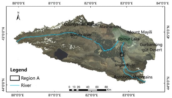
Figure 3.
The location of region A.
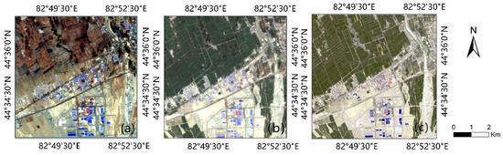
Figure 4.
Color composite of GF-6 images of region A (RGB:3, 2, 1) (a) 9 April 2019, (b) 24 July 2019, (c) 26 August 2019.

Figure 5.
Underlying surface types of region A (a) 9 April 2019, (b) 24 July 2019, (c) 26 August 2019.
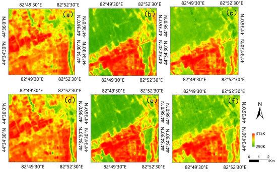
Figure 6.
Landsat-8- and GF-6-retrieved LST of region A (a) 100 m LST on 9 April 2019, (b) 100 m LST on 24 July 2019, (c) 100 m LST on 26 August 2019, (d) 30 m LST on 9 April 2019, (e) 30 m LST on 24 July 2019, (f) 30 m LST on 26 August 2019.
Figure 7 shows the 16 m downscaled LST taking 26 August 2019 as an example. As shown in Figure 7, all of the nine downscaled results in the three seasons were consistent with the overall spatial patterns of Landsat-8- and GF-6-retrieved LST, and their high- and low-temperature zones were general consistence with the Landsat-8- and GF-6-retrieved LST. Based on the images and underlying surface types of this region (Figure 5), barren soils had the highest temperatures, followed by impermeable surfaces. Vegetation had significantly lower temperatures than barren soil and impermeable surfaces, while water bodies had the lowest temperatures. This is consistent with the regular pattern that the temperature increases in water, vegetation, impervious surface, and poor soil. Comparing the DisTrad and TsHARP results, those based on NDVIGF6_Nir and NDVIRE2 were relatively similar to each other, but there were obvious changes in LST in vegetated areas which were obtained with the RE1 band changes. Compared to the Landsat-8- and GF-6-retrieved LST, the DisTrad- and TsHARP-downscaled results provided no additional details of LST variations. The MIRF-downscaled results from the common bands and the RE1 and RE2 bands of GF-6 can describe the detail spatial variations in LST. The temperature variations of the MIRF-downscaled results were also much milder.
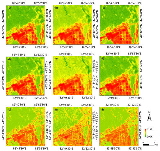
Figure 7.
The 16 m downscaled LSTs obtained using three different methods with GF-6 images of 26 August 2019. (a) DisTrad , (b) DisTrad , (c) DisTrad , (d) TsHARP , (e) TsHARP , (f) TsHARP , (g) MIRF , (h) MIRF , (i) MIRF .
The spatial distribution of the differences between Landsat-8- and GF-6-retrieved LST and downscaled LST (resampled to 30 m) shows that the temperature in the vegetation area was overestimated by each downscaling methods with RE1 band, and the range of overestimation gradually decreased with the order of DisTrad, TsHARP, and MIRF, as shown in Figure 8 (taking 26 August 2019 as an example). In the MIRF method, the temperature of impervious surface around vegetation and water covered area was higher, and the temperature of vegetation area in the middle of impervious surface and bare soil covered area were lower. The MIRF-downscaled LST results also revealed roads between vegetated areas, impermeable surfaces around water bodies, greenified areas among built-up areas, and temperature changes between impermeable and barren soil surfaces. These small temperature variations were absent from the Landsat-8- and GF-6-retrieved LST. Furthermore, the LST variations obtained by MIRF downscaling with the contribution of GF-6 images were consistent with the natural LST variations.
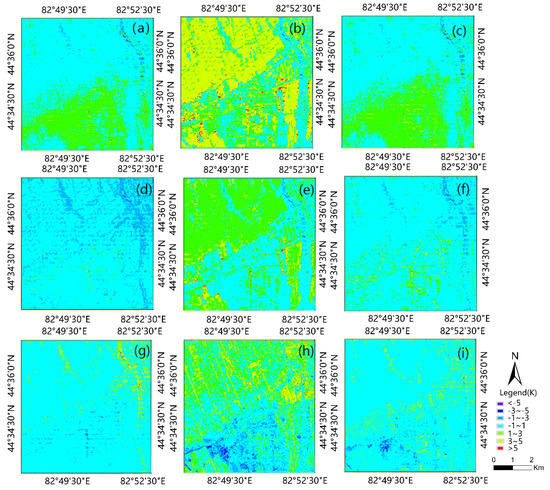
Figure 8.
Spatial distribution of the differences between the Landsat-8- and GF-6-retrieved LST dataset and downscaled results obtained using three different downscaling methods with different GF-6 bands on 26 August 2019 (in units of K). (a) DisTrad , (b) DisTrad , (c) DisTrad , (d) TsHARP , (e) TsHARP , (f) TsHARP , (g) MIRF , (h) MIRF , (i) MIRF .
3.1.2. Evaluation and Comparison of Downscaled LST
To evaluate the three methods, DisTrad, TsHARP, and MIRF, the downscaling results were scaled up to 30 m to be consistent with the Landsat-8- and GF-6-retrieved LST, the scatter plot of the downscaled results (from the common bands and two red-edge bands of GF-6), and the R2 and RMSD values of the downscaled results were calculated, as shown in Figure 9 (taking 26 August as an example) Statistical difference was evaluated between the downscaling results and Landsat-8- and GF-6-retrieved LSTs, as shown in Figure 10 (taking 26 August 2019 as an example). The statistics for all three groups are listed in Table 4.
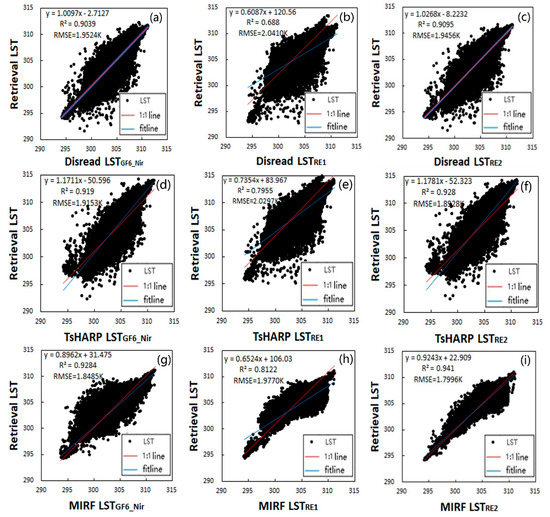
Figure 9.
Scatter plot of the Landsat-8- and GF-6-retrieved LST dataset and downscaled results obtained using three different downscaling methods with different GF-6 bands on 26 August 2019 (in units of K). (a) DisTrad , (b) DisTrad , (c) DisTrad , (d) TsHARP , (e) TsHARP , (f) TsHARP , (g) MIRF , (h) MIRF , (i) MIRF .
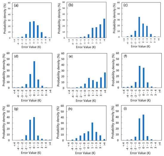
Figure 10.
Differences probability (with respect to Landsat-8- and GF-6-retrieved LST) in downscaled results obtained using three different downscaling methods and different GF-6 bands on 26 August 2019 (a) DisTrad , (b) DisTrad , (c) DisTrad , (d) TsHARP , (e) TsHARP , (f) TsHARP , (g) MIRF , (h) MIRF , (i) MIRF .
Table 4.
The statistics for the three groups.
It can be seen from Figure 9 and Figure 10 and Table 4 that the evaluation results that the three groups of images show consistent regular (Table 4). In a horizontal comparison between the downscaled results obtained with the same downscaling method but based on different NDVIs, downscaling with NDVIRE2 yielded the highest R2, the lowest RMSD values, and the largest number of pixels with residuals between −1 K and +1 K. Therefore, NDVIRE2 provided the optimal downscaling precision level. In the vertical comparison between the downscaled results with the same NDVI and different downscaling methods, MIRF-downscaled results consistently provided the highest R2, lowest RMSD, and the highest number of pixels with residuals between −1 K and +1 K.
Due to the cost of ground temperature observation equipment, there are limited observation station in the study area; therefore, the observation data were used as a supplement to evaluate the downscaling results.
Table 5 shows that the bias of retrieval LST at the three stations were all within 2.42 K, by comparing the three downscaling methods, it can be seen that the bias of DisTrad method at three stations were all within 3.95 K, TsHARP method within 3.47 K, and MIRF method within 1.96 K. Meanwhile, by comparing the downscaling results of three NDVIs, the bias of downscaling results with GF-6 NDVI at the three stations were all within 3.70 K, GF-6 NDVIRE1 was all within 3.95 K, and GF-6 NDVIRE2 was within 3.04 K. By comparing the downscaling results of the three seasons, the bias of downscaling results at three stations on the 9 April, 24 July, and 26 August 2019 were within 2.95 K, 2.76 K, and 3.95 K, respectively. MIRF LSTRE2 improved the accuracy of LST at all stations.
Table 5.
Bias of downscaling results and ground observation data (in K).
Therefore, MIRF was considered to be the most precise downscaling method and the optimal downscaling regression kernel was NDVIRE2, which provided additional spatial details.
3.2. Effects of the RE1 and RE2 Bands on LST Downscaling
The MIRF-downscaled results were used to analyze the effects of the new RE1 and RE2 bands on LST downscaling. A scatter plot was drawn using downscaled LSTs based on three different NDVIs (Figure 11), where it is evident that NDVI and LST have a “triangle-like” relationship that varies between the dry and wet edges; NDVI and LST are negatively correlated at the dry edges but positively correlated at the wet edges. Compared with NDVIGF6_Nir and NDVIRE2, the value of NDVIRE1 is lower at dry edge resulting in a higher value of the corresponding LST, the value of NDVIRE1 is higher at wet edge resulting in a lower value of the corresponding LST. The correlation coefficients of NDVIGF6_Nir, NDVIRE1, and NDVIRE2 with respect to LST were −0.85, −0.77, and −0.87 on 9 April 2019, the correlation coefficients of NDVIGF6_Nir, NDVIRE1, and NDVIRE2 with respect to LST were −0.93, −0.89, and −0.94 on 24 July 2019, and the correlation coefficients of NDVIGF6_Nir, NDVIRE1, and NDVIRE2 with respect to LST were −0.89, −0.86, and −0.91 on 26 August 2019, respectively. Therefore, NDVIRE2 correlated the most strongly (and negatively) with LST, and it is, thus, the most useful regression kernel for LST downscaling.
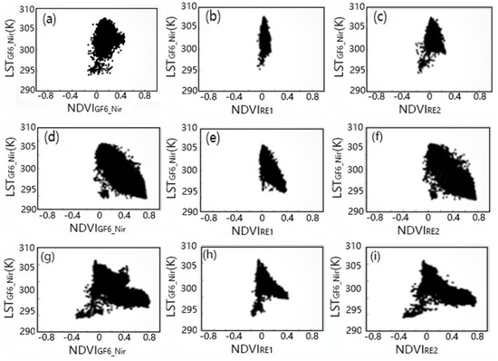
Figure 11.
Scatter distribution of three NDVI and the corresponding LST. (a) NDVIGF-6_Nir and LST on 9 April 2019, (b) NDVIRE1 and LST on 9 April 2019, (c) NDVIRE2 and LST on 9 April 2019, (d) NDVIGF-6_Nir and LST on 24 July 2019, (e) NDVIRE1 and LST on 24 July 2019, (f) NDVIRE2 and LST on 24 July 2019, (g) NDVIGF-6_Nir and LST on 26 August 2019, (h) NDVIRE1 and LST on 26 August 2019, (i) NDVIRE2 and LST on 26 August 2019.
4. Discussion
In this study, GF-6 and Landsat-8 images were used for downscaling experiments. The verification results indicate that the downscaled LST using the MIRF method and the regression kernel with GF6 RE2 band were generally accurate.
From the results of validation, the LST downscaling experiment (Figure 7) showed that all the downscaled results preserved the quality of the overall spatial pattern of Landsat-8- and GF-6-retrieved LST, while the high- and low-temperature zones were generally consistent with the regular pattern of nature compared to the MIRF. The DisTrad- and TsHARP-downscaled results provided no additional details regarding LST variations. The MIRF-downscaled results reflect the spatial distribution details of LST on a small scale for detecting temperature changes between roads covered by vegetation, impervious surfaces around water bodies, green areas in urban construction areas, and impervious surfaces and bare soil. These detailed differences are absent in the Landsat-8- and GF-6-retrieved LST. The spatial distribution of the differences between Landsat-8- and GF-6-retrieved LST and downscaled LST (Figure 8) showed that the temperature in the vegetation area was all overestimated by each downscaling methods with RE1 band, and the range of overestimation gradually de-creased with the order of DisTrad, TsHARP, and MIRF. From the quantitative results, as shown in Figure 9 and Table 4, as compared with the Landsat-8- and GF-6-retrieved LST, the variation degree of the downscaling results was different. Upon comparing the downscaled results obtained for different NDVIs, downscaled with NDVIRE2 yielded the highest R2, with the lowest RMSD values among all downscaling methods. Moreover, upon comparison between the results of different downscaling methods, the MIRF-downscaled results provided the highest R2, while the lowest RMSD for all NDVIs. This suggests that the downscaling results of NDVIRE2 using MIRF had the highest accuracy and the lowest scaling effect.
As shown in Figure 10, the distribution of differences is left-skewed in each method using NDVIRE1. Therefore, the results of the three NDVI participations versions in the MIRF method were further analyzed, as shown in Figure 11. Compared with NDVIGF6_Nir and NDVIRE1, the value of NDVIRE1 is lower at dry edge resulting in a higher value of the corresponding LST, the value of NDVIRE1 is higher at wet edge resulting in a lower value of the corresponding LST. This is related to the central wavelength of band RE1, which is 710 μm, and the vegetation condition of the study area. The reflectivity of vegetation increases sharply, which is reflected by the steep slope, from visible band to the spectral region of approximately 710 μm [46,47]. NDVIRE2 had a stronger negative correlation with LST, while NDVIRE1 has the lowest correlation, which were consistent with those shown in Figure 9. The spatial distribution of land surface temperature was correlated with the spatial distribution of landscape features of underlying surface. In this study, we introduced NDVIRE2 into three typical algorithms instead of NDVIGF6_Nir, and obtained the most satisfactory downscaling LST results with MIRF. Thus, the four remote sensing indices selected in this experiment can better express the surface features of the study area, which is helpful to improve the accuracy of LST downscaling.
We discussed the feasibility and accuracy of using GF-6 WFV images and statistical models to perform LST downscaling of the study area in this paper. High-spatial resolution LST contains more abundant textural information and can effectively reflect the surface temperature in terms of small-scale spatial heterogeneity. It would be helpful to further study the causes and characteristics of heat island effect in the study area, and the results can aid in agricultural irrigation, regional planning, drought assessment, ecological monitoring, water-heat balance research, and water resources allocation. Based on the analysis of the high-resolution spatial distribution of LST and its driving factors, a high-resolution geospatial resilience map can be drawn, which is critical for understanding the complex interactions between human (socioeconomic) and natural (ecological) systems. Evaluation of these systems is essential for determining sustainable development policies for the study area.
The errors in geometric correction between different source images leads to errors in the experimental results. Hence, further studies are needed regarding the influence of using GF-6 to construct other remote sensing indexes as regression kernels on LST downscaling. Based on the 16 m LST obtained in this study, we show that GF6 PMS images can be used to conduct research at higher spatial resolutions. Further research is needed to understand the effect of the superiority of GF-6 red-edge bands in vegetation recognition ability on downscaling results.
5. Conclusions
A preliminary study was conducted on the feasibility of using GF-6 images for LST downscaling in the Ebinur Lake Watershed. Landsat-8- and GF-6 WFV images obtained during the growing season (spring, summer, and autumn) were used as data sources, downscaling model was constructed, and the selection of regression kernel was explored in this study. The following conclusions were obtained by comparison analysis:
- (1)
- Compared with Landsat-8- and GF-6-retrieved LST, the results of downscaling LST using NDVIRE2 as a single factor regression kernel had the highest R2 and the lowest RMSD, and the number of pixels with LST errors of between −1 K and +1 K were the highest. As NDVIRE2 was strongly and negatively correlated with the downscaled LSTs, it might be an excellent indicator of the spatial variations in LSTs and provide an outstanding LST downscaling performance.
- (2)
- The downscaling method of multi-remote sensing indices is better than the single-factor method; the correlation between LST and NDVI is not obvious in the high heterogeneity area, which causes to a large error in the downscaling results of the single-factor method. The spatial patterns of downscaled LSTs using NDVIRE2, RBI, NDSI, and NDWI as multi-remote sensing indices with the MIRF method were consistent with the Landsat-8- and GF-6-retrieved LST, which improved the accuracy of LST at all stations; hence, the downscaled LSTs provide additional details spatial description of LST variations, which were absent in Landsat-8- and GF-6-retrieved LSTs. Furthermore, the temperature gradations of the downscaled LSTs were smoother and more consistent with the natural variations in LST.
- (3)
- The results of this study prove the viability of downscaling LSTs based on GF-6 and Landsat-8 images. Furthermore, 16 m-resolution images were successfully used to improve the medium-resolution LST. The downscaling results also proved to be reliable and highly precise, and can meet the application requirements of LST spatial resolution in the study area.
Author Contributions
Conceptualization, X.H.; methodology, X.L. and X.P.; experiments, X.L.; investigation, X.L. writing—original draft preparation, X.L.; suggestions, X.H. and X.P. All authors have read and agreed to the published version of the manuscript.
Funding
This research received funding supported by the National Natural Science Foundation of China (No. 41830110 and No. 41701487), Fundamental Research Funds for the Central Universities (No. 2019B02714), and National High Resolution Earth Observation System Major Project (No. 95-Y20A10-9001-16/17).
Acknowledgments
We express our sincere gratitude to the Satellite Application Center of Xinjiang Uygur Autonomous Region and the Hydrographic and Water Resources Survey Bureau of Xinjiang Bortala Mongolia Autonomous Prefecture for the remote sensing images and ground measurement data provided for this study, without which this study would have been impossible.
Conflicts of Interest
The authors declare no conflict of interest.
References
- Dewan, A.G.K.; Botje, D.D.; Mahmud, G.I.; Bhuian, H.M.; Hassan, Q.K. Surface urban heat island intensity in five major cities of Bangladesh: Patterns, drivers and trends. Sustain. Cities Soc. 2021, 71, 102926. [Google Scholar] [CrossRef]
- Chakraborty, T.A.H.; Manya, D.; Sheriff, G. A spatially explicit surface urban heat island database for the United States: Characterization, uncertainties, and possible applications. ISPRS J. Photogramm. Remote Sens. 2020, 168, 74–88. [Google Scholar] [CrossRef]
- Quattrochi, D.A.; Luvall, J.C. Thermal Remote Sensing in Land Surface Processes, 1st ed.; CRC Press: Boca Raton, FL, USA, 2003. [Google Scholar]
- Xiaoyan, D. A Study on Land Surface Temperature Retrieval over Urbanized Region Based on Remote Sensing Data Mining; East China Normal University: Shanghai, China, 2008. [Google Scholar]
- Shaohua, Z.; Qiming, Q.; Feng, Z.; Qiao, W.; Yunjun, Y.; Lin, Y.; Hongbo, J.; Rongbo, C.; Yanjuan, Y. Research on Using a Mono-Window Algorithm for Land Surface Temperature Retrieval from Chinese Satellite for Environment and Natural Disaster Monitoring(HJ-1B) data. Spectrosc. Spect. Anal. 2011, 31, 1552–1556. [Google Scholar] [CrossRef]
- Tomlinson, C.J.; Chapman, L.; Thornes, J.E.; Baker, C. Remote sensing land surface temperature for meteorology and climatology: A review. Meteorol. Appl. 2011, 18, 296–306. [Google Scholar] [CrossRef] [Green Version]
- Gong, P.; Li, X.; Wang, J.; Bai, Y.; Zhou, Y. Annual maps of global artificial impervious area (GAIA) between 1985 and 2018. Remote Sens. Environ. 2019, 236, 111510. [Google Scholar] [CrossRef]
- Girardet, H. People and Nature in an Urban World. One Earth 2020, 2, 135–137. [Google Scholar] [CrossRef] [Green Version]
- Tzu-Ling Chen, Z.-H.L. Impact of land use types on the spatial heterogeneity of extreme heat environments in a metropolitan area. Sustain. Cities Soc. 2021, 72, 103005. [Google Scholar] [CrossRef]
- Oni, S.B.A.; Anniballe, R.; Pierdicca, N. Downscaling of the land surface temperature over urban area using Landsat data. In Proceedings of the IGARSS, Milan, Italy, 26–31 July 2015; pp. 1144–1147. [Google Scholar] [CrossRef]
- Yiran, Z. Research on Disaggregation of Land Surface Temperature and Its Application in GF-1/GF-2 Image; Zhejiang University: Hangzhou, China, 2017. [Google Scholar]
- Liu, B.; Zhang, Y.S. Retrieval and Analysis of Downscaling Land Surface Temperature Based on Landsat-8 and ZY-3 Satellite Imafery. Remote Sens. Infotm. 2018, 33, 28–34. [Google Scholar] [CrossRef]
- Lijuan, Z. Crop Classification Using Multi-Features of Chinese Gaofen-1/6 Satellite Remote Sensing Images; University of Chinese Academy of Sciences: Beijing, China; Institute of Remote Sensing and Digital Earth, Chinese Academy of Sciences: Beijing, China, 2017. [Google Scholar]
- Ji, L.; Zhenwei, Z.; Shiting, X.; Xiaotong, Z.; Yuanyuan, T. Crop recognition and evaluation using red edge features of GF-6 satellite. J. Remote Sens. 2020, 24, 1168–1179. [Google Scholar] [CrossRef]
- Liang, Z.Z.; Sui, A.; Yu, Y.; Zhao, G. Rapid Identification of Forestland with GF6 Data. J. Northeast For. Univ. 2020, 48, 35–39. [Google Scholar] [CrossRef]
- Changdong, K.Z. Comparative Study on the Extraction Methods of the Built-up Areas of GF-6. Laser Optoelectron. Prog. 2021, 4, 439–446. [Google Scholar] [CrossRef]
- Jinling, Q.Z.W.; Yunhao, C.; Wenyu, L. Downscaling remotely sensed land surface temperatures: A comparison of typical methods. J. Remote Sens. 2013, 17, 374–387. [Google Scholar] [CrossRef]
- Kustas, W.P.; Norman, J.M.; Anderson, M.C.; French, A.N. Estimating subpixel surface temperatures and energy fluxes from the vegetation index–radiometric temperature relationship. Remote Sens. Environ. 2003, 85, 429–440. [Google Scholar] [CrossRef]
- Agam, N.; Kustas, W.P.; Anderson, M.C.; Li, F.; Neale, C.M.U. A vegetation index-based technique for spatial sharpening of thermal imagery. Remote Sens. Environ. 2007, 107, 545–558. [Google Scholar] [CrossRef]
- Yang, Y.; Chen, C.; Xin, P.; Li, X.; Xi, Z. Downscaling Land Surface Temperature in an Arid Area by Using Multiple Remote Sensing Indices with Random Forest Regression. Remote Sens. 2017, 9, 789. [Google Scholar] [CrossRef] [Green Version]
- Xin, P.; Xi, Z.; Yang, Y.; Chen, C.; Zhang, X.; Shan, L. Applicability of Downscaling Land Surface Temperature by Using Normalized Difference Sand Index. Sci. Rep. 2018, 8, 9530. [Google Scholar] [CrossRef] [Green Version]
- Yang, Y.; Li, X.; Pan, X.; Zhang, Y.; Cao, C. Downscaling Land Surface Temperature in Complex Regions by Using Multiple Scale Factors with Adaptive Thresholds. Sensors 2017, 17, 744. [Google Scholar] [CrossRef] [Green Version]
- Chen, C. Downscaling Multi-resolution Landsurface Temperature Research. Mod. Surv. Mapp. 2018, 41, 3–8. [Google Scholar] [CrossRef]
- Wang, Y.; Liu, Z.; Yao, J.; Bayin, C. Effect of climate and land use change in Ebinur Lake Basin during the past five decades on hydrology and water resources. Water Resour. 2017, 44, 204–215. [Google Scholar] [CrossRef]
- Yuejian, W. Study on the Influence of the Change of Water Resourcesandits Impacton Ecological Security in th eArid: An Example of Ebinur Lake Basin in Xinjiang; Xinjiang University: Urumqi, China, 2018. [Google Scholar]
- Lin, K.; Mao, Y.; Hongbo, L.; Wenxia, T.; Yao, C. Analysis of regional climate change impact on surface runoff in Jinghe river in recent forty-eight years. J. Water Resour. Water Eng. 2013, 24, 54–59. [Google Scholar]
- Fei, Z.; Yibo, L. Analysis of distribution Patterns and Spatial Variality of Soil Salinity Affecting Factors in Topsoil Layer of Salinized Soil in Jinghe oasis. J. Ecol. Rural Environ. 2018, 34, 64–73. [Google Scholar] [CrossRef]
- Yibing, Q.; Zhaoning, W.; Liyun, Z.; Aili, Y. Ground-Surface Conditions of Sand-Dust Event Occurrence and Soil Conservation in Aibi Lake Region of Xinjiang. Resour. Sci. 2006, 28, 185–189. [Google Scholar] [CrossRef]
- Zhaopeng, W.; Mingxia, W.; Xiao, Z. The changes of desertification from 1990–2011 in Jinghe watershed. J. Arid Land Resour. Environ. 2015, 29, 192–197. [Google Scholar] [CrossRef]
- Yan, C. Relationship between Desert Plant Diversity and Ecosystem Multifunctionality along Water and Salt Gradients; Xinjiang University: Urumqi, China, 2019. [Google Scholar]
- Zhaopeng, W.; Sujuan, N.; Min, M.; Aimaiti, Y.; Jinyan, Z. Remote sensing research on the spatial-temporal pattern of” cold island effect” of oasis in Jinghe River basin. Remote Sens. Land Resour. 2020, 32, 106–113. [Google Scholar] [CrossRef]
- Lacerda, L.N.; Cohen, Y.; Snider, J.; Liakos, V.; Vellidis, G. Field Scale Assessment of the TsHARP Technique for Thermal Sharpening of MODIS Satellite Images Using VENS and Sentinel-2-Derived NDVI. Remote Sens. 2021, 13, 1155. [Google Scholar] [CrossRef]
- Yan, S. Study on the Relationship between Soil, Surface Temperature Characteristics and Landscape Pattern around the Ebinur Lake Wetland Edge; Xinjiang Normal University: Urumqi, China, 2016. [Google Scholar]
- Zhang, F.; Wang, J.; Tashpolat, T.; Zhou, M.; Li, X.H. The spatial and temporal dynamic changes and driving forces in the surface area of ebinur lake from 1998–2013. Acta Ecol. Sin. 2015, 35, 2848–2859. [Google Scholar] [CrossRef]
- Garnier, A.; Pennekamp, F.; Lemoine, M.; Petchey, O.L. Temporal scale dependent interactions between multiple environmental disturbances in microcosm ecosystems. Glob. Chang. Biol. 2017, 23, 5237–5248. [Google Scholar] [CrossRef] [Green Version]
- Ostrom, J.E. Resilience, vulnerability, and adaptation: A cross-cutting theme of the International Human Dimensions Programme on Global Environmental Change. Glob. Environ. Chang. 2006, 16, 237–239. [Google Scholar] [CrossRef]
- Nguyen, K.A.; Liou, Y.A. Global mapping of eco-environmental vulnerability from human and nature disturbances. Sci. Total Environ. 2019, 664, 995–1004. [Google Scholar] [CrossRef]
- Battamo, A.Y.; Varis, O.; Sun, P.; Yang, Y.; Oba, B.T.; Zhao, L. Mapping socio-ecological resilience along the seven economic corridors of the Belt and Road Initiative. J. Clean. Prod. 2021, 309, 127341. [Google Scholar] [CrossRef]
- Yang, A.; Zhong, B.; Lv, W.; Wu, S.; Liu, Q. Cross-Calibration of GF-1/WFV over a Desert Site Using Landsat-8/OLI Imagery and ZY-3/TLC Data. Remote Sens. 2015, 7, 10763–10787. [Google Scholar] [CrossRef] [Green Version]
- Aixia, Y. Researh on Method and System for Radiometric Cross-Calibration of China’s Optical Satellite Remote Sensing Data on VNIR Bands; University of Chinese Academy of Sciences: Beijing, China, 2017. [Google Scholar]
- Yang, A.; Zhong, B.; Hu, L.; Wu, S.; Xu, Z.; Wu, H.; Wu, J.; Gong, X.; Wang, H.; Liu, Q. Radiometric Cross-Calibration of the Wide Field View Camera Onboard GaoFen-6 in Multispectral Bands. Remote Sens. 2020, 12, 1037. [Google Scholar] [CrossRef] [Green Version]
- Jimenez-Munoz, J.C.; Cristobal, J.; Sobrino, J.A.; Soria, G.; Ninyerola, M.; Pons, X.; Pons, X. Revision of the Single-Channel Algorithm for Land Surface Temperature Retrieval From Landsat Thermal-Infrared Data. IEEE Trans. Geosci. Remote Sens. 2008, 47, 339–349. [Google Scholar] [CrossRef]
- Hanqiu, X. Retrieval of the reflectance and land surface temperature of the newly-launched Landsat 8 satellite. Geophysics 2015, 58, 741–747. [Google Scholar] [CrossRef]
- Ting, S.; Zheng, D.; Junzhi, L.; Junzhe, S.; Fei, Y.; Shijie, S.; Jun, H.; Wei, W. Comparison of four algorithms to retrieve land surface temperature using Landsat 8 satellite. J. Remote Sens. 2015, 19, 451–464. [Google Scholar] [CrossRef]
- Yang, W.Z.; Zhang, Y.J.; Yin, X.H.; Wang, J. Construction of ratio build-up index for GF-1 image. Remote Sens. Land Resour. 2016, 28, 35–42. [Google Scholar] [CrossRef]
- Horler, D.N.H.; Dockray, M.; Barber, J. The red edge of plant leaf reflectance. Int. J. Remote Sens. 1983, 4, 273–288. [Google Scholar] [CrossRef]
- Jianwen, H.; Erxue, L.Z.C.; Lei, Z.; Bingping, M. Classification of plantation types based on WFV multispectral imagery of the GF-6 satellite. J. Remote Sens. 2021, 25, 539–548. [Google Scholar] [CrossRef]
Publisher’s Note: MDPI stays neutral with regard to jurisdictional claims in published maps and institutional affiliations. |
© 2022 by the authors. Licensee MDPI, Basel, Switzerland. This article is an open access article distributed under the terms and conditions of the Creative Commons Attribution (CC BY) license (https://creativecommons.org/licenses/by/4.0/).