Article

Arctic Sea Ice Classification Based on CFOSAT SWIM Data at Multiple Small Incidence Angles

1
College of Physics, Qingdao University, Qingdao 266071, China
2
First Institute of Oceanography, Ministry of Natural Resources of China, Qingdao 266061, China
3
National Satellite Ocean Application Service, Beijing 100082, China
4
School of Electronics and Information Engineering, Huazhong University of Science and Technology, Wuhan 430074, China
*
Author to whom correspondence should be addressed.
Remote Sens. 2022, 14(1), 91; https://doi.org/10.3390/rs14010091
Submission received: 27 November 2021 / Revised: 19 December 2021 / Accepted: 21 December 2021 / Published: 25 December 2021
(This article belongs to the Special Issue Remote Sensing Monitoring of Arctic Environments)

Abstract

:
Sea ice type is the key parameter of Arctic sea ice monitoring. Microwave remote sensors with medium incidence and normal incidence modes are the primary detection methods for sea ice types. The Surface Wave Investigation and Monitoring instrument (SWIM) on the China-France Oceanography Satellite (CFOSAT) is a new type of sensor with a small incidence angle detection mode that is different from traditional remote sensors. The method of sea ice detection using SWIM data is also under development. The research reported here concerns ice classification using SWIM data in the Arctic from October 2019 to April 2020. Six waveform features are extracted from the SWIM echo data at small incidence angles, then the distinguishing capabilities of a single feature are analyzed using the Kolmogorov-Smirnov distance. The classifiers of the k-nearest neighbor and support vector machine are established and chosen based on single features. Moreover, sea ice classification based on multi-feature combinations is carried out using the chosen KNN classifier, and optimal combinations are developed. Compared with sea ice charts, the overall accuracy is up to 81% using the optimal classifier and a multi-feature combination at 2°. The results reveal that SWIM data can be used to classify sea water and sea ice types. Moreover, the optimal multi-feature combinations with the KNN method are applied to sea ice classification in the local regions. The classification results are analyzed using Sentinel-1 SAR images. In general, it is concluded that these multifeature combinations with the KNN method are effective in sea ice classification using SWIM data. Our work confirms the potential of sea ice classification based on the new SWIM sensor, and highlight the new sea ice monitoring technology and application of remote sensing at small incidence angles.

1. Introduction

Sea ice influences a number of important processes, such as the global radiation balance and the exchange of heat and momentum between the ocean and the atmosphere, and sea ice has a strong influence on regional climate, marine and coastal habitats in Arctic environments, as well as marine transport and other human activities in and near polar seas [1]. Sea ice extent clearly continues to exhibit a long-term downward trend over past years in the Arctic [2]. Therefore, long-term sea ice monitoring is an important operational task. Sea ice type is one of the key parameters to characterize the properties and variations of sea ice, and a wide variety of tools are commonly used, including observations from ships, buoys, aircraft, and satellites [3,4]. Space-borne microwave sensors have been used in various studies to classify sea ice types, such as first-year ice (FYI) or multiyear ice (MYI), surviving more than one melting summer season, and sea water (SW) [5,6,7].
Satellite-based microwave sensors mainly include synthetic aperture radar (SAR), altimeters and scatterometers. SAR is one type of imaging radar with medium incidence angles of 20° to 60° and high spatial resolution up to the submeter level. SAR monitors the local and regional sea ice distribution and variation for the recognition of sea ice types, sea ice condition assessment in important areas and fine navigation in the Arctic based on the abundant microwave backscattering information of sea ice. Sea ice classification has been performed for operational applications [8]. Moreover, sea ice types and sea water can be distinguished automatically with high accuracies of up to 95% [9,10,11].
An altimeter is mainly used for sea ice thickness retrieval using sea ice freeboard with a normal incidence mode based on large-scale and coarse spatial resolution (several to tens of kilometers) observations covering all polar regions. The ability to distinguish sea ice types can improve the conversion from freeboard to thickness. Waveform features are used in the recognition of sea ice types and sea water, such as backscattering power (BSP), maximum power (MAX), pulse peakiness (PP), leading edge width (LEW), trailing edge width (TEW), and stack standard deviation (SSD). Drinkwater and Carsey [12] distinguished sea ice with rough surfaces and smooth surfaces using waveform features derived from airborne Ku-band radar altimeters. For smooth sea ice, the waveform peak is higher, and the trailing edge descends more quickly. Zygmuntowska et al. [13] presented a Bayesian-based method to classify FYI and MYI using PP and TEW waveform features, and showed a classification accuracy of approximately 80%. Rinne and Similä [14] presented an automatic classification system for detecting sea water, thin FYI, thick FYI, and MYI using a K-nearest-neighbors (KNN) classifier based on recent ice charts for training and four CryoSat-2 PP, LEW, SSD, and late-tail-to-peak-power ratio (LTPP) waveform features; the accuracies were approximately 85%. Shen et al. [15] distinguished FYI from MYI using a random forest (RF) classifier based on six waveform features (TEW, LEW, σ0, MAX, PP and SSD), and the accuracy was 85%. Shen et al. [16] presented a systematic comparison of popular machine-learning classifiers with different feature combinations to find the optimal classifier–feature assembly, which was the RF accompanied by a feature combination of TEW, LEW, σ0, MAX, and PP; the result achieved a mean accuracy of 91%. Shu et al. [17] proposed an object-based random forest (ORF) classification method with a feature combination of σ0, MAX, PP and SSD, and the overall classification accuracy was up to 90%. Sea ice classification using altimeters is still being researched and is not used operationally.
Scatterometers at medium incidence angles (20° to 60°) can observe sea ice all over polar regions to recognize sea ice types and sea water with a similar resolution to altimeters, including two major frequencies: the C-band (e.g., ASCAT, ERS-1/2) and Ku-band (e.g., QuickSCAT, OSCAT). Sea ice classification methods using scatterometer data can be divided into two categories. One is based on the microwave backscattering characteristics of sea ice, including the backscattering powers of the horizontal and vertical polarization. Sea ice and sea water recognition was first carried out using C-band data [12,18,19], and then the Ku-band was demonstrated to be applicable for recognizing sea ice and sea water [20,21]. Recognition accuracies achieved 90% [22]. As a result, operational products of sea ice extent and concentration in the Arctic and Antarctic have been manufactured for a long time [23,24,25,26]. The distinction of sea ice types (e.g., FYI and MYI) followed [27,28]. The other classification method is scatterometer image reconstruction (SIR) method. The reconstruction image can acquire a higher spatial resolution based on the multi-incidence and multi-azimuth original data of C- and Ku-band scatterometers and is used to distinguish sea ice types and sea water using image recognition methods [4,29,30]. This operational method has been used to produce sea ice charts for nearly a decade, as proposed by Remund and Long [24].
Microwave remote sensors with small incidence angles have been used for observation. The dual-frequency precipitation radar (DPR) onboard the Global Precipitation Measurement (GPM) adopts small incidence angles of ±17° using Ku-bands and Ka-bands. The GPM orbit is circular and non-sun-synchronous with an inclination of 65 degrees. As a result, the observation region of DPR only covers latitudes between 66.3° N and 66.3° S, and the DPR cannot detect the main areas in the Arctic. The Chinese-French Oceanic Satellite (CFOSAT) was successfully launched on 29 October 2018 and was developed by the China National Space Administration (CNSA) and the Centre National D’Etudes Spatiales (CNES) [31,32]. CFOSAT, which is devoted to observing ocean surface wind and waves, carries two Ku-band radar payloads: the wave scatterometer (Surface Waves Investigation and Monitoring, SWIM) and the wind scatterometer (rotating fan-beam scatterometer, RFSACT) [33,34]. SWIM is the first space-borne instrument using a rotating six-beam radar comprised of a scanning-beam real aperture radar operating at 13.575 GHz at small incidence angles (0° to 10°) [35]. The main mission of SWIM is to obtain sea surface waves. RFSACT operating at 13.3 GHz, detects sea surface wind and sea ice properties with medium incidence angles (26° to 61°) [36]. Sea ice detection in the small incidence angle mode has rarely been studied thus far. Therefore, for a new detection mode of small incidence angles, several key problems should be studied in sea ice classification, such as the ability to recognize sea ice types and sea water, the performance of each small incidence angle in category discrimination, the selection and optimization of waveform features or waveform feature combinations and classifiers, the application of optimal multifeature combinations using selected classifiers, and the abilities of small, normal and medium-incidence sensors in sea ice classification. Therefore, our work focuses on the study of sea ice classification using the SWIM data at small incidence angles according to these problems, which can promote new sea ice detection technology and expand new horizons for SWIM ocean detection applications.
Section 2 describes the data sets of SWIM data, Sentinel-1 SAR images and sea ice charts in the Arctic from October 2019 to April 2020, and data processes including waveform feature extraction, data matching and filtering. Moreover, the analysis method of sea ice discrimination ability and sea ice classification methods are also introduced. Section 3 presents results of waveform analysis, sea ice discrimination ability, overall accuracies of different methods, and sea ice classification results using multi-feature combinations of SWIM data. Section 4 discusses the comparison with previous achievements, the recognition rate of sea water, the influence of snow coverage, the feasibility of new feature introduction, and the necessity of further similar studies. Section 5 presents the conclusions and an overview of future work.

2. Data and Method

2.1. Data

2.1.1. SWIM Data

CFOSAT is a joint mission that makes use of a polar orbit; its orbit characteristics are shown in Table 1. SWIM, as an innovative sensor with the main objective of providing directional wave spectra, and consists of a real aperture radar (RAR) operating in the Ku-band (13.575 GHz) with six distinct beams pointing at small incidence angles from 0° (nadir) to 10° while scanning the whole azimuth angle (0–360°). The SWIM swath is nearly 90 km from nadir to the outer edge of the footprint at 10°. The footprint at 10° is approximately 18 km. The number of bins with different incidence angles is large, and larger than the number of the RFSCAT. The geometry and resolution parameters are shown in Figure 1 and Table 2. SWIM data were processed to three levels, L1A, L1B and L2; the L1A level data include echo waveforms, which can be used to extract waveform features and recognize sea ice types and sea water in this study.

2.1.2. Sentinal-1 SAR

Sentinel-1 is the first of five missions developed for the Copernicus initiative of the European Commission (EC) and the European Space Agency (ESA). The mission is designed as a two-satellite constellation, which was launched on 3 April 2014 for Sentinel-1A and 25 April 2016 for Sentinel-1B. Sentinel-1A/B carries advanced imaging radars to provide continuous all-weather, day-and-night data. Sentinel-1A/B operates at the C-band in single polarisation (HH or VV) and dual polarisation (HH+HV or VV+VH). The Sentinel-1A/B synthetic aperture radar (SAR) operates in four exclusive modes: stripmap (SM) mode, interferometric wide swath (IW), extra-wide swath (EW) and wave (WV), and provides four products: Level-0 data, Level-1 Single Look Complex (SLC), Level-1 Ground Range Detected (GRD) and Level-2 Ocean (OCN).
Sentinel-1A/B can support high-resolution ice charting services; for example, the detection of changes in the Arctic sea ice extent and sea ice classification. Moreover, beyond supporting operational services, Sentinel-1A/B exhibits enhanced capabilities for short and long-term variables of ice sheets, such as the motion of ice masses [37]. GRD images in IW and EW modes are used in this study.

2.1.3. Sea Ice Chart

Sea ice charts for sea ice classification and the evaluation of the results are from the Arctic and Antarctic Research Institute (AARI) of the State Scientific Center of the Russian Federation, which belongs to the Russian Federal Service on Hydrometeorology and Environmental Protection [38].
The AARI collects data (averaging) for the preceding two to five day intervals, which is usually from every Sunday to Tuesday, and then issues sea ice charts every Thursday. Sea ice charts are based on a generalization of regional ice charts compiled from the analysis of satellite (visible, infrared and radar) information and reports from coastal stations and ships. Sea ice charts are divided into two periods. One is the winter period when the charts show the generalized distribution of sea ice development stages (ice thickness) including nilas, young, FYI and MYI, and the other is the summer period when the charts express generalized distribution of the categories of sea ice total concentration for intervals of 1–6/10 s and 7–10/10 s [38]. As shown in Table 3, there are 31 sea ice charts in the Arctic from October 2019 to April 2020.
An Arctic ice year is from October to April. The main sea ice categories include nilas (thickness <10 cm), young ice (<30 cm), first-year ice (<2 m), multiyear ice, and sea water. Nilas and young ice appear in October, develop rapidly in October and November, and decrease in December. The two types stabilize to a very small extent starting in January. Nilas and young ice exhibit similar growth properties and approximate thicknesses. Therefore, these two types of sea ice merge into thin ice (TI). Thus, there are four categories in this study based on the AARI sea ice charts: thin ice (TI), first-year ice (FYI), multiyear ice (MYI), and sea water (SW).

2.1.4. Extraction of SWIM Waveform Features

Six waveform features are extracted to describe the echo waveform characteristics of SWIM at the six small incidence angles. SWIM does not provide automatic gain control (AGC). Thus, the SWIM data are not further processed by AGC. These features are:
(1)
Maximum power (MAX)
MAX is the maximum value of the waveform power, which can reflect the surface characteristics [39]. MAX is expressed by the following formula:
P max θ =   max ( P i θ ) ,   i θ = 1 ,   2 ,   3 ,   ,   n θ ,   unit :   W
where P i θ is the power in the i-th range bin of the incidence angle θ and nθ is the maximum range bin of the incidence angle θ, that is, nθ = 256, 765, 933, 2771, 2639, 3215, for the incidents θ = 0°, 2°, 4°, 6°, 8°, 10°, respectively.
(2)
Backscattering power (BSP)
BSP is the fundamental parameter in previous research on sea ice classification and is sensitive to the surface characteristics of sea ice and sea water. The BSP is a function of the radar frequency, polarization and incidence angle, and is related to the surface roughness, geometry and dielectric property of the object. Its unit is W. The BSP of one footprint is calculated using the offset center of gravity at an incidence angle of 0° [40]:
BSP θ = i = 1 n θ P i θ 4 i = 1 n θ P i θ 2 ,   θ   = 0 ° .
The BSP is the average value of one waveform at an incidence angle of 2°–10°:
BSP θ = i = 1 n θ P i θ n θ ,   θ   = 2 ° ,   4 ° ,   6 ° ,   8 ° ,   10 ° .  
(3)
Pulse peakiness (PP)
PP, proposed by [41], expresses the specular return of echo waveforms, that is, large PP with high reflectance in the smooth surface at 0° [13], and it may be in contrast at larger incidence angles. PP is defined by the ratio of MAX to the accumulated echo power:
P P θ = P max θ i θ = 1 n θ P i θ × n θ  
(4)
Stack standard deviation (SSD)
SSD is the standard deviation of the power values from a common surface formed from a set of Doppler waveforms at different incidence angles [42].
SSD = i θ = 1 n θ ( P i θ P ¯ θ ) 2 n θ , P ¯ θ = i θ = 1 n θ P i θ n θ , unit : W
where P ¯ θ is the mean power at the incidence angle θ. The standard deviation expresses the dispersion and stability of the waveform power.
(5)
Leading edge width (LEW)
LEW is the distance between the corresponding bins at 5% and 95% of the maximum power echo of the leading edge, resulting in filtering out of the influence of the leading thermal noise. LEW is smaller in specular reflection than in diffuse reflection at 0°, and it may be different at larger incidence angles.
A 1 θ =   P max θ · 0 . 95 ,   A 2 θ =   P max θ · 0 . 05 ,   LEW = Bin ( A 1 θ ) Bin ( A 2 θ )
where Bin(*) represents the bin at the incidence angle θ corresponding to the value of ‘*’.
(6)
Trailing edge width (TEW)
TEW is the distance between the corresponding bins at 5% and 95% of the maximum power echo of the trailing edge. The characteristics of TEW are similar to those of LEW at 0°.
A 1 θ =   P max θ · 0 . 05 ,   A 2 θ =   P max θ · 0 . 95 ,   TEW = Bin ( A 1 θ ) Bin ( A 2 θ ) . ,  
The waveforms of sea ice types and sea water at different small incidence angles are shown in Figure 2. Moreover, the echo waveforms of FYI at six small incidence angles of SWIM are shown in Figure 3, which reveals significant differences in waveform characteristics among the incidence angles.

2.1.5. Data Matching and Filtering

In this study, sea ice classification in the Arctic is studied. The SWIM waveforms are filtered using the following criteria:
  • The latitudes of the SWIM data are higher than 60° N in the Arctic from October 2019 to April 2020.
  • The SWIM data are synchronously matched to the AARI sea ice charts in space and time. As a result, the waveforms can be labeled as the corresponding categories including TI, FYI, MYI and SW. Considering the coarse spatial resolution (tens of kilometers), sea ice types show slight changes in the Arctic in three days in winter, and other remote sensors with the similar spatial resolution, such as scatterometers and altimeters, also do the same process [15,17,43,44].
  • T bins of a waveform including negative echo powers (seen in Figure 4) and higher powers than the limited maximum value (1010 W) of SWIM is removed.

2.2. Discrimination Ability of Single Features at Small Incidence Angles

The two-sample Kolmogorov-Smirnov distance (K-S distance) is used to quantitatively analyze the discrimination between two types of single features at small incidence angles. The K-S distance is a nonparametric separability criterion that measures the maximum absolute difference between two cumulative distribution functions [45]. The K-S distance is defined as:
D = max|S2(x) − S1(x)|,
where S1 and S2 represent the cumulative probability distribution for feature x of two categories. It can have values between 0 and 1, which can be divided into four levels. The values of 0.5 ≤ D < 0.7 represent some discrimination capability for the corresponding waveform feature; values of 0.7 ≤ D < 0.9 mean good separability, values greater than or equal to 0.9 express very good separability, and values less than 0.5 express little separability [45].

2.3. Sea Ice Classification Methods

There are two classifiers adopted to distinguish sea ice types in this study: the k-nearest neighbor (KNN) and support vector machine (SVM). The classifiers are established through a single feature using the overall accuracy (OA), which is defined by:
OA = i = 1 m N i N ,   i = 1 ,   2 ,   ,   m ,
where N is the total number of samples. Ni represents the correct classification number of the i-th category and m is the total number of categories. In this study, i = 1, 2, 3, and 4 (m = 4) correspond to TI, FYI, MYI and SW, respectively. The classification evaluation for one category uses the F1 score (F1):
F 1 i = 2 · PA i · UA i PA i + UA i ,   i = 1 ,   2 ,   ,   m ,
where UAi (user’s accuracy) represents the probability that the classifier classifies the pixels of an image into their correct category. PAi(producer’s accuracy) represents the probability that the classifier classifies the pixels of an image into class i.

2.3.1. KNN Method

The KNN method is a nonparametric classification algorithm suitable for category recognition in multifeature space and has been adopted for sea ice classification based on altimeter data [14,16,46]. There are three influencing factors for the KNN method: the training data, the value range of nearest neighbors (k), and the distance functions. The following distance functions are used to determine the category label of new samples: Euclidean distance, Manhattan distance, and Mahalanobis distance.

2.3.2. SVM Method

The SVM method is a classical supervised machine learning method, and is an efficient method for sea ice classification that can generate nonlinear boundaries using appropriate kernel functions [46,47]. Three kernel functions, a Gaussian kernel, linear kernel, and polynomial kernel, are used to distinguish sea ice types and sea water to assess their classification abilities. The polynomial kernel is also analyzed using an order q of 2 (polynomial kernel 2) and 3 (polynomial kernel 3).

3. Results

3.1. Results of Waveform Analysis

The small incidence angles derived from Figure 2 and Figure 3. can be divided into three sets: 0–2°, 4° and 6–10° The waveforms at 0–2° are similar, vary with the bins, have a notable peak and change trends at the leading and trailing edges, whereas the waveforms at 6–10° are flat. The waveforms at 4° differ from those at the other incidence angles, and could be regarded as a transition from 0–2° to 6–10°. This means that 4° may have properties of both 0–2° and 6–10°. The waveforms of all incidence angles show strong fluctuation, which may influence the LEW and TEW extraction precision, especially for 6–10°. For microwave remote sensing, the sea surface can be approximated by a two-scale model, i.e., a superposition of the short wave and the long wave, as seen in Figure 5. The wavelength of long wave is about tens to hundreds of meters, and the effective wavelength of the short wave that can affect echo signals is determined by the parameters of the radar wavelength, incidence angles and so on. At small incidence angles (less than 15°), microwave backscatter from the sea surface follows the quasi-specular law [48]. The short wave contributes to the mean profiles of echo waveform. The long wave slope modulates the local incident angle (θ) to modify σ0. As a result, a fluctuation around the mean values occurs. For sea ice, although there is no large fluctuation caused by the sea wave slope, there is still a small amplitude fluctuation. This is because the scattering coefficient of a range gate is the coherent superposition of the scattering contributions of all mirror-scattering centers in one range bin [49]. With the flight of the radar, the distance from the radar to each scattering center is constantly changing, resulting in random changes in the scattering coefficient. Therefore, the fluctuation of sea ice signal has a speckle noise effect. Certainly, speckle noise also features in the fluctuation of sea water echo (shown in Figure 2). TI is obviously affected by sea waves because of its small thickness, and expresses the characteristics of the waveform fluctuation similar to the SW.
The above six features can be divided into three sets to detail the waveform characteristics. Moreover, the values of every feature should be processed logarithmically and enlarged 10 times to ensure comparability, as shown in Figure 6.
  • Echo waveform energy and power: MAX and BSP. The MAX and BSP of every category decrease as the incidence angle increases. The features are distinctly divided into two cases. For the MAX values for incident angles of 0–2°, TI > FYI > SW > MYI, and for incident angles of 4–10°, SW > TI > MYI > FYI. At 0°, the sea ice BSP is higher than that of sea water except MYI, and between 2–10°, the sea water BSP is greater than that of sea ice, which agrees with the surface roughness. The FYI and MYI also reflect the consistency of the surface characteristics. Nevertheless, the TI always maintains a higher power among sea ice types, which may be due to the TI combined with the nilas and the young ice and exhibiting composite characteristics.
  • Leading and trailing edge characteristics: LEW and TEW. For the LEW values for the angles of 0–2°, SW > TI > MYI > FYI; for the angle of 4°, SW > TI > FYI > MYI; for the angles of 6–8°, TI > SW > FYI > MYI; and for the angle of 10°, TI > SW > MYI > FYI. Sea ice types and sea water are not clearly distinguished by LEW and TEW, especially at 6–10°.
  • Overall waveform characteristics: PP and SSD. The SSD values for the angles of 0–2°, TI > FYI > SW > MYI; for the angles of 4–10°, SWI > TI > MYI > FYI. The SSD values for the different categories are distinct.
The value ranges of these six features show obvious differences, which could affect sea ice classification. Thus, the data of each feature at the same incidence angle should be normalized.

3.2. K-S Distances of Single Features at Small Incidence Angles

In the feature space, the K-S distance is used to analyze the sea ice separability capability of six waveform features (MAX, BSP, PP, SSD, LEW, and TEW) at different small incidence angles. The results are shown in Figure 7. In general, the waveform features for all incidence angles distinguish sea ice and sea water better than sea ice types. Moreover, discrimination between FYI and MYI is the most difficult, discrimination between TI and MYI is difficult, and discrimination between TI and FYI is slightly better than that between TI and MYI. The surface characteristics of MYI are too complicated to recognize because of snow cover, as well as repeated melting and freezing. TI is thin and brittle and breaks easily, so its characteristics are changeable. MAX, BSP, PP and SSD perform better than LEW and TEW, especially at 6–10°. LEW has difficulty distinguishing the categories at 4–10°, which is consistent with the waveform analysis.
At 0–2°, all six features are effective for sea ice classification. Only MAX, PP and TEW at 2° can separate FYI and MYI at the level of some separability. At 6–10°, the six features cannot separate TI and MYI. The MAX, BSP, PP and SSD are only slightly useful for discriminating sea ice types. Only the BSP at 10° can separate FYI and MYI. LEW has worse discrimination capability than the analysis of the other waveform features. At 4°, all features perform worse in sea ice classification. As the transition between 0–2° and 6–10°, the waveform features at 4° have difficulty reflecting sea ice and sea water characteristics. It is suggested that the three incidence sets have different discrimination abilities to agree with the waveform analysis. Therefore, a single feature has a separation ability for sea ice types and sea water, and multifeature combinations are further studied.

3.3. Overall Accuracies of Different Methods

3.3.1. KNN Method

Training data were randomly generated by 13 groups (G1-13), derived from all over the Arctic from October 2019 to April 2020 to ensure representativeness. The overall accuracies of the 13 groups of training data are similar, with a maximum difference of no more than 3%, as shown in Figure 8. The result of the G1 is expressed with the solid black line, and the G2-13 are shown as bars based on the G1. Upward bars express accuracies higher than the overall accuracies of the G1, and the downward bars express accuracies less than the overall accuracies of the G1. The training data groups express the approximate ability of sea ice classification as long as the data cover sea ice types of all regions and times.
The value range of k is set to 1 to 12, which is used to classify the new sample. MAX, PP, and TEW are used to set the KNN and classify sea ice types based on the altimeter echo waveform [13]. Nevertheless, the properties at 2–10° differ from those at 0°. Thus, all features are used to set the KNN and SVM. The values of k are tested from 1 to 12 based on the Euclidean distance, as shown in Figure 9. The overall accuracies of the six features clearly increase with the k values. All features are stable after k = 5 except TEW, which begins to vary little when k = 11. It is indicated that the TEW depends on the value of k. Considering the overall classification accuracies of all the features at the six incidence angles, the value of k should be set to 11.
An analysis of the three distances (Euclidean distance, Manhattan distance, and Mahalanobis distance) was combined with the SVM method, as shown in Figure 10 and Figure 11.

3.3.2. SVM Method

Running times sorted in ascending order are linear kernel, Euclidean distance, Manhattan distance, Gaussian kernel, Mahalanobis distance, polynomial kernel 2, and polynomial kernel 3. There are 36 overall accuracies combining the six features of the six incidence angles. The overall accuracies of single features for different KNN and SVM methods are shown in Figure 10. The result of the linear kernel is expressed as the solid black line, and the other kernels and distances are shown as bars based on the linear kernel. Upward bars express accuracies higher than the overall accuracies of the linear kernel, and the downward bars express accuracies less than the overall accuracies of the linear kernel. The recognition rates of the categories are shown in Figure 11.
(1)
Euclidean distance, Manhattan distance, Mahalanobis distance
The three distances behave similarly, and all categories can be recognized. The overall accuracies of the Euclidean distance, for instance, are shown in Table 4. The three incidence sets show their properties in sea ice classification. The LEW and TEW express better distinguishing ability at 0–2° than at 6–10°. These results are consistent with the analysis of the waveforms and K-S distance. The PP, as an expression of the waveform sharpness, is useful at 0–2° to achieve higher accuracies. The BSP, as the echo energy of the waveform, behaves very well at 6–10°. The BSP and PP are better at 4°, that is, the combination of 0–2° and 6–10° mentioned in the waveform and K-S distance analysis.
(2)
Gaussian kernel
The overall accuracies using a Gaussian kernel are generally better than the accuracies of the other settings. The overall accuracies of the features at the incidence angles are shown in Table 5. Moreover, they perform approximately the same as the Euclidean distance, except that the LEW and TEW express dramatic differences. The overall accuracies of the LEW and TEW with a Gaussian kernel are far greater than those for the Euclidean distances. However, the MYI and TI are missed for the LEW and TEW. MYI is falsely classified as FYI [50], and TI is misclassified mostly as FYI due to the confusion of their surface characteristics, which was mentioned in Section 3.1.
(3)
Linear kernel
The overall accuracies using a linear kernel are worse than those using the other settings. However, the running time of training the SVM model and identifying the categories is the shortest. The total properties of the overall accuracies using a linear kernel are similar to the results of the Gaussian kernel. Moreover, analysis of the classification results suggests difficulty of the linear kernel in distinguishing MYI and TI. This result indicates that the linear kernel is not suitable for sea ice classification.
(4)
Polynomial kernel
Polynomial kernel 3 performs slightly better than polynomial kernel 2, and the running time of polynomial kernel 3 is far slower than that of polynomial kernel 2. Both settings exhibit clear failure to recognize MYI and TI using LEW and TEW.
Generally, there is neither an optimal feature performing well on all categories at all incidence angles nor an optimal incidence angle for all categories with all features for sea ice classification. The KNN and SVM methods exhibit some distinctions in sea ice classification. These results demonstrate the importance of kernel settings for the SVM method and little influence on the distance function selection for the KNN method. MYI and TI are relatively difficult to classify, and the recognition abilities sorted in descending order are the distances of the KNN, Gaussian kernel, polynomial kernel 3, polynomial kernel 2, and linear kernel, which is essentially in agreement with the sequence of the overall accuracies. LEW and TEW are the worst features for sea ice type recognition, especially for MYI and TI at 6–10°, which is consistent with the analysis of the waveform and the K-S distance. Therefore, the KNN with a Euclidean distance and k = 11 is used for the classification of sea ice types and sea water based on multifeature combinations.

3.4. Sea Ice Classification Results Based on Multifeature Combinations at Small Incidence Angles

3.4.1. Overall Accuracies and F1 Scores Using the Data of the Whole Ice Year

The 63 feature combinations constructed by the six features at each incidence angle (see Table A1 in Appendix A) are input to the KNN classifier (Euclidean distance, k = 11), and their overall accuracies are shown in Figure 12. The highest F1 scores and the overall accuracies of the top six multifeature combinations at small incidence angles are shown in Table 6 and Table 7.
SW has the highest F1 scores of approximately 97% for all incidence angles except 4°. TI is in the worst classification at all incidence angles. TI consists of nilas and young ice leading to mixed surface characteristics, and its sample number is small. Therefore, its classification accuracies are lowest. MYI is covered by snow, survives more than one winter and experiences melting and refreezing repeatedly, which leads to a complex surface. Thus, its F1 scores are lower.
The highest overall accuracy is up to 81% at 2°, and the lowest is near 70% at 4°. The 2° and 10° angles perform better than the other incidence angles. The combination of No. 58 behaves very well except at 6°. For 0–2°, four out of the six top combinations are the same (No. 49, 56, 58, 61), and PP, SSD and TEW (F{3,4,6}) appear in almost each top combination. PP behaves in agreement with the previous analysis in Section 3.2 and Section 3.3.2. The SSD and TEW were not good features for sea ice classification in the previous analysis in Section 3.2 and Section 3.3.2 but play an important role in the multifeature combinations. At 6–10°, only two out of six top combinations are the same (No. 46, 57), but several combinations appear at two angles, for example No. 45 at 6–8°, No. 58 at 8–10°, and No. 62 at 6° and 10°. The BSP and SSD (F{2,4}) appear in almost each top combination. The BSP behaves in agreement with the previous analysis in Section 3.2 and Section 3.3.2. The SSD still achieves better performance in the multifeature combinations. At 8°, the MAX (F{1}) is an important feature. At 4°, the MAX, BSP, and SSD (F{1,2,4}) appear in each top combination. The combinations of No. 46 and 57 at 4° are consistent with those at 6–8°. Thus, sea ice classification using multifeature combinations at 4° approaches that at 6–8°. The SSD, an unremarkable feature in the previous analysis in Section 3.3.2, behaves very well in multifeature combinations. Moreover, LEW and TEW have difficulty recognizing sea ice types but are useful in multifeature combinations. The analysis using a single feature is somewhat different from the multifeature combination. The highest accuracy of multifeature combinations is 4% more than that of single features. The lowest accuracy of multi-feature combinations is approximately 50% and is 25% more than that of a single feature. Moreover, the mean accuracies of multifeature combinations are higher than that of single features by up to 22%. It is suggested that the highest accuracies of sea ice classification using multifeature combinations are not significantly improved, but the overall accuracies are obviously promoted in general.

3.4.2. Overall Accuracies Using One-Day Data

One-day data of every month are randomly chosen and matched to the AARI dates. The top multifeature combinations with the KNN method are used to classify sea ice types and sea water using the daily data. The overall accuracies are shown in Table 8. The highest accuracy is up to 81% at 10°. These SWIM data are not filtered, except that the values of all bins for one waveform that are less than 0 or greater than 1010 W are removed (Figure 4). Therefore, the classification results have universality and representativeness. It is revealed that 2° and 6–10° have higher accuracies in agreement with the sea ice classification results of multifeature combinations. However, 4° performs well on some days, and 0° behaves worse, inconsistent with the above results. It is suggested that optimal multi-feature combinations with the KNN method are practical.

3.4.3. Local Distribution of Sea Ice Types Using Sentinel-1 SAR

The local distribution of sea ice types and sea water is analyzed by Sentinel-1 SAR images. Considering the time-space matching of SWIM data and Sentinel-1 images and the distribution stabilization of sea ice types, local regions are selected where the four categories of TI, FYI, MYI and SW do not change according to AARI sea ice charts over a long period. The regions selected are shown in Figure 13 on 5–28 January 2020, and the four categories do not change. The appropriate areas of TI are smaller than those of other categories.
(1)
Local distribution of sea ice types in continuous date SWIM data
The top multifeature combinations with the KNN method at small incidence angles were used to classify sea ice types and sea water in these regions from 5–28 January 2020. The SWIM data were divided into training data and validation data. The overall accuracies and F1 scores of sea ice types and sea water are shown in Table 9. The highest overall accuracy is 81% at 2°. SW is very easy to recognize, and its F1 scores reached 98% except at 4°. TI is difficult to recognize at six incidence angles, and especially at the incidence set of 6–10°, TI cannot be correctly classified. This is mainly because of extremely limited samples, and the mixed surface characteristics of the nilas and young ice are also influencing factors. LEW and TEW of 0° are sensitive to surface characteristics (e.g., smooth surface or rough surface), which is useful for discriminating TI. The F1 score of MYI is only approximately 55%, which may be due to its complex surface characteristics, such as snow coverage and refreezing. The F1 score of FYI can reach 83%.
(2)
Result analysis using Sentinel-1 SAR images
The Sentinel-1 SAR images of FYI without snow cover were taken as examples to analyze the local classification results. Two SAR images were selected on 19 January 2020. Two typical regions were selected: one is a uniform area where there is almost FYI, and the other is a complex area where there are many other sea ice types (named mixing types), such as ice ridges and TI mixing with FYI, as shown in Figure 14.
The classification results at six incidence angles are shown in Figure 15. In the FYI region, green points represent the correct classification, and the samples of FYI are mainly misidentified to MYI (red points) and a little to TI (magenta point). As a whole, the accuracies in the uniform area are higher than those in the complex area, especially at 0°.
To exhibit the local results clearly, the uniform area and complex area were enlarged, as shown in Figure 16 and Figure 17, respectively. The coverage of each footprint is marked by the orange cycle. In the enlargement of the uniform area, other types also exist to disturb the recognition results, but their distribution areas are small, which leads to little influence on the accuracies. In the enlargement of the complex area, the accuracies are obviously lower than those in the uniform area. In the two areas, most misclassification points appear around mixing types, i.e., their footprints covering mixing types. Mixing types have a greater influence on SWIM data at 0–2°. It may be suggested that 0–2° are more sensitive to surface characteristics of small areas than 4–10° due to their own waveform characteristics.

4. Discussion

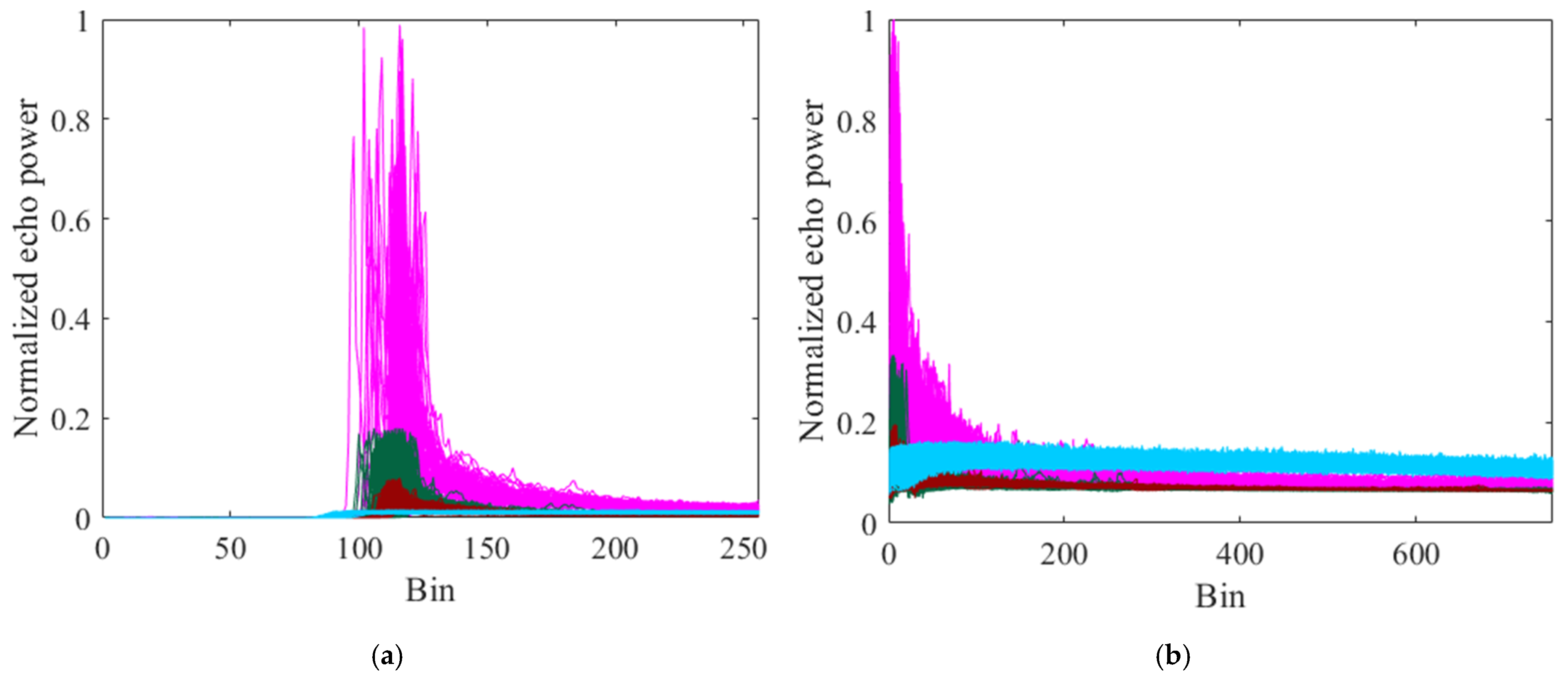
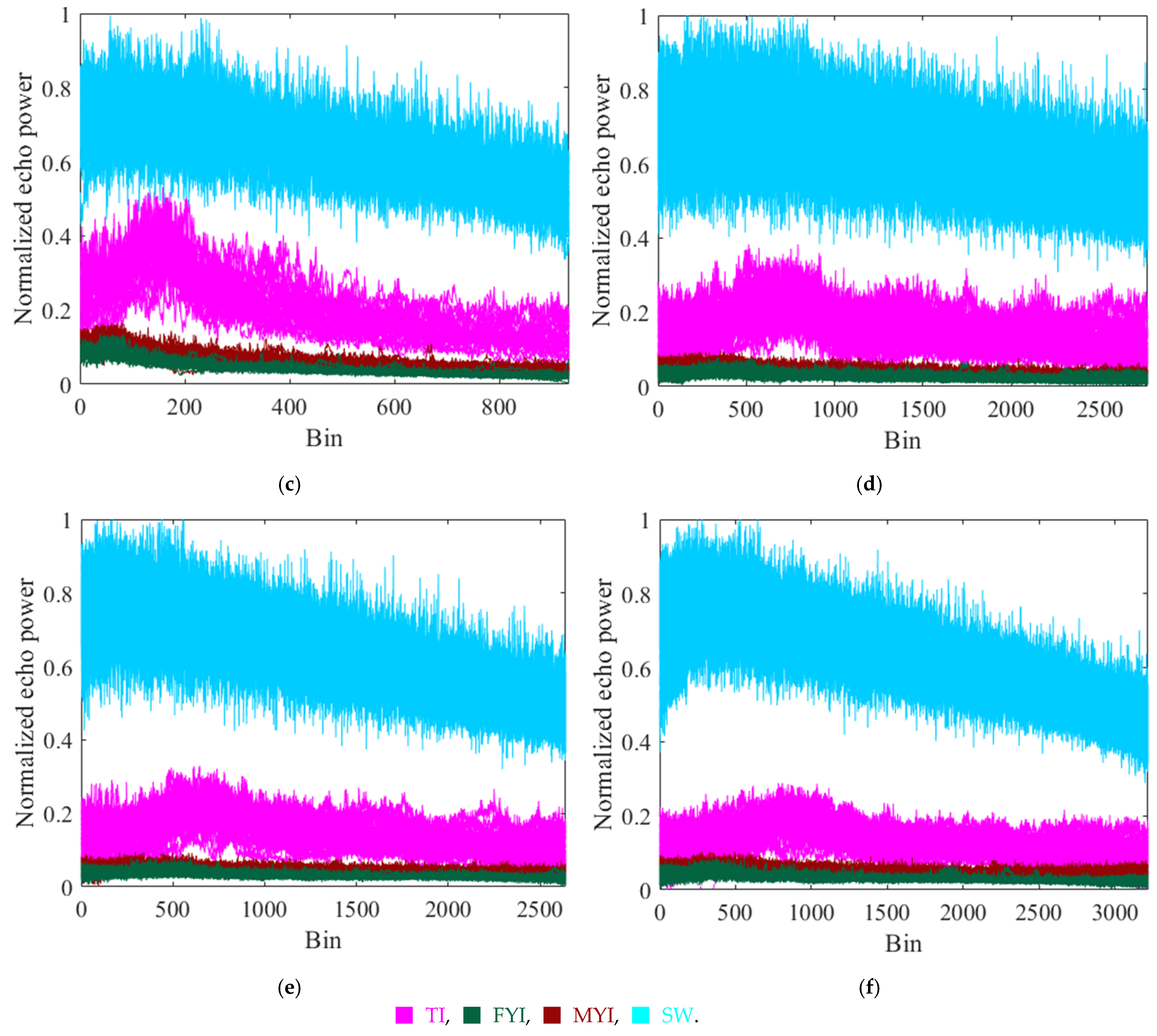
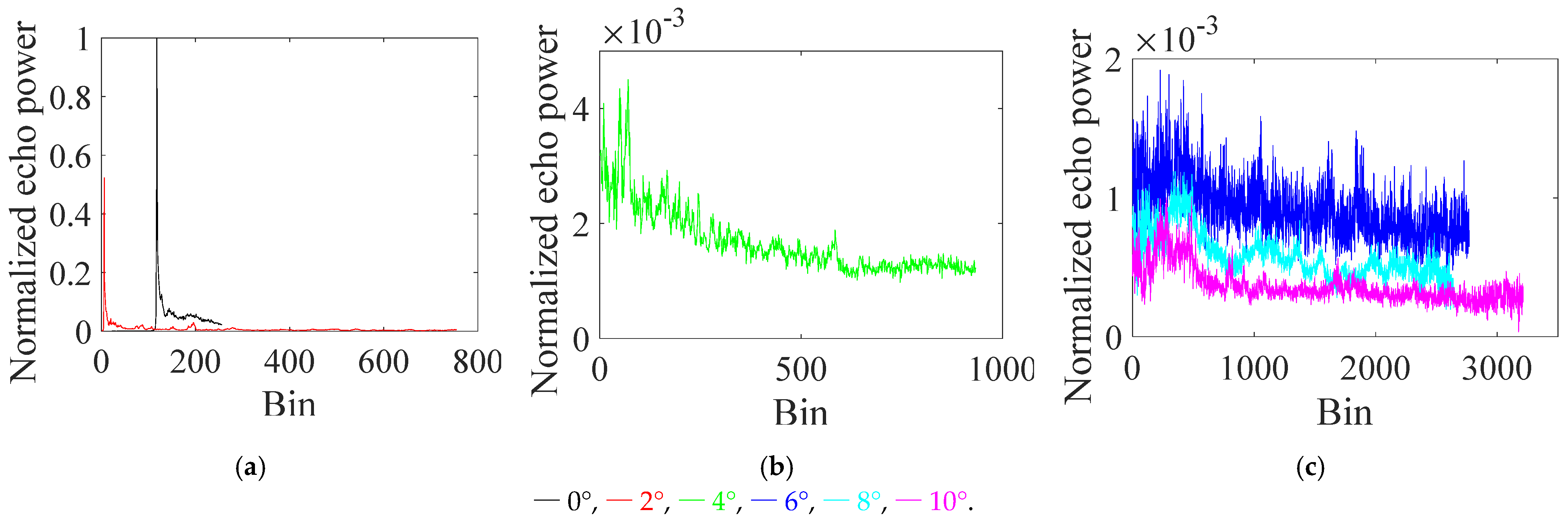
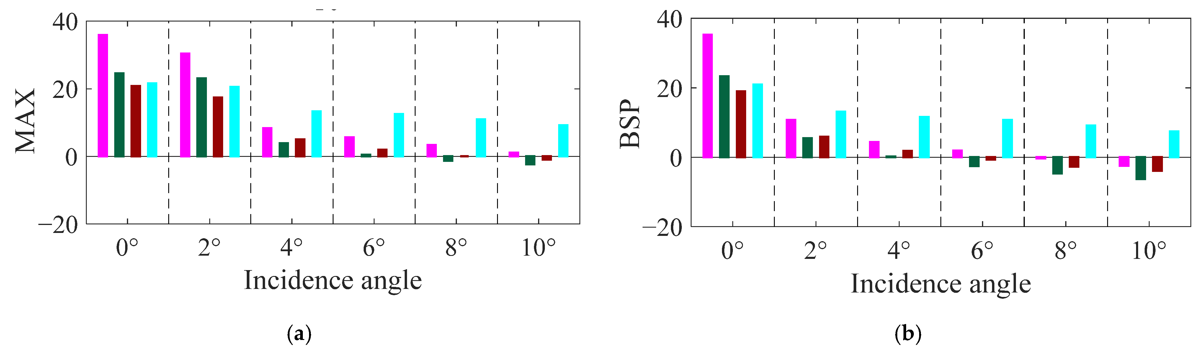
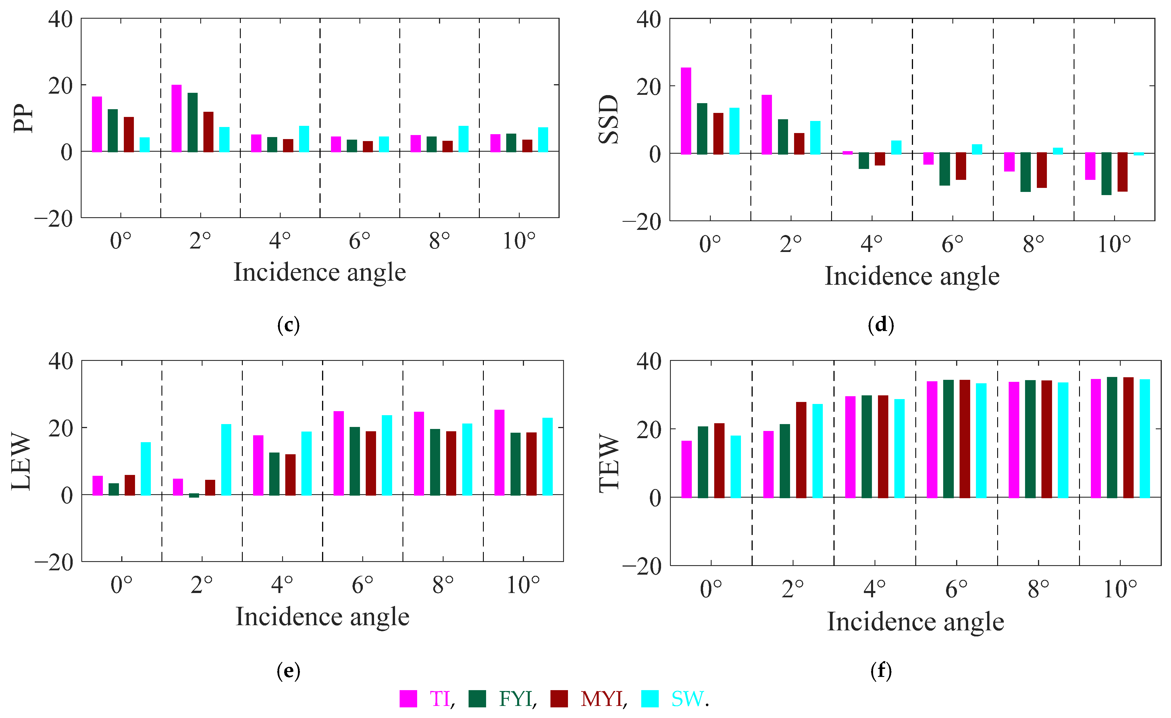
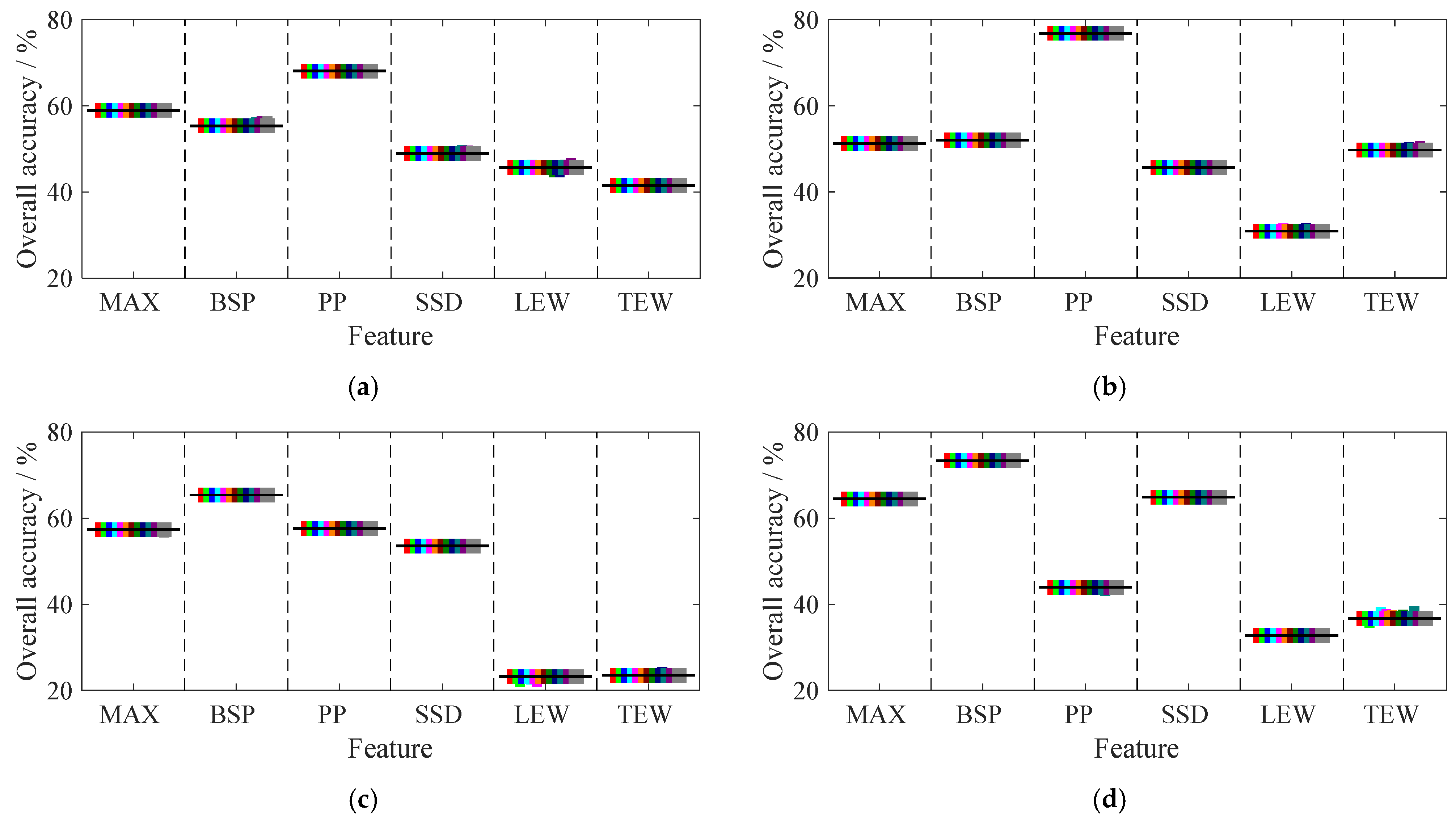
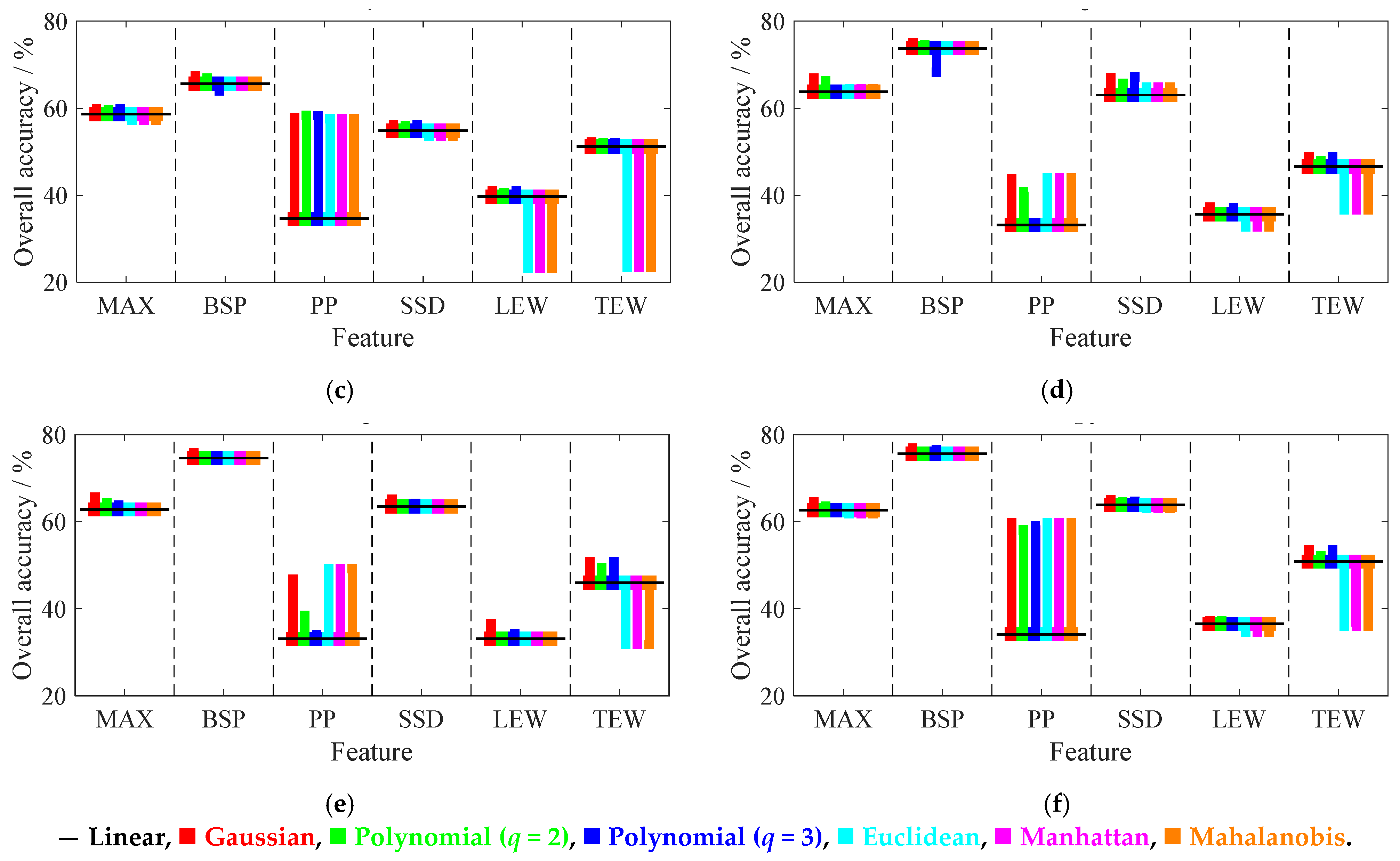
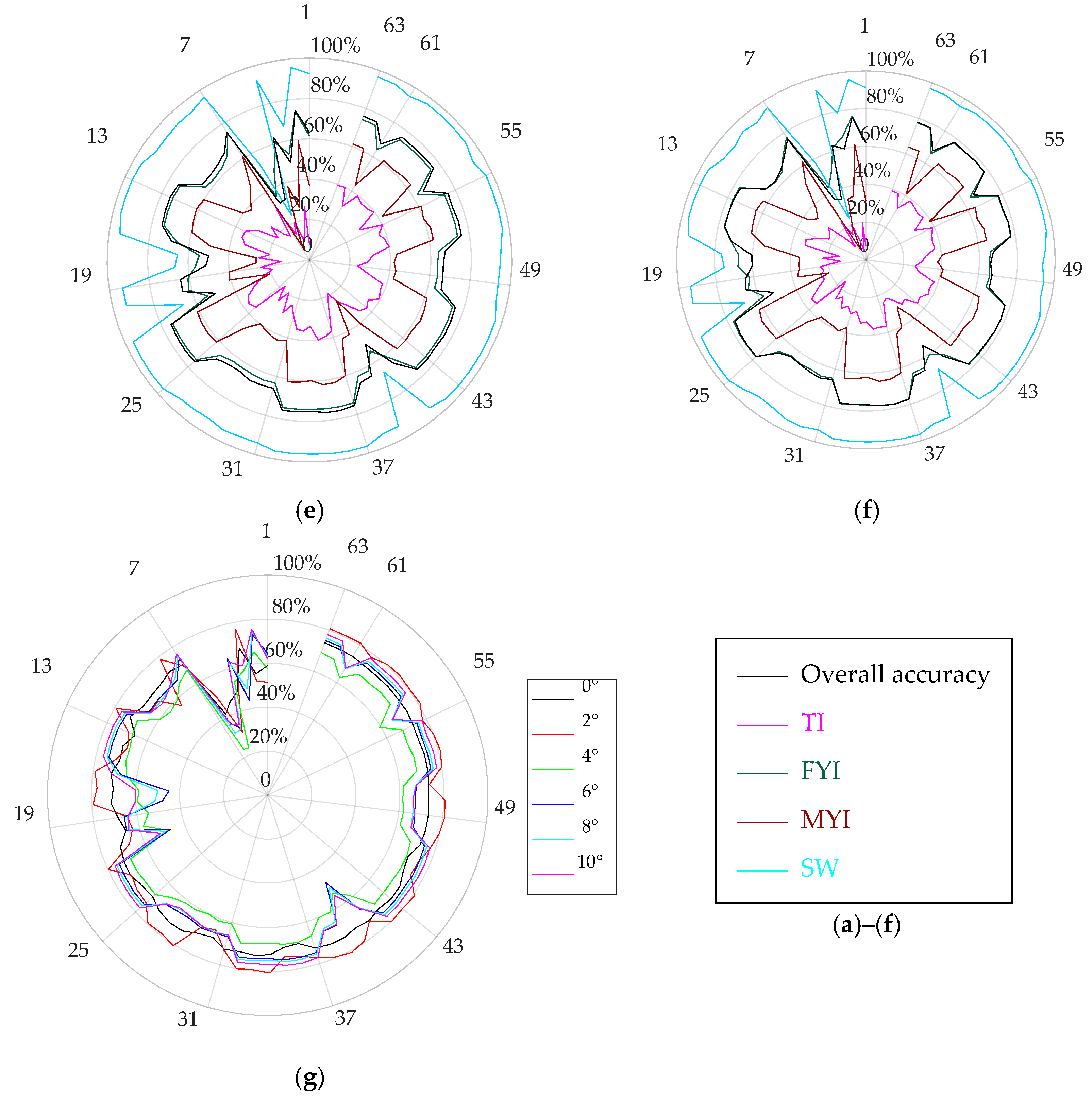
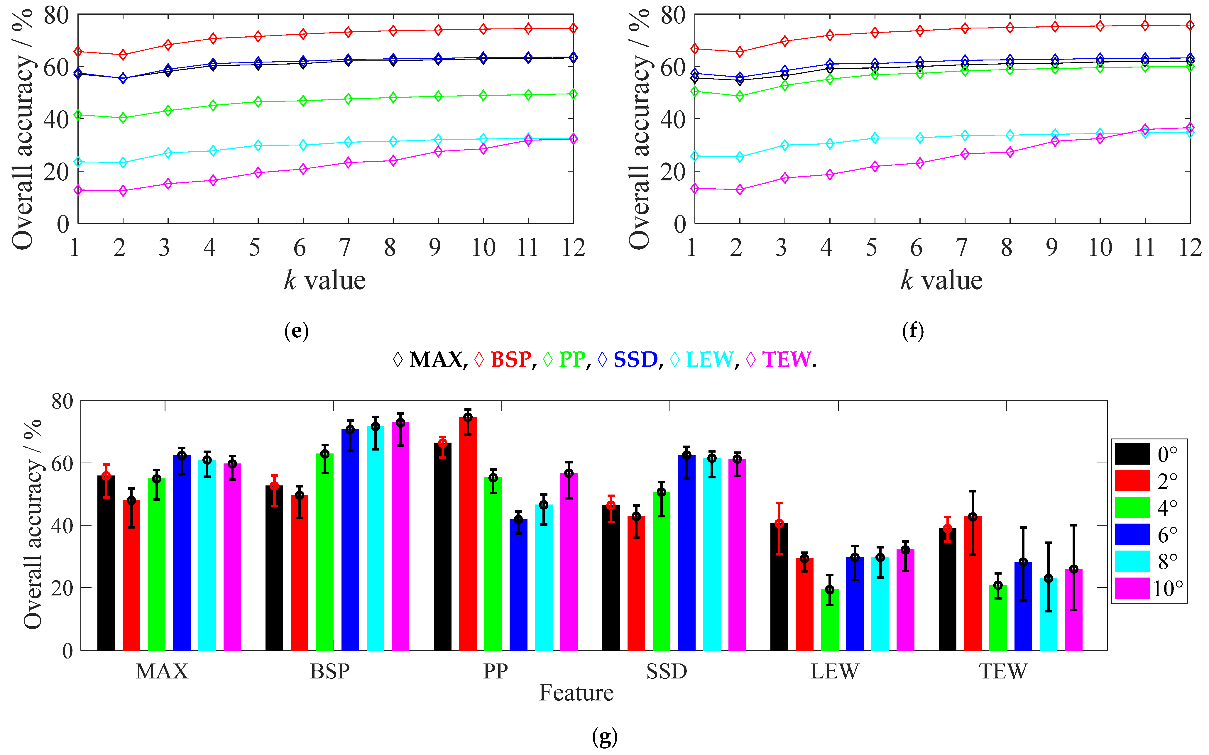
In this study, the sets of three incidence angles reveal their own characteristics in sea ice types and sea water recognition using single features of SWIM data. At 0–2°, PP, as a widely used feature, has higher accuracy in sea ice and sea water discrimination [14,46,51,52]; MAX is also a useful parameter in sea ice classification [13], and BSP, as a most popular parameter, can play an important role at six incidence angles [15,17,50]. At 6–10°, BSP is the best feature coincident with scatterometers and SARs [28,53], and MAX and SSD behave better and are also useful at 0–2° [15,16,17,
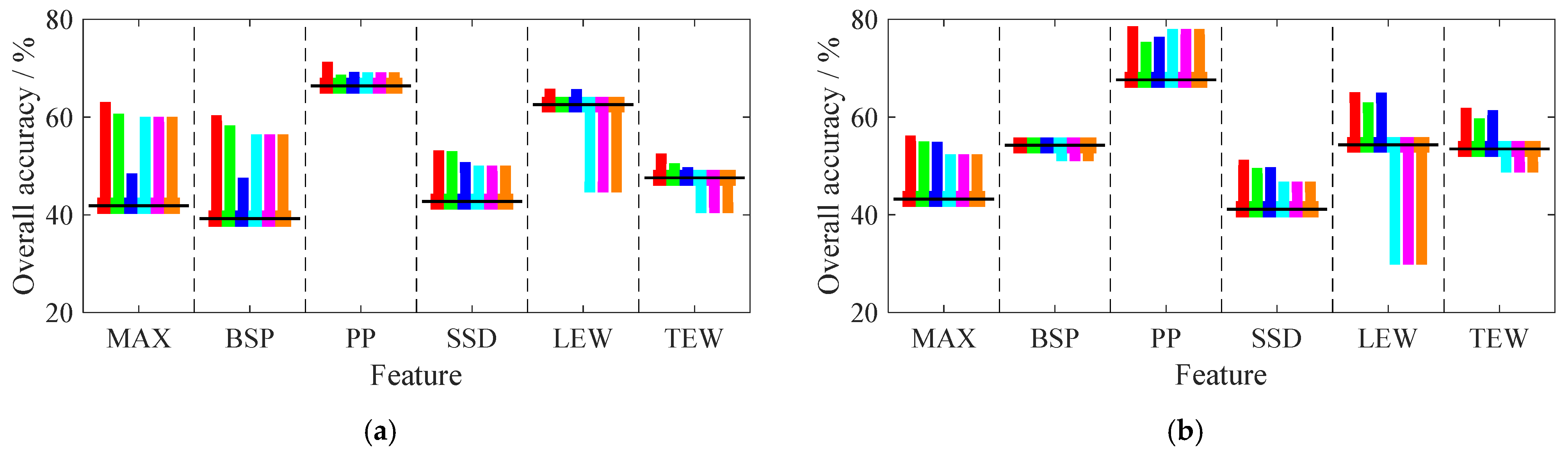
52]. At 4°, BSP, PP and MAX have better features in agreement with 0–2°; BSP has the highest accuracy consistent with 6–10° and it is indicated that 4° has properties of both 0–2° and 6–10°. In prior studies in multifeature combinations at 0°, the optimal combinations were BSP, MAX, PP and SSD [17], BSP, MAX, PP, LEW and TEW [16], MAX, PP, LEW, TEW and TES (trailing edge slope is MAX divided by TEW) [13], PP, SSD, LEW and LTPP (late tail to peak power ratio) [14], which is similar to our results (MAX, BSP, PP, SSD, LEW and TEW).
Zygmuntowska et al. [13] showed a classification performance of 78.7% (FYI, PP and TEW) and 81.7% (MYI, MAX and TEW) using the Bayesian method based on echo waveforms of the CryoSat-2 radar altimeter. Rinne and Similä [14] obtained classification accuracies of FYI (<70 cm) at 15–26%, FYI (>70 cm) at 75–92% and MYI at 77–92% in the Kara Sea in March 2014 using KNN based on Cryosat-2 data. Shen et al. [15] applied a random forest (RF) machine learning approach to obtain classification performances of 82.58% for FYI and 72.53% for MYI. Shu et al. [17] achieved an overall classification performance of 92.7 ± 3.3% (FYI) and 83.8 ± 3.59% (MYI) using the object-based RF (ORF) method based on Cryosat-2 data. These studies were validated by AARI sea ice charts. Aldenhoff et al. [52] introduced IMP (scaled inverse mean power) to improve the distinguishing FYI and MYI, which could enhance contrast when waveforms have similar peak values. The classification accuracies of thin ice and MYI are lower than those of other categories, and sea water has a higher classification performance, which agrees with our results. The classification accuracies of FYI and MYI are lower than those of Shen et al. [15] and Shu et al. [17], and new methods should be used for sea ice classification of SWIM data in future work.
Snow has an important influence on sea ice classification results, especially on MYI recognition. The Ku band can penetrate the snow layer to the snow-ice interface in theory, but wet snow makes the signal power dissipate and changes the characteristics of echo waveforms significantly, such as TEW [54]. MYI loads thicker snow than FYI. Thus, snow cover plays a more important role in MYI recognition of the Ku band [55]. It is necessary to study the effect of snow coverage on the microwave signal of sea ice types. Touzi [56] proposed a new scattering vector model for the expression of coherent target scattering based on polarimetric C-band SAR data, which could make coherent and partially coherent target scattering unified and decomposed. The symmetric scattering type phase in this model particularly exhibited a hopeful prospect for wetland classification, which would be useful for the study of snow coverage. Muhuri et al. [57] developed a mapping method of snow coverage using the Touzi eigenvalue-eigenvector-based decomposition parameters based on RADARSAT-2 C-band polarimetric SAR data. The results were comparable to those from spaceborne optical images, and agreed well with real-time field measurements. This research will represent the reference for the influence analysis of snow coverage on sea ice classification at small incidence angles. Moreover, this research will also be used for the ability comparison of the small, normal and medium-incidence sensors in sea ice classification.
Other wave features can be analyzed in sea ice classification, such as IMP and TES. Inverse mean power (IMP) [52] is calculated as follows:
IMP   = n θ i θ = 1 n θ P i θ · 2   ×   10 13 , unit :   W 1 ,  
IMP represents the total power contained in one waveform. This parameter is scaled by 2 × 10⁻¹³ to avoid too small values, and hence increases readability. The trailing edge slope (TES) is MAX divided by TEW and expresses the falling rate of the trailing edge of the waveform.
TES   = P max θ TEW , unit :   W .
The overall accuracies and F1 scores of IMP and TES at small incidence angles are shown in Table 10. TES behaves better than TEW and LEW, especially for 4°–10°, because TES combines the characteristics of MAX and TEW. IMP does not behave better than the above six features in overall accuracies, but performs well in the discrimination of FYI and MYI in the F1 scores.
In addition, because sea ice may ‘pollute’ SWIM wave products, SWIM data should include sea ice concentration information, which is the recognition of sea ice and sea water. In this study, sea water obtains a higher classification accuracy expressed by the F1 score compared with sea ice. At six incidence angles, the accuracies of every category are expressed by the F1 score, as shown in 
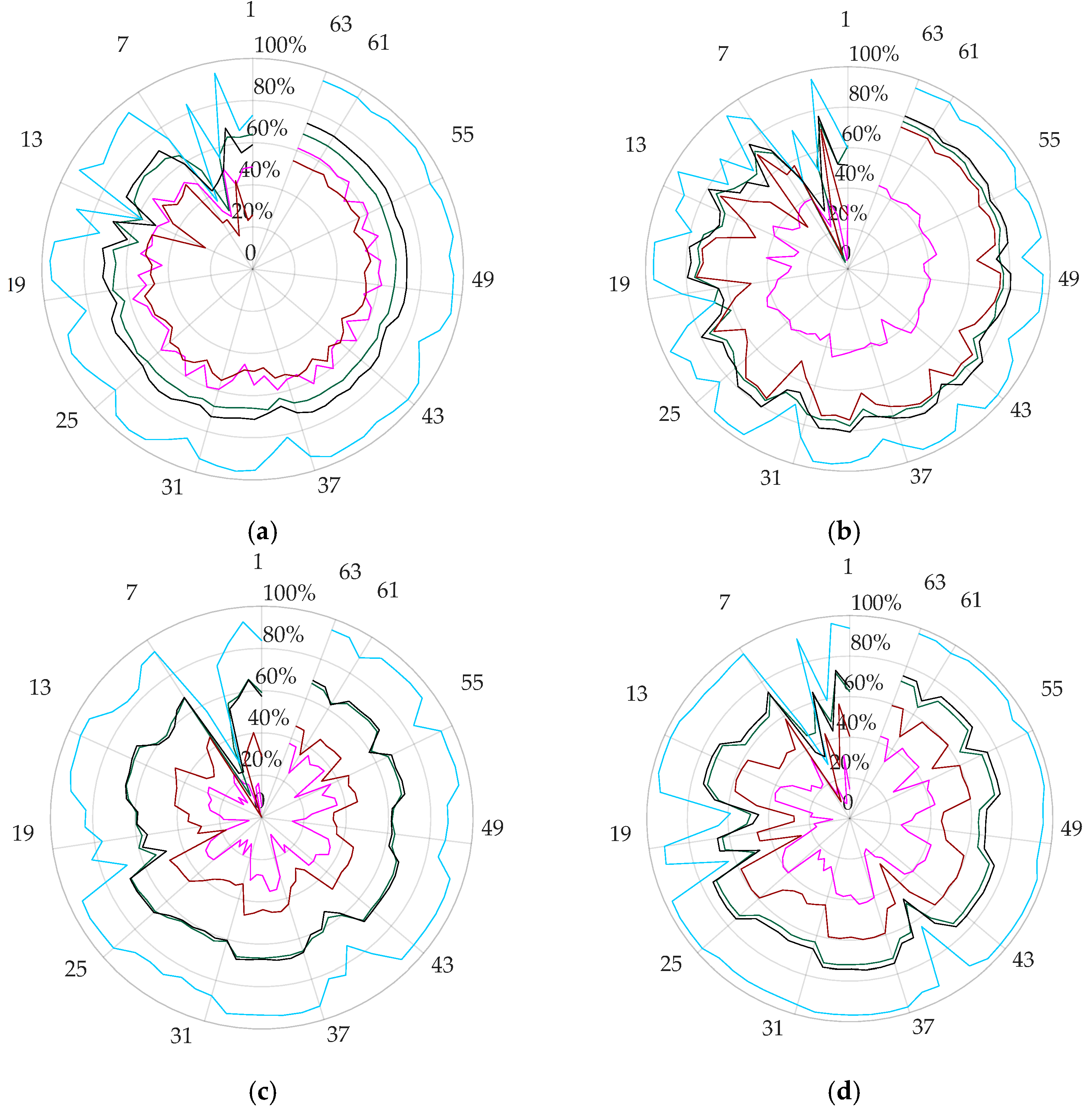
Table 11. The highest F1 scores of sea water at 0–2° and 6–10° are approximately 97%, and are slightly less than 95% at 4°. The highest overall accuracy is up to 97% at 6°, and the lowest is near 95% at 4°. For 0–2° and 6–10°, four out of the six top combinations are the same (No. 27, 43, 52, 57; and No. 55, 60, 62 63, respectively). In addition, 4° has the same multifeature combinations at both 0–2° and 6–10°, in agreement with the previous analysis in Section 3.1. Jiang et al. [46] distinguished sea ice and sea water using KNN and SVM based on wave features such as the PP of Haiyang-2 A/B, and their accuracies were approximately 80%. Müller et al. [58] monitored the Arctic seas using KNN and K-medoids based on wave features such as MAX of ENVISAT and SARAL with accuracies up to 94%. Thus, SWIM has strong abilities for sea ice and sea water recognition at multiple small incidence angles.

5. Conclusions

SWIM, as an innovative remote sensor and has the potential for sea ice classification. For the new detection mode using multiple small incidence angles of SWIM, our research focuses on the ability to discriminate sea ice types and sea water, classifier selection and setting, analysis of multifeature combinations, and application of the optimal multi-feature combination with the selected method.
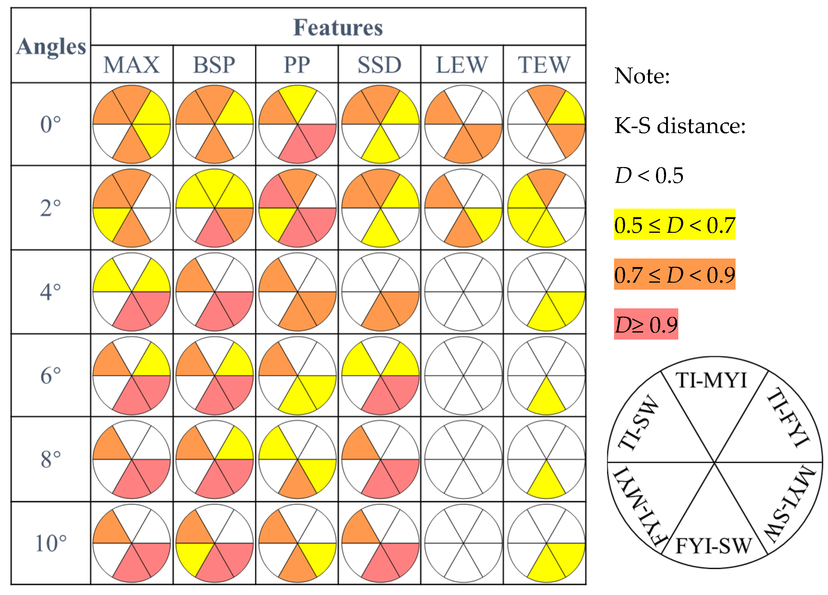
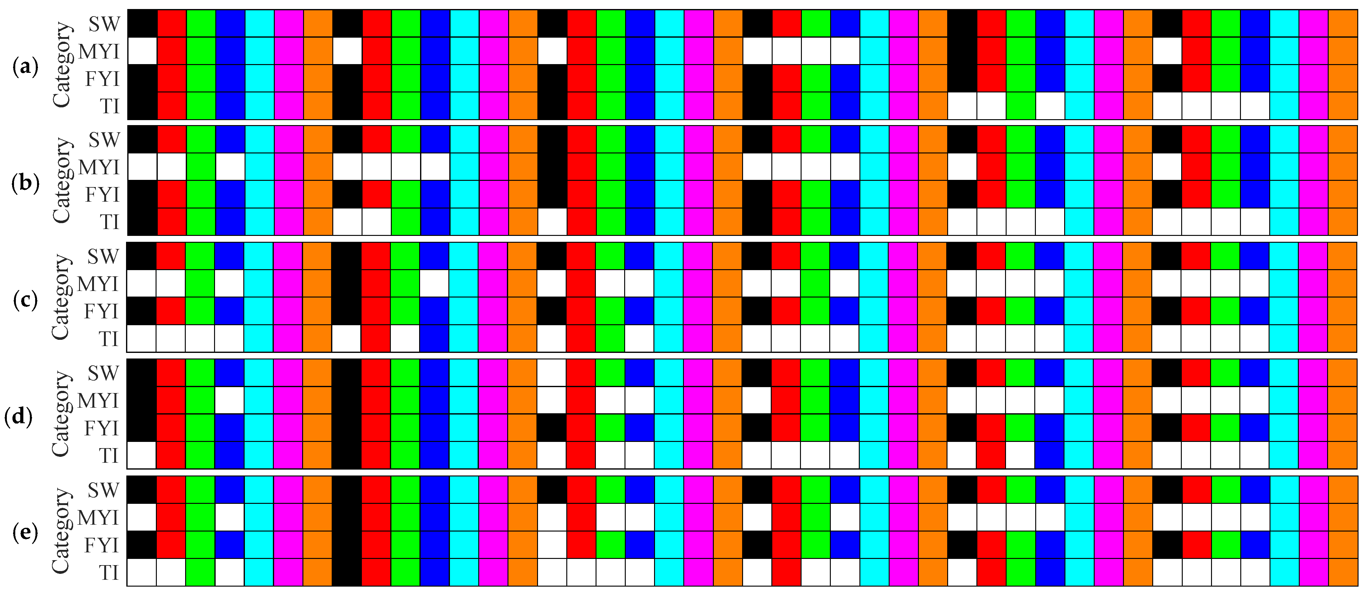
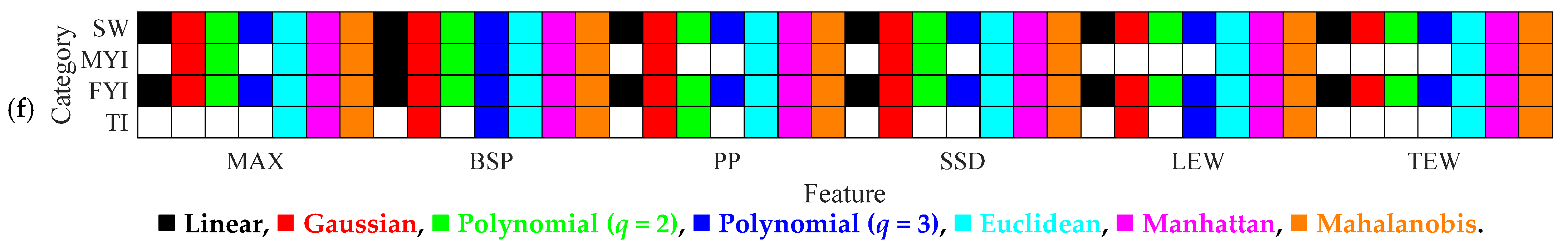
The SWIM data should be pretreated first. The waveforms of SWIM in the Arctic from October 2019 to April 2020 are given category labels of TI, FYI, MYI and SW using sea ice AARI charts. Then, waveform features are extracted, including the MAX, BSP, PP, SSD, LEW and TEW. The K-S distance is used to assess the ability to discriminate sea ice types and sea water. Moreover, KNN and SVM methods are introduced as sea ice classification methods.
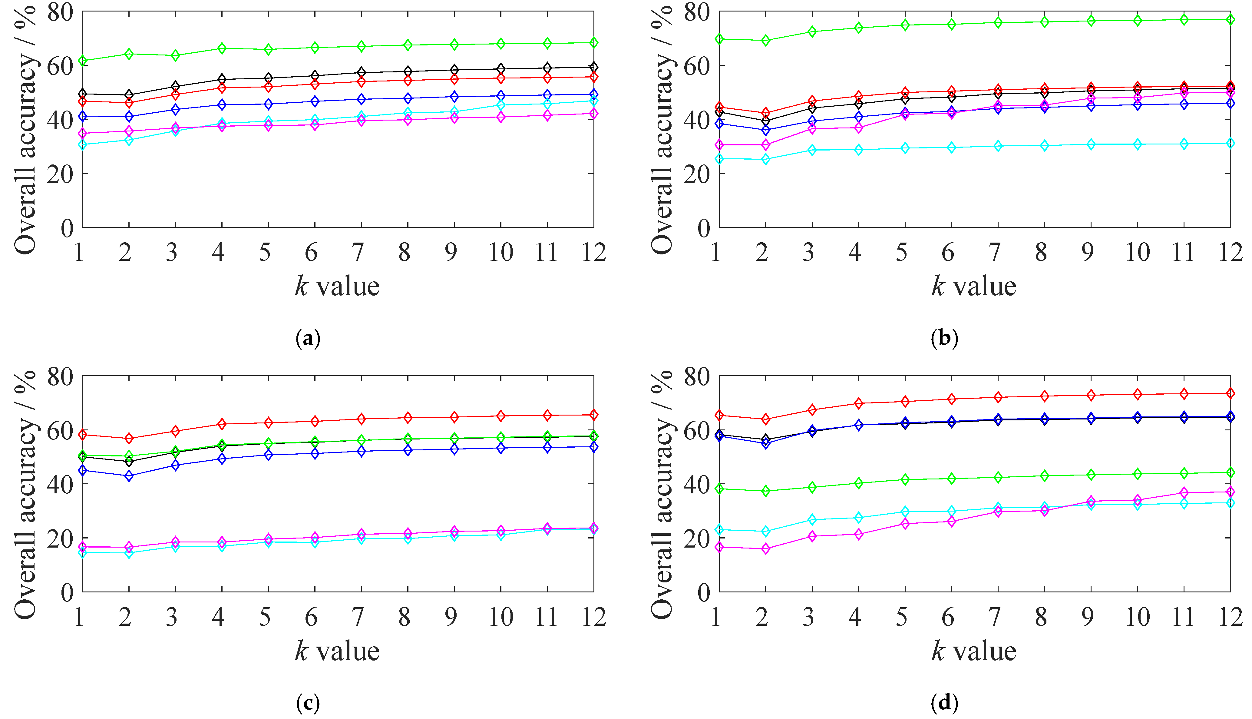
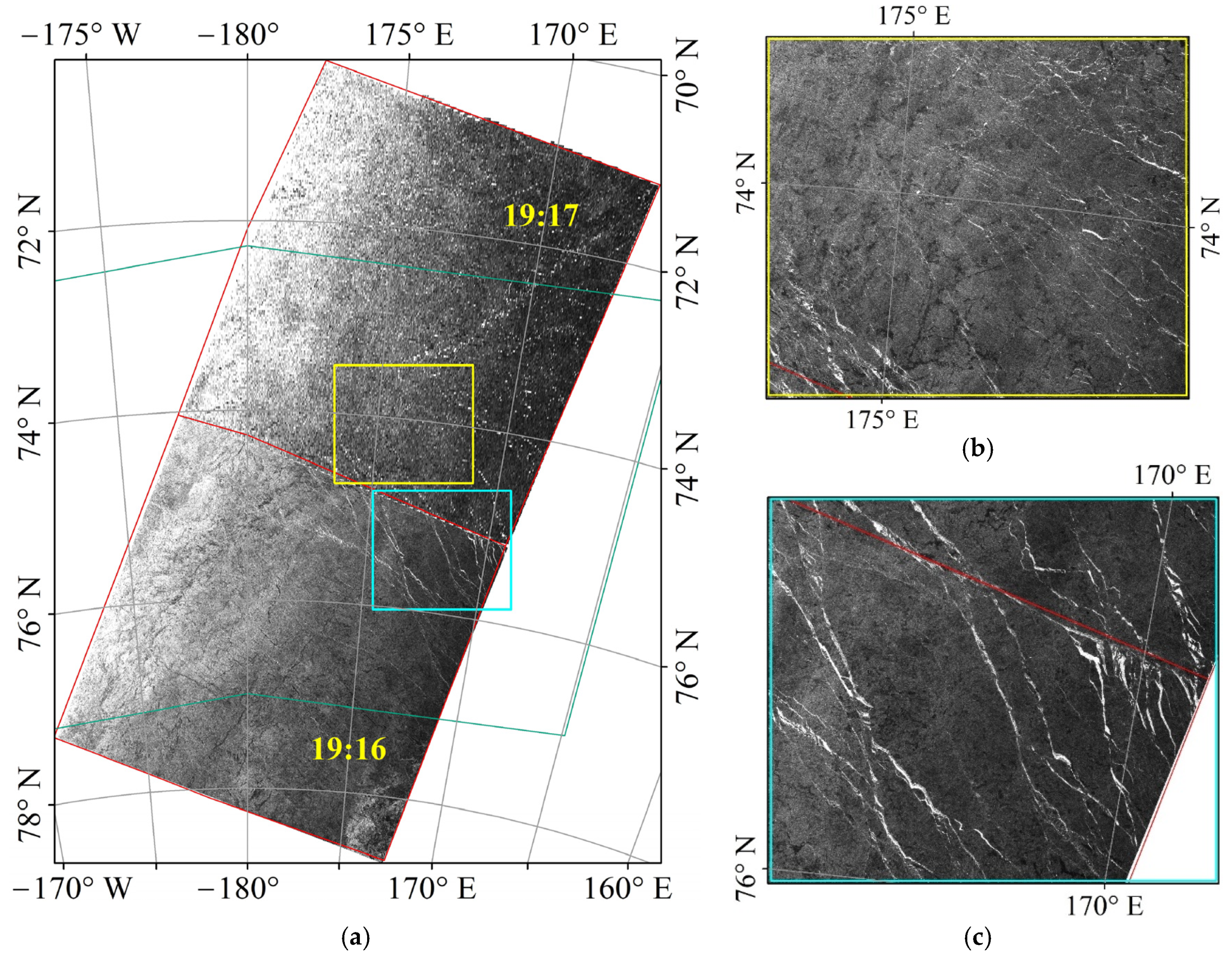
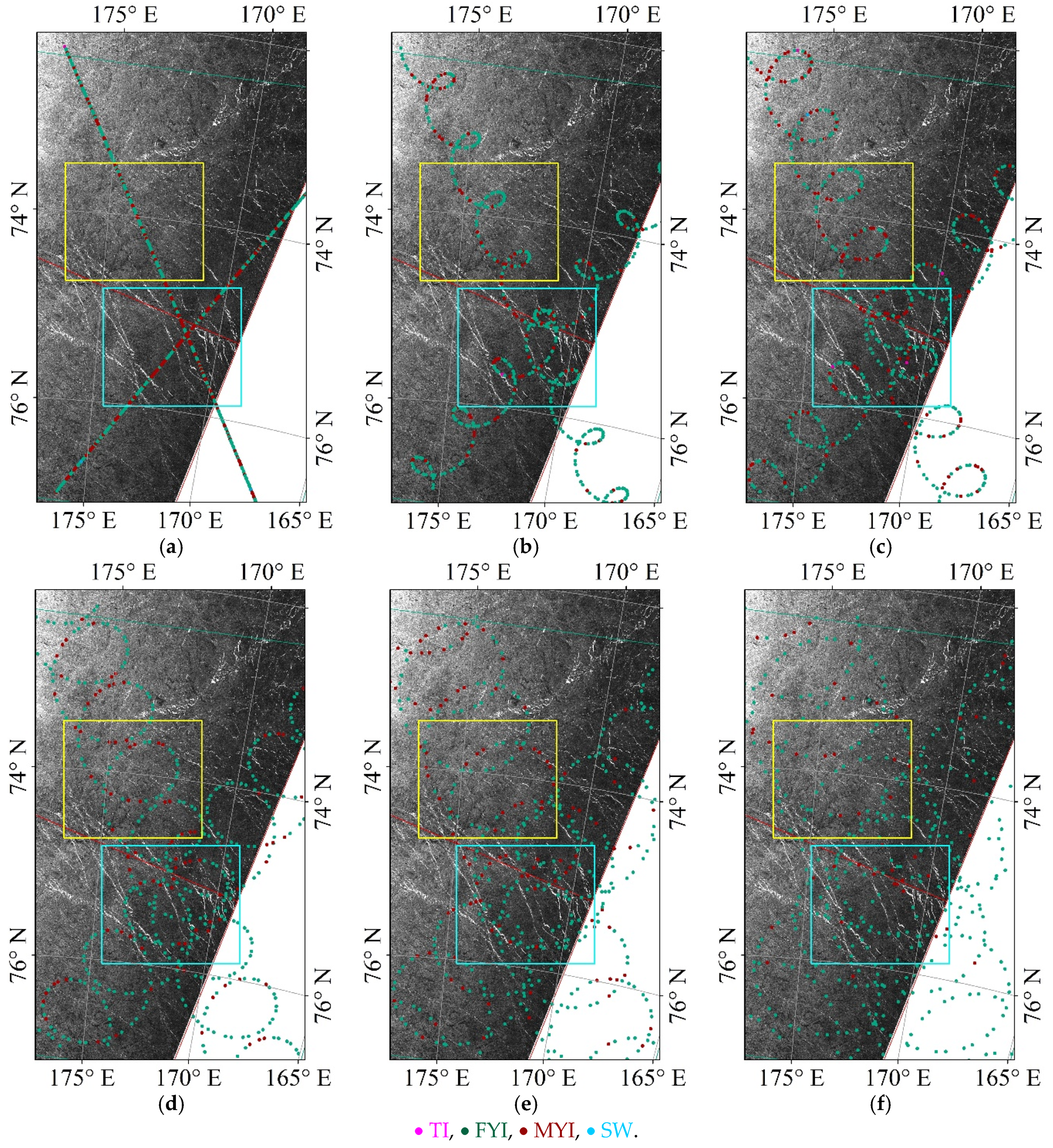
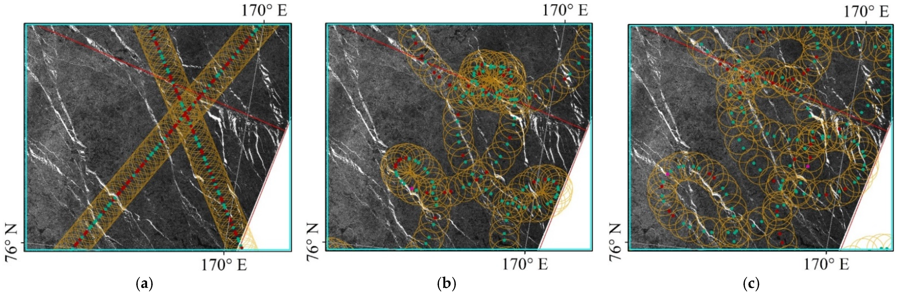
According to the waveform analysis combining the waveform features, the six incidence angles can be divided into three sets. At 0–2°, the waveform has a notable peak; at 6–10°, the waveform is flat; and 4° seems to be a transition between 0–2° and 6–10°. LEW and TEW have difficulty correctly discriminating because of fluctuations. The discrimination ability of single features using the K-S distance shows that the waveform features at all incidence angles distinguish between sea ice and sea water better than among sea ice types. MYI and TI are difficult to discriminate. LEW behaves the worst in distinguishing the categories at 4–10°. It is concluded that the three incidence sets have different discrimination abilities. These results agree with the waveform analysis. The overall accuracies of six waveform features for the SVM method using the Gaussian kernel at 0–10° are the highest, those for the linear kernel are the lowest, polynomial kernel 3 performs slightly better than polynomial kernel 2, and the three distances of the KNN method behave similarly. However, the SVM clearly misses the detection of sea ice types, especially MYI and TI. Therefore, the KNN method (the Euclidean distance and k equal to 11) is chosen to distinguish sea ice types and sea water. Sea ice classification results based on multifeature combinations at small incidence angles with the KNN method show that the highest overall accuracy is up to 81% at 2°, and the lowest is approximately 70% at 4°. The three incidence sets have differences, and 4° behaves similarly to 6–8°. The features of the PP and BSP have better discrimination abilities both in the analysis of the waveform and K-S distance and in multi-feature combinations. However, the SSD is not a better feature in the former analysis but plays a significant role in multifeature combinations. Moreover, LEW and TEW have difficulty recognizing sea ice types but are useful in multifeature combinations. The analysis of a single feature is different from the multifeature combination. Moreover, the top multifeature combinations with the KNN method are applied for randomly selected data in one day that are not filtered. The results suggested that optimal multifeature combinations with the KNN method are practical. Furthermore, the top multi-feature combinations with the KNN method are also applied for sea ice classification in the local regions, and the results are analyzed and compared with Sentinel-1 SAR images. The SWIM data are only filtered simply, so the classification results are representative and universally significant. It is concluded that optimal multifeature combinations with the KNN method are effective in sea ice classification.
Our results are compared with those of other studies and have better consistency. Moreover, sea water has very high classification accuracies of more than 96% at 0–2° and 6–10°, which meets the SWIM demand of sea ice discrimination. The influence of snow coverage is also discussed. Furthermore, the introduction of new waveform features can contribute to improving the classification accuracies, such as TES and IMP. Therefore, our results confirm the potential of sea ice recognition using the new data of SWIM. A sea ice classification method at small incidence angles is proposed, which can fill the gap in the research on sea ice monitoring of microwave remote sensing at small incident angles. Moreover, our work can also greatly promote new sea ice detection technology and application in the Arctic and Antarctic with significant theoretical and practical values.
In future work, more SWIM data of new ice years in the Arctic should be used to promote research on sea ice classification. The recognition abilities of new features and feature combinations, such as TES and IMP, will be evaluated further. Moreover, other classification methods, such as deep learning and SIR, will be assessed for their classification abilities, and the effect of snow coverage will also be considered. The abilities of the small, normal and medium-incidence sensors in sea ice classification will be investigated in depth.

Author Contributions

Conceptualization, M.L., J.Z., L.S. and X.Z.; data curation, M.L., and R.Y.; Methodology, M.L., J.W., and X.Z.; software, M.L.; Validation, M.L., Y.X., P.C. and X.Z.; writing—original draft, M.L.; Writing—review & editing, M.L., S.Z. and X.Z. All authors have read and agreed to the published version of the manuscript.

Funding

This research was funded in part by the National Natural Science Foundation of China under grant 41976173, 61971455, and 41976168; the Shandong Provincial Natural Science Foundation, China under grant ZR2019MD016; the Shandong joint fund of National Natural Science Foundation of China under grant U2006207; and the Ministry of Science and Technology of China and the European Space Agency through the Dragon-5 Program under grant 577889.

Institutional Review Board Statement

Not applicable.

Informed Consent Statement

Not applicable.

Data Availability Statement

The SWIM datasets can be found at https://www.aviso.altimetry.fr/en/home.html, accessed on 30 April 2020. Sentinel-1A/B SAR images are provided by https://asf.alaska.edu/, accessed on 30 April 2020. Sea ice charts of AARI are from http://www.aari.ru/, accessed on 30 April 2020.

Acknowledgments

Sea ice classification was based on the SWIM. Sea ice charts were provided by the AARI. The accuracy evaluation of sea ice classification was supported partly by Sentinel-1 SAR data.

Conflicts of Interest

The authors declare no conflict of interest.

Appendix A

The 63 multi-feature combinations are shown in Table A1.
Table A1. The 63 multi-feature combinations.
No.CombinationsNo.CombinationsNo.Combinations
1{MAX}22{MAX-BSP-PP}43{MAX-BSP-PP-LEW}
2{BSP}23{MAX-BSP-SSD}44{MAX-BSP-PP-TEW}
3{PP}24{MAX-BSP-LEW}45{MAX-BSP-SSD-LEW}
4{SSD}25{MAX-BSP-TEW}46{MAX-BSP-SSD-TEW}
5{LEW}26{MAX-PP-SSD}47{MAX-BSP-LEW-TEW}
6{TEW}27{MAX-PP-LEW}48{MAX-PP-SSD-LEW}
7{MAX-BSP}28{MAX-PP-TEW}49{MAX-PP-SSD-TEW}
8{MAX-PP}29{MAX-SSD-LEW}50{MAX-PP-LEW-TEW}
9{MAX-SSD}30{MAX-SSD-TEW}51{MAX-SSD-LEW-TEW}
10{MAX-LEW}31{MAX-LEW-TEW}52{BSP-PP-SSD-LEW}
11{MAX-TEW}32{BSP-PP-SSD}53{BSP-PP-SSD-TEW}
12{BSP-PP}33{BSP-PP-LEW}54{BSP-PP-LEW-TEW}
13{BSP-SSD}34{BSP-PP-TEW}55{BSP-SSD-LEW-TEW}
14{BSP-LEW}35{BSP-SSD-LEW}56{PP-SSD-LEW-TEW}
15{BSP-TEW}36{BSP-SSD-TEW}57{MAX-BSP-PP-SSD-LEW}
16{PP-SSD}37{BSP-LEW-TEW}58{MAX-BSP-PP-SSD-TEW}
17{PP-LEW}38{PP-SSD-LEW}59{MAX-BSP-PP-LEW-TEW}
18{PP-TEW}39{PP-SSD-TEW}60{MAX-BSP-SSD-LEW-TEW}
19{SSD-LEW}40{PP-LEW-TEW}61{MAX-PP-SSD-LEW-TEW}
20{SSD-TEW}41{SSD-LEW-TEW}62{BSP-PP-SSD-LEW-TEW}
21{LEW-TEW}42{MAX-BSP-PP-SSD}63{MAX-BSP-PP-SSD-LEW-TEW}

References

  1. Dierking, W.; Busche, T. Sea ice monitoring by L-band SAR: An assessment based on literature and comparisons of JERS-1 and ERS-1 imagery. IEEE Trans. Geosci. Remote Sens. 2006, 44, 957–970. [Google Scholar] [CrossRef]
  2. Stroeve, J.; Notz, D. Changing state of Arctic sea ice across all seasons. Environ. Res. Lett. 2018, 13, 103001. [Google Scholar] [CrossRef]
  3. SimilÄ, M.; Mäkynen, M.; Heiler, I. Comparison between C band synthetic aperture radar and 3-D laser scanner statistics for the Baltic Sea ice. J. Geophys. Res. Ocean. 2010, 115, C10056. [Google Scholar] [CrossRef]
  4. Swan, M.A.; Long, G.D. Multiyear Arctic Sea Ice Classification Using Quikscat. IEEE Trans. Geosci. Remote Sens. 2012, 50, 3317–3326. [Google Scholar] [CrossRef]
  5. Ezraty, R.; Cavanié, A. Intercomparison of backscatter maps over Arctic sea ice from NSCAT and the ERS scatterometer. J. Geophys. Res. Ocean. 1999, 104, 11471–11483. [Google Scholar] [CrossRef]
  6. Belchansky, G.I.; Douglas, D.C. Classification Methods for Monitoring Arctic Sea Ice Using OKEAN Passive/Active Two-Channel Microwave Data. Remote Sens. Environ. 2000, 73, 307–322. [Google Scholar] [CrossRef]
  7. Kwok, R. Annual cycles of multiyear sea ice coverage of the Arctic Ocean: 1999–2003. J. Geophys. Res. Ocean. 2004, 109, C11004. [Google Scholar] [CrossRef] [Green Version]
  8. Ochilov, S.; Clausi, D.A. Operational SAR sea-ice image classification. IEEE Trans. Geosci. Remote Sens. 2012, 50, 4397–4408. [Google Scholar] [CrossRef]
  9. Liu, M.; Dai, Y.; Zhang, J.; Ren, G.; Meng, J.; Zhang, X. The research on the object-based method of sea ice classification of high-resolution quad-polarization SAR data. Haiyang Xuebao 2013, 35, 80–87. (In Chinese) [Google Scholar] [CrossRef]
  10. Komarov, A.S.; Buehner, M. Automated detection of ice and open water from dual-polarization RADARSAT-2 images for data assimilation. IEEE Trans. Geosci. Remote Sens. 2017, 50, 1–15. [Google Scholar] [CrossRef]
  11. Tan, W.; Li, J.; Xu, L.; Chapman, M.A. Semiautomated Segmentation of Sentinel-1 SAR Imagery for Mapping Sea Ice in Labrador Coast. IEEE J. Sel. Top. Appl. Earth Obs. Remote Sens. 2018, 11, 1–14. [Google Scholar] [CrossRef]
  12. Drinkwater, M.R.; Carsey, F.D. Observations of the late-summer to fall sea ice transition with the 14.6 GHz Seasat scatterometer. IEEE 1991, 3, 1597–1600. [Google Scholar] [CrossRef]
  13. Zygmuntowska, M.; Khvorostovsky, K.; Helm, V.; Sandven, S. Waveform classification of airborne synthetic aperture radar altimeter over Arctic sea ice. Cryosphere 2013, 7, 1315–1324. [Google Scholar] [CrossRef] [Green Version]
  14. Rinne, E.; Similä, M. Utilisation of CryoSat-2 SAR altimeter in operational ice charting. Cryosphere 2016, 10, 121–131. [Google Scholar] [CrossRef] [Green Version]
  15. Shen, X.Y.; Zhang, J.; Meng, J.M.; Ke, C.Q. Sea ice type classification based on random forest machine learning with CryoSat-2 altimeter data. In Proceedings of the 2017 International Workshop on Remote Sensing with Intelligent Processing (RSIP), Shanghai, China, 18–21 May 2017; IEEE: Piscataway, NJ, USA, 2017. [Google Scholar] [CrossRef]
  16. Shen, X.; Jie, Z.; Xi, Z.; Meng, J.; Ke, C. Sea ice classification using CryoSat-2 altimeter data by optimal classifier-feature assembly. IEEE Geosci. Remote Sens. Lett. 2017, 14, 1948–1952. [Google Scholar] [CrossRef]
  17. Shu, S.; Zhou, X.; Shen, X.; Liu, Z.; Li, J. Discrimination of different sea ice types from CryoSat-2 satellite data using an Object-based Random Forest (ORF). Mar. Geod. 2019, 5, 1–21. [Google Scholar] [CrossRef]
  18. Cavanie, A.; Gohin, F.; Quilfen, Y. Identification of sea ice zones using the AMI-wind: Physical bases and applications to the FDP and CERSAT processing chains. Eur. Space Agency-Publ.-ESA SP 1994, 361, 1009. [Google Scholar]
  19. Gohin, F.; Cavanie, A. A first try at identification of sea ice using the three beam scatterometer of ERS-1. Int. J. Remote Sens. 1994, 15, 1221–1228. [Google Scholar] [CrossRef]
  20. Remund, Q.P.; Long, D.G. Sea-ice extent mapping using Ku-band scatterometer data. J. Geophys. Res. Ocean. 1999, 104, 11515–11527. [Google Scholar] [CrossRef] [Green Version]
  21. Oza, S.R.; Singh, R.; Vyas, N.K.; Gohil, B.S.; Sarkar, A. Spatio-Temporal Coherence Based Technique for Near-Real Time Sea-Ice Identification from Scatterometer Data. J. Indian Soc. Remote Sens. 2011, 39, 147–152. [Google Scholar] [CrossRef]
  22. Breivik, L.A.; Eastwood, S.; Lavergne, T. Use of C-Band Scatterometer for Sea Ice Edge Identification. IEEE Trans. Geosci. Remote Sens. 2012, 50, 2669–2677. [Google Scholar] [CrossRef]
  23. Rivas, M.B.; Verspeek, J.; Verhoef, A.; Stoffelen, A. Bayesian Sea Ice Detection with the Advanced Scatterometer ASCAT. IEEE Trans. Geosci. Remote Sens. 2012, 50, 2649–2657. [Google Scholar] [CrossRef]
  24. Remund, Q.P.; Long, D.G. A Decade of QuikSCAT Scatterometer Sea Ice Extent Data. IEEE Trans. Geosci. Remote Sens. 2014, 52, 4281–4290. [Google Scholar] [CrossRef] [Green Version]
  25. Zou, J.; Tao, Z.; Guo, M.; Cui, S. The study on an Antarctic sea ice identification algorithm of the HY-2A microwave scatterometer data. Acta Oceanol. Sin. 2016, 35, 74–79. [Google Scholar] [CrossRef]
  26. Bi, H.; Zhang, J.; Wang, Y.; Zhang, Z.; Zhang, Y.; Fu, M.; Huang, H.; Xu, X. Arctic Sea Ice Volume Changes in Terms of Age as Revealed from Satellite Observations. IEEE J. Sel. Top. Appl. Earth Obs. Remote Sens. 2018, 11, 1–15. [Google Scholar] [CrossRef]
  27. Rivas, M.B.; Stoffelen, A. New Bayesian Algorithm for Sea Ice Detection with QuikSCAT. IEEE Trans. Geosci. Remote Sens. 2011, 49, 1894–1901. [Google Scholar] [CrossRef]
  28. Otosaka, I.; Rivas, M.B.; Stoffelen, A. Bayesian Sea Ice Detection with the ERS Scatterometer and Sea Ice Backscatter Model at C-Band. IEEE Trans. Geosci. Remote Sens. 2017, 56, 2248–2254. [Google Scholar] [CrossRef]
  29. Long, D.G.; Early, D.S.; Drinkwater, M.R. Enhanced resolution ERS-1 scatterometer imaging of Southern Hemisphere polar ice. IEEE Int. Geosci. Remote Sens. Symp. 1994, 1, 156–158. [Google Scholar] [CrossRef]
  30. Meier, W.N.; Stroeve, J. Comparison of sea-ice extent and ice-edge location estimates from passive microwave and enhanced-resolution scatterometer data. Ann. Glaciol. 2008, 48, 65–70. [Google Scholar] [CrossRef] [Green Version]
  31. Wang, L.; Ding, Z.; Zhang, L.; Yan, C. Cfosat-1 realizes first joint observation of sea wind and waves. Aerosp. China 2019, 20, 22–29. [Google Scholar] [CrossRef]
  32. Xu, Y.; Liu, J.; Xie, L.; Sun, C.; Xian, D. China-France Oceanography Satellite (CFOSAT) simultaneously observes the typhoon-induced wind and wave fields. Acta Oceanol. Sin. 2019, 38, 158–161. [Google Scholar] [CrossRef]
  33. Hauser, D.; Tison, C.; Amiot, T.; Delaye, L.; Mouche, A.; Guitton, G.; Aouf, L.; Castillan, P. CFOSAT: A new Chinese-French satellite for joint observations of ocean wind vector and directional spectra of ocean waves. Remote Sens. Ocean. Inland Waters Tech. Appl. Chall. 2016, 9878T, 1–20. [Google Scholar] [CrossRef] [Green Version]
  34. Hauser, D.; Tison, C.; Amiot, T.; Delaye, L.; Corcoral, N.; Castillan, P. Swim: The first spaceborne wave scatterometer. IEEE Trans. Geosci. Remote Sens. 2017, 55, 3000–3014. [Google Scholar] [CrossRef] [Green Version]
  35. Hauser, D.; Tourain, C.; Hermozo, L.; Alraddawi, D.; Tran, N.T. New observations from the swim radar on-board cfosat: Instrument validation and ocean wave measurement assessment. IEEE Trans. Geosci. Remote Sens. 2020, 59, 5–26. [Google Scholar] [CrossRef]
  36. Lin, W.; Dong, X.; Portabella, M.; Lang, S.; He, Y.; Yun, R.; Wang, Z.; Xu, X.; Zhu, D.; Liu, J. A Perspective on the Performance of the CFOSAT Rotating Fan-Beam Scatterometer. IEEE Trans. Geosci. Remote Sens. 2019, 57, 627–639. [Google Scholar] [CrossRef] [Green Version]
  37. Nagler, T.; Rott, H.; Hetzenecker, M.; Wuite, J.; Potin, P. The sentinel-1 mission: New opportunities for ice sheet observations. Remote Sens. 2015, 7, 9371. [Google Scholar] [CrossRef] [Green Version]
  38. Arctic and Antaractic Research Institute (AARI). Available online: http://www.aari.ru/ (accessed on 30 April 2020).
  39. Zakharova, E.A.; Fleury, S.; Guerreiro, K.; Willmes, S.; Rémy, F.; Kouraev, A.V.; Heinemann, G. Sea Ice Leads Detection Using SARAL/AltiKa Altimeter. Mar. Geod. 2015, 38, 522–533. [Google Scholar] [CrossRef]
  40. Gommenginger, C.; Thibaut, P.; Fenoglio-Marc, L.; Quartly, G.; Deng, X.; Gómez-Enri, J.; Gao, Y. Retracking altimeter waveforms near the coasts. In Coastal Altimetry; Springer: Berlin/Heidelberg, Germany, 2011; pp. 61–101. [Google Scholar] [CrossRef]
  41. Laxon, S.W.; Giles, K.A.; Ridout, A.L.; Wingham, D.J.; Willatt, R.; Cullen, R.; Kwok, R.; Schweiger, A.; Zhang, J.; Haas, C.; et al. CryoSat-2 estimates of Arctic sea ice thickness and volume. Geophys. Res. Lett. 2013, 40, 732–737. [Google Scholar] [CrossRef] [Green Version]
  42. Wingham, D.J.; Francis, C.R.; Baker, S.; Bouzinac, C.; Brockley, D.; Cullen, R.; de Chateau-Thierry, P.; Laxon, S.; Mallow, U.; Mavrocordatos, C.; et al. CryoSat: A mission to determine the fluctuations in Earth’s land and marine ice fields. Adv. Space Res. 2006, 37, 841–871. [Google Scholar] [CrossRef]
  43. Zhang, X.; Zhu, Y.; Zhang, J.; Wang, Q.; Shi, L.; Meng, J.; Bao, M. Assessment of Arctic Sea Ice Classification Ability of Chinese HY-2B Dual-Band Radar Altimeter During Winter to Early Spring Conditions. IEEE J. Sel. Top. Appl. Earth Obs. Remote Sens. 2021, 14, 9855–9872. [Google Scholar] [CrossRef]
  44. Zhang, Z.; Yu, Y.; Shokr, M.; Li, X.; Ye, Y.; Cheng, X.; Hui, F. Intercomparison of Arctic Sea Ice Backscatter and Ice Type Classification Using Ku-Band and C-Band Scatterometers. IEEE Trans. Geosci. Remote Sens. 2021, 1–18. [Google Scholar] [CrossRef]
  45. Dabboor, M.; Montpetit, B.; Howell, S. Assessment of the High Resolution SAR Mode of the RADARSAT Constellation Mission for First Year Ice and Multiyear Ice Characterization. Remote Sens. 2018, 10, 594. [Google Scholar] [CrossRef] [Green Version]
  46. Jiang, C.; Lin, M.; Wei, H. A Study of the Technology Used to Distinguish Sea Ice and Seawater on the Haiyang-2A/B (HY-2A/B) Altimeter Data. Remote Sens. 2019, 11, 1490. [Google Scholar] [CrossRef] [Green Version]
  47. Liu, H.; Guo, H.; Zhang, L. Svm-based sea ice classification using textural features and concentration from radarsat-2 dual-pol scansar data. IEEE J. Sel. Top. Appl. Earth Obs. Remote Sens. 2015, 8, 1601–1613. [Google Scholar] [CrossRef]
  48. Hauser, D.; Caudal, G.; Rijckenberg, G.J.; Vidal-Madjar, D.; Laurent, G.; Lancelin, P. RESSAC: A new airborne FM/CW radar ocean wave spectrometer. IEEE Trans. Geosci. Remote Sens. 1992, 30, 981–995. [Google Scholar] [CrossRef]
  49. Ulaby, F.T.; Moore, R.K.; Fung, A.K. Microwave Remote Sensing: Active and Passive; Artech House Publishers: Fitchburg, MA, USA, 1986; Volume 2. [Google Scholar]
  50. Fredensborg Hansen, R.M.; Rinne, E.; Skourup, H. Classification of Sea Ice Types in the Arctic by Radar Echoes from SARAL/AltiKa. Remote Sens. 2021, 13, 3183. [Google Scholar] [CrossRef]
  51. Paul, S.; Hendricks, S.; Ricker, R.; Kern, S.; Rinne, E. Empirical parametri-zation of Envisat freeboard retrieval of arctic and Antarctic sea ice based on CryoSat-2: Progress in the ESA climate change initiative. Cryosphere 2018, 12, 2437–2460. [Google Scholar] [CrossRef] [Green Version]
  52. Aldenhoff, W.; Heuzé, C.; Eriksson, L.E.B. Sensitivity of Radar Altimeter Waveform to Changes in Sea Ice Type at Resolution of Synthetic Aperture Radar. Remote Sens. 2019, 11, 2602. [Google Scholar] [CrossRef] [Green Version]
  53. Zhang, Z.; Yu, Y.; Li, X.; Hui, F.; Cheng, X.; Chen, Z. Arctic sea ice classification using microwave scatterometer and radiometer data during 2002–2017. IEEE Trans. Geosci. Remote Sens. 2019, 57, 1–10. [Google Scholar] [CrossRef]
  54. Blanchard-Wrigglesworth, E.; Farrell, S.L.; Newman, T.; Bitz, C.M. Snow cover on Arctic sea ice in observations and an Earth System Model. Geophys. Res. Lett. 2015, 42, 10–342. [Google Scholar] [CrossRef] [Green Version]
  55. Guerreiro, K.; Fleury, S.; Zakharova, E.; Rémy, F.; Kouraev, A. Potential for estimation of snow depth on Arctic sea ice from CryoSat-2 and SARAL/AltiKa missions. Remote Sens. Environ. 2016, 186, 339–349. [Google Scholar] [CrossRef]
  56. Touzi, R. Target Scattering Decomposition in Terms of Roll-Invariant Target Parameters. IEEE Trans. Geosci. Remote Sens. 2006, 45, 73–84. [Google Scholar] [CrossRef]
  57. Muhuri, A.; Manickam, S.; Bhattacharya, A. Scattering Mechanism Based Snow Cover Mapping Using RADARSAT-2 C-Band Polarimetric SAR Data. IEEE J. Sel. Top. Appl. Earth Obs. Remote Sens. 2017, 10, 3213–3224. [Google Scholar] [CrossRef]
  58. Müller, F.L.; Dettmering, D.; Bosch, W.; Seitz, F. Monitoring the Arctic Seas: How Satellite Altimetry Can Be Used to Detect Open Water in Sea-Ice Regions. Remote Sens. 2017, 9, 551. [Google Scholar] [CrossRef] [Green Version]
Figure 1. SWIM beam rotation with incidence angles. (a) Schematic of the illumination geometry formed by the six beams during three macrocycles. One macrocycle comprises the illumination patterns formed by the six successively transmitted beams; these are not continuous in azimuth. (b) SWIM footprint distribution in the Arctic on 15 April 2020. (c) Schematic, using geographical coordinates, of a portion of the Earth’s surface sampled during approximately several macrocycles. Antenna aperture: 2° × 2°.
Remotesensing 14 00091 g001
Figure 2. Examples of normalized SWIM waveforms of sea water and sea ice types at six incidence angles: (a) 0°; (b) 2°; (c) 4°; (d) 6°; (e) 8°; (f) 10°.
Remotesensing 14 00091 g002aRemotesensing 14 00091 g002b
Figure 3. Echo waveforms of FYI at the six small incidence angles: (a) 0°–2°; (b) 4°; (c) 6°–10°.
Remotesensing 14 00091 g003
Figure 4. A waveform including negative echo powers (1 October 2019).
Remotesensing 14 00091 g004
Figure 5. Schematic of the sea surface using a two-scale model. The black curve expresses the long wave, while the blue curves show the short waves propagating on the long wave. The red lines represent the wave facets and the red arrows give denote normal direction, which illustrates the changes of local incidence angles.
Remotesensing 14 00091 g005
Figure 6. Values of every feature processed logarithmically and enlarged 10 times. (a) MAX; (b) BSP; (c) PP; (d) SSD; (e) LEW; (f) TEW.
Remotesensing 14 00091 g006aRemotesensing 14 00091 g006b
Figure 7. K-S distances between sea ice types and sea water using single features at small incidence angles.
Remotesensing 14 00091 g007
Figure 8. Overall accuracies of 13 groups of training data expressed by G1–G13 at six incidence angles: (a) 0°; (b) 2°; (c) 4°; (d) 6°; (e) 8°; (f) 10°.
Remotesensing 14 00091 g008aRemotesensing 14 00091 g008b
Figure 9. (af) Overall accuracies of six waveform features for different k values at small incidence angles: (a) 0°; (b) 2°; (c) 4°; (d) 6°; (e) 8°; (f) 10°. (g) Mean values of the overall accuracies are expressed by the bars, and the maximum value and minimum value of the overall accuracies are indicated by the error bars.
Remotesensing 14 00091 g009aRemotesensing 14 00091 g009b
Figure 10. Overall accuracies of single features of KNN and SVM settings: (a) 0°; (b) 2°; (c) 4°; (d) 6°; (e) 8°; (f) 10°.
Remotesensing 14 00091 g010aRemotesensing 14 00091 g010b
Figure 11. Recognition rates of a single feature of the KNN and SVM settings. Color squares represent recognizable categories by the features, white squares represent unrecognizable categories. (a) 0°; (b) 2°; (c) 4°; (d) 6°; (e) 8°; (f) 10°.
Remotesensing 14 00091 g011aRemotesensing 14 00091 g011b
Figure 12. F1 scores and overall accuracies of multifeature combinations for sea ice types and sea water at every small incidence angle. F1 scores: (a) 0°; (b) 2°; (c) 4°; (d) 6°; (e) 8°; (f) 10°. (g) Overall accuracies of multifeature combinations at all incidence angles. The numbers represent the order numbers of the multifeature combinations (Table A1).
Remotesensing 14 00091 g012aRemotesensing 14 00091 g012b
Figure 13. Invariant regions of the categories from 5–28 January 2020.
Remotesensing 14 00091 g013
Figure 14. Two Sentinel-1 SAR images of FYI on 19 January 2020. (a) Two images obtained at 19:16 and 19:17. Red polygon, regions covered by two images; green polygon, FYI region; yellow rectangular box, uniform region; cyan rectangular box, complex region; (b) Uniform area (yellow rectangular box); (c) complex area (cyan rectangular box).
Remotesensing 14 00091 g014
Figure 15. Classification results in two Sentinel-1 SAR images of FYI on 19 January 2020. (a) 0°; (b) 2°; (c) 4°; (d) 6°; (e) 8°; (f) 10°.
Remotesensing 14 00091 g015
Figure 16. Classification results in the uniform area at six incidence angles. Each orange circle represents the coverage of one footprint. (a) 0°; (b) 2°; (c) 4°; (d) 6°; (e) 8°; (f) 10°.
Remotesensing 14 00091 g016
Figure 17. Classification results in the complex area at six incidence angles. Each orange circle represents the coverage of one footprint. (a) 0°; (b) 2°; (c) 4°; (d) 6°; (e) 8°; (f) 10°.
Remotesensing 14 00091 g017aRemotesensing 14 00091 g017b
Table 1. CFOSAT orbit characteristics [35].
ParametersValues
Orbit radius6891.987 km
Altitude at the equator514 km
Inclination97.465°
Nodal period94.761 min
Local time of descending node7:00 a.m. +/− 30 min
Longitudinal step between two ascending nodes23.756° (~2644 km)
Longitudinal step between two descending nodes1.827° (~203.4 km)
Cycle duration13 days
Number of sub-cycles2
Number of orbits per cycle197
Table 2. SWIM nominal macrocycle parameters (sequential illumination of beams 0° to 10° in increasing order) and associated real-time processing parameters [35].
Beam10°
Time duration (ms)55.422.622.634.440.544.2
Number of integrated echoes2649797156186204
Number of averaged range bins144233
Number of bins256765933277126393215
Table 3. Dates of the AARI sea ice charts in the Arctic in the 2019/2020 winter.
No.DateNo.DateNo.DateNo.Date
129 September–1 October 2019924–26 November 20191719–21 January 20202515–17 March 2020
26–8 October 2019101–3 December 20191826–28 January 20202622–24 March 2020
313–15 October 2019118–10 December 2019192–4 February 20202729–31 March 2020
420–22 October 20191215–17 December 2019209–11 February 2020285–7 April 2020
527–29 October 20191322–24 December 20192116–18 February 20202912–14 April 2020
63–5 November 20191429–31 December 20192223–25 February 20203019–21 April 2020
710–12 November 2019155–7 January 2020231–3 March 20203126–28 April 2020
817–19 November 20191612–14 January 2020248–10 March 2020
Table 4. Overall accuracies of waveform features at small incidence angles using the Euclidian distance.
FeaturesMAXBSPPPSSDLEWTEW
Angles
59.0%55.5%68.1%48.9%44.3%41.8%
51.3%52.0%76.9%45.7%30.9%49.7%
57.3%65.4%57.6%53.5%23.2%23.5%
64.5%73.3%43.9%64.8%32.8%36.7%
63.1%74.4%49.2%63.5%32.5%31.8%
10°61.9%75.7%59.8%63.1%34.6%35.9%
Table 5. Overall accuracies of waveform features at small incidence angles using a Gaussian kernel.
FeaturesMAXBSPPPSSDLEWTEW
Angles
59.7%46.0%72.0%50.7%65.7%53.5%
54.7%60.3%76.6%50.3%63.2%57.1%
60.3%67.5%51.1%56.2%40.9%51.7%
67.7%74.5%45.1%67.3%37.7%48.4%
65.8%75.0%39.3%64.8%36.2%49.4%
10°64.7%76.8%44.8%64.7%36.9%52.0%
Table 6. Highest F1 scores of sea ice types and sea water at small incidence angles.
Angles10°
Categories
TI61.9%44.5%37.4%43.3%40.0%39.0%
FYI68.4%78.0%68.4%72.6%74.8%78.0%
MYI56.2%75.6%48.0%60.4%62.5%64.6%
SW96.3%96.8%94.7%97.2%96.8%96.8%
Table 7. Overall accuracies of the top six multifeature combinations at small incidence angles.
No.CombinationsOA/%No.CombinationsOA/%No.CombinationsOA/%
63F{1,2,3,4,5,6}73.958F{1,2,3,4,6}81.058F{1,2,3,4,6}69.3
61F{1,3,4,5,6}73.849F{1,3,4,6}80.957F{1,2,3,4,5}69.3
62F{2,3,4,5,6}73.861F{1,3,4,5,6}80.942F{1,2,3,4}69.2
56F{3,4,5,6}73.853F{2,3,4,6}80.963F{1,2,3,4,5,6}69.2
58F{1,2,3,4,6}73.544F{1,2,3,6}80.846F{1,2,4,6}68.9
49F{1,3,4,6}73.556F{3,4,5,6}80.845F{1,2,4,5}68.9
10°
57F{1,2,3,4,5}75.357F{1,2,3,4,5}76.458F{1,2,3,4,6}77.9
45F{1,2,4,5}75.245F{1,2,4,5}76.446F{1,2,4,6}77.9
55F{2,4,5,6}75.146F{1,2,4,6}76.257F{1,2,3,4,5}77.9
62F{2,3,4,5,6}75.158F{1,2,3,4,6}76.162F{2,3,4,5,6}77.8
52F{2,3,4,5}75.063F{1,2,3,4,5,6}76.155F{2,4,5,6}77.8
46F{1,2,4,6}75.043F{1,2,3,5}76.153F{2,3,4,6}77.8
Note: ‘No.’ represents the number of multifeature combinations (Table A1). ‘Combinations’ include the numbers of features in the multifeature combination, and ‘F’ means feature combination. The numbers 1, 2, 3, 4, 5, and 6 represent MAX, BSP, PP, SSD, LEW and TEW features, respectively.
Table 8. Overall accuracies of the top multi-feature combinations at small incidence angles.
Angles10°
Dates
21 October 201977.0%78.3%71.3%76.4%77.1%76.7%
12 November 201959.7%63.0%60.1%63.6%62.6%62.0%
24 December 201964.8%71.6%67.1%71.7%70.2%72.6%
21 January 202064.8%62.9%65.2%69.9%71.0%70.5%
9 February 202065.9%67.2%75.1%78.2%78.7%79.0%
9 March 202066.1%70.0%71.5%74.8%78.7%80.6%
19 April 202066.2%73.0%71.1%74.6%75.3%75.9%
Table 9. Overall accuracies and F1 scores of the top multifeature combinations based on continuous-date data of invariable categories.
Angles10°
Accuracy
Overall accuracies74.6%80.8%77.4%79.4%77.8%78.6%
TI F1 score5.9%3.3%3.4%0.0%0.0%0.0%
FYI F1 score75.3%83.0%79.0%81.5%79.5%81.3%
MYI F1 score49.3%52.5%55.2%50.4%49.6%42.3%
SW F1 score98.7%98.9%96.2%98.8%98.6%98.7%
Table 10. Overall accuracies and F1 scores of IMP and TES at small incidence angles.
Angles10°
Features
Overall
Accuracy
IMP41.2%61.3%71.2%75.1%75.2%76.2%
TES43.6%57.0%66.4%72.4%71.3%72.0%
F1 score
of FYI
IMP42.4%61.1%72.4%74.3%75.1%77.0%
TES50.9%65.8%67.4%70.4%69.8%71.2%
F1 score
of MYI
IMP34.1%31.0%54.2%60.4%60.7%62.5%
TES27.5%39.1%44.3%56.5%54.4%53.4%
Table 11. Top six multifeature combinations for overall accuracies of SW at small incidence angles.
No.F1 ScoreNo.F1 ScoreNo.F1 ScoreNo.F1 ScoreNo.F1 ScoreNo.F1 Score
10°
5796.3%2796.8%6394.7%6297.2%6296.8%6396.8%
4896.3%2296.8%5894.7%6397.2%5596.7%6096.8%
5296.3%5796.7%5394.7%5597.2%6396.7%6296.8%
3896.3%4996.7%6294.7%6097.2%6096.7%5596.8%
4396.2%5296.7%5794.6%5397.1%5996.7%5996.8%
2796.2%4396.7%5294.5%3697.1%4796.6%4796.7%
Publisher’s Note: MDPI stays neutral with regard to jurisdictional claims in published maps and institutional affiliations.

