
Comparison between Topographic and Bathymetric LiDAR Terrain Models in Flood Inundation Estimations


Abstract
:1. Introduction
2. Data
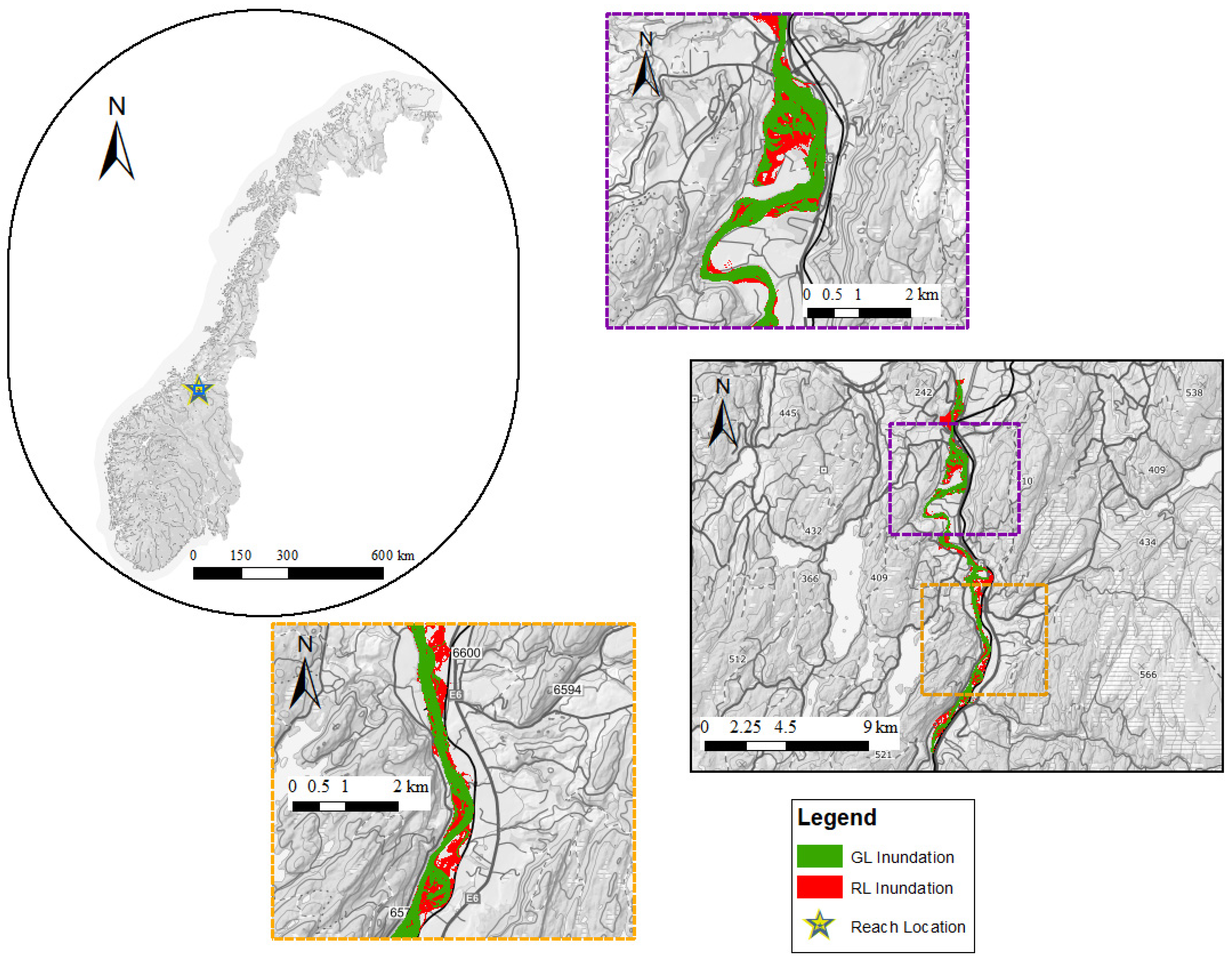
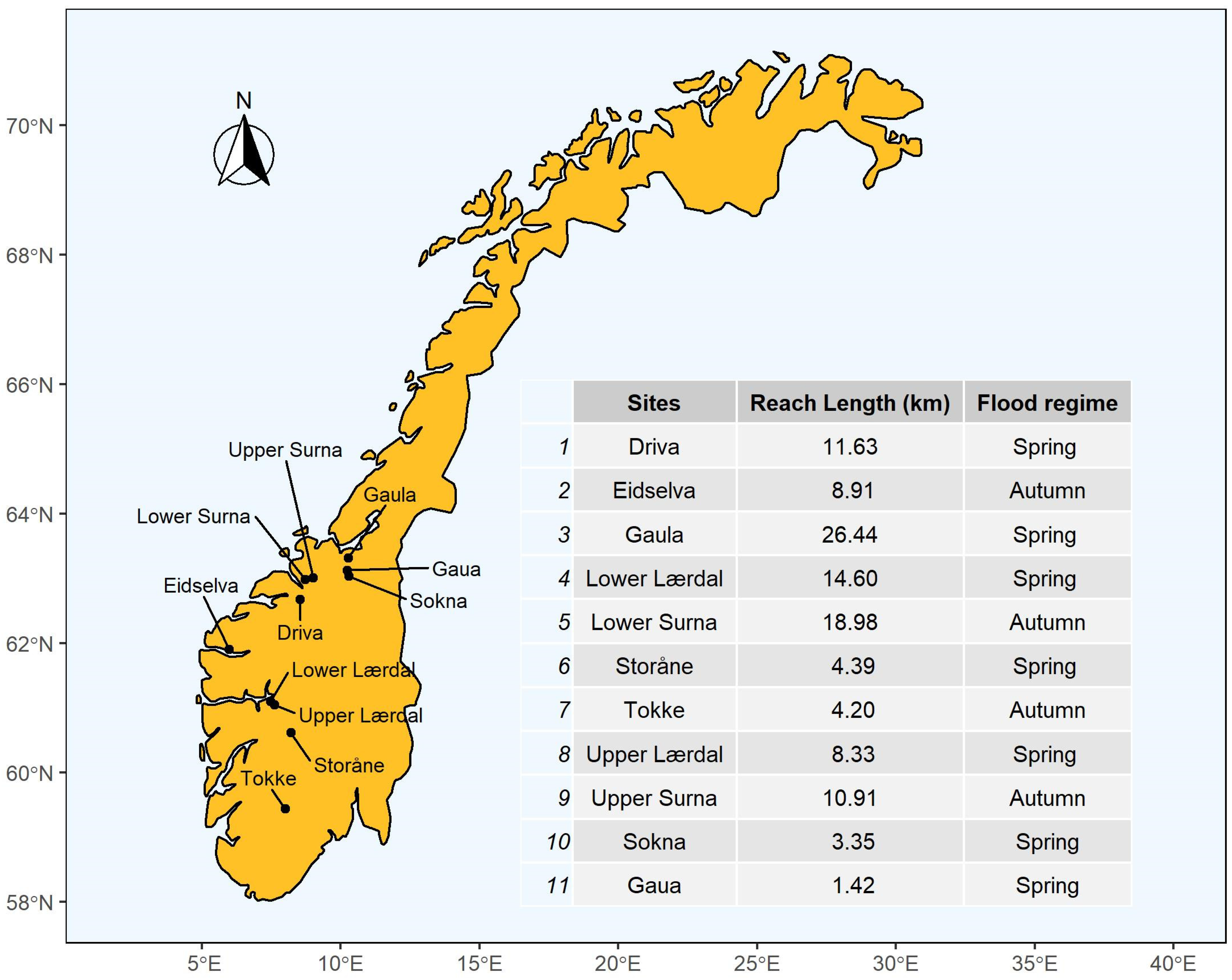
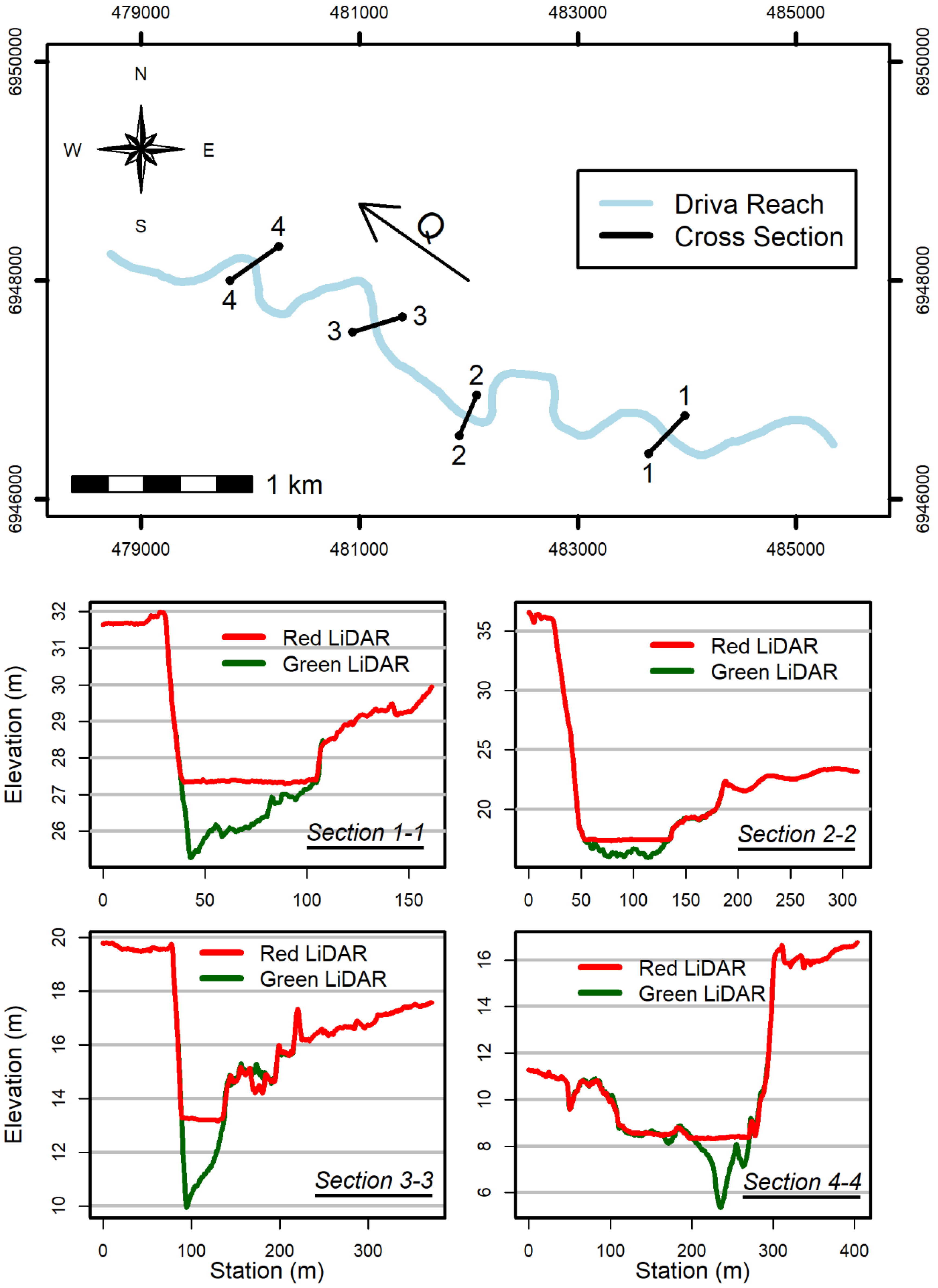
2.1. Study Sites
2.2. LiDAR Data
2.3. Flood Data
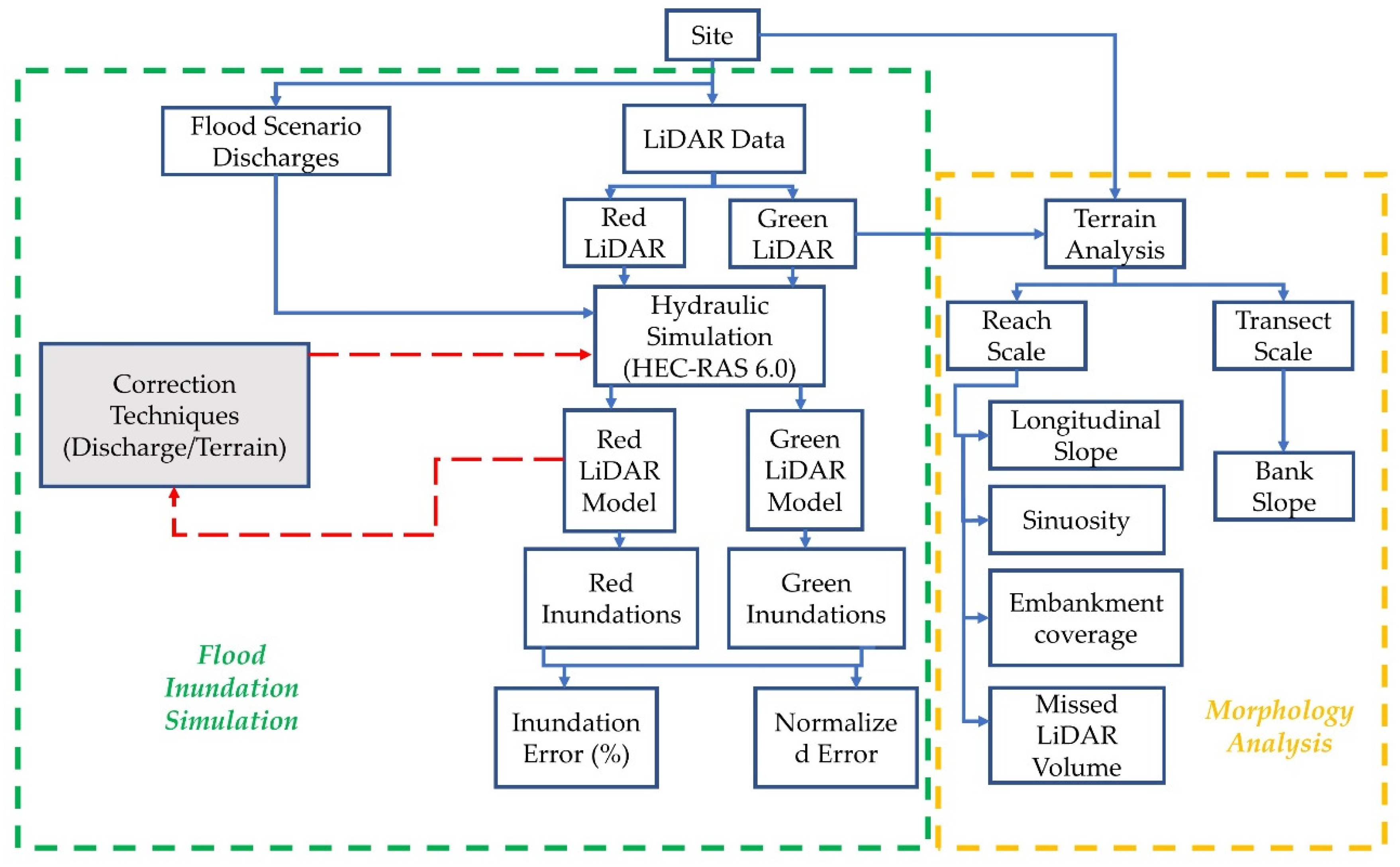
3. Methodology
3.1. DEM Generation for the LiDAR Models
3.2. Hydraulic Simulation
3.3. Terrain Analysis
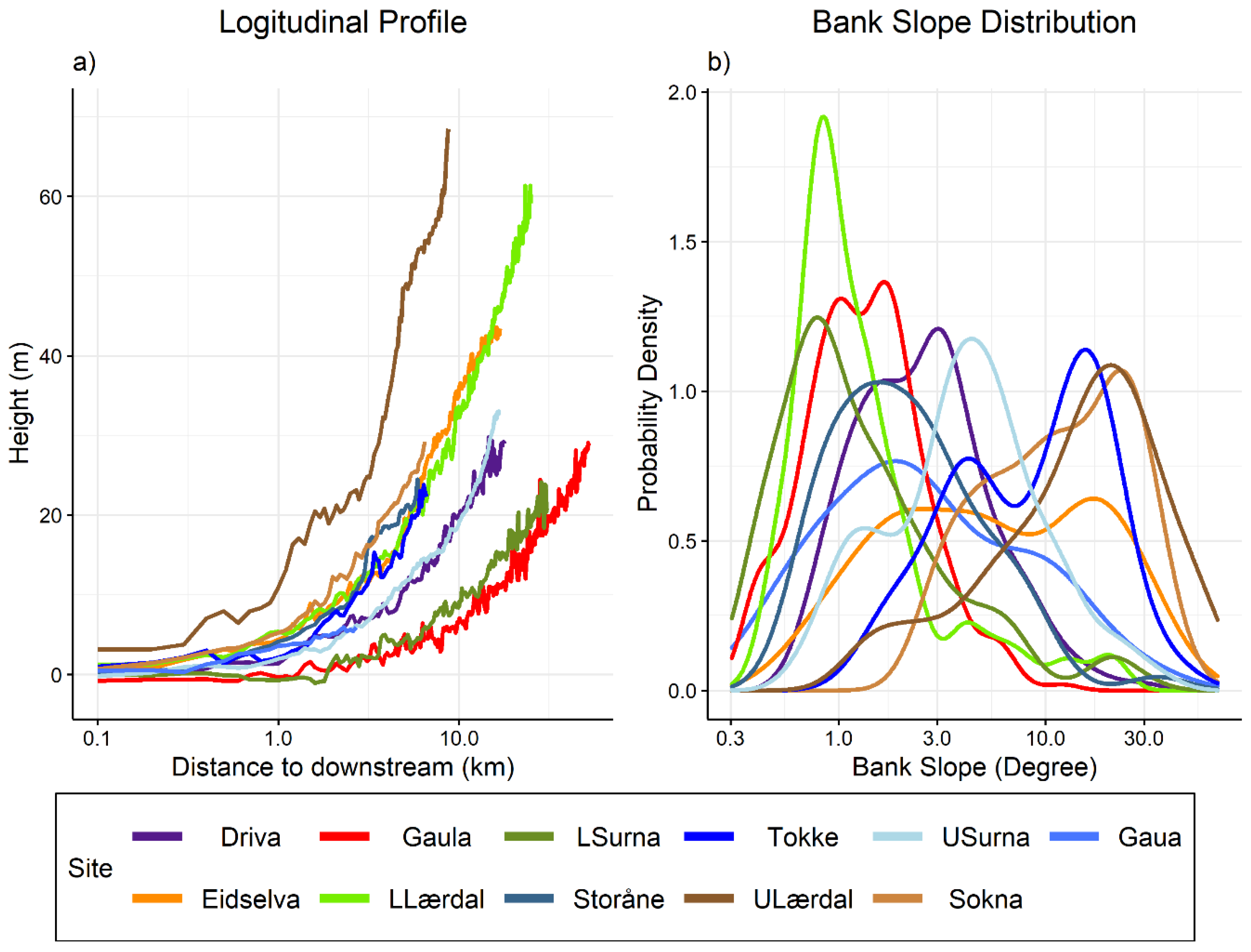
3.3.1. Longitudinal Slope, Sinuosity, and Flood Wall Coverage of the Reach
3.3.2. Missed LiDAR Volume
3.3.3. Bank Slope
3.4. Evaluation of the Flood Extents
3.5. Statistical Tests
3.6. Correction Methods
4. Results
4.1. Terrain Analysis Outputs
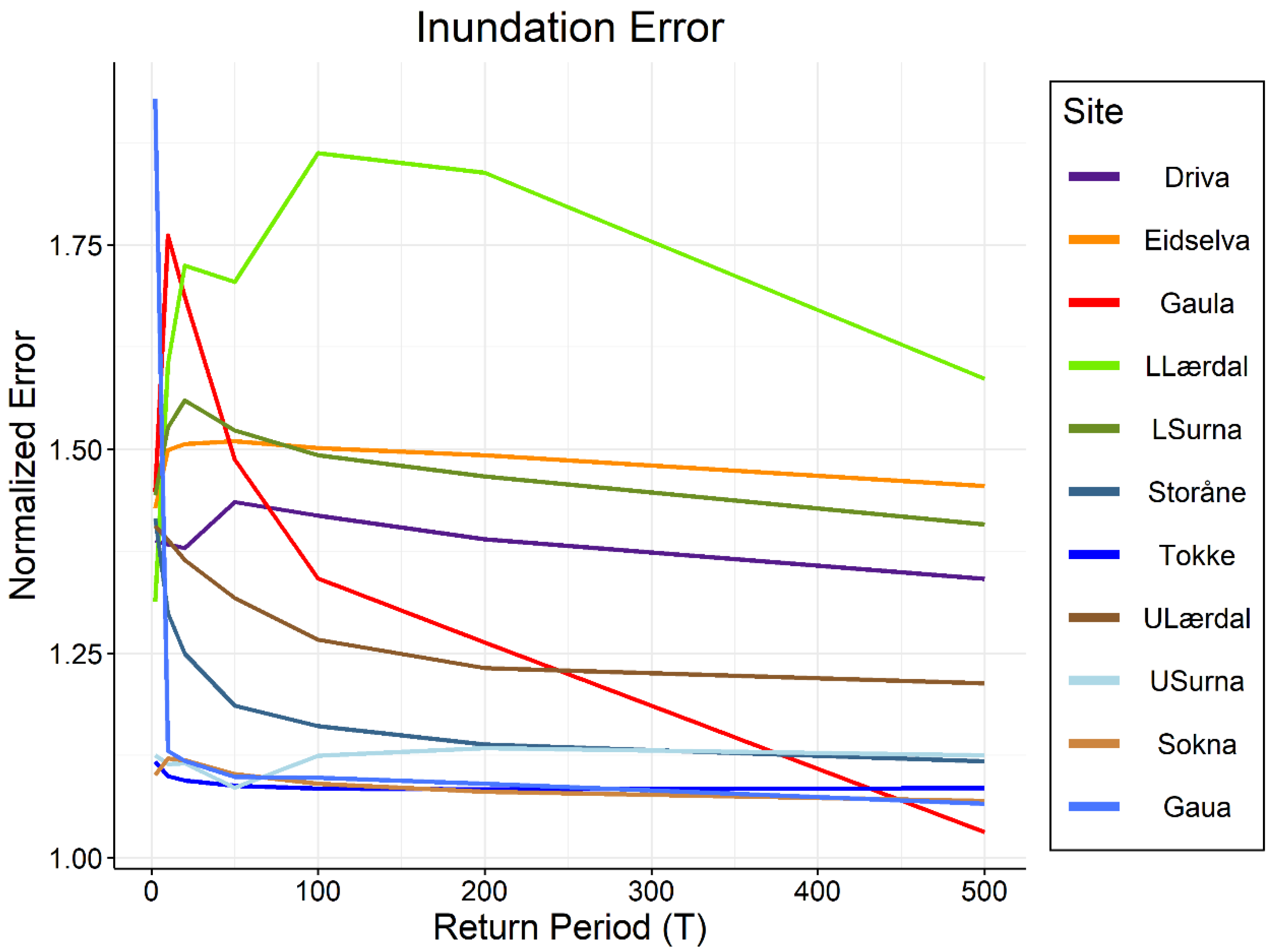
4.2. Inundation Error Development
4.3. Statistical Tests’ Outputs
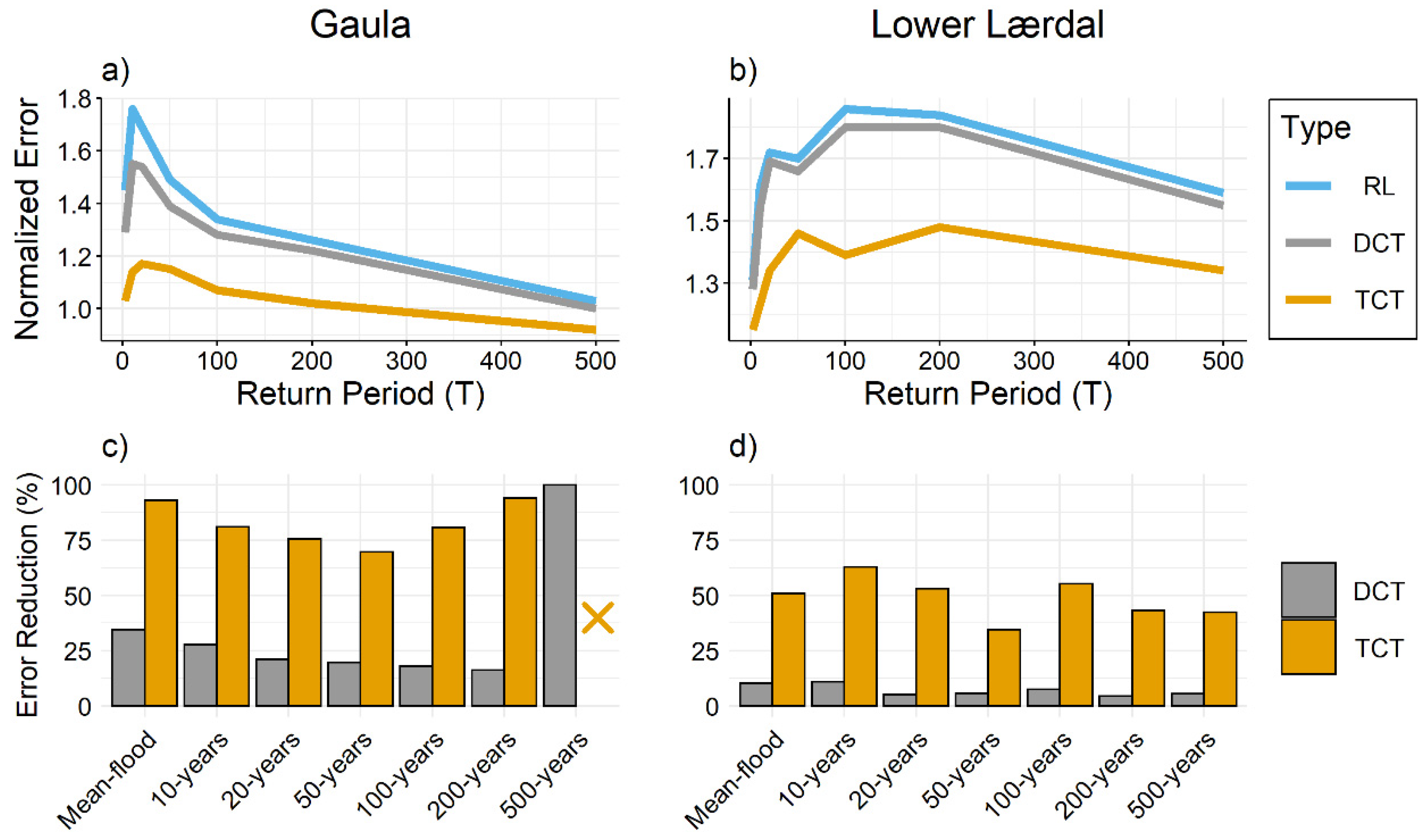
4.4. Correction Techniques Outputs
5. Discussion
5.1. Shape of the Inundation Error’s Curve
5.2. Level of the Inundation Error
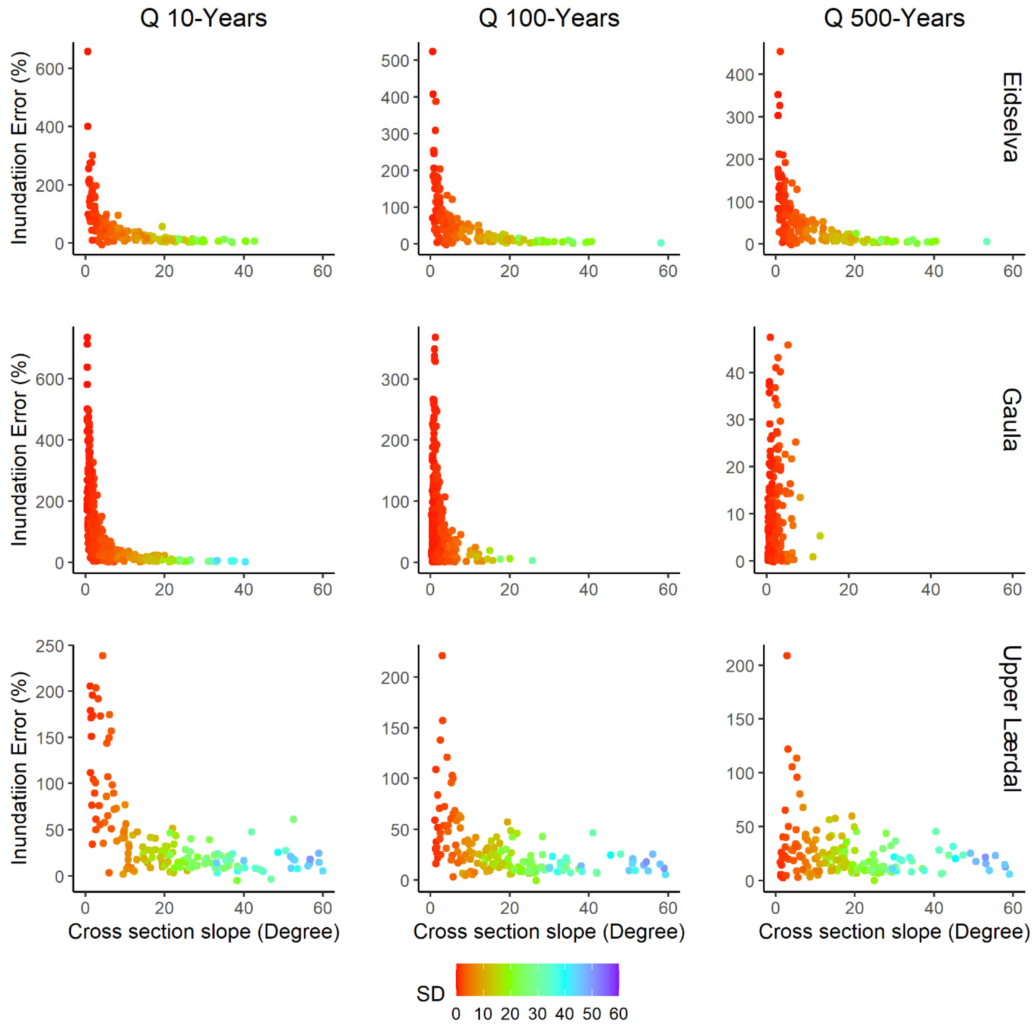
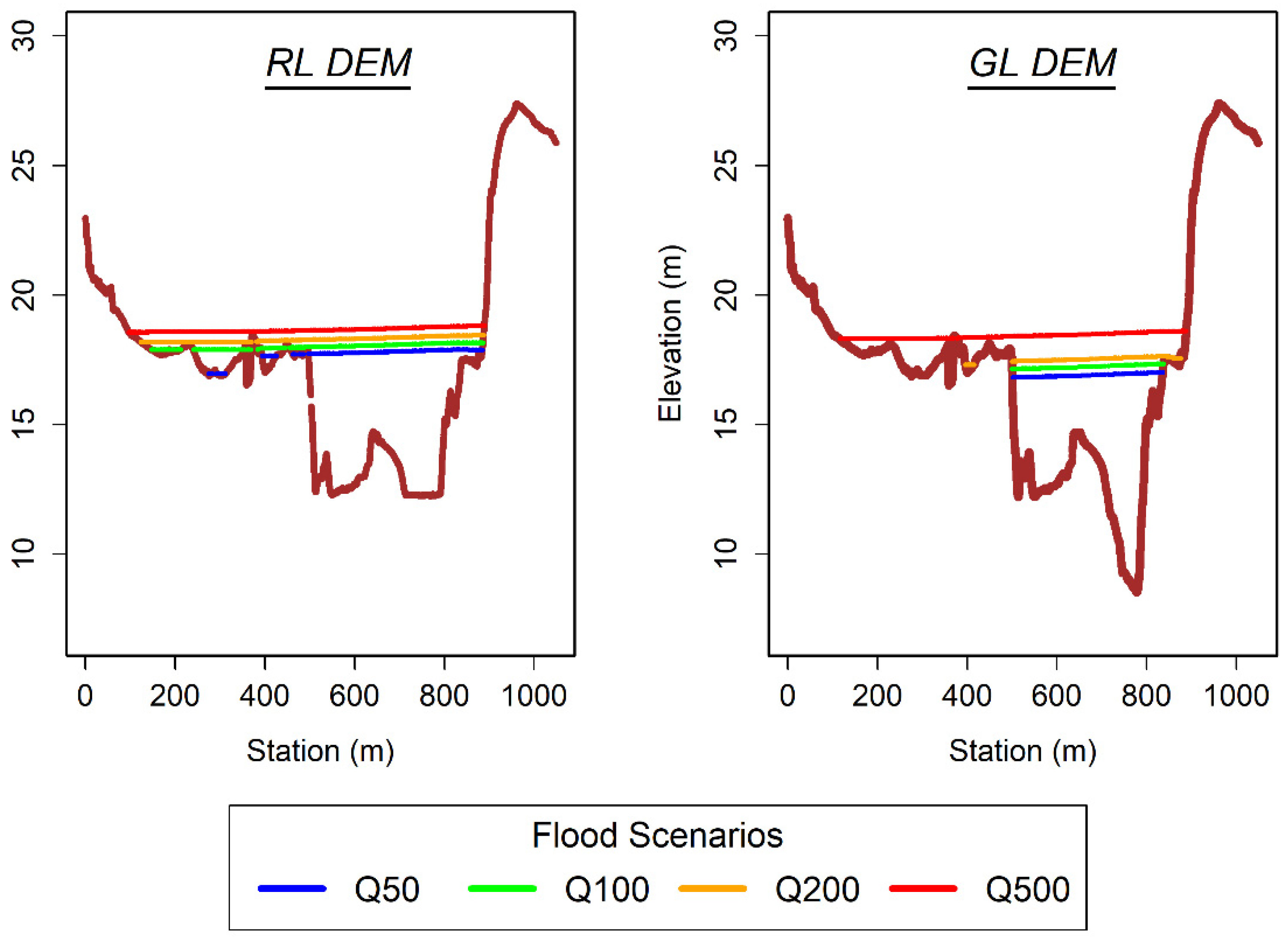
5.3. Inundation’s Error at Cross-Sectional Scales
5.4. Flood Model Correction
6. Conclusions
Author Contributions
Funding
Institutional Review Board Statement
Informed Consent Statement
Data Availability Statement
Acknowledgments
Conflicts of Interest
Appendix A

References
- Ciscar, J.C.; Iglesias, A.; Feyen, L.; Szabó, L.; Van Regemorter, D.; Amelung, B.; Nicholls, R.; Watkiss, P.; Christensen, O.B.; Dankers, R.; et al. Physical and economic consequences of climate change in Europe. Proc. Natl. Acad. Sci. USA 2011, 108, 2678–2683. [Google Scholar] [CrossRef] [PubMed] [Green Version]
- Christensen, J.H.; Christensen, O.B. Severe summertime flooding in Europe. Nature 2003, 421, 805–806. [Google Scholar] [CrossRef] [PubMed]
- Frei, C.; Schöll, R.; Fukutome, S.; Schmidli, J.; Vidale, P.L. Future change of precipitation extremes in Europe: Intercomparison of scenarios from regional climate models. J. Geophys. Res. Atmos. 2006, 111. [Google Scholar] [CrossRef] [Green Version]
- Blöschl, G.; Hall, J.; Parajka, J.; Perdigão, R.A.P.; Merz, B.; Arheimer, B.; Aronica, G.T.; Bilibashi, A.; Bonacci, O.; Borga, M.; et al. Changing climate shift timing of European floods. Science 2017, 357, 588–590. [Google Scholar] [CrossRef] [PubMed] [Green Version]
- Lawrence, D. Uncertainty introduced by flood frequency analysis in projections for changes in flood magnitudes under a future climate in Norway. J. Hydrol. Reg. Stud. 2020, 28, 100675. [Google Scholar] [CrossRef]
- Rözer, V.; Müller, M.; Bubeck, P.; Kienzler, S.; Thieken, A.; Pech, I.; Schröter, K.; Buchholz, O.; Kreibich, H. Coping with pluvial floods by private households. Water 2016, 8, 304. [Google Scholar] [CrossRef] [Green Version]
- Tanaka, T.; Kiyohara, K.; Tachikawa, Y. Comparison of fluvial and pluvial flood risk curves in urban cities derived from a large ensemble climate simulation dataset: A case study in Nagoya, Japan. J. Hydrol. 2020, 584, 124706. [Google Scholar] [CrossRef]
- Apel, H.; Martínez Trepat, O.; Nghia Hung, N.; Thi Chinh, D.; Merz, B.; Viet Dung, N. Combined fluvial and pluvial urban flood hazard analysis: Concept development and application to Can Tho city, Mekong Delta, Vietnam. Nat. Hazards Earth Syst. Sci. 2016, 16, 941–961. [Google Scholar] [CrossRef] [Green Version]
- Zurich Insurance Group. Three Common Types of Flood Explained; Zurich Insurance Group: Zurich, Switzerland, 2020; Available online: https://www.zurich.com/en/knowledge/topics/flood-and-water-damage/three-common-types-of-flood (accessed on 16 May 2021).
- U.S. Geological Survey. US GeoData Digital Elevation Models; U.S. Geological Survey: Reston, VA, USA, 2000; Fact Sheet.
- Muhadi, N.A.; Abdullah, A.F.; Bejo, S.K.; Mahadi, M.R.; Mijic, A. The use of LiDAR-derived DEM in flood applications: A review. Remote Sens. 2020, 12, 2308. [Google Scholar] [CrossRef]
- Jarihani, A.A.; Callow, J.N.; McVicar, T.R.; Van Niel, T.G.; Larsen, J.R. Satellite-derived Digital Elevation Model (DEM) selection, preparation and correction for hydrodynamic modelling in large, low-gradient and data-sparse catchments. J. Hydrol. 2015, 524, 489–506. [Google Scholar] [CrossRef]
- Hafezi, M.; Sahin, O.; Stewart, R.A.; Mackey, B. Creating a novel multi-layered integrative climate change adaptation planning approach using a systematic literature review. Sustainability 2018, 10, 4100. [Google Scholar] [CrossRef] [Green Version]
- Wang, Y.; Chen, A.S.; Fu, G.; Djordjević, S.; Zhang, C.; Savić, D.A. An integrated framework for high-resolution urban flood modelling considering multiple information sources and urban features. Environ. Model. Softw. 2018, 107, 85–95. [Google Scholar] [CrossRef]
- Lefsky, M.A.; Cohen, W.B.; Parker, G.G.; Harding, D.J. Lidar remote sensing for ecosystem studies. Bioscience 2002, 52, 19–30. [Google Scholar] [CrossRef]
- Dowman, I. Integration of LIDAR and IFSAR for mapping. Int. Arch. Photogramm. Remote Sens. 2004, 35, 90–100. [Google Scholar]
- Hodgson, M.E.; Jensen, J.R.; Schmidt, L.; Schill, S.; Davis, B. An evaluation of LIDAR- and IFSAR-derived digital elevation models in leaf-on conditions with USGS Level 1 and Level 2 DEMs. Remote Sens. Environ. 2003, 84, 295–308. [Google Scholar] [CrossRef]
- Bhuyian, M.N.M.; Kalyanapu, A. Accounting digital elevation uncertainty for flood consequence assessment. J. Flood Risk Manag. 2018, 11, S1051–S1062. [Google Scholar] [CrossRef]
- McClean, F.; Dawson, R.; Kilsby, C. Implications of Using Global Digital Elevation Models for Flood Risk Analysis in Cities. Water Resour. Res. 2020, 56, e2020WR028241. [Google Scholar] [CrossRef]
- Muthusamy, M.; Casado, M.R.; Butler, D.; Leinster, P. Understanding the effects of Digital Elevation Model resolution in urban fluvial flood modelling. J. Hydrol. 2021, 596, 126088. [Google Scholar] [CrossRef]
- Casas, A.; Benito, G.; Thorndycraft, V.R.; Rico, M. The topographic data source of digital terrain models as a key element in the accuracy of hydraulic flood modelling. Earth Surf. Processes Landf. 2006, 31, 444–456. [Google Scholar] [CrossRef]
- Bures, L.; Roub, R.; Sychova, P.; Gdulova, K.; Doubalova, J. Comparison of bathymetric data sources used in hydraulic modelling of floods. J. Flood Risk Manag. 2019, 12, e12495. [Google Scholar] [CrossRef] [Green Version]
- Choné, G.; Biron, P.M.; Buffin-Bélanger, T. Flood hazard mapping techniques with LiDAR in the absence of river bathymetry data. E3S Web Conf. 2018, 40, 06005. [Google Scholar] [CrossRef]
- Dey, S.; Saksena, S.; Merwade, V. Assessing the effect of different bathymetric models on hydraulic simulation of rivers in data sparse regions. J. Hydrol. 2019, 575, 838–851. [Google Scholar] [CrossRef]
- Reil, A.; Skoulikaris, C.; Alexandridis, T.K.; Roub, R. Evaluation of riverbed representation methods for one-dimensional flood hydraulics model. J. Flood Risk Manag. 2018, 11, 169–179. [Google Scholar] [CrossRef]
- Hilldale, R.C.; Raff, D. Assessing the ability of airborne LiDAR to map river bathymetry. Earth Surf. Processes Landf. 2008, 33, 773–783. [Google Scholar] [CrossRef]
- Irish, J.L.; Lillycrop, W.J. Scanning laser mapping of the coastal zone: The SHOALS system. ISPRS J. Photogramm. Remote Sens. 1999, 54, 123–129. [Google Scholar] [CrossRef]
- Kinzel, P.J.; Legleiter, C.J.; Nelson, J.M. Mapping River Bathymetry With a Small Footprint Green LiDAR: Applications and Challenges. J. Am. Water Resour. Assoc. 2013, 49, 183–204. [Google Scholar] [CrossRef]
- Mandlburger, G.; Hauer, C.; Wieser, M.; Pfeifer, N. Topo-Bathymetric LiDAR for Monitoring River Morphodynamics and Instream Habitats-A Case Study at the Pielach River. Remote Sens. 2015, 7, 6160–6195. [Google Scholar] [CrossRef] [Green Version]
- Breili, K.; Simpson, M.J.R.; Klokkervold, E.; Roaldsdotter Ravndal, O. High accuracy coastal flood mapping for Norway using LiDAR data. Nat. Hazards Earth Syst. Sci. Discuss. 2019, 20, 673–694. [Google Scholar] [CrossRef] [Green Version]
- Gottschalk, L.; Jensen, L.J.; Lundquist, D.; Solantie, R.; Tollan, A. Hydrologic regions in the Nordic countries. Nord. Hydrol. 1979, 10, 273–286. [Google Scholar] [CrossRef]
- Engeland, K.; Glad, P.; Hamududu, B.H.; Li, H.; Reitan, T.; Stenius, S. Lokal og Regional Flomfrekvensanalyse; Rapport nr. 10/2020; Norges Vassdrags-og Energidirektorat: Oslo, Norway, 2020; ISBN 9788241020148. Available online: https://publikasjoner.nve.no/rapport/2020/rapport2020_10.pdf (accessed on 3 January 2022).
- Brunner. Hydraulic Reference Manual; US Army Corps of Engineers: Washington, DC, USA, 1995; pp. 1–2. [Google Scholar]
- Cook, A.; Merwade, V. Effect of topographic data, geometric configuration and modeling approach on flood inundation mapping. J. Hydrol. 2009, 377, 131–142. [Google Scholar] [CrossRef]
- Jung, H.C.; Jasinski, M.; Kim, J.W.; Shum, C.K.; Bates, P.; Neal, J.; Lee, H.; Alsdorf, D. Calibration of two-dimensional floodplain modeling in the central Atchafalaya Basin Floodway System using SAR interferometry. Water Resour. Res. 2012, 48, 1–13. [Google Scholar] [CrossRef] [Green Version]
- Chow, V.T. Open Channel Hydraulics; McGraw-Hill: New York, NY, USA, 1959. [Google Scholar]
- Wei, T.; Simko, V. R Package “Corrplot”: Visualization of a Correlation Matrix. 2021. Available online: https://github.com/taiyun/corrplot (accessed on 10 May 2021).
- Fox, J.; Weisberg, S. An {R} Companion to Applied Regression, 3rd ed.; Sage: Thousand Oaks, CA, USA, 2019. [Google Scholar]
- Bradbrook, K.F.; Lane, S.N.; Waller, S.G.; Bates, P.D. Two dimensional diffusion wave modelling of flood inundation using a simplified channel representation. Int. J. River Basin Manag. 2004, 2, 211–223. [Google Scholar] [CrossRef]
- Rosgen, D.L. A classification of natural rivers. Catena 1994, 22, 169–199. [Google Scholar] [CrossRef] [Green Version]
- Hassan, M.A.; Reid, I. The influence of microform bed roughness elements on flow and sediment transport in gravel bed rivers. Earth Surf. Process. Landf. 1990, 15, 739–750. [Google Scholar] [CrossRef]
- Płaczkowska, E.; Krzemień, K. Natural conditions of coarse bedload transport in headwater catchments (Western Tatras, Poland). Geogr. Ann. Ser. A Phys. Geogr. 2018, 100, 370–387. [Google Scholar] [CrossRef]


| Site | Catchment Area (km2) | Mean Discharge (m3/s) | RL Resolution (m) | RL Point Density (Points/m2) | RL Flow (m3/s) | GL Resolution (m) | GL Point Density (Points/m2) | GL Laser Scanner |
|---|---|---|---|---|---|---|---|---|
| Driva | 2436 | 63.6 | 0.5 | 2 | 74 | 0.25 | 4 | Optech Titan |
| Eidselva | 386 | 23.4 | 0.25 | 5 | 17.6 | 0.25 | 4 | Optech Titan |
| Gaula | 3086 | 83.3 | 0.25 | 6 | 146 | 0.25 | 5 | Optech Titan |
| Lower Lærdal | 994 | 30.7 | 0.5 | 2 | 14 | 0.25 | 5 | VQ880-G (RIEGL) |
| Lower Surna | 910 | 40.6 | 0.5 | 2 | 20 | 0.5 | NA | VQ880-G (RIEGL) |
| Storåne 1 | 770 | 24.5 | 0.25 | 5 | 6.8 | 0.2 | 20 | VQ880-G (RIEGL) |
| 35.9 | ||||||||
| Tokke | 2332 | 89.5 | 0.25 | 5 | 22.9 | 0.25 | 20 | VQ880-G (RIEGL) |
| Upper Lærdal 2 | 750 | 23.0 | 0.25 | 5 | 26 | 0.25 | 5 | VQ880-G (RIEGL) |
| 0.5 | 2 | 13 | 0.25 | 5 | ||||
| Upper Surna | 445 | 17.4 | 0.5 | 2 | NA | 0.5 | NA | VQ880-G (RIEGL) |
| Sokna | 564 | 13.0 | 0.25 | 5 | 15 | 0.25 | 5 | Optech Titan |
| Gaua | 84.6 | 2.0 | 0.25 | 6 | 1.5 | 0.25 | 5 | Optech Titan |
| Site | Q M | Q 10 | Q 20 | Q 50 | Q 100 | Q 200 | Q 500 |
|---|---|---|---|---|---|---|---|
| Driva | 545 | 725 | 795 | 885 | 960 | 1025 | 1115 |
| Eidselva | 66 | 86 | 93 | 101 | 107 | 112 | 118 |
| Gaula | 1041 | 1551 | 1800 | 2144 | 2404 | 2685 | 3070 |
| Lower Lærdal | 235 | 380 | 470 | 570 | 700 | 800 | 890 |
| Lower Surna | 229 | 342 | 391 | 454 | 501 | 549 | 613 |
| Storåne * | 196 | 290 | 327 | 374 | 410 | 446 | 493 |
| Tokke | 204 | 289 | 323 | 366 | 406 | 443 | 492 |
| Upper Lærdal | 215 | 310 | 350 | 398 | 452 | 495 | 538 |
| Upper Surna | 171 | 230 | 254 | 284 | 306 | 328 | 355 |
| Sokna * | 125 | 194 | 221 | 257 | 284 | 311 | 347 |
| Gaua * | 21.9 | 34.5 | 39.5 | 46.1 | 51.1 | 56.2 | 63.1 |
| Site | Missed LiDAR Volume (m3/m) | Slope (%) | Sinuosity | Flood Protection Coverage (%) | Mean Bank’s Slope (Degrees) |
|---|---|---|---|---|---|
| Driva | 17 | 0.29 | 1.37 | 24 | 2.97 |
| Eidselva | 26 | 0.49 | 1.84 | 11 | 9.88 |
| Gaula | 141 | 0.12 | 1.33 | 62 | 1.66 |
| Lower Lærdal | 8 | 0.42 | 1.63 | 72 | 2.15 |
| Lower Surna | 36 | 0.14 | 1.27 | 25 | 2.41 |
| Storåne | 4 | 0.57 | 1.25 | 0 | 3.25 |
| Tokke | 27 | 0.51 | 1.29 | 15 | 11.24 |
| Upper Lærdal | 5 | 1.90 | 1.35 | 3 | 19.54 |
| Upper Surna | 5 | 0.36 | 1.14 | 20 | 5.82 |
| Sokna | 15 | 0.92 | 1.15 | 39 | 15.01 |
| Gaua | 5 | 0.46 | 1.14 | 15 | 4.76 |
Publisher’s Note: MDPI stays neutral with regard to jurisdictional claims in published maps and institutional affiliations. |
© 2022 by the authors. Licensee MDPI, Basel, Switzerland. This article is an open access article distributed under the terms and conditions of the Creative Commons Attribution (CC BY) license (https://creativecommons.org/licenses/by/4.0/).
Share and Cite
Awadallah, M.O.M.; Juárez, A.; Alfredsen, K. Comparison between Topographic and Bathymetric LiDAR Terrain Models in Flood Inundation Estimations. Remote Sens. 2022, 14, 227. https://doi.org/10.3390/rs14010227
Awadallah MOM, Juárez A, Alfredsen K. Comparison between Topographic and Bathymetric LiDAR Terrain Models in Flood Inundation Estimations. Remote Sensing. 2022; 14(1):227. https://doi.org/10.3390/rs14010227
Chicago/Turabian StyleAwadallah, Mahmoud Omer Mahmoud, Ana Juárez, and Knut Alfredsen. 2022. "Comparison between Topographic and Bathymetric LiDAR Terrain Models in Flood Inundation Estimations" Remote Sensing 14, no. 1: 227. https://doi.org/10.3390/rs14010227
APA StyleAwadallah, M. O. M., Juárez, A., & Alfredsen, K. (2022). Comparison between Topographic and Bathymetric LiDAR Terrain Models in Flood Inundation Estimations. Remote Sensing, 14(1), 227. https://doi.org/10.3390/rs14010227