Article

Updated GOES-13 Heliosat-2 Method for Global Horizontal Irradiation in the Americas

ESPACE-DEV, Univ Guyane & Univ Réunion & Univ Montpellier & IRD & Univ Antilles, 97300 Cayennez, France
*
Author to whom correspondence should be addressed.
These authors contributed equally to this work.
Remote Sens. 2022, 14(1), 224; https://doi.org/10.3390/rs14010224
Submission received: 26 October 2021 / Revised: 6 December 2021 / Accepted: 7 December 2021 / Published: 4 January 2022

Abstract

:
Increasing the utilization of renewable energy is at the center of most sustainability policies. Solar energy is the most abundant resource of this type on Earth, and optimizing its use requires the optimal estimation of surface solar irradiation. Heliosat-2 is one of the most popular methods of global horizontal irradiation (GHI) estimation. Originally developed for the Meteosat satellite, Heliosat-2 has been modified in previous work to deal with GOES-13 data and named here GOES_H2. This model has been validated through the computation of indicators and irradiation maps for the Guiana Shield. This article proposes an improved version of GOES_H2, which has been combined with a radiative transfer parameterization (RTP) and the McClear clear-sky model (MC). This new version, hereafter designated RTP_MC_GOES_H2, was tested on eight stations from the Baseline Surface Radiation Network, located in North and South America, and covered by GOES-13. RTP_MC_GOES_H2 improves the hourly GHI estimates independently of the type of sky. This improvement is independent of the climate, no matter the station, the RTP_MC_GOES_H2 gives better results of MBE and RMSE than the original GOES_H2 method. Indeed, the MBE and RMSE values, respectively, change from 11.93 % to 2.42 % and 23.24 % to 18.24 % for North America and from 4.35 % to 1.79 % and 19.97 % to 17.37 for South America. Moreover, the flexibility of the method may allow to improve results in the presence of snow cover and rainy/variable weather. Furthermore, RTP_MC_GOES_H2 results outperform or equalize those of other operational models.

1. Introduction

In light of the energy transition challenge, electricity production using renewable energy has received growing interest [1,2]. For instance, the Energy Sector Management Assistance Program shows that the annual photovoltaic power potential is quite high for most countries [3]. However, maximizing solar radiation exploitation requires managing surface irradiation, namely, global horizontal irradiation (GHI) [4,5]. These data can be obtained in two main ways: in situ measurements [6] and estimation using satellite images [7]. Measurements are captured by instruments that require specific installation and continuous calibration and maintenance [8]. As a consequence, satellite-based estimation is receiving increasing interest [9].
Surface irradiation estimation via satellite falls into two main categories: direct and indirect models. Direct approaches use a radiative transfer model to evaluate the radiative loss between the top-of-atmosphere and the surface [10,11]. Indirect hybrid approaches combine physical models and empirical parameters to facilitate the estimation procedure [12,13]. Hence, while approaches in the first group are complex and time-consuming, and require atmospheric information [14], those in the second category are simpler and, thus, attractive.
Among the direct approaches, we can cite the physical solar model (PSM) developed by the National Renewable Energy Laboratory (NREL) for the creation of the National Solar Radiation Database (NSRDB), which provides irradiation data for North- and (the northern part of) South America [15]. The model is based on the introduction of cloud transmittances and reflectances parameterized by data provided by satellite (as optical thickness) for cloudy-sky condition coupled to the REST-2 clear-sky model [16]. GHI data are provided at a spatial resolution of 4 km at a time step up to one hour. Moreover, the NASA Prediction Of Worldwide Energy Resources (POWER) [17] provides hourly GHI data for worldwide at spatial resolution of 50 km. Another approach is the Heliosat-4 method [18] based on two models: the McClear clear-sky model [19] for the estimation of clear-sky irradiation and the McCloud model [20] to assess the attenuation due to clouds. The two models are based on the use of abaci to tackle the computation cost related to this type of approach. GHI data are provided for Meteosat satellite coverage at spatial resolution of 3 km at time-step up to one hour.
Concerning hybrid methods, let us cite the BRASIL-SR [13] that combines radiative transfer model and empirical method for estimating cloud cover to give solar irradiation estimation in Brazil at a spatial resolution of 3 × 5 km at a time-step of 30 min. There is also Heliosat-3 [21] based on the empirical estimation of a cloud index that provides irradiation estimates for Meteosat coverage at spatial resolution of 3 km. The Heliosat-3 clear-sky model is the solar irradiance scheme (SOLIS) [22] based on a radiative transfer model. Let us also mention Heliosat-2 (H2), based on the use of a cloud index and with the same spatial configurations than Heliosat-3. H2 is performed with the European Solar Radiation Atlas (ESRA) clear-sky model only, based on physical equations and empirical configurations. ESRA is based on Linke turbidity, which is a fixed value for each pixel of size 0.083 ° × 0.083 °, and each month [23]. Within the Heliosat family, only Heliosat-2 codes are provided and open access. Hence, easy to optimize for specific regions.
Reference [19] introduced a new clear-sky model, namely, the McClear clear-sky model. It relies on a radiative transfer model and regularly updated data. Hence, while ESRA model [23] uses empirical assumptions, the McClear model is based on a fully physical approach. The introduction of this clear-sky model shows improvements, in comparison to the ESRA model, for clear skies irradiance giving RMSE values up to 3% for hourly estimates. Conversely, several studies have shown that H2 estimates under cloudy skies are less accurate than those under clear sky [7,24].
The original H2 model was designed to work with data from the visible band of the geostationary meteorological satellite, Meteosat, that covers Africa, Europe, the Middle East, and the western part of South America. Studies [7,25,26] have validated the approach in the geographical area covered by the satellite, however, due to its location nadir, Meteosat is affected by a poor viewing angle at the western edges of its spatial coverage inducing less accurate GHI estimates. Therefore, the model needs to be optimized for other satellites that cover the American continent.
Thus in reference [24], the original H2 method based on ESRA model was optimized so that Meteosat images could be replaced by GOES images (GOES stands for geostationary operational environment satellite), which covers South America and most of North America. This method is named GOES_H2 in this paper. The method was validated in French Guiana by comparing estimated hourly irradiation to in situ data. A subsequent work [27] carried out spatial GHI estimation and spatiotemporal indicator computations in the Guiana Shield in South America; the authors compared GOES_H2 estimates with H2 estimates using Meteosat images and demonstrated that GOES_H2 outperforms H2 method under all types of skies in French Guiana.
Located in the intertropical zone, French Guiana is subject to random and regular cover, moreover, in [24], authors pointed out that GOES_H2 method gives less good performance under cloudy skies than under clear skies. Hence, in [28], a cloudy-sky irradiation parameter was introduced to deal with cloud cover in tropical climates, particularly in French Guiana. The introduced radiative transfer parameterization has shown promising results under cloudy skies [28].
The first objective of this paper is to propose an updated version of the GOES_H2 that would be efficient under all types of skies: cloudy and clear. This would be done by replacing the ESRA model by the McClear model in order to benefit from fully physical approach of the clear-sky modeling. In addition, by introducing a radiative transfer parameterization so that cloudy-sky irradiation would be efficiently taken into account and improve GHI estimates.
GHI estimation methods on the American continent are, either regional methods (BRASIL-SR [13], Heliosat family [7,20,22], PSM [15]), either methods with low spatial resolution (POWER [17]), which limits the availability of GHI data in this area. Hence, the second objective of this article is to propose the updated method named hereafter RTP_MC_GOES_H2 for providing accurate GHI estimates at fine resolution (1 × 1 km) and for GOES-13 spatial coverage ( 81.32 °N to 81.32 °S and 6.29 °E to 156.29 °W). Therefore, RTP_MC_GOES_H2 was validated on different areas of the American continent. GHI estimation was here performed on stations of the Baseline Surface Radiation Network (BSRN). The BSRN [29] is a global network of radiation sensors with high accuracy. Eight stations were chosen in North (four) and South (four) America to match the geographical coverage of GOES-13. Moreover, to assess the performance of the method, RTP_MC_GOES_H2 estimates were compared to other operational models (Heliosat-4, POWER and PSM) estimates.
Herein, the method RTP_MC_GOES_H2 and the data are first presented. Then, the results obtained with RTP_MC_GOES_H2 method are compared with those obtained with GOES_H2 and to results from free access web services generated by other methods. These results are then discussed before ending with conclusions.

2. Materials and Methods

2.1. GOES-13 Data

The geostationary operational environment satellite of the second generation, GOES-13, also known as GOES-N [30], was located at 75°W above the Equator from April 2010 to December 2017. The satellite had one band in the visible range centered on 0.63 μ m for a spatial resolution of 1 × 1 km.
Moreover, GOES-13 covered the considered regions twice per hour at approximately minutes 15 and 45.
GOES-13 images from 1 January to 31 December 2015, were downloaded.
The National Oceanic and Atmospheric Administration provided GOES-13 images via the Comprehensive Large-Array Stewardship System. The downloaded data were encoded in 16 bits.

GOES-13 Image Requests per Region

The Comprehensive Large-Array Stewardship System allows GOES-13 data to be downloaded for specific regions. Thus, instead of downloading full disk images, requests were made for the regions of interest.
In particular, the BSRN stations located in South America cover a large area. Hence, for computational efficiency, three areas were defined for downloading GOES-13 images:
  • North America: 99° W and 32° N to 86° W and 42° N.
  • South America:
    Brasilia and Petrolina stations: 50° W and 8°S to 38° W and 18° S;
    Florianopolis and São Martinho da Serra stations: 56° W and 32° S to 46° W and 25° S.
The details of the stations are given in Section 2.3.

2.2. Description of the RTP_MC_GOES_H2 Method

2.2.1. The Original GOES_H2 Method

H2 is a hybrid model in which the key step is the computation of a cloud index, n, where n is a factor that quantifies the cloud cover above the specific area of interest. The operating principle is that cloudiness affects the solar irradiation that reaches the surface. Hence, the surface irradiation is effectively estimated by assessing the clearness of the sky. Thus, the model describes a method that, starting from digital counts, allows the estimation of n and then the global horizontal irradiation. The principal steps are described in the following.
GOES images were downloaded and converted into digital counts in 10 bits, followed by calibration for radiance. The best method is provided by the National Aeronautics and Space Administration (NASA) [31]:
L = ( g 3 · d 3 + g 2 · d 2 + g 1 · d + g 0 ) · ( CN 10 CN 0 )
where L is radiance in W/(m 2 .sr) with sr standing for the steradian unit; d the number of days since launch; g 0 is the initial gain; g 1 , g 2 and g 3 are, respectively, the first-, second-, and third-order polynomial terms of the gain trend that account for the sensor degradation since the launch; CN 10 and CN 0 , are, respectively, the digital counts in 10 bits and an offset (https://www-pm.larc.nasa.gov/cgi-bin/site/showdoc?mnemonic=SAT_CALIB_USER, accessed on 6 December 2021). For further details about the calibration, readers are redirected to [24].
The next step is to convert radiance into reflectance values through:
ρ sat = π L I 0 sat · ε · cos ( θ s )
where ρ sat is the satellite-derived reflectance, I 0 sat is total irradiance in the visible channel of the GOES-13 satellite (W/m 2 ), ε is the Earth–Sun distance correction factor and θ s is the solar zenith angle.
Apparent albedo, ρ , is deduced from reflectance values using:
ρ = ρ sat ρ atm ( θ s , θ v , ψ ) T ( θ s ) · T ( θ v )
where ρ atm is the apparent albedo of the atmosphere, θ v and ψ are the satellite viewing angle and the difference between the sun and satellite azimuth angles, respectively, and T ( θ s ) and T ( θ v ) are the downward and upward transmittances, respectively.
A key step in the H2 method is the computation of a cloud index, n, which allows the quantification of the cloudiness of the sky, the formula for which is:
n = ρ ρ g ρ c ρ g
where ρ c and ρ g are the cloud and ground albedo, respectively. The ground albedo is chosen as the second minimum of the albedo in a time range, which, in this study, is a month. The second minimum is selected instead of the absolute minimum to avoid, among other issues, values generated by undetected defects in satellite images. Different methods have been proposed for the cloud albedo computation [24]; however, in this study, the original method introduced in [7] was used. The cloud albedo has been defined as the typical value for the brightest clouds. This value is quite difficult to estimate. The authors of [32] proposed an approach based on the computation of an effective cloud albedo ( ρ eff ) using the sun zenith angle.
ρ c = ρ eff ρ atm ( θ s , θ v , ψ ) T ( θ s ) · T ( θ v )
with
ρ eff = 0.85 0.13 · 1 exp 4 cos ( θ s ) 5
Empirical studies allow the computation of a clear-sky index, K c , based on the cloud index [7]:
n 0.2 K c = 1.2 0.2 < n 0.8 K c = 1 n 0.8 < n 1.1 K c = 2.0667 3.6667 n + 1.6667 n 2 1.1 < n K c = 0.05
Finally, an estimate of the global horizontal irradiation is given by:
GHI = G c · K c
where G c is the clear-sky irradiation—the irradiation that would reach the surface if the atmosphere were cloud-free—whose computation is discussed in the following part.

2.2.2. The MC_GOES_H2 Method

The European Solar Radiation Atlas (ESRA) [23] is the clear-sky model used in the original H2. It is a hybrid approach, combining both physical equations and empirical considerations, based on the Linke turbidity factor.
The Linke turbidity factor aims to quantify the attenuation of the radiation as it passes through the atmosphere [33]. An important problem with this factor is that it is considered fixed for each month. Hence, it does not consider changes in the atmosphere that occur in the same month based on geographical position, climate, etc.
Therefore, a new clear-sky model, namely, the McClear model, was proposed in a previous study [19] using recent results obtained through the Monitoring Atmosphere Composition and Climate (MACC) projects. The model is purported to more rapidly reproduce irradiation estimations obtained by a radiative transfer model by using look-up tables.
The McClear model is entirely physical and meteorological input data are continuously updated every three hours. Indeed, its inputs include atmospheric composition information provided by MACC models that use satellites and in situ data.
Clear-sky irradiation data are available at different time steps through the Copernicus Atmosphere Monitoring Service (CAMS) via a dedicated web interface [34]. In this study, the chosen time step is 1 min at download. Hence, to obtain the clear-sky irradiation every 30 min in the given interval, the integral (sum) of data was calculated on an interval of 30 min centered on the time of satellite acquisition at the corresponding point.
Let us name the MC_GOES_H2 the GOES_H2 method with the use of the McClear clear-sky model.

2.2.3. The RTP_MC_GOES_H2 Method

The H2 method is known to be less accurate for solar surface irradiation estimation under cloud cover. Furthermore, the thicker the clouds, the more difficult it is to estimate the irradiation. Indeed, in [7], the authors show that H2 gives less accurate estimations under cloudy skies in Europe and in [24], the authors have the same conclusions with a study in French Guiana using GOES_H2.
To overcome this issue, reference [28] proposed a modification, for tropical climate, of the equation of global horizontal irradiation (8) by combining clear- and cloudy-sky irradiation terms. Then, the equation for global horizontal irradiation becomes:
GHI = K c · G c + n · G b
The main objective was to improve GHI estimations in French Guiana, a region subject to significant cloud coverage, without negatively affecting clear-sky estimations or being time-consuming. Our work aims to generalize this approach to all types of climates and show that the GHI estimation is improved under all skies.
Based on the work by [35], the cloudy-sky radiative transfer parameterization (RTP) term, namely, G b , is written as:
G b = G c · 1 ρ eff α c 1 ρ eff · ρ g
where α c is cloud absorption (unitless). Radiative transfer models are the best models to estimate this term; however, to allow near-real-time estimation, a linear approximation function of the effective albedo (6) is proposed:
α c = a · ρ eff
The slope a is the one to be tuned. Authors in [36] propose to choose the value of coefficient a (11) between 0.04 and 0.17 . For our study, different values were tested, and the best results, presented hereafter, were obtained with a = 0.085 .
RTP_MC_GOES_H2 is an updated method that combines the H2 algorithm optimized for GOES-13 data [24] with the McClear clear-sky model [19] and a RTP term.
A flowchart of the methods is presented in Figure 1.

2.3. Choice of Ground Stations

The baseline surface radiation network is a global network of radiation measurement instruments [29]. The network allows the acquisition of surface solar irradiation measurements for stations that belong to it. However, maintaining the instruments is not one of its activities. This network is the best database of in situ data: the stations are chosen after rigorous screening.
Eight stations in the BSRN network were considered for this work. First, only stations located in America are relevant for our work since the objective is to validate the RTP_MC_GOES_H2 method in the geographical areas covered by the satellite. Second, we decided to analyze an entire year, so only stations that were active throughout this period were considered. Thus, eight stations were chosen: four in North America and four in South America for the year 2015. That year was chosen because, for all stations but one, measured data were available for all months. In North America, the stations are located in Oklahoma (Billings and Southern Great Plains), Illinois (Bondville), and Mississippi (Goodwin Creek). In South America, only four stations were available for the study period, all of which are in Brazil and located in Brasilia City, South Atlantic Ocean (Florianopolis), Petrolina, and São Martinho da Serra. The stations’ information is summarized in Table 1.
The selected stations in North America are in UTC-6, and those in South America are in UTC-3.
Only data for which the cosine of the sun zenith angle is greater than zero are selected to discard the ones for which the sun is completely low in the sky. The study is pursued in all skies condition.
A quality control on extreme values was made for the extreme values according to [37] and the solar radiation Data (SoDa) website (solar radiation data. http://soda-pro.com/, accessed on 6 December 2021). Measured hourly surface irradiation was considered valid when:
0.03 · G TOA < GHI < min ( 1.2 · I 0 ) , 1.5 · I 0 · cos ( θ s ) 1.2
where G TOA is the top-of-atmosphere hourly irradiation, θ s is the sun zenith angle and I 0 the solar constant (1367 W m 2 ).

Climate

Here, we used the Köppen Geiger climate classification [38]. This system classifies climates worldwide by using names containing two or three letters. The three letters refer to the main climate, precipitation information, and temperature, respectively.
The stations are grouped into three types of climates: Aw, BSh, and Cfa. Aw corresponds to an equatorial Savanna climate with dry winters and applies to the Brasilia station. BSh is a steppe climate with hot and arid temperatures (that is, the annual temperature is greater than 18 °C) and applies to the Petrolina station. Cfa is a warm, very humid climate with hot summers (the maximum temperature is greater than 22 °C); the Billings, Bondville, Florianopolis, Goodwin Creek, São Martinho da Serra and Southern Great Plains stations are situated in this type of climate.

2.4. Configurations

Data are considered valid for the study if both BSRN measurements and estimations are available. That is, data are treated as missing if either the in situ measurement or estimation is unavailable. A missing estimation is encountered when no satellite image is available or the image is corrupted at the station position.
A general function is the computation of the hourly estimate based on the estimates available per hour. As two acquisitions are available per hour, two surface irradiation estimations should be available for each hour. Consequently, the hourly estimate is the sum of the two 30-min estimates for the previous hour; that is,
GHI h = GHI 15 h 1 + GHI 45 h 1
where GHI 15 h 1 is the mean irradiation computed for a 30-min time range, centered on the acquisition at minute 15 of h 1 ; the same applies to GHI 45 h 1 but at minute 45.
The meteorological data (rainfall, snowfall, and temperature) [39] used in the below data analysis were provided by the Modern-Era Retrospective analysis for Research and Applications, Version 2 [40], and are available from the SoDa website (http://www.soda-pro.com/web-services/meteo-data/merra, accessed on 6 December 2021).

2.5. Metrics

Three metrics were computed to validate the estimations compared to the in situ measurements: the mean bias error (MBE), the root-mean-square error (RMSE), and r-squared ( R 2 ).

2.5.1. Mean Bias Error

The MBE (14), as its name implies, is the average difference between the estimation and the true value; it is equivalent to the systematic error of the model.
MBE = i = 1 N ( y i x i ) N
where N is the number of samples, y i is the hourly estimated GHI, and x i is the hourly measured GHI.

2.5.2. Root-Mean-Square Error

The RMSE (15) is a metric that penalizes large differences between estimates and measurements.
RMSE = 1 N i = 1 N ( y i x i ) 2

2.5.3. R-Squared

The coefficient of determination (16) computes how well the estimations fit the regression model generated with the ground data. The factor takes a value between 0 and 1, with 1 corresponding to an exact fit.
R 2 = 1 i = 1 N x i y i 2 i = 1 N x i x ¯ 2
where x ¯ is the mean of the measured values.

3. Results

3.1. Comparison between GOES_H2, MC_GOES_H2 and RTP_MC_GOES_H2 Estimates

Table 2 shows a comparison of the metrics obtained with GOES_H2, MC_GOES_H2 and RTP_MC_GOES_H2 methods.
The MBE of the overall stations is best with RTP_MC_GOES_H2 ( 0.74 %) than the one obtained with GOES_H2 ( 8.91 %).
Moreover, the RTP_MC_GOES_H2 outperforms the GOES_H2 for the overall stations regarding the RMSE ( 17.92 % versus 21.94 %).
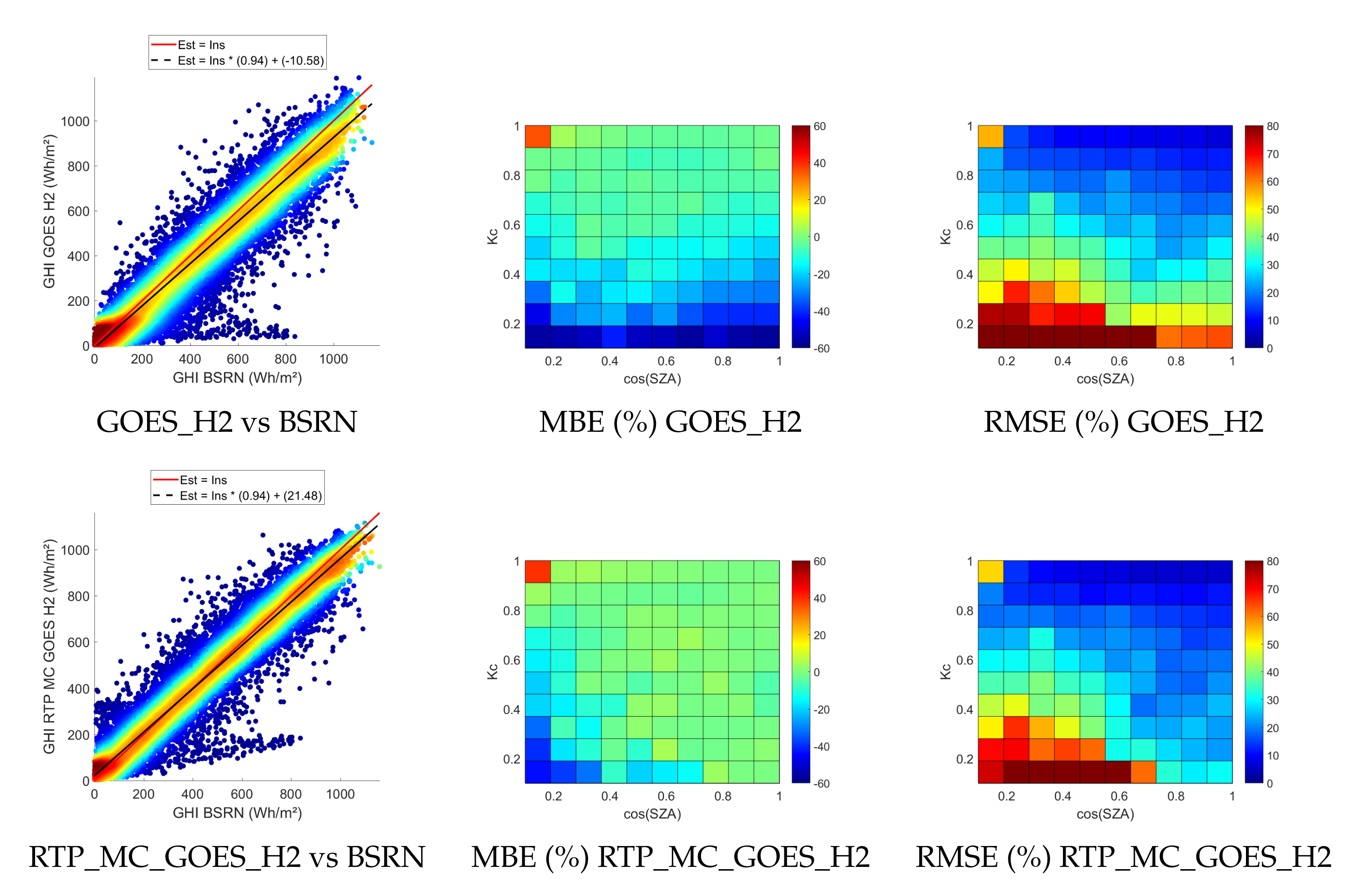
Figure 2 represents the scatter plots of the estimates versus the measured data for the overall stations as well as the mesh grids of the MBE depending on the sun zenith angle cosine and the clear-sky index K c for GOES_H2 and RTP_MC_GOES_H2. The scatter plots show that with the RTP_MC_GOES_H2 method, the line of regression is closer to the ideal case (estimates match measures) than with GOES_H2. The mesh grids show that with GOES_H2, the MBE are very low and the RMSE very high when K c is low and the cosine of the sun zenith angle is great. With, the RTP_MC_GOES_H2, these values are improved.
The MBE of the overall stations with MC_GOES_H2 ( 11.93 %) is slightly better than the one obtained with GOES_H2 ( 10.07 %) for stations located in North America. However, in South America, the MBE values obtained with MC_GOES_H2 are degraded versus those obtained with GOES_H2. Hence, the McClear clear-sky model has a low impact on the MBE, approximately 1% for North and South America.
RTP_MC_GOES_H2 significantly improves the estimates of GOES_H2 compared to MC_GOES_H2. Indeed, for the MBE, the RTP_MC_GOES_H2 provides an improvement up to ten points to the MBE while the MC_GOES_H2 improvement does not exceed three points. Regarding the RMSE, with the RTP_MC_GOES_H2, a gain up to 6 points is made while MC_GOES_H2 this value drops to 1.5 .

3.2. Comparison between GOES_H2 and RTP_MC_GOES_H2 for North America

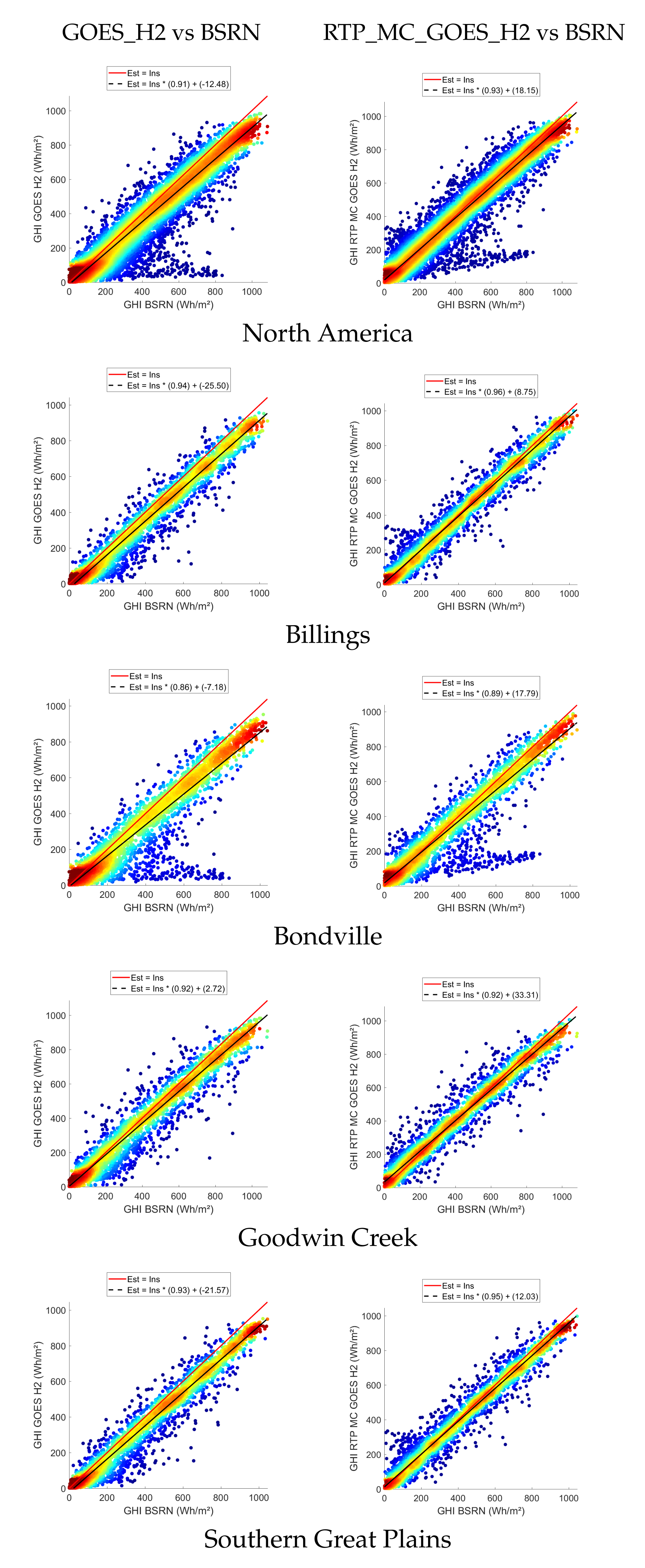
Figure 3 and Figure 4 show the scatter plots and mesh grids obtained from the analysis of North American stations.
On Figure 3, the slope of the line of regression is closer to one with RTP_MC_GOES_H2 than GOES_H2, indeed, the scatter is more compact. In addition, the color map shows that there is greater concentration of points around the ideal line.
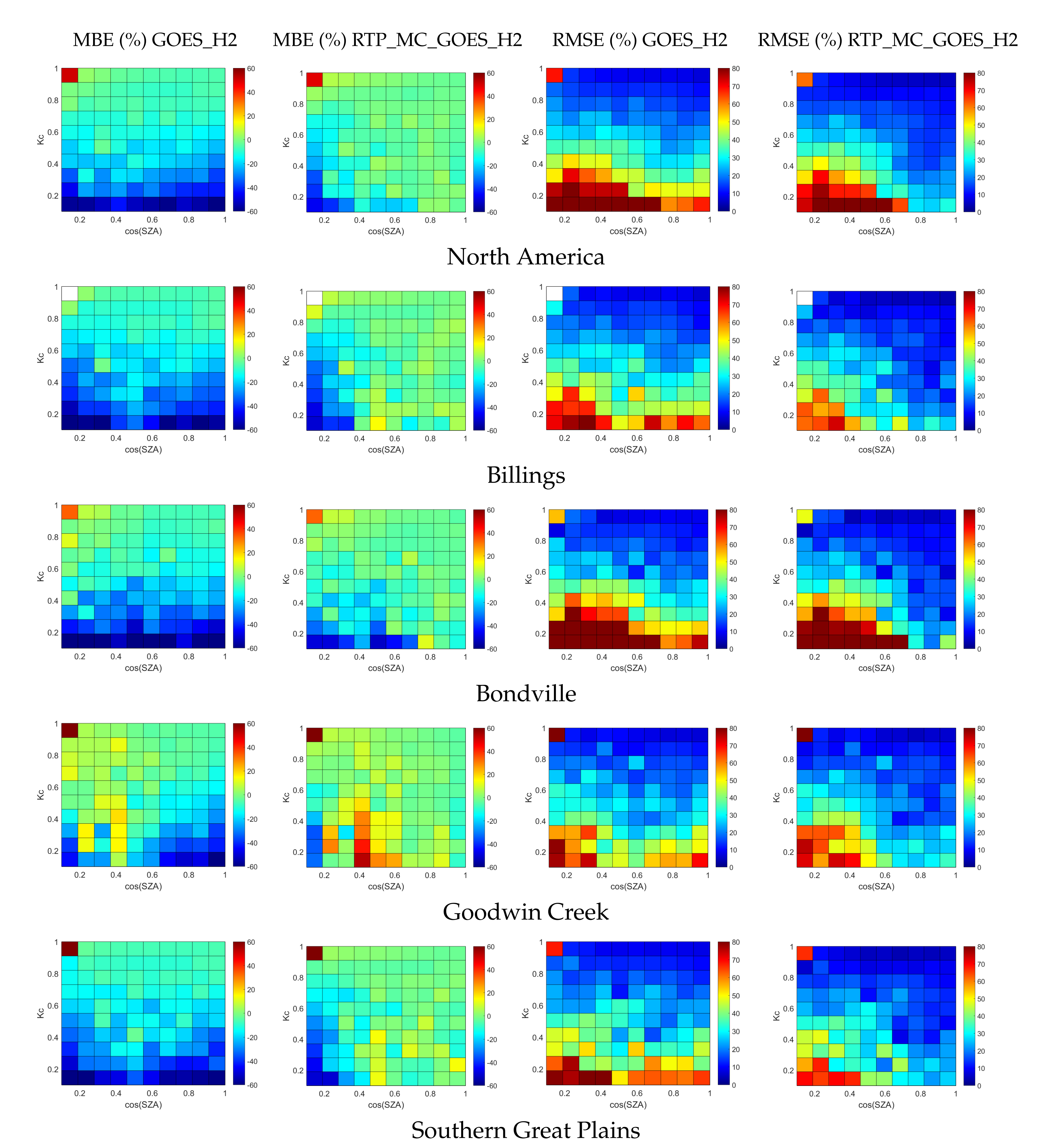
On the mesh grids on Figure 4, it can be seen that with GOES_H2 model, high (absolute) values of MBE are observed for K c < 0.6 regardless of the cosine of the sun zenith angle. Conversely, the RTP_MC_GOES_H2 gives better MBE values for all cases and even more when the cosine of the sun zenith angle is greater than 0.4 .
The RMSE mesh grids confirm that the RTP_MC_GOES_H2 gives more accurate estimates than GOES_H2. Indeed, a decrease is visible for all cases.
Next, we focus on the Bondville station, as it produced the least accurate results. Figure 5 shows the monthly RMSE against the snowfall and temperature for this station. It can be seen that the RMSE follows the snowfall evolution: the greater the snowfall, the higher the RMSE. Moreover, for January and February, the average temperature is negative; that is, snow is not only present but also remains on the ground.
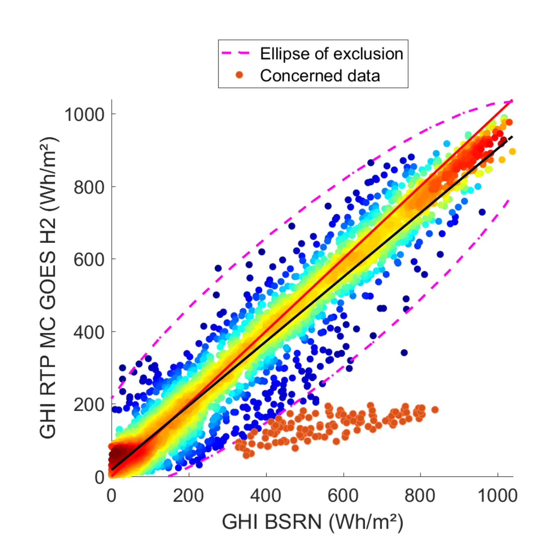
In Figure 3, the scatter plot for the Bondville station contains several points at which in situ GHI values are greater than 300 and the satellite-based estimates are below 200; that is, the model highly underestimates the surface solar irradiation. These points form a sort of spike in the scatter plot. Identifying the data in this spike can be informative. To ensure that only outliers are selected, an ellipse is defined to exclude points that may just correspond to dispersion around the regression line, as shown in Figure 6.
An analysis of this spike is summarized in Table 3. There are more than 100 data points involved, and more than half of them are observed during February, which is the month with the greatest snowfall. Almost 30 percent of the underestimated values are in March, followed by November. In fact, the months that have the greatest deviations correspond to those with a relatively large amount of snowfall. In November, only two days are of concern, and for these, the satellite images show persistent snow cover.

3.3. Comparison between GOES_H2 and RTP_MC_GOES_H2 for South America

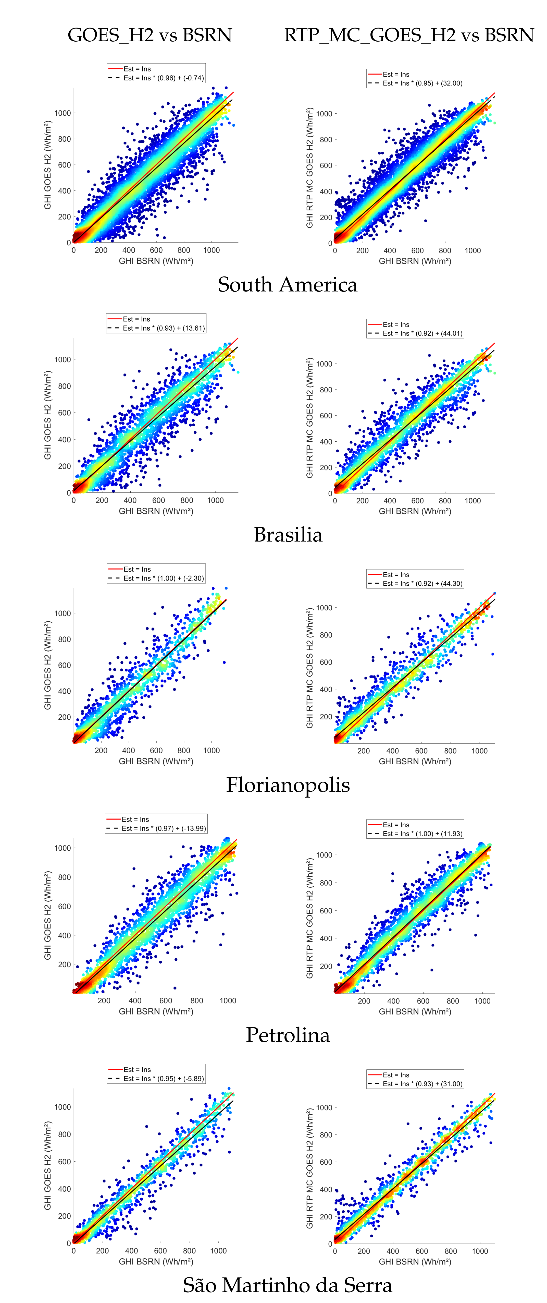
Figure 7 and Figure 8 show a comparison for stations in South America. The figures represent the scatter plots and the mesh grids of the MBE and the RMSE versus the cosine of the sun zenith angle and the clear-sky index for the GOES_H2 method and the RTP_MC_GOES_H2 one.
In Figure 7, the color map shows that there is a higher concentration of the points around the ideal regression line with the RTP_MC_GOES_H2 than with GOES_H2.
Figure 8 shows an improvement for the MBE and the RMSE. Indeed, the metrics have higher values—in absolute values for the MBE—with GOES_H2 than with RTP_MC_GOES_H2. Even if the improvement is more noticeable when the sun is high in the sky, it can be seen that the add of the RTP term improves the estimation for all skies.
The performance is poorer for the Florianopolis station. However, the coefficient of determination is very good. Figure 9 shows that the monthly RMSE increases with rainfall, which can be quite high.
In addition, the station is on an island and in front of the ocean, where sunglint effects can occur. Sunglint is the reflection of the sun on the water surface at sunrise and sunset, which can distort the data acquired by the satellite. Table 4 shows the results obtained for different periods. On the one hand, better results are obtained when omitting the 6 p.m. hour, corresponding to sunset, and the 8 a.m. hour, during which sunrise occurs. On the other hand, the minimum relative RMSE is obtained for the period from 9 a.m. to 5 p.m., but with much less data.

3.4. Comparison to Other Estimations

In this part, GOES_H2 and RTP_MC_GOES_H2 metric values are compared to those obtained with GHI estimates obtained with other methods. All data for the latter are free and provided via web services.
The following databases were used:
  • The Copernicus Atmosphere Monitoring Service (CAMS) radiation service.
    The spatial coverage is the same as that of Meteosat. Thus, GHI estimates were only compared to BSRN stations in South America. Furthermore, Meteosat has a resolution of 3 km at nadir. Moreover, Heliosat-4 is the algorithm used for the estimation [18].
  • The National Solar Radiation Database (NSRDB).
    NSRDB [41] provides GHI estimation via a physical solar model that uses information from multiple satellites. The resolution of the satellite data is about 4 km.
  • The NASA Prediction Of Worldwide Energy Resources (POWER).
    POWER [17] uses a specific NASA algorithm to estimate GHI. The method combines many types of climatic and meteorological information from different satellites. The data resolution is approximately 50 km.
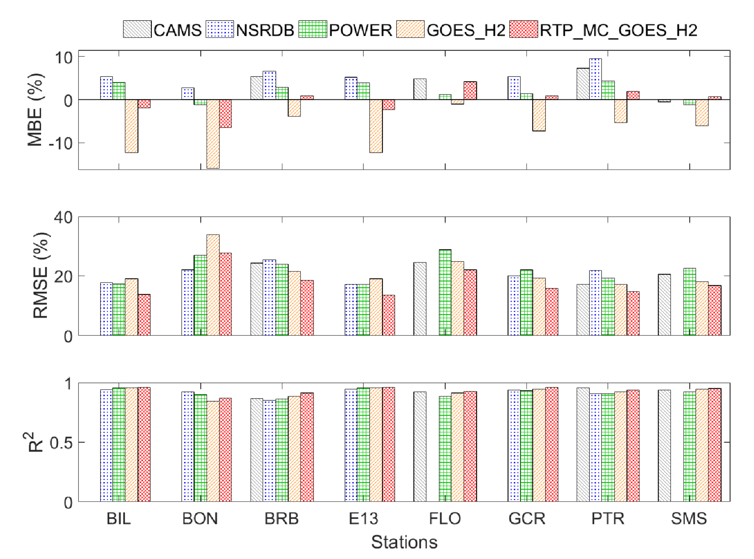
Figure 10 shows a comparison of the metrics obtained using the five datasets when considering all available data for each.
Regarding the MBE, RTP_MC_GOES_H2 provides more accurate results for all stations except Bondville and Florianopolis, while GOES_H2 estimates are the less accurate for five stations over height.
For the RMSE, the best results are obtained with RTP_MC_GOES_H2 estimates and GOES_H2 is the best second method in South America.
Following the R 2 metric, RTP_MC_GOES_H2 and CAMS give more accurate results followed closely by GOES_H2, except for Bondville.
Hence, RTP_MC_GOES_H2’s performance is better of equal to those of CAMS, NSRDB, and POWER models for all the stations but Bondville.

4. Discussion

The GOES_H2 method was updated and coupled with the McClear clear-sky model and a radiative transfer parameterization. The method was validated on eight BSRN stations located in North and South America.
RTP_MC_GOES_H2 method outperforms the original GOES_H2 method. The introduction of the radiative transfer parameterization and the McClear model shows real improvement comparing to the original method.
RTP_MC_GOES_H2 gives better results than GOES_H2 under all skies, notably when the sky is clear and the sun is high in the sky. The method is also effective, regardless of the climate type, at least for the three types encountered in this study; that is, Aw, BSh, and Cfa in the Köppen Geiger classification.
However, less accurate results were obtained for the Bondville and Florianopolis stations.
At Bondville, the RMSE results are highly correlated with the snowfall. Indeed, it is well known that snow cover negatively affects the estimation of irradiation. Snow cover reflects a high percentage of light in the visible range of the spectrum and can be considered as cloud cover in the estimation process. This situation negatively affects the estimation of the cloud index (4) and thus the surface irradiation estimation.
The discrimination between snow and cloud is generally based on the observation that, although snow and cloud are difficult to distinguish in the visible range of the spectrum, they behave differently in other ranges [42,43]. The approach would then be to combine the information of different bands of the satellite to isolate the hours where there is snow and exclude them from the computation of the cloud albedo ρ c . As theH2 method is only designed for the visible range [23], this process would be implemented in a third-party algorithm.
Two main aspects of the Florianopolis station are highlighted: the region is rainy, and it is an island. Thus, Florianopolis, as in all regions on the seafront, is affected by sunglint [44]. At sunrise and sunset, the reflection of the sun at the sea surface artificially induces a high clear-sky index value and, thus, the surface solar irradiation is overestimated.
Different methods are proposed in the literature to address sunglint effects [44]. As the best approach is to exclude data containing sunglint, many methods attempt to estimate whether sunglint will appear in a given hour. However, these estimations are frequently based on wind speed and, thus, it is necessary to be able to retrieve that information.
The metric values of the RTP_MC_GOES_H2 method estimates are better than those of CAMS, NSRDB, and POWER estimations for almost all stations: NSRDB and POWER data produce better results for the Bondville station. The meteorological and climatic data used as inputs in these models make it easier to deal with snow cover.
The RTP approach was introduced for tropical climates, but its effectiveness was demonstrated under all types of climates (encountered in the study). However, improvements can be made by first selecting the best proportionality parameter a from the radiative transfer parameter for each station individually. As the best parameter depends on the types of clouds that may be encountered in the region [28], the best a value should not be the same for all regions.
GOES-13 moved into on-orbit storage in 2018; a new satellite, GOES-16 [45], was launched in 2016 and has been in operation since 2018. Hence, to produce data estimates after 2018, it is necessary to adapt RTP_MC_GOES_H2 to GOES-16 data.

5. Conclusions

This article proposes an improvement to the GOES_H2 by updating the clear-sky model to the McClear one and introducing a radiative transfer parameterization.
The RTP_MC_GOES_H2 performs better than the GOES_H2 for surface solar irradiation estimation in North and South America.
Adding the RTP parameter improves the GHI estimates regardless of the clear-sky index value. In addition, RTP_MC_GOES_H2 gives lesser values of MBE and RMSE than the original GOES_H2 method no matter the station and the related climate (for the overall stations: 0.74 % MBE and 17.92 % for RTP_MC_GOES_H2 versus 8.91 % MBE and 21.94 % RMSE for GOES_H2). Hence, the method is effective regardless of the climate type, at least for the three types encountered in this study; that is, Aw, BSh, and Cfa in the Köppen Geiger classification. Moreover, as expected, the best estimations were obtained when the sky was clear and the sun was high in the sky.
Moreover, RTP_MC_GOES_H2 method outperforms operational CAMS, NSRDB, and POWER models for almost all stations.
Further work will focus on optimizing a method of estimating the proportionality coefficient of the radiative transfer parameter. Thus, the parameter value will adapt to different types of clouds encountered in different climates. Moreover, to enable the application of the method to more locations, establishing a means of discriminating snow from clouds is essential. In addition, addressing sunglint effects will increase the accuracy of estimations on islands, for example. These issues can be addressed by considering other bands of acquisition for the satellite or information from other satellites.
In future work, we also plan to optimize RTP_MC_GOES_H2 for the current operational satellite—GOES-16.

Author Contributions

Methodology, J.B. and T.A.; investigation, T.A. and J.B.; conceptualization, J.B. and T.A.; formal analysis, J.B. and T.A.; software, T.A. and J.B.; validation, J.B. and T.A.; resources, T.A. and J.M.; visualization, J.B.; writing, review and editing, all; supervision, S.Z., L.L. and A.P.; project administration, L.L. All authors have read and agreed to the published version of the manuscript.

Funding

This research received no external funding.

Institutional Review Board Statement

Not applicaple.

Informed Consent Statement

Not applicable.

Data Availability Statement

The satellite images are available at the Comprehensive Large-Array Stewardship System at https://www.avl.class.noaa.gov/index.html. CAMS data are available at http://www.soda-pro.com/web-services/radiation/cams-radiation-service. NSRDB data are available at https:maps.nrel.gov/nsrdb-viewer/. POWER data are available at https://power.larc.nasa.gov/data-access-viewer/, accessed on 6 December 2021.

Acknowledgments

The authors are grateful to the BSRN for supplying ground data, to NOAA for supplying satellite data via CLASS, to the SoDa website for supplying meteorological data, to the CAMS web service for supplying McClear clear-sky data and GHI estimations, and to the NSRDB for supplying GHI estimations. POWER data were obtained from the NASA Langley Research Center (LaRC) POWER Project funded through the NASA Earth Science/Applied Science Program.

Conflicts of Interest

The authors declare no conflict of interest.

References

  1. Boyle, G. Renewable Energy; Oxford University Press & The Open University: Oxford, UK, 2004. [Google Scholar]
  2. Dinçer, F. The analysis on photovoltaic electricity generation status, potential and policies of the leading countries in solar energy. Renew. Sustain. Energy Rev. 2011, 15, 713–720. [Google Scholar] [CrossRef]
  3. Program, E.S.M.A. Global Photovoltaic Power Potential by Country. 2020. Available online: https://documents1.worldbank.org/curated/en/466331592817725242/pdf/Global-Photovoltaic-Power-Potential-by-Country.pdf (accessed on 1 October 2021).
  4. Lorenz, E.; Hurka, J.; Heinemann, D.; Beyer, H.G. Irradiance Forecasting for the Power Prediction of Grid-Connected Photovoltaic Systems. IEEE J. Sel. Top. Appl. Earth Obs. Remote Sens. 2009, 2, 2–10. [Google Scholar] [CrossRef]
  5. Li, J.; Ward, J.K.; Tong, J.; Collins, L.; Platt, G. Machine learning for solar irradiance forecasting of photovoltaic system. Renew. Energy 2016, 90, 542–553. [Google Scholar] [CrossRef]
  6. Perez, R.; Seals, R.; Stewart, R.; Zelenka, A.; Estrada-Cajigal, V. Using satellite-derived insolation data for the site/time specific simulation of solar energy systems. Sol. Energy 1994, 53, 491–495. [Google Scholar] [CrossRef]
  7. Rigollier, C.; Lefèvre, M.; Wald, L. The method Heliosat-2 for deriving shortwave solar radiation from satellite images. Solar Energy 2004, 77, 159–169. [Google Scholar] [CrossRef] [Green Version]
  8. Inman, R.H.; Pedro, H.T.; Coimbra, C.F. Solar forecasting methods for renewable energy integration. Prog. Energy Combust. Sci. 2013, 39, 535–576. [Google Scholar] [CrossRef]
  9. Huang, G.; Li, Z.; Li, X.; Liang, S.; Yang, K.; Wang, D.; Zhang, Y. Estimating surface solar irradiance from satellites: Past, present, and future perspectives. Remote Sens. Environ. 2019, 233, 111371. [Google Scholar] [CrossRef]
  10. Gautier, C.; Diak, G.; Masse, S. A Simple Physical Model to Estimate Incident Solar Radiation at the Surface from GOES Satellite Data. J. Appl. Meteorol. Climatol. 1980, 19, 1005–1012. [Google Scholar] [CrossRef] [Green Version]
  11. O’Hirok, W.; Gautier, C. A Three-Dimensional Radiative Transfer Model to Investigate the Solar Radiation within a Cloudy Atmosphere. Part I: Spatial Effects. J. Atmos. Sci. 1998, 55, 2162–2179. [Google Scholar] [CrossRef]
  12. Perez, R.; Ineichen, P.; Moore, K.; Kmiecik, M.; Chain, C.; George, R.; Vignola, F. A New Operational Model for Satellite-Derived Irradiances: Description and Validation. Solar Energy 2002, 73, 307–317. [Google Scholar] [CrossRef] [Green Version]
  13. Martins, F.; Pereira, E.; Abreu, S. Satellite-derived solar resource maps for Brazil under SWERA project. Sol. Energy 2007, 81, 517–528. [Google Scholar] [CrossRef]
  14. Stephens, G.L.; Gabriel, P.M.; Partain, P.T. Parameterization of Atmospheric Radiative Transfer. Part I: Validity of Simple Models. J. Atmos. Sci. 2001, 58, 3391–3409. [Google Scholar] [CrossRef]
  15. Sengupta, M.; Habte, A.; Gueymard, C.; Wilbert, S.; Renne, D. Best Practices Handbook for the Collection and Use of Solar Resource Data for Solar Energy Applications, 2nd ed.; National Renewable Energy Laboratory: Golden, CO, USA, 2017. [Google Scholar] [CrossRef]
  16. Gueymard, C.A. REST2: High-performance solar radiation model for cloudless-sky irradiance, illuminance, and photosynthetically active radiation—Validation with a benchmark dataset. Sol. Energy 2008, 82, 272–285. [Google Scholar] [CrossRef]
  17. Sparks, A.H. nasapower: A NASA POWER Global Meteorology, Surface Solar Energy and Climatology Data Client for R. J. Open Source Softw. 2018, 3, 1035. [Google Scholar] [CrossRef] [Green Version]
  18. Qu, Z.; Oumbe, A.; Blanc, P.; Espinar, B.; Gesell, G.; Gschwind, B.; Klüser, L.; Lefèvre, M.; Saboret, L.; Schroedter-Homscheidt, M.; et al. Fast radiative transfer parameterisation for assessing the surface solar irradiance: The Heliosat-4 method. Meteorol. Z. 2017, 26, 33–57. [Google Scholar] [CrossRef]
  19. Lefèvre, M.; Oumbe, A.; Blanc, P.; Espinar, B.; Gschwind, B.; Qu, Z.; Wald, L.; Schroedter-Homscheidt, M.; Hoyer-Klick, C.; Arola, A.; et al. McClear: A new model estimating downwelling solar radiation at ground level in clear-sky conditions. Atmos. Meas. Tech. 2013, 6, 2403–2418. [Google Scholar] [CrossRef] [Green Version]
  20. Oumbe, A.; Qu, Z.; Blanc, P.; Lefèvre, M.; Wald, L.; Cros, S. Decoupling the effects of clear atmosphere and clouds to simplify calculations of the broadband solar irradiance at ground level. Geosci. Model Dev. 2014, 7, 1661–1669. [Google Scholar] [CrossRef] [Green Version]
  21. Betcke, J.; Kuhlemann, R.; Hammer, A.; Drews, A.; Lorenz, E.; Girodo, M.; Heinemann, D.; Wald, L.; Cros, S.; Schroedter-Homscheidt, M.; et al. Energy-Specific Solar Radiation Data from Meteosat Second Generation (MSG): The Heliosat-3 Project, Final Report; Technical Report; University of Oldenburg: Oldenburg, Germany, 2006. [Google Scholar] [CrossRef]
  22. Mueller, R.; Dagestad, K.; Ineichen, P.; Schroedter-Homscheidt, M.; Cros, S.; Dumortier, D.; Kuhlemann, R.; Olseth, J.; Piernavieja, G.; Reise, C.; et al. Rethinking satellite-based solar irradiance modelling: The SOLIS clear-sky module. Remote Sens. Environ. 2004, 91, 160–174. [Google Scholar] [CrossRef]
  23. Rigollier, C.; Bauer, O.; Wald, L. On the clear sky model of the ESRA—European Solar Radiation Atlas—With respect to the heliosat method. Sol. Energy 2000, 68, 33–48. [Google Scholar] [CrossRef] [Green Version]
  24. Albarelo, T.; Marie-Joseph, I.; Primerose, A.; Seyler, F.; Wald, L.; Linguet, L. Optimizing the Heliosat-II Method for Surface Solar Irradiation Estimation with GOES Images. Can. J. Remote. Sens. 2015, 41, 86–100. [Google Scholar] [CrossRef]
  25. Lefèvre, M.; Wald, L.; Diabate, L. Using reduced data sets ISCCP-B2 from the Meteosat satellites to assess surface solar irradiance. Solar Energy 2007, 81, 240–253. [Google Scholar] [CrossRef] [Green Version]
  26. Marie-Joseph, I.; Linguet, L.; Gobindass, M.L.; Wald, L. On the applicability of the Heliosat-2 method to assess surface solar irradiance in the intertropical convergence zone, French Guiana. Int. J. Remote Sens. 2013, 34, 3012–3027. [Google Scholar] [CrossRef] [Green Version]
  27. Fillol, E.; Albarelo, T.; Primerose, A.; Wald, L.; Linguet, L. Spatiotemporal indicators of solar energy potential in the Guiana Shield using GOES images. Renew. Energy 2017, 111, 11–25. [Google Scholar] [CrossRef] [Green Version]
  28. Diallo, M.; Albarelo, T.; Primerose, A.; Linguet, L. Improving the Heliosat-2 method for surface solar irradiation estimation under cloudy sky areas. Solar Energy 2018, 169, 565–576. [Google Scholar]
  29. McArthur, L.J.B. Baseline Surface Radiation Network (BSRN). Operations Manual. 2005. Available online: https://bsrn.awi.de/ (accessed on 1 June 2018).
  30. National Aeronautics and Space Administration. GOES N Data Book. 2005. Available online: https://www.nasa.gov/pdf/148080main_GOES-N%20Databook%20with%20Copyright.pdf (accessed on 1 October 2021).
  31. Nguyen, L.; Doelling, D.; Minnis, P.; Ayers, J.K. Rapid technique to cross-calibrate satellite imager visible channels. In Proceedings of the SPIE Proceedings, Denver, CO, USA, 26 October 2004; Volume 5542. [Google Scholar] [CrossRef]
  32. Taylor, V.R.; Stowe, L.L. Reflectance characteristics of uniform Earth and cloud surfaces derived from NIMBUS-7 ERB. J. Geophys. Res. Atmos. 1984, 89, 4987–4996. [Google Scholar] [CrossRef]
  33. Remund, J.; Wald, L.; Lefèvre, M.; Ranchin, T.; Page, J. Worldwide Linke Turbidity Information. In Proceedings of the ISES Solar World Congress, Goteborg, Sweden, 16–19 June 2003. [Google Scholar]
  34. CAMS McClear Service for Irradiation under Clear-Sky. Available online: http://www.soda-pro.com/web-services/radiation/cams-mcclear (accessed on 1 October 2021).
  35. Gautier, C.; Landsfeld, M. Surface Solar Radiation Flux and Cloud Radiative Forcing for the Atmospheric Radiation Measurement (ARM) Southern Great Plains (SGP): A Satellite, Surface Observations, and Radiative Transfer Model Study. J. Atmos. Sci. 1997, 54, 1289–1307. [Google Scholar] [CrossRef]
  36. Diak, G.; Gautier, C. Improvements to a Simple Physical Model for Estimating Insolation From GOES Data. J. Appl. Meteorol. 1983, 22, 505–508. [Google Scholar] [CrossRef] [Green Version]
  37. Geiger, M.; Diabaté, L.; Ménard, L.; Wald, L. A web service for controlling the quality of measurements of global solar irradiation. Sol. Energy 2002, 73, 475–480. [Google Scholar] [CrossRef] [Green Version]
  38. Kottek, M.; Grieser, J.; Beck, C.; Rudolf, B.; Rubel, F. World Map of the Köppen-Geiger climate classification updated. Meteorol. Z. 2006, 15, 259–263. [Google Scholar] [CrossRef]
  39. Global Modeling and Assimilation Office (GMAO). MERRA-2 tavg1_2d_slv_Nx: 2d,1-Hourly, Time-Averaged, Single-Level, Assimilation, Single-Level Diagnostics V5.12.4, Greenbelt, MD, USA, Goddard Earth Sciences Data and Information Services Center (GES DISC). 2015. Available online: https://cmr.earthdata.nasa.gov/search/concepts/C1276812862-GES_DISC.html (accessed on 5 May 2021). [CrossRef]
  40. Gelaro, R.; McCarty, W.; Suárez, M.J.; Todling, R.; Molod, A.; Takacs, L.; Randles, C.A.; Darmenov, A.; Bosilovich, M.G.; Reichle, R.; et al. The Modern-Era Retrospective Analysis for Research and Applications, Version 2 (MERRA-2). J. Clim. 2017, 30, 5419–5454. [Google Scholar] [CrossRef]
  41. Sengupta, M.; Xie, Y.; Lopez, A.; Habte, A.; Maclaurin, G.; Shelby, J. The National Solar Radiation Data Base (NSRDB). Renew. Sustain. Energy Rev. 2018, 89, 51–60. [Google Scholar] [CrossRef]
  42. Allen, R.C.; Durkee, P.A.; Wash, C.H. Snow/Cloud Discrimination with Multispectral Satellite Measurements. J. Appl. Meteorol. Climatol. 1990, 29, 994–1004. [Google Scholar] [CrossRef] [Green Version]
  43. Miller, S.D.; Lee, T.F.; Fennimore, R.L. Satellite-Based Imagery Techniques for Daytime Cloud/Snow Delineation from MODIS. J. Appl. Meteorol. 2005, 44, 987–997. [Google Scholar] [CrossRef]
  44. Kay, S.; Hedley, J.D.; Lavender, S. Sun Glint Correction of High and Low Spatial Resolution Images of Aquatic Scenes: A Review of Methods for Visible and Near-Infrared Wavelengths. Remote Sens. 2009, 1, 697–730. [Google Scholar] [CrossRef] [Green Version]
  45. Schmit, T.J.; Griffith, P.; Gunshor, M.M.; Daniels, J.M.; Goodman, S.J.; Lebair, W.J. A Closer Look at the ABI on the GOES-R Series. Bull. Am. Meteorol. Soc. 2017, 98, 681–698. [Google Scholar] [CrossRef]
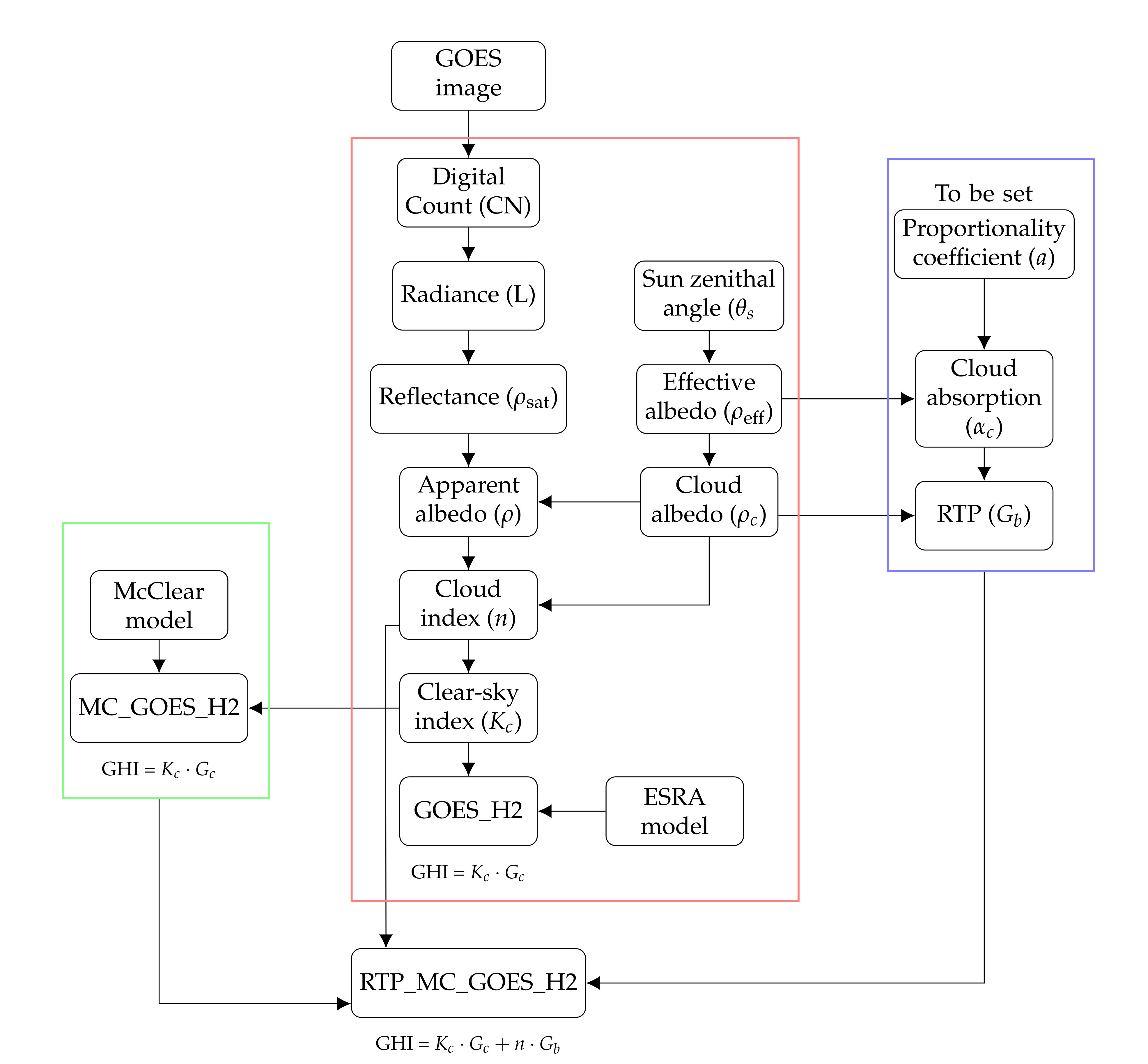
Figure 1. Flowchart of the methods. GOES_H2 method is in the red block, in the green block is the MC_GOES_H2 method and blue block illustrates the radiative transfer parameterization.
Remotesensing 14 00224 g001
Figure 2. Comparison between hourly GHI estimates using the GOES_H2 and RTP_MC_GOES_H2 methods and BSRN data for all stations together. The scatters on first column represent the GHI estimates using GOES_H2 (top) and RTP_MC_GOES_H2 (down) versus the measured values; the black line corresponds to the ideal case, where estimates match measurements, and the red line shows the results of linear regression. In the color map (ranging from blue to red), the warmer the color, the higher the concentration of points. Second and third columns are mesh grids of the MBE (%) and RMSE (%), respectively, as a function of the clear-sky index and the cosine of the solar zenith angle of the estimates obtained with GOES_H2 (top) and RTP_MC_GOES_H2 (down) method.
Remotesensing 14 00224 g002
Figure 3. Comparison between hourly GHI estimates using the GOES_H2 (first column) and RTP_MC_GOES_H2 (second column) methods and BSRN data for stations in North America. The black line corresponds to the ideal case, where estimates match measurements, and the red line represents the results of linear regression. In the color map (ranging from blue to red), the warmer the color, the higher the concentration of points.
Remotesensing 14 00224 g003
Figure 4. Comparison between hourly GHI estimates using the GOES_H2 and the RTP_MC_GOES_H2 models and BSRN data for stations in North America. The first and third columns are mesh grids of the MBE (%) and RMSE (%), respectively, as a function of the clear-sky index and the cosine of the solar zenith angle for GOES_H2 model and second and fourth columns represent the same but for RTP_MC_GOES_H2 model.
Remotesensing 14 00224 g004
Figure 5. Representation of (a) the monthly RMSE and snowfall and (b) average temperature for the Bondville station.
Remotesensing 14 00224 g005
Figure 6. Representation of the data considered for studying the spike for the Bondville station.
Remotesensing 14 00224 g006
Figure 7. Comparison between hourly GHI estimates using the GOES_H2 (first column) and RTP_MC_GOES_H2 (second column) methods and BSRN data for stations in South America. The black line corresponds to the ideal case, where estimates match measurements, and the red line represents the results of linear regression. In the color map (ranging from blue to red), the warmer the color, the higher the concentration of points.
Remotesensing 14 00224 g007
Figure 8. Comparison between hourly GHI estimates using the GOES_H2 and the RTP_MC_GOES_H2 models and BSRN data for stations in South America. The first and third columns are mesh grids of the MBE (%) and RMSE (%), respectively, as a function of the clear-sky index and the cosine of the solar zenith angle for GOES_H2 model and the second and fourth columns represent the same but for RTP_MC_GOES_H2 model.
Remotesensing 14 00224 g008
Figure 9. Representation of the monthly rainfall and the monthly RMSE for the Florianopolis station.
Remotesensing 14 00224 g009
Figure 10. Comparison of GHIestimates from GOES_H2 and RTP_MC_GOES_H2 to other methods. The stations name abbreviations correspond to: Billings (BIL), Bondville (BON), Brasilia (BRB), Southern Great Plains (E13), Florianopolis (FLO), Goodwin Creek (GCR), Petrolina (PTR), and São Martinho da Serra (SMS).
Remotesensing 14 00224 g010
Table 1. Chosen BSRN stations.
StationLocationLatitudeLongitudeAltitude (m)
North America
BillingsCenter 36.605 ° N 97.485 ° W317
BondvilleCenter/East 40.067 ° N 88.367 ° W213
Goodwin CreekCenter/East 34.255 ° N 89.873 ° W98
Southern Great PlainsCenter 36.605 ° N 97.485 ° W318
South America
BrasiliaCenter 15.601 ° S 47.713 ° W1023
FlorianopolisSouth 27.605 ° S 48.523 ° W11
PetrolinaCenter/North 9.068 ° S 40.319 ° W387
São Martinho da SerraSouth 29.443 ° S 53.823 ° W489
Table 2. Comparison between hourly GHI estimation using GOES_H2, MC_GOES_H2 and RTP_MC_GOES_H2 and BSRN data.
Number of Data and Mean of Global Horizontal Irradiation
StationNumber of DataGHI Mean Wh/m 2
BSRNGOES_H2MC_GOES_H2RTP_MC_GOES_H2
All24,423 408.59 372.19 375.36 405.57
North America15,614 384.09 338.26 345.42 374.8
Billings3832 401.72 352.11 365.5 393.73
Bondville3953 360.3 302.57 305.84 336.94
Goodwin Creek3995 373.2 346.24 346.69 376.5
Southern Great Plains 3 834 402.34 352.9 364.81 393.12
South America8809 452.01 432.34 428.44 460.11
Brasilia2874 474.08 455.52 446.85 478.74
Florianopolis1522 355.43 351.84 330.42 370.47
Petrolina3050 503.45 476.7 486.03 513.61
São Martinho da Serra1363 398.23 374.11 370.24 401.2
Mean Bias Error
Station MBE Wh/m 2 (%)
GOES_H2MC_GOES_H2RTP_MC_GOES_H2
All 36.39 ( 8.91 ) 33.22 ( 8.13 ) 3.02 ( 0.74 )
North America 45.83 ( 11.93 ) 38.67 ( 10.07 ) 9.29 ( 2.42 )
Billings 49.6 ( 12.35 ) 36.21 ( 9.01 ) 7.98 ( 1.99 )
Bondville 57.72 ( 16.02 ) 54.45 ( 15.11 ) 23.35 ( 6.48 )
Goodwin Creek 26.96 ( 7.22 ) 26.5 ( 7.1 ) 3.3 ( 0.88 )
Southern Great Plains 49.44 ( 12.29 ) 37.53 ( 9.33 ) 9.22 ( 2.29 )
South America 19.67 ( 4.35 ) 23.57 ( 5.21 ) 8.1 ( 1.79 )
Brasilia 18.56 ( 3.91 ) 27.23 ( 5.74 ) 4.66 ( 0.98 )
Florianopolis 3.6 ( 1.01 ) 25.02 ( 7.04 ) 15.03 ( 4.23 )
Petrolina 26.75 ( 5.31 ) 17.42 ( 3.46 ) 10.16 ( 2.02 )
São Martinho da Serra 24.11 ( 6.05 ) 27.99 ( 7.03 ) 2.97 ( 0.75 )
Root-Mean Square Error
Station RMSE Wh/m 2 (%)
GOES_H2MC_GOES_H2RTP_MC_GOES_H2
All 86.63 ( 21.94 ) 87.08 ( 21.31 ) 73.22 ( 17.92 )
North America 89.26 ( 23.24 ) 86.27 ( 22.46 ) 70.05 ( 18.24 )
Billings 76.69 ( 19.09 ) 70.52 ( 17.55 ) 55.31 ( 13.77 )
Bondville 121.84 ( 33.82 ) 120.33 ( 33.4 ) 99.71 ( 27.67 )
Goodwin Creek 71.8 ( 19.24 ) 72.03 ( 19.3 ) 59.31 ( 15.89 )
Southern Great Plains 76.77 ( 19.08 ) 70.73 ( 17.58 ) 54.89 ( 13.64 )
South America 90.29 ( 19.97 ) 88.5 ( 19.58 ) 78.51 ( 17.37 )
Brasilia 102.13 ( 21.54 ) 101.4 ( 21.39 ) 87.93 ( 18.54 )
Florianopolis 88.49 ( 24.89 ) 87.69 ( 24.67 ) 78.56 ( 22.1 )
Petrolina 86.5 ( 17.18 ) 81.66 ( 16.22 ) 73.83 ( 14.66 )
São Martinho da Serra 72.13 ( 18.11 ) 73.73 ( 18.51 ) 66.64 ( 16.73 )
Table 3. Analysis of data forming the spike in the Bondville scatter plot.
MonthNumber of Data% of Data Involved
15 4.2
268 57.14
337 31.09
81 0.8
118 6.72
Table 4. Comparison of results for the Florianopolis station with different time considerations.
ConfigurationNumber of DataMBE Wh/m 2 (%)RMSE Wh/m 2 (%)R 2
8–18 h1522 15.04 ( 4.23 ) 78.56 ( 22.1 ) 0.93
9–17 h1175 17.62 ( 4.13 ) 86.18 ( 20.2 ) 0.91
Publisher’s Note: MDPI stays neutral with regard to jurisdictional claims in published maps and institutional affiliations.