An Enhanced Data-Driven Array Shape Estimation Method Using Passive Underwater Acoustic Data

Abstract

Beamforming-based signal enhancement technologies in passive sonar array processing often have poor performance due to array distortion caused by rapid tactical maneuvers of the towed platform, oceanic currents, hydrodynamic effects, etc. In this paper, an enhanced data-driven shape array estimation formulation is proposed using passive underwater acoustic data. Beamforming based on a hypothetically ideal array is firstly employed to perform the detection of narrow-band components from sources of opportunity, and the corresponding phases of these detected narrow-band components are subsequently extracted to acquire time-delay differences. Then, a weighted outlier-robust Kalman smoother is proposed to acquire enhanced estimates of the time-delay differences, since the underlying properties of slowly changing time-delay differences in the hydrophone array and diverse signal to interference and noise ratios in multiple narrow-band components are explored; and its Cramer–Rao Lower Bound is also provided. Finally, the hydrophone array shape is estimated based on the estimated time delay differences. The proposed formulation fully exploits directional radiated noise signals from distant underwater acoustic targets as sources of opportunity for real-time array shape estimation, and thus it requires neither the number nor direction of sources to be known in advance. The effectiveness of the proposed method is validated in simulations and real experimental data.

1. Introduction

Hydrophone arrays are widely used in underwater acoustics to perform direction-of-arrival (DOA) estimation and beamforming-based signal enhancement in the passive sonar system. Most array signal processing techniques are based on the assumption that the shape of the array remains unchanged. Unfortunately, the shape of a hydrophone array, such as a towed array, is often perturbed due to fluctuations in ship tactical maneuvering, oceanic currents, nonneutral buoyancy, and so on, particularly in the demand of the long-towed arrays for the acquisition of a low-frequency signal source at long range. These would lead to uncertainty in array shape and deviation from the hypothetical one [1,2,3,4]. However, beamforming as a typical signal enhancement technique requires knowledge of accurate array positions to properly process the measurements, which means an accurate estimate of the array shape is required to properly beamform the acoustic arrivals. The uncertainty in array shape inevitably degrades the beamforming performance [2]. A theoretical derivation of the performance loss in a distorted array shape due to the tactical maneuvering is provided [5]. Therefore, it is requisite to implement an array shape estimation to improve the acoustic system performance.

1.1. Related Works

A huge amount of effort has been devoted to array shape estimation. In general, these methods can be classified into source-independent methods and source-dependent methods. For source-independent methods, one effective method is to place depth-measurement sensors and compasses at several points within the array. These additional sensors provide localized respectively vertical and horizontal information on the transverse displacements of the array, whereas it is less economical due to the use of additional sensors. Further work is to model the array shape by a low order polynomial and to use the available sensors’ information to determine the coefficients of this polynomial [6]. A Kalman filter technique with a small angle approximation is used to estimate the array shape evolution over time [7], and an extended Kalman filter approach is also considered with the predicted state update following a higher-order nonlinear model [8].

As for source-dependent methods, acoustic hydrophone data would be used to estimate the array shape when there is no sensors’ information within the array or there are too few working sensors, and the shape can be estimated by measuring the relative time or phase delays among sensors due to one or more sources with known or unknown directions [9,10,11,12,13,14,15,16,17,18,19]. Historically, the array shape model employed for acoustic-based estimation is often considered to be a horizontal axis with perturbations at regular intervals on the vertical axis. Under this formulation, the Cramer–Rao Lower Bound (CRLB) for the narrow-band plane-wave sources is provided for source localization with a single known source direction or a known angle between the first receiver and the second one [9]. The maximum-likelihood (ML) approach is used to jointly estimate both the array and source parameters for multiple narrow-band or broadband sources with the known number of sources through a two-stage iteration procedure [10]. Subspace-based eigenvector techniques form another way to estimate array shapes when a single source at a known frequency and direction is known [11]. The eigenvector method for estimating the positions of the array elements is based on the eigen-decomposition of the array covariance matrix to acquire the phase delays between adjacent array elements. The statistic of phase delays is analyzed in [12]. The CRLB of the subspace-based array shape estimation method is provided in [3]. The eigenvector method is similar to the method [13], and it can be also regarded as a special case of the maximum-likelihood method [14]. Reference [15] proposes an improved array shape estimation method by jointly exploiting the acoustic hydrophone data and sensor data.

1.2. Contributions

In this paper, an enhanced data-driven array shape estimation formulation is proposed using passive underwater acoustic data. Instead of using the traditional method with a deterministic signal model and a known number of discrete sources, a novel data-driven approach is proposed by exploiting these directionals radiated noise sources, such as shipping and cargo as sources of opportunity for real-time array shape estimation. The conventional beamforming based on the hypothetical uniform linear array is firstly employed to acquire an improved waveform due to spatial gain from the hydrophone array. Since the radiated noise sources involve the amount of narrow-band components that originated from the vibration of mechanical components like diesel generator and air conditioning equipment, we perform the narrow-band frequency detection and extract their corresponding phases for the acquisition of noisy time-delay differences. A novel weighted outlier-robust Kalman smoother (WORKS) method is then proposed to acquire enhanced time-delay estimates by exploring the properties of slowly changing time-delay difference in hydrophone array as well as the diverse signal to interference and noise ratios (SINR) in multiple narrow-band components, and its CRLB is also analyzed and provided. Finally, the hydrophone array shape is obtained using the estimated time delay differences, and thus beamforming-based improved radiated noise signal is acquired. The proposed formulation fully exploits the directional radiated noise source signals as sources of opportunity for real-time array shape estimation, and thus it requires neither the number nor direction of sources to be known in advance. Furthermore, the proposed WORKS approach has the capability of acquiring the enhanced time-delay difference estimation by treating the weights associated with each observed noisy time-delay difference data in a probabilistic approach.

The contributions of the paper lie in three aspects: (1) An enhanced data-driven array shape estimation formulation using passive underwater acoustic data is provided. The proposed formulation fully exploits the directional radiated noise source signals as sources of opportunity for real-time array shape estimation, and thus it requires neither the number nor direction of sources to be known in advance. (2) A novel weighted outlier-robust Kalman smoother method is proposed to acquire enhanced time-delay estimates by the exploitation of slowly changing time-delay differences in hydrophone array and has the capability of alleviating the effects of the outliers resulted from the diverse noise levels in the multiple frequencies. (3) The CRLB of the proposed method is analyzed.

1.3. Organization and Notation

The paper is organized as follows: The underwater acoustic radiated noise signal model is introduced in Section 2. A novel array shape estimate technique is described in Section 3, and the weighted robust-outlier Kalman smoother method is also proposed in this section. Performance bound is also provided in Section 3. Simulations and experiments demonstrate the robustness of the proposed algorithms compared to conventional methods in Section 4. Concluding remarks are given in Section 5.

Notation: We use lower-case (upper-case) bold characters to denote vectors (matrices). $p(·)$ denotes the probability density function (pdf), and $\mathcal{N}\left(x\right|a,b)$ denotes that random variable x follows a Gaussian distribution with mean a and variance b. In addition, ${(·)}^T$ and ${(·)}^H$ denote transpose and conjugate transpose, respectively, ${\mathbf{I}}_N$ denotes the $N\times N$ identity matrix. ${\nabla }_{\mathbf{x}}=\left[\frac{\partial }{\partial x_1},\cdots ,\frac{\partial }{\partial x_N}\right]$ denotes the gradient operator respect to the variable vector $\mathbf{x}={\left[x_1,\cdots ,x_N\right]}^T\in {\mathcal{R}}^{N\times 1}$, and $\mathbb{E}\left(x\right)$ represents the expectation operator of the random variable x.

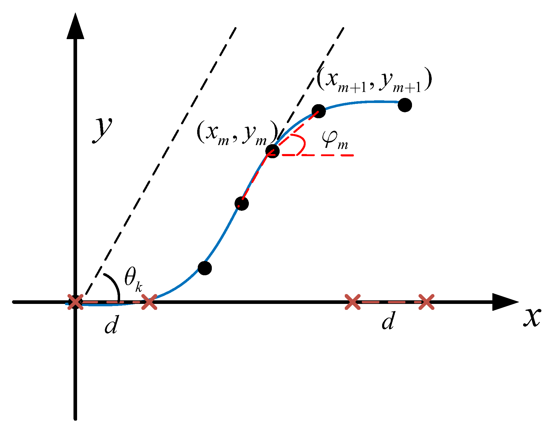
2. Underwater Acoustic Radiated Noise Model in the Distorted Array

In this section, the underwater acoustic radiated noise model in a distorted hydrophone array is introduced. We assume that a thin flexible cable with M omnidirectional hydrophone sensors mounted at fixed inter-element spacing d is employed. Due to the transverse motion of ship tactical maneuvering, oceanic currents, and hydrodynamic effects, it would result in transverse displacements of the array from a straight line, as shown in Figure 1. The positions of the first two sensors define a baseline for the coordinate system and consequently are always assumed to reside on the x axis. It is observed that a deformed array occurs when any one of the inner sensor y positions are no longer zero.

The deformation is caused by bending at the sensor junctions due to the soft and elastic external shell of hydrophone array, which implies that the inter-sensor distances remain constant, and thus we have,

$$\begin{array}{c}\hfill d=\sqrt{{(x_{m+1}-x_m)}^2+{(y_{m+1}-y_m)}^2},m=0,\cdots ,M-1,\end{array}$$

(1)

where the location of the mth sensor is denoted by $(x_m,y_m)$ in the $x-y$ Cartesian plane.

With respect to K far-field sources of opportunity impinging on the hydrophone array and the source with the bearing or direction of ${\theta }_k$, the range difference between the first two sensors becomes, as shown in Figure 1,

$$\begin{array}{c}\hfill \Delta r_{k,0}=r_{k,1}-r_{k,0}\approx dcos{\theta }_k=\left(x_1-x_0\right)cos{\theta }_k,\end{array}$$

(2)

where $r_{k,1}$ and $r_{k,0}$ denote the distances from the kth source to the second and reference sensors, respectively, and the result above is based on the far-field hypothesis. However, the locations of sensors deviate from the nominal ones, when the hydrophone array shape is distorted or deformed. Assuming the deviation angle formed by the line between the mth sensor and $(m+1)$th sensor along x axis is denoted as ${\varphi }_m$, the range difference becomes,

$$\begin{array}{c}\hfill \Delta r_{k,m}\approx dcos({\theta }_k-{\varphi }_m)=\left(x_{m+1}-x_m\right)cos{\theta }_k+\left(y_{m+1}-y_m\right)sin{\theta }_k.\end{array}$$

(3)

For the first two sensors as a baseline, ${\varphi }_0=0$. The range difference between the mth sensor and the reference can be written by,

$$\begin{array}{c}\hfill r_{k,m}-r_{k,0}=\sum _{i=0}^{m-1}\Delta r_{k,i}=\sum _{i=0}^{m-1}dcos({\theta }_k-{\varphi }_i)=\sum _{i=0}^{m-1}\left(x_{i+1}-x_i\right)cos{\theta }_k+\left(y_{i+1}-y_i\right)sin{\theta }_k.\end{array}$$

(4)

The corresponding time-delay difference is

$$\begin{array}{c}\hfill {\tau }_{k,m}=\frac{{\sum }_{i=0}^{m-1}\Delta r_{k,i}}{v}=\sum _{i=0}^{m-1}\Delta {\tau }_{k,i},\end{array}$$

(5)

where v is the speed of acoustic wave in water, and $\Delta {\tau }_{k,i}$ denotes the time-delay difference between the $(i+1)$th and ith sensors with respect to the source of opportunity. It should be noted that the accuracies of the array shape estimates will be confined to the accuracies of each estimated time-delay difference for adjacent sensors, giving rise to error accumulations of the time-delay difference according to Equation (5).

Assuming the kth radiated noise source signal as $s_k\left(t\right)$ with the bearing of ${\theta }_k$, the received signal $y_m\left(t\right)$ in the mth sensor can be written as

$$\begin{array}{c}\hfill y_m\left(t\right)=\sum _{k=1}^K{\zeta }_{k,m}{s}_k\left(t-{\tau }_{k,m}\right)+e_m\left(t\right),\end{array}$$

(6)

where ${\zeta }_{k,m}$ and ${\tau }_{k,m}$, represent respectively the amplitude and time delay from the source to the mth sensor, and $e_m\left(t\right)$ is an additive noise.

According to the statistical model of the underwater acoustic radiated noise [20,21], the corresponding time-domain $s_k\left(t\right)$ is expressed by,

$$\begin{array}{c}\hfill s_k\left(t\right)=p_{kl}\left(t\right)+\left(1+p_{km}\left(t\right)\right)p_{kc}\left(t\right),\end{array}$$

(7)

where $p_{kl}\left(t\right)$ is a narrow-band signal arised from the vibration of machinery, $p_{km}\left(t\right)$ represents a modulation function due to the propeller movement, and $p_{kc}\left(t\right)$ denotes a stationary hydrodynamic noise.

The narrow-band signal $p_{kl}\left(t\right)$, which is often generated from the vibration of mechanical components like diesel generator and air conditioning equipment, can be denoted by the superposition of multiple sinusoid signals as,

$$\begin{array}{c}\hfill p_{kl}\left(t\right)=\sum _{l=1}^L{\alpha }_{kl}sin\left(2\pi f_{kl}t\right),\end{array}$$

(8)

where ${\alpha }_{kl}$ is an amplitude of the lth single-tone frequency from the source, L is the number of the sinusoid signals, and $f_{kl}$ is the corresponding frequency.

In the real sonar system, the narrow-band signals in the underwater acoustic radiation noise often have high source levels owing to inevitable mechanical vibration, and thus they are easier to be detected and recognized, compared to the broadband hydrodynamic noise signals [20,21]. Figure 2 shows a typical spectrum example of radiated noise from a ship. It is observed that there exist several narrow-band frequencies that have higher powers and are prominent in their nearby frequency ranges, their phases involve the information of time delays between the sources of opportunity and sensors in the deformed array. It possibly provides a way to estimate the distorted array shape.

3. Array Shape Estimation

In this section, a novel data-driven array shape estimation formulation will be provided, and the weighted robust-outlier Kalman smoother method is proposed to acquire an enhanced time-delay difference estimation.

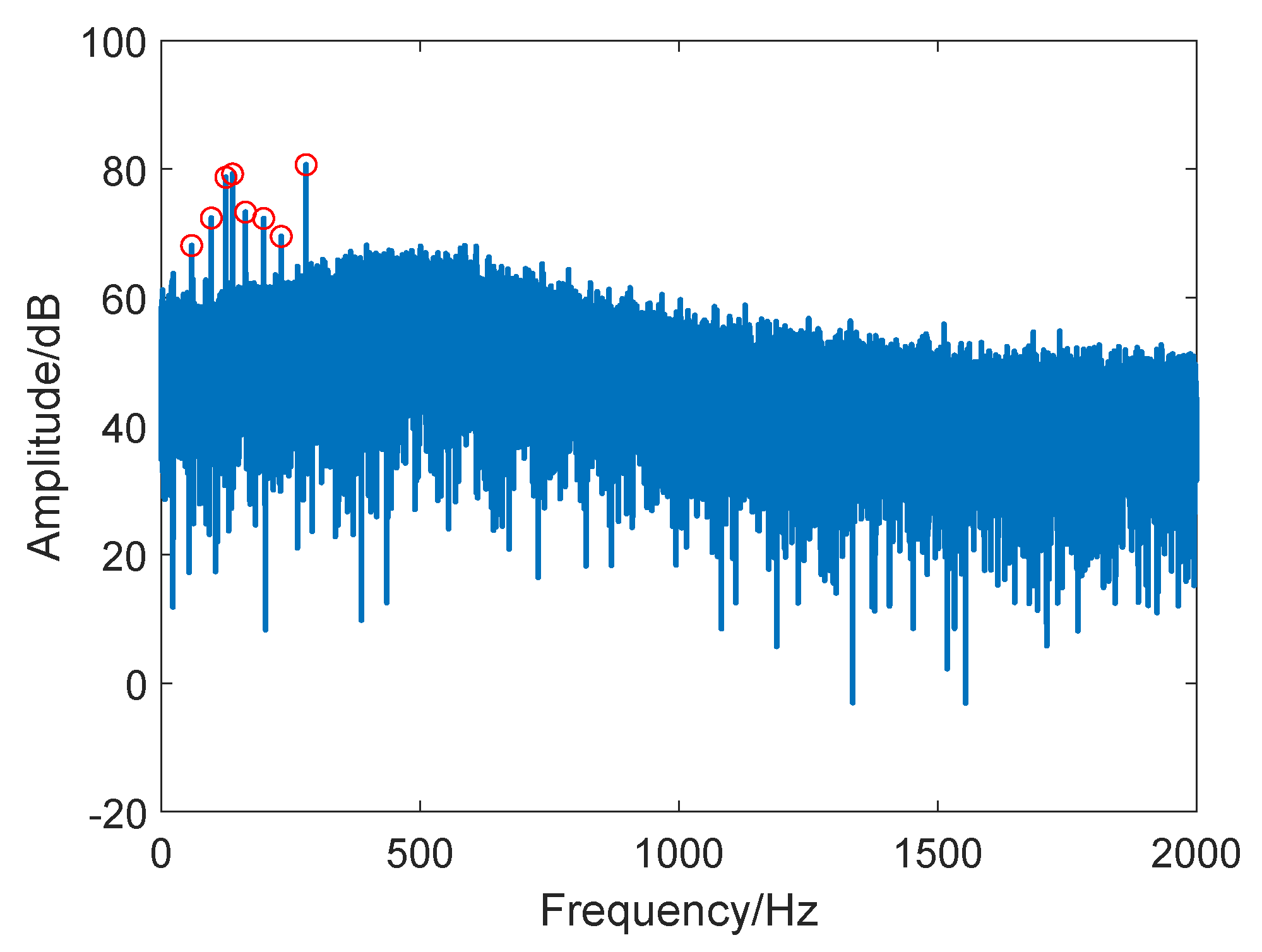
3.1. Phase Extraction Based on Detected Narrow-Band Frequencies

Assume a passive sonar system with the sample rate of $F_s$ and the time interval of T, and thus the total number of sample is $N=F_{s}T$. In accordance with Equation (6), the observed signal $y_m\left(t\right)$ at the mth sensor is decomposed into N narrow-band components using Discrete Fourier Transform (DFT). The resulting narrow-band components corresponding to any one of the frequency points may be expressed as,

$$\begin{array}{c}\hfill y_m\left(f_n\right)=\sum _{k=1}^K{\zeta }_{k,m}\left(f_n\right)s_k\left(f_n\right)exp(-j2\pi f_n{\tau }_{k,m})+e_m\left(f_n\right),n\in (1,\cdots ,N),\end{array}$$

(9)

where $f_n=n{F}_s/N$ is the nth frequency grid, ${\zeta }_{k,m}\left(f_n\right)$ is the coefficient at the $f_n$ frequency with a high value, when a strong sinusoidal noise signal at the frequency of $f_n$ exists, and K is the number of the far-field sources of opportunity.

According to Equation (9), the wideband beamforming is turned to be multiple narrow-band beamforming through the DFT procedure. The weight vector with the pre-defined ${\vartheta }_q$ in the nth frequency point is written by,

$$\begin{array}{c}\hfill \mathbf{w}(f_n,{\vartheta }_q)={\left[1,exp\left(\frac{-j2\pi f_{n}dcos{\vartheta }_q}{v}\right)\cdots ,exp\left(\frac{-j2\pi f_n(M-1)dcos{\vartheta }_q}{v}\right)\right]}^T,\end{array}$$

(10)

where ${\vartheta }_q\in (0,180)$, $q\in 1,\cdots ,Q$, and Q is the number of the pre-defined bearing grid. According to weights in Equation (10), beamforming is achieved by

$$\begin{array}{c}\hfill \varrho \left({\vartheta }_k\right)=\sum _{n=1}^N{\left|\mathbf{w}{(f_n,{\vartheta }_k)}^H\mathbf{y}\left(f_n\right)\right|}^2,k\in 1,\cdots ,Q,\end{array}$$

(11)

where $\mathbf{y}\left(f_n\right)={[y_1\left(f_n\right),\cdots ,y_M\left(f_n\right)]}^T\in {\mathcal{C}}^M$ is a received signal vector in the nth frequency point. According to the result in Equation (11), the ${\widehat{\vartheta }}_k$ is estimated based on the maximum-value detection criterion. The output signal based on the estimated ${\widehat{\vartheta }}_k$ is,

$$\begin{array}{c}\hfill {\tilde{y}}_k\left(n\right)=\sum _{m=1}^M{y}_m\left[n-\frac{(m-1)dcos{\widehat{\vartheta }}_k}{v}\right],n\in (1,\cdots ,N),\end{array}$$

(12)

where M is the number of the hydrophone sensors.

The operations above in Equations (9)–(12) are involved in the basic wideband frequency beamforming method. The weight vector in Equation (10) is optimal, and the signal to noise ratio (SNR) of the output signal ${\tilde{\mathbf{y}}}_k={[{\tilde{y}}_k\left(1\right),\cdots ,{\tilde{y}}_k\left(N\right)]}^T$ can be improved by M times, when the array is nominally uniform linear in the Gaussian noise case. However, the array should be deformed severely and not remain a straight line due to the transverse motion of the towing vessel, oceanic currents, and hydrodynamic effects, weights in Equation (10) would be wrong. Therefore, the performance of beamforming would worsen dramatically, when the hydrophone array greatly deviates from the nominal one. Taking a uniform linear towed array of $M=128$ hydrophone sensors with a spatial interval of $1.6$ m for example, the shape of the distorted array approximately becomes a parabola and deviation angle ${\varphi }_m$ is $sin(\pi /(2M\left)\right)$, the average loss of the narrow-band signals would reach up to about 15 dB.

The output signal ${\tilde{\mathbf{y}}}_k$ based on the nominal array shape would not be the optimal one in the distorted array cases because the time delays in the weight vector Equation (10) do not match the true ones. Considering the fact that an important component in radiated noise originates from the machinery noise and can be regarded as the superposition of multiple narrowband signals, we would utilize the phases of these narrow-band signals to estimate time delays in the distorted array instead of the time delays in the nominal array. Instead of directly performing the element-space narrow-band detection, we carry out the detection on the spectrum of $P_{yk}\left(f\right)$, which is acquired by performing the DFT operation on the output signal ${\tilde{\mathbf{y}}}_k$. By exploiting the background calibration and threshold-based detection techniques, the detected narrow-band frequencies radiated by the kth source of opportunity can be denoted as ${\widehat{f}}_{kl}$ with $l\in 1,\cdots ,L_0$, where $L_0$ is the number of detected narrow-band frequencies. The corresponding unwrapped phase of the lth narrow-band frequency from the kth source to the mth sensor can be acquired by,

$$\begin{array}{c}\hfill {\psi }_m\left({\widehat{f}}_{kl}\right)=2\pi {\widehat{f}}_{kl}{\tau }_{k,m}.\end{array}$$

(13)

In a similar way, we obtain the phase of ${\psi }_{m+1}\left({\widehat{f}}_{kl}\right)$ in the $(m+1)$th hydrophone, and thus estimate the adjacent phase difference by

$$\begin{array}{c}\hfill \Delta {\widehat{\psi }}_{k,l,m}={\psi }_{m+1}\left({\widehat{f}}_{kl}\right)-{\psi }_m\left({\widehat{f}}_{kl}\right),l\in 1,\cdots ,L_0.\end{array}$$

(14)

$$\begin{array}{c}\hfill \Delta {\widehat{\tau }}_{k,l,m}=\frac{{\psi }_{m+1}\left({\widehat{f}}_{kl}\right)-{\psi }_m\left({\widehat{f}}_{kl}\right)}{2\pi {\widehat{f}}_{kl}},l\in 1,\cdots ,L_0.\end{array}$$

(15)

3.2. Proposed Weighted Outlier-Robust Kalman Smoother

Ideally, the estimated time-delay difference $\Delta {\widehat{\tau }}_{k,l,m}$ between the $(m+1)$th hydrophone sensor the mth hydrophone sensor expressed by Equation (14) should be independent of narrow-band frequencies, and be identical among $L_0$ narrow-band frequencies. The reason is that its phase difference is only determined by the spatial interval d between adjacent hydrophones and the bearing of impinging source. However, the time-delay differences $\Delta {\widehat{\tau }}_{k,l,m}$ with $l\in 1,\cdots ,L_0$ are often diverse in the real case. Figure 3 shows an example in a public SWellEx-96 HLA dataset [22]. It is observed that the time-delay differences in the detected narrow-band frequencies are completely different across sensors. The possible reason is that there are diverse SINRs in these detected narrow-band frequencies, and these time-delay differences will deviate from the true values at these frequencies.

One way to alleviate the fluctuations of $\Delta {\widehat{\tau }}_{k,l,m}$ is average these estimated time-delay differences and acquire [23]

$$\begin{array}{c}\hfill \Delta {\widehat{\tau }}_{k,m}=\frac{1}{L_0}\sum _{l=1}^{L_0}\Delta {\widehat{\tau }}_{k,l,m},m\in 0,\cdots ,M-2.\end{array}$$

(16)

However, the average operator being a linear estimator is sensitive to outliers and easily deviates from the true value when there exists a small number of outliers. The $\Delta {\widehat{\tau }}_{k,l,m}$ acquired by the adjacent phase differences easily deteriorates in the low SINR cases, and thus become abnormal. In this case, these outliers would lead to a large deviation in the average operator. Therefore, the average operator is not an optimal way to acquire the time-delay estimation in the distorted array. To address this issue, we propose to use a weighted robust-outlier Kalman smoother.

Instead of averaging all the $\Delta {\widehat{\psi }}_{k,l,m}$ in multiple narrow-band frequencies, we stack $\Delta {\widehat{\psi }}_{k,l,m}$ with $l=1,\cdots ,L_0$ into a vector as ${\mathbf{z}}_{k,m}={\left[\Delta {\widehat{\psi }}_{k,1,m},\cdots ,\Delta {\widehat{\psi }}_{k,L_0,m}\right]}^T$, and regard ${\mathbf{z}}_{k,m}$ as the observation data sample. In conformity with the analysis above, the observation equation is expressed by,

$$\begin{array}{c}\hfill {\mathbf{z}}_{k,m}=\mathit{\alpha }\left(f\right)\times \Delta {\tau }_{k,m}+{\mathit{ϵ}}_m,\end{array}$$

(17)

where $\mathit{\alpha }\left(f\right)={\left[2\pi f_1,\cdots ,2\pi f_{L_0}\right]}^T\in {\mathcal{R}}^{L_0\times 1}$ is a vector, $\Delta {\tau }_{k,m}$ is the true time-delay difference between the $(m+1)$th and the mth sensors, and ${\mathit{ϵ}}_m\in {\mathcal{R}}^{L_0\times 1}$ is an additive noise.

According to Equation (17), the observed time-delay differences in multiple narrow-band frequencies can be considered as the true time-delay difference plus noise. To alleviate the effects of outliers and diverse noise levels in the multiple frequencies, we introduce a novel Bayesian algorithm that treats the weights associated with each observation data samples probabilistically as proposed by [24,25]. However, unlike [24,25] which use a scalar to weight the observed data sample and all elements in observed data sample are equally treated, we introduce a vector weight ${\mathit{\gamma }}_m$ for each observed data sample ${\mathbf{z}}_{k,m}$ such that the variances of ${\mathbf{z}}_{k,m}$ are weighted with ${\mathit{\gamma }}_m$, owing to diverse SINRs in the corresponding narrow-band frequencies, and have,

$$\begin{array}{c}\hfill {\mathbf{z}}_{k,m}|{\mathit{\gamma }}_m,\mathbf{r}\sim \mathcal{N}\left({\mathbf{z}}_{k,m}|\mathit{\alpha }\left(f\right)\Delta {\tau }_{k,m},{\mathsf{\Gamma }}_m^{-1}\mathbf{R}\right),\end{array}$$

(18)

where $\mathbf{R}=\mathrm{diag}\left(\mathbf{r}\right)$, which is a covariance matrix for observation noise, is a diagonal matrix with $\mathbf{r}={\left[r_1,\cdots ,r_{L_0}\right]}^T\in {\mathcal{R}}^{L_0\times 1}$ on its diagonal. ${\mathsf{\Gamma }}_m=\mathrm{diag}\left({\mathit{\gamma }}_m\right)$ is a diagonal matrix with ${\mathit{\gamma }}_m={\left[{\gamma }_{1m},\cdots ,{\gamma }_{L_{0}m}\right]}^T\in {\mathcal{R}}^{L_0\times 1}$ on its diagonal. It should be noted that each elements in $\mathbf{r}$ is weighted by the corresponding ${\mathit{\gamma }}_m$. A Gamma prior distribution for the weights in order to ensure they remain positive is imposed on the weight vector ${\mathit{\gamma }}_m$ as,

$$\begin{array}{c}\hfill {\gamma }_{lm}\sim \mathrm{Gamma}\left({\gamma }_{lm}|a_0,b_0\right),l=1,\cdots ,L_0,m=0,\cdots ,M-2,\end{array}$$

(19)

where Gamma(·) represents a Gamma distribution, and $a_0$ and $b_0$ are hyperparameters respectively, and often set to $a_0=b_0$.

Considering the fact that external shell of hydrophone array is soft and elastic, it is reasonable to assume the time-delay differences $\Delta {\tau }_{k,m}$ are slowly changing across sensors (These ${\Delta \tau }_{k,m}$ with $m=0,\cdots ,M-2$ should be identical, when the array is ideally straight), and thus we have the state equation as

$$\begin{array}{c}\hfill \Delta {\tau }_{k,m+1}=\Delta {\tau }_{k,m}+{\epsilon }_m,m=0,\cdots ,M-2,\end{array}$$

(20)

where $\Delta {\tau }_{k,m+1}$ is the time-delay difference between the $(m+2)$th sensor and the $(m+1)$th sensor, and ${\epsilon }_m$ is an additive noise. For the $m=0$, the initialization of $\Delta {\tau }_{k,0}$ is assumed to follow the Gaussian distribution of $\Delta {\tau }_{k,0}\sim \mathcal{N}\left(\Delta {\tau }_{k,0}|0,{\nu }_0\right)$. Without loss of generality, a Gaussian prior is considered to model this noise, and can be expressed by,

$$\begin{array}{c}\hfill {\epsilon }_m|\nu \sim \mathcal{N}\left({\epsilon }_m|0,\nu \right),\end{array}$$

(21)

where $\nu$ is the variance of state noise.

In accordance with these time-delay differences in the M sensors, we have observed data samples $\Delta {\tau }_{k,0:M-2}$ at one time. To estimate the posterior distributions of the random variables and parameter values, we should consider the log evidence of the data samples observed, i.e., $logp\left({\mathbf{z}}_{k,0:M-2},\Delta {\tau }_{k,0:M-2},{\mathit{\gamma }}_{0:M-2}\right)$. It is a typical Kalman smoother.

We can treat this entire problem as an Expectation Minimization (EM) learning problem [26]. The expectation of the complete data likelihood should be taken with respect to the true posterior distribution of all hidden variables $q\left(\Delta {\tau }_{k,0:M-2},{\mathit{\gamma }}_{0:M-2}\right)$. However, since this is an analytically intractable expression, we make a factorial approximation of the true posterior as follows [27],

$$\begin{array}{c}\hfill q\left(\Delta {\tau }_{k,0:M-2},{\mathit{\gamma }}_{0:M-2}\right)=\prod _{m=0}^{M-2}q\left({\mathit{\gamma }}_m\right)\prod _{m=0}^{M-3}q\left(\Delta {\tau }_{k,m+1}|\Delta {\tau }_{k,m}\right)q\left(\Delta {\tau }_{k,0}\right).\end{array}$$

(22)

This factorization of $\Delta {\tau }_{k,0:M-2}$ considers the influence of each $\Delta {\tau }_{k,m}$ within its Markov chain. According to this factor approximation, all resulting posterior distributions over hidden variables become analytically tractable. We can derive the final EM update equations from standard manipulations of Gaussian and Gamma distributions and acquire the following,

$\mathrm{E}\text{-}\mathrm{step}:$

Forward recursion,

$$\begin{array}{cc}\hfill & \mathcal{N}\left(\Delta {\tau }_{k,m}|{\mu }_m,v_m\right)\propto \mathcal{N}\left({\mathbf{z}}_{k,m}|\mathit{\alpha }\left(f\right)\Delta {\tau }_{k,m},{\mathsf{\Gamma }}^{-1}\mathbf{R}\right)\mathcal{N}\left(\Delta {\tau }_{k,m}|{\mu }_{m-1},〈\nu 〉+v_{m-1}\right),\hfill \end{array}$$

(23)

$$\begin{array}{cc}\hfill & \to {\mu }_m=v_m\left(\sum _{l=1}^{L_0}\frac{〈{\gamma }_{lm}〉}{〈r_l〉}{z}_{k,m,l}+\frac{2\pi f_l{\mu }_{m-1}}{〈\nu 〉+v_{m-1}}\right),\hfill \end{array}$$

(24)

$$\begin{array}{cc}\hfill & \to v_m={\left(\sum _{l=1}^{L_0}\frac{〈{\gamma }_{lm}〉}{〈r_l〉}+\frac{1}{〈\nu 〉+v_{m-1}}\right)}^{-1},\hfill \end{array}$$

(25)

$$\begin{array}{cc}\hfill & \to 〈{\gamma }_{lm}〉=\frac{a_0+1/2}{\frac{1}{2〈r_l〉}{\left(z_{k,m,l}-2\pi f_l{\mu }_m\right)}^2+b_0}l\in \{1,\cdots ,L_0\}.\hfill \end{array}$$

(26)

Backward recursion,

$$\begin{array}{cc}\hfill & \widehat{\gamma }\left(\Delta {\tau }_{k,m}\right)=\mathcal{N}\left(\Delta {\tau }_{k,m}|{\widehat{\mu }}_m,{\widehat{v}}_m\right)\propto \mathcal{N}\left({\widehat{\mu }}_{m+1}|\Delta {\tau }_{k,m},〈\nu 〉\right)\mathcal{N}\left(\Delta {\tau }_{k,m}|{\mu }_m,v_m\right),\hfill \end{array}$$

(27)

$$\begin{array}{cc}\hfill & \to {\widehat{\mu }}_m={\widehat{v}}_m\left(\frac{{\mu }_m}{v_m}+\frac{{\widehat{\mu }}_{m+1}}{〈\nu 〉}\right)={\mu }_m+\frac{v_m}{v_m+〈\nu 〉}\left({\widehat{\mu }}_{m+1}-{\mu }_m\right),\hfill \end{array}$$

(28)

$$\begin{array}{cc}\hfill & \to {\widehat{v}}_m=v_m+\frac{v_m^2}{{\left(v_m+〈\nu 〉\right)}^2}\left[{\widehat{v}}_{m+1}-(v_m+〈\nu 〉)\right].\hfill \end{array}$$

(29)

$\mathrm{M}\text{-}\mathrm{step}:$

$$\begin{array}{cc}\hfill 〈r_l〉& =\sum _{i=1}^m\frac{〈{\gamma }_{li}〉}{m}{\left(z_{k,i,l}-〈\Delta {\tau }_{k,i}〉\right)}^2,\hfill \end{array}$$

(30)

$$\begin{array}{cc}\hfill 〈\nu 〉& =\sum _{i=1}^m\frac{1}{m}{\left(〈\Delta {\tau }_{k,i}〉-〈\Delta {\tau }_{k,i-1}〉\right)}^2.\hfill \end{array}$$

(31)

Once these time-delay differences ${\left\{{\mu }_m\right\}}_{m=0}^{M-1}$ have been obtained, we can estimate the array shape. Since the first two sensors define the the baseline, the estimated bearing ${\widehat{\vartheta }}_k$ of the kth noise source can be calculated based on the estimated time-delay ${\widehat{\mu }}_0$ according to Equation (3),

$$\begin{array}{c}\hfill {\widehat{\vartheta }}_k=arccos\left(\frac{v{\widehat{\mu }}_1}{d}\right).\end{array}$$

(32)

Therefore, the estimated deviation angle ${\widehat{\varphi }}_m$ can be calculated as according to Equation (3),

$$\begin{array}{c}\hfill {\widehat{\varphi }}_m=arccos\left(\frac{v{\widehat{\mu }}_1}{d}\right)-arccos\left(\frac{v{\widehat{\mu }}_m}{d}\right)\end{array}$$

(33)

The location $({\widehat{x}}_{m+1},{\widehat{y}}_{m+1})$ of $(m+1)$th sensor can be estimated by,

$$\begin{array}{cc}\hfill {\widehat{x}}_{m+1}& ={\widehat{x}}_m+v{\widehat{\mu }}_{m}cos\left({\widehat{\varphi }}_m\right)+\sqrt{d^2-v^2{\widehat{\mu }}_m^2}sin\left({\widehat{\varphi }}_m\right)\hfill \end{array}$$

(34)

$$\begin{array}{cc}\hfill {\widehat{y}}_{m+1}& ={\widehat{y}}_m+v{\widehat{\mu }}_{m}sin\left({\widehat{\varphi }}_m\right)+\sqrt{d^2-v^2{\widehat{\mu }}_m^2}cos\left({\widehat{\varphi }}_m\right),\hfill \end{array}$$

(35)

where $m=2,\cdots ,M-1$.

Finally, we perform the beamforming and acquire the improved output signal based on the estimated array shape as

$$\begin{array}{c}\hfill {\overline{y}}_k\left(n\right)=y_1+\sum _{m=1}^{M-1}{y}_m\left[n-\sum _{i=1}^m{\widehat{\mu }}_{i-1}\right],\end{array}$$

(36)

where $n=[1,\cdots ,N]$.

3.3. Summary of Proposed Distorted Array Shape Estimation Scheme

The proposed distorted array shape estimation scheme is summarized in

Table 1. Summary of Proposed Distorted Array Shape Estimation Scheme.

Given the observed array data ${\left\{y_m\left(t\right)\right\}}_{m=1}^M$.

(1) Calculate ${\tilde{\mathbf{y}}}_k$ with respect to the kth source based on the hypothetical uniform linear array.

(2) Acquire the detected narrow-band frequencies ${\widehat{f}}_{kl}$ with $l\in 1,\cdots ,L_0$ based on $y_m\left(t\right)$.

(3) Calculate time-delay differences vector ${\mathbf{z}}_{k,m}={\left[\Delta {\widehat{\psi }}_{k,1,m},\cdots ,\Delta {\widehat{\psi }}_{k,L_0,m}\right]}^T,m=0,\cdots ,M-2$.

(4) Estimate the time-delay differences using proposed Weighted Robust-Outlier Kalman Smoother:

a. Initialize hyperparameters $a_0$ and $b_0$.

b. Initialize covariance for observation noise $\mathbf{R}$, variance of state noise $\nu$.

c. Estimate time-delay differences ${\widehat{\mu }}_m$ using EM algorithm Equations (23)–(30).

(5) Perform array shape estimates $({\widehat{x}}_m,{\widehat{y}}_m)$ with $m=2,\cdots ,M-1$ using Equations (34) and (35).

(6) Perform the beamforming and acquire the improved output signal ${\overline{y}}_k\left(t\right)$.

.

3.4. Performance Bound Analysis

To quantify the estimation performance of the proposed method, we perform the CRLB analysis in this section. Considering the problem of estimating the time-delay difference vector $\Delta {\mathit{\tau }}_k={\left[\Delta {\tau }_{k,0},\cdots ,\Delta {\tau }_{k,M-2}\right]}^T$ from a set of observed data vectors of ${\mathbf{z}}_k={\left[{\mathbf{z}}_{k,0}^T,\cdots ,{\mathbf{z}}_{k,M-2}^T\right]}^T$ with ${\mathbf{z}}_{k,m}={\left[\Delta {\widehat{\psi }}_{k,1,m},\cdots ,\Delta {\widehat{\psi }}_{k,L_0,m}\right]}^T$, we can acquire the joint probability distribution function (pdf) $p(\Delta {\mathit{\tau }}_k,{\mathbf{z}}_k)$ from the kth source as based on Equations (18) and (20),

$$\begin{array}{cc}\hfill p\left(\Delta {\mathit{\tau }}_k,{\mathbf{z}}_k\right)={\int }_{{\mathit{\gamma }}_m}& {\displaystyle \prod _{m=0}^{M-2}}\mathcal{N}\left({\mathbf{z}}_{k,m}|\mathit{\alpha }\left(f\right)\Delta {\tau }_{k,m},{\mathsf{\Gamma }}_m^{-1}\mathbf{R}\right)\mathcal{N}\left(\Delta {\tau }_{k,m+1}|\Delta {\tau }_{k,m},\nu \right)\hfill \\ \hfill & \times \mathcal{N}\left(\Delta {\tau }_{k,0}|0,{\nu }_0\right)\mathrm{Gamma}\left({\mathit{\gamma }}_m|a_0,b_0\right)d{\mathit{\gamma }}_m.\hfill \end{array}$$

(37)

The Fisher information matrix (FIM) $\mathbf{J}(\Delta {\mathit{\tau }}_k)$ for the parameter vector $\Delta {\mathit{\tau }}_k$ is defined as follows,

$$\begin{array}{c}\hfill \mathbf{J}(\Delta {\mathit{\tau }}_k)=-\mathbb{E}\left\{{\nabla }_{\Delta {\mathit{\tau }}_k}{\left[{\nabla }_{\Delta {\mathit{\tau }}_k}lnp({\Delta \mathit{\tau }}_k,{\mathbf{z}}_k)\right]}^T\right\}.\end{array}$$

(38)

When the derivatives and expectation exist, we acquire an alternative formula for the FIM as,

$$\begin{array}{c}\hfill \mathbf{J}(\Delta {\mathit{\tau }}_k)=\mathbb{E}\left\{{\left[{\nabla }_{\Delta {\mathit{\tau }}_k}lnp({\Delta \mathit{\tau }}_k,{\mathbf{z}}_k)\right]}^T{\nabla }_{\Delta {\mathit{\tau }}_k}lnp(\Delta {\mathit{\tau }}_k,{\mathbf{z}}_k)\right\}.\end{array}$$

(39)

Let $\Delta {\widehat{\mathit{\tau }}}_k=\Delta {\widehat{\mathit{\tau }}}_k\left({\mathbf{z}}_k\right)$ be an estimated of the parameter vector $\Delta {\tau }_k$. The mean-square error matrix (MSEM) is defined as

$$\begin{array}{c}\hfill {\mathsf{\Xi }}_k\left(\Delta {\widehat{\mathit{\tau }}}_k\right)=\mathbb{E}\left[\left(\Delta {\mathit{\tau }}_k-\Delta {\widehat{\mathit{\tau }}}_k\right){\left(\Delta {\mathit{\tau }}_k-\Delta {\widehat{\mathit{\tau }}}_k\right)}^T\right].\end{array}$$

(40)

In fact, the MSEM is bounded by an inverse of the FIM, and we acquire [28],

$$\begin{array}{c}\hfill {\mathsf{\Xi }}_k\left(\Delta {\widehat{\mathit{\tau }}}_k\right)\ge {\mathbf{J}}^{-1}\left(\Delta {\mathit{\tau }}_k\right).\end{array}$$

(41)

The inverse of ${\mathbf{J}}^{-1}\left(\Delta {\mathit{\tau }}_k\right)$ is just the well-known posterior or Bayesian Cramer–Rao bound [29], and it will be denoted as $\mathbf{C}(\Delta {\mathit{\tau }}_k)$. According to the proposed generative model in Section 3.2, the logarithm of joint pdf of the state and measurement histories $p({\mathbf{z}}_k,\Delta {\mathit{\tau }}_k)$ can be expressed as,

$$\begin{array}{c}\hfill lnp\left({\mathbf{z}}_k,\Delta {\tau }_k\right)=\sum _{m=0}^{M-2}lnp\left({\mathbf{z}}_{k,m}|\Delta {\tau }_{k,m}\right)+\sum _{m=1}^{M-2}lnp\left(\Delta {\tau }_{k,m}|\Delta {\tau }_{k,m-1}\right)+lnp\left(\Delta {\tau }_{k,0}\right).\end{array}$$

(42)

Motivated by [28], we follow a similar recursive approach for the smoothing CRLBs, and express CRLBs for the filtering as in the forward recursion,

$$\begin{array}{cc}\hfill C_{m|m}^{-1}& =C_{m|m-1}^{-1}+S_m^m,\hfill \end{array}$$

(43)

$$\begin{array}{cc}\hfill C_{m+1|m}^{-1}& =G_{m+1}^{m+1}-G_{m+1}^{m+1,m}{(G_{m+1}^m+C_{m|m}^{-1})}^{-1}{G}_{m+1}^{m+1,m},\hfill \end{array}$$

(44)

$$\begin{array}{cc}\hfill C_{0|-1}^{-1}& =G_0^0,\hfill \end{array}$$

(45)

where $m=0,\cdots ,M-2$. We acquire the CRLBs of the smoother in the backward recursion [28],

$$\begin{array}{c}\hfill C_{m|M-2}^{-1}=C_{m|m}^{-1}+G_{m+1}^m-G_{m+1}^{m+1,m}{(G_{m+1}^{m+1}+C_{m+1|M-2}^{-1}+C_{m+1|m}^{-1})}^{-1}{G}_{m+1}^{m+1,m}.\end{array}$$

(46)

where,

$$\begin{array}{cc}\hfill G_{m+1}^m& =\mathbb{E}\left\{-{\nabla }_{\Delta {\tau }_{k,m}}\left[{\nabla }_{\Delta {\tau }_{k,m}}lnp\left(\Delta {\tau }_{k,m+1}|\Delta {\tau }_{k,m}\right)\right]\right\},\hfill \end{array}$$

(47)

$$\begin{array}{cc}\hfill G_{m+1}^{m,m+1}& =\mathbb{E}\left\{-{\nabla }_{\Delta {\tau }_{k,m+1}}\left[{\nabla }_{\Delta {\tau }_{k,m}}lnp\left(\Delta {\tau }_{k,m+1}|\Delta {\tau }_{k,m}\right)\right]\right\},\hfill \end{array}$$

(48)

$$\begin{array}{cc}\hfill G_{m+1}^{m+1}& =\mathbb{E}\left\{-{\nabla }_{\Delta {\tau }_{k,m+1}}\left[{\nabla }_{\Delta {\tau }_{k,m+1}}lnp\left(\Delta {\tau }_{k,m+1}|\Delta {\tau }_{k,m}\right)\right]\right\},\hfill \end{array}$$

(49)

$$\begin{array}{cc}\hfill S_m^m& =\mathbb{E}\left\{-{\nabla }_{\Delta {\tau }_{k,m}}\left[{\nabla }_{\Delta {\tau }_{k,m}}lnp\left({\mathbf{z}}_{k,m}|\Delta {\tau }_{k,m}\right)\right]\right\}.\hfill \end{array}$$

(50)

According to Equations (18) and (19) in the generative model, $p\left({\mathbf{z}}_{k,m}\right)$ would follow a multivariate Student distribution by integrating the weight vector ${\mathit{\gamma }}_m$, and can be expressed by,

$$\begin{array}{c}\hfill {\mathbf{z}}_{k,m}|\Delta {\tau }_{k,m},\sim \mathrm{st}\left(\mathit{\alpha }\left(f\right)\Delta {\tau }_{k,m},\mathbf{R},\upsilon \right),\end{array}$$

(51)

where $\mathrm{st}(·)$ denotes the student-t distribution, and the freedom $\upsilon =2a_0$.

According to [28], we derive the recursive formula for the CRLB of the proposed WORKS method as in the forward recursion,

$$\begin{array}{cc}\hfill C_{m|m}^{-1}& =C_{m|m-1}^{-1}+\frac{\upsilon +L}{\upsilon +L+2}\mathit{\alpha }{\left(f\right)}^H{\mathbf{R}}^{-1}\mathit{\alpha }\left(f\right),\hfill \end{array}$$

(52)

$$\begin{array}{cc}\hfill C_{m+1|m}^{-1}& ={\nu }^{-1}-{\nu }^{-1}{({\nu }^{-1}+C_{m|m}^{-1})}^{-1}{\nu }^{-1},\hfill \end{array}$$

(53)

$$\begin{array}{cc}\hfill C_{0|-1}^{-1}& ={\nu }_{k,0}.\hfill \end{array}$$

(54)

and we acquire the corresponding recursive formula for the CRLB as in the backward recursion,

$$\begin{array}{c}\hfill C_{m|M-2}^{-1}=C_{m|m}^{-1}+{\nu }^{-1}-{\nu }^{-1}{({\nu }^{-1}+C_{m+1|M-2}^{-1}+C_{m+1|m}^{-1})}^{-1}{\nu }^{-1},\end{array}$$

(55)

where $m=0,\cdots ,M-2$.

4. Simulations and Experiments

In this section, both simulations and experiments will verify the effectiveness and correctness of the proposed method. Several typical source-dependent approaches, such as subspace-based eigenvector method [11] and average operation [23], are used for comparisons in simulations and experiments.

4.1. Simulations

Suppose that a uniform linear towing array has $M=128$ hydrophone sensors with a spatial interval of $1.6$ m, and the bearing of a radiated noise source is ${60}^{\circ }$. The deviation angle ${\varphi }_m$ is set to be $sin(\pi /(2M\left)\right)$, and thus the shape of the distorted array approximately becomes a parabola, as the black line shown in Figure 4a. The time duration is $T=5$ s and the sampling rate $F_s=4$ kHz. According to the characteristics of radiated noise [20,21], a three parameters model with $f_c=500$ Hz, $f_m=200$ Hz and $\kappa =0$ is used to model the continuous spectrum component. In addition, seven narrow-band (sinusoid) signals with frequencies of 59 Hz, 97 Hz, 125 Hz, 163 Hz, 198 Hz, 232 Hz and 280 Hz are considered. Without loss of generality, additive Gaussian noise and additional interferences in three narrow-band frequencies with 59 Hz, 97 Hz, and 163 Hz are considered with the SINR of $-10$ dB.

Figure 4b shows the beamforming result based on the hypothetical uniform linear array. The maximum value in the beam energy diagram is ${55}^{\circ }$, which is deviated from the true bearing of ${60}^{\circ }$, due to the time-delay mismatches in the distorted array. Only five narrow-band frequencies with 59 Hz, 97 Hz, 198 Hz, 163 Hz, and 232 Hz are acquired after the narrow-band detection based on the beamforming with the hypothetical array shape, and the narrow-band frequencies with 125 Hz and 280 Hz are missing. The corresponding time-delay differences of these detected narrow-band frequencies with 59 Hz, 97 Hz, 163 Hz, 198 Hz, and 232 Hz are shown in Figure 4d. It is observed that the time-delay differences are generally different, and show significant fluctuations particularly in the frequencies of 59 Hz, 97 Hz, and 163 Hz, due to the diverse SINRs on these narrow-band frequencies. Several outliers appear in the estimated time-delay differences. The time-delay differences should be independent of the considered narrow-band frequencies and be identical for the five narrow-band frequencies.

The ground truth of time-delay differences is shown in Figure 4c with the black line, while the average of these phase differences is shown in Figure 4c with the blue line. The estimation of time-delay differences in the subspace method is shown in Figure 4c with the green line. It is found that the estimates of time-delay differences in both the subspace-based method and the average operation method exhibit relatively large deviations from the ground truth and lead to quite similar estimates of the time-delay differences. The possible reason is that both the subspace-based method and the average operation approach are based on the narrow-band phase differences between adjacent elements, and both of them utilize the average operators for the estimates of time-delay differences in essence. The estimated time-delay differences in the proposed WORKS method, which significantly inhibits outliers, are quite closer to the true values, as shown in Figure 4c with the red line. According to the detected narrow-band frequencies, the array shape estimation is acquired by Equations (34) and (35), as shown in Figure 4a. The estimated array shape in the proposed method is closer to the real one, compared to those of the other two methods, even if gaps exist between them, especially in the latter part of the array. It is due to the error accumulations of time-delay differences in the array shape estimation, according to Equation (5).

The output spectrum based on the estimated array shape is provided in Figure 4e. It is reasonable that the output spectrum has higher gain, and is closer to the spectrum in the known array shape, compared to these in the subspace method and average operation method. It is also observed that the missing narrow-band frequency of 125 Hz becomes quite clear and can easily be detected in this enhanced spectrum. To quantify the superior performance, we use the amplitude error as the performance index. The amplitude error is defined as the absolute error between the amplitude of the detected narrow-band frequency and the amplitude in the corresponding frequencies in the spectrum based on the known array shape. The amplitude errors of the three methods are presented in

Table 2. Amplitude errors of detected narrow-band frequencies.

Frequency/Hz	59	97	125	163	198	232	280
Amplitude error in average method/dB	25.3	15.0	43.2	24.6	37.9	11.4	25.2
Amplitude error in subspace method/dB	24.9	15.7	49.7	24.8	32.8	11.3	22.6
Amplitude error in proposed method/dB	0.1	0.1	0.1	0.1	0.2	0.3	0.3

. It is obvious that the proposed method is superior over the average operation and the subspace-based methods, owing to the ability to mitigate the effects of the outliers. It is also observed that the proposed method generally has the highest gain improvements among these three methods, and its amplitude errors in these detected narrow-band frequencies are generally less than $0.3$ dB.

4.1.1. Variance Estimates of Time-Delay Difference

In this subsection, the variance estimates of time-delay differences are analyzed. All the parameters are the same as the simulations above. Figure 5 shows the variance results of the estimated $\Delta \tau$. It is obvious that the proposed approach has the lowest estimated variance across 128 sensors, and its average variance is 0.023, which is quite closer to the CRBL of 0.006, compared to 0.842 and 0.821 in the average operation and the subspace-based methods, respectively. The main reason is that the proposed method is quite robust to these outliers in the estimated time-delay differences possibly caused by the low-SNR phases, whereas both average operation and the subspace-based method are sensitive to these outliers, and would lead to relatively poor performance.

4.1.2. Performance Comparison versus Bearings of the Radiated Noise Source

The effectiveness of the proposed method has been verified thanks to the aforementioned simulations. In the following simulation, the performance versus bearings of the noise source will be analyzed. The source bearings change from $5^{\circ }$ to ${175}^{\circ }$ by ${10}^{\circ }$ steps. Other parameters are the same as in the previous simulations. It is observed that all three approaches seem robust to the bearings of targets and their average gain errors of narrow-band frequencies in the end-fire bearing are comparable to those in the upright bearing. However, the average gain errors of results in the proposed method are much smaller than in the average operation and the subspace-based methods, as shown in Figure 6.

4.1.3. Performance Comparison versus SINR

In this simulation, we focus on the performance comparison versus diverse SINRs. The narrow-band frequency interferences of 59 Hz, 97 Hz, and 163 Hz with different amplitudes, which would cause diverse outliers in time-delay differences, are considered to form diverse SINRs from $-3$ dB to $-14$ dB with the step of $-2$ dB. Figure 7 shows average amplitude errors versus diverse SINRs. The proposed method has superior performance over the average operation and the subspace-based methods. It is observed that the average amplitude errors of the subspace-based method and the average operation approach gradually increase as the SINR decreases, whereas the proposed method is robust to different SINRs, which means the proposed method could mitigate the effects of different SINRs.

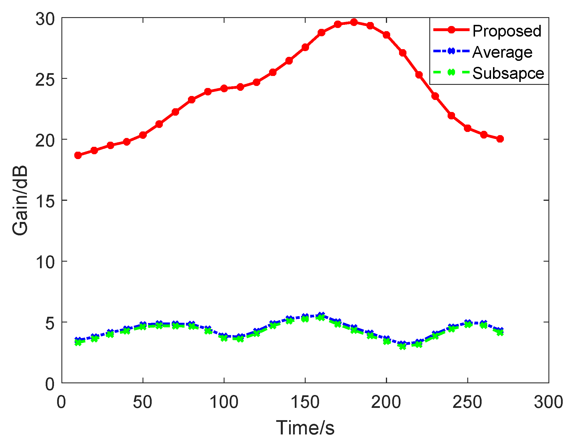
4.2. Experiments in Lake Trial Data

In this section, a set of lake trial data based on the distorted array is used to verify the effectiveness of the proposed method. In the experiment, the power amplifier as the acoustic source with 15 m in depth actively transmits the 83 Hz, 104 Hz, and 109 Hz low-frequency narrow-band signals and a chirp signal whose initial frequency is 90 Hz and bandwidth 8 Hz. The other ship equipped with a towing array of 64 hydrophone sensors with a uniform interval of $1.5$ m, located 1 km away, is used to acquire the radiated noise data. There is a slight bow in the array. The data duration of T is 300 second, and the sample rate is 4 kHz.

The three narrow-band frequencies of 83 Hz, 104 Hz, and 109 Hz are acquired by using the narrow-band frequency detection. The corresponding time-delay differences are shown in Figure 8a. It is observed that some perturbations of time-delay differences exist among these detected frequencies, and they would result in large derivations from each other and lead to the appearances of outliers. The possible reason is that the SINRs in each detected narrow-band frequencies are quite different. The time-delay differences estimation in the average method, the subspace-based method, and the proposed WORKS method are shown in Figure 8b, respectively. The time-delay differences in the proposed method are quite smooth and slowly change, compared to thees in the average method and the subspace method. The output time-frequency spectrum based on the enhanced signals during 300 s are given in Figure 9a–d. It is found that the spectrum of enhanced signals based on the proposed method has higher amplitudes in both narrow-band signals and chirp signals, compared to these in the other two methods. The proposed method is superior to the average operation and the subspace-based methods. The quantitative performance concerning the average gains of three narrow-band frequencies are provided as shown in Figure 10. Note that the gains are calculated by the narrow-band frequency amplitude in the output signal over that in the conventional beamforming assuming a hypothetical uniform linear array due to the unknown distorted array shape. It is found the gains in the our proposed method are generally above 15 dB, even up to 30 dB, compared to about 5 dB gains in both the average operation and the subspace-based methods.

5. Conclusions

A robust and data-driven signal enhancement scheme is proposed to take into account the array distortion in this paper. The proposed scheme firstly extracts the phases of narrow-band signals from the conventional beamforming result using narrow-band signal detection. Then, we proposed a novel weighted outlier-robust Kalman smoother to estimate time-delay differences to mitigate outliers in the time-delay differences. Finally, an enhanced output signal is achieved by beamforming based on the estimated time-delay differences. The proposed scheme is validated by both simulations and experiments. The proposed method is a data-driven approach that fully exploits the directional radiated noise signal due to distant underwater acoustic targets as sources of opportunity for real-time array shape estimation. It requires neither the number nor direction of sources to be known in advance.

References

1. Schurman, I. Reverberation rejection with a dual-line towed array. IEEE J. Ocean. Eng. 1996, 21, 193–204. [Google Scholar] [CrossRef]
2. Felisberto, P.; Jesus, S.M. Towed-array beamforming during ship’s maneuvering. Proc. Inst. Elect. Eng. Radar Sonar Navig. 1996, 143, 210–215. [Google Scholar] [CrossRef]
3. Park, H.Y.; Lee, C.; Kang, H.G.; Youn, D.H. Generalization of the subspace-based array shape estimations. IEEE J. Ocean. Eng. 2004, 29, 847–856. [Google Scholar] [CrossRef]
4. Hodgkiss, W. The effects of array shape perturbation on beamforming and passive ranging. IEEE J. Ocean. Eng. 1983, 8, 120–130. [Google Scholar] [CrossRef]
5. Groen, J.; Beerens, S.P.; Doisy, Y. Shape and Doppler correction for a towed sonar array. In Proceedings of the Oceans’04 MTS/IEEE Techno-Ocean ’04, Kobe, Japan, 9–12 November 2004; Volume 2, pp. 613–620. [Google Scholar]
6. Owsely, N.L. Shape estimation for a flexible underwater cable. IEEE EASCON 1981, 14, 16–19. [Google Scholar]
7. Gray, D.; Anderson, B.; Bitmead, R. Towed array shape estimation using Kalman filters-theoretical models. IEEE J. Ocean. Eng. 1993, 18, 543–556. [Google Scholar] [CrossRef]
8. Newhall, B.; Jenkins, J.; Dietz, J. Improved estimation of the shape of towed sonar arrays. In Proceedings of the IEEE Instrumentation and Measurement Technology Conference, Como, Italy, 18–20 May 2004; pp. 873–876. [Google Scholar]
9. Rockah, Y.; Schultheiss, P.M. Array shape calibration using sources in unknown locations—Part I: Far-field sources. IEEE Trans. Acoust. Speech Signal Process. 1987, 35, 286–299. [Google Scholar] [CrossRef] [Green Version]
10. Weiss, A.J.; Friedlander, B. Array shape calibration using sources in unknown locations-a maximum likelihood approach. IEEE Trans. Acoust. Speech Signal Process. 1989, 37, 1958–1966. [Google Scholar] [CrossRef]
11. Gray, D.A.; Wolf, W.O.; Riley, J.L. An eigenvector method for estimating the positions of the elements of an array of receivers. In Proceedings of the Conference Signal Processing Applic, Adelaide, Australia, 17–19 April 1989; pp. 391–393. [Google Scholar]
12. Smith, J.J.; Leung, Y.H.; Cantoni, A. Sptatistics of the phase delays between array receivers estimated from the eigendecomposition of the signal correlation matrix. In Proceedings of the Conference IEEE International Conference on Acoustics, Speech and Signal Processing, Adelaide, SA, Australia, 19–22 April 1994; pp. 325–329. [Google Scholar]
13. Bouvet, M. Beamforming of a distorted line array in the presence of uncertainties on the sensor positions. J. Acoust. Soc. Am. 1987, 81, 1833–1840. [Google Scholar] [CrossRef]
14. Owsley, N.L.; Swope, G.R. Array shape determination using time delay estimation procedures. IEEE EASCON 1980, 13, 158–164. [Google Scholar]
15. Odom, J.L.; Krolik, J.L. Passive towed array shape estimation using heading and acoustic data. IEEE J. Ocean. Eng. 2015, 40, 465–474. [Google Scholar] [CrossRef]
16. Ferguson, B.G. Sharpness applied to the adaptive beamforming of acoustic data from a towed array of unknown shape. J. Acoust. Soc. Am. 1990, 88, 2695–2701. [Google Scholar] [CrossRef]
17. Quinn, B.G.; Barrett, R.F.; Kootsookos, P.J.; Searle, S.J. The estimation of the shape of an array using a hidden Markov model. IEEE J. Ocean. Eng. 1993, 18, 557–564. [Google Scholar] [CrossRef] [Green Version]
18. Wahl, D.E. Towed array shape estimation using frequency wavenumber data. IEEE J. Ocean. Eng. 1993, 18, 582–590. [Google Scholar] [CrossRef]
19. Viberg, M.; Swindlehurst, A.L. A Bayesian approach to autocalibration for parametric array signal processing. IEEE Trans. Signal Process. 1994, 42, 3495–3507. [Google Scholar] [CrossRef] [Green Version]
20. Ross, D.; Kuperman, W.A. Mechanics of underwater noise. J. Acoust. Soc. Am. 1989, 86, 1626. [Google Scholar] [CrossRef]
21. Wales, S.C.; Heitmeyer, R.M. An ensemble source spectra model for merchant ship-radiated noise. J. Acoust. Soc. Am. 2002, 111, 1211–1231. [Google Scholar] [CrossRef] [PubMed]
22. Information on the Swellex96 Experiment Data. Available online: http://swellex96.ucsd.edu/ (accessed on 15 July 2020).
23. Wu, Q.; Xu, P.; Li, T.; Fang, S. Feature enhancement technique with distorted towed array in the underwater radiated noise. In Proceedings of the INTER-NOISE and NOISE-CON Congress and Conference Proceedings. Institute of Noise Control Engineering, Hong Kong, China, 27–30 August 2017; Volume 255, pp. 3824–3830. [Google Scholar]
24. Ting, J.; Evangelos, T.; Stefan, S. A Kalman filter for robust outlier detection. In Proceedings of the IEEE/RSJ International Conference on Intelligent Robots and Systems, San Diego, CA, USA, 29 October–2 November 2007; pp. 1514–1519. [Google Scholar]
25. Ting, J.; Evangelos, T.; Stefan, S. Learning an outlier-robust Kalman filter. In Proceedings of the European Conference on Machine Learning, Warsaw, Poland, 17–21 September 2007; pp. 748–756. [Google Scholar]
26. Dempster, A.; Laird, N.; Rubin, D. Maximum likelihood from incomplete data via the EM algorithm. J. R. Stat. Soc. Ser. B 1977, 39, 1–38. [Google Scholar]
27. Bishop, C.M. Pattern Recognition and Machine Learning; Springer: New York, NY, USA, 2006; pp. 423–517. [Google Scholar]
28. Šimandl, M.; Královec, J.; Tichavsky, P. Filtering, predictive, and smoothing Cramer–Rao bounds for discrete-time nonlinear dynamic systems. Automatica 2001, 37, 1703–1716. [Google Scholar] [CrossRef]
29. Tichavsky, P.; Muravchik, C.H.; Nehorai, A. Posterior Cramer–Rao bounds for discrete-time nonlinear filtering. IEEE Trans. Signal Process. 1998, 46, 1386–1396. [Google Scholar] [CrossRef] [Green Version]
Figure 1. An example of a distorted hydrophone array.
Remotesensing 13 01773 g001
Figure 2. Spectrum example of real radiated noise.
Remotesensing 13 01773 g002
Figure 3. Time-delay differences varying with narrow-band frequencies in real data case.
Remotesensing 13 01773 g003
Figure 4. Performance comparisons. (a) Beamforming result based on the hypothetical array. (b) Estimation of array shape. (c) Comparison of the estimates of time-delay differences. (d) Time-delay differences in these detected narrow-band signals. (e) Spectrum of the improved output signal.
Remotesensing 13 01773 g004
Figure 5. Estimated time-delay difference variances.
Remotesensing 13 01773 g005
Figure 6. Amplitude error versus bearings of the radiated noise source.
Remotesensing 13 01773 g006
Figure 7. Average amplitude errors versus SINR in narrow-band signals.
Remotesensing 13 01773 g007
Figure 8. Performance comparisons. (a) Time-delay differences in 4 detected narrow-band signals. (b) Comparisons of the estimates of time-delay differences.
Remotesensing 13 01773 g008
Figure 9. Performance comparisons of Short Time Fourier Transform using 20 s hamming window with a window shift of 10 s. (a) Proposed method. (b) Average method. (c) Subspace method. (d) CBF method.
Remotesensing 13 01773 g009
Figure 10. Gains of the detected narrow-band frequencies.
Remotesensing 13 01773 g010