1. Introduction
Autonomous vehicle (AV) technology has been a widely investigated and researched area during the last few years. Consequently, intense competition is developing at an accelerated pace, and enormous investments are being made by several companies like Waymo, Cruise, Argo AI, Aurora, etc. [
1]. In addition, major companies like General Motors, Ford, BMW, Tesla, Volvo, Nissan, Hyundai motor company, and Toyota have been working on self-driving cars for the past five years or so. The investments of billions of dollars tend to shape the future of AVs and unfolds the huge economic growth and social impact in the near future. AVs gather the data from a variety of sensors to guide the computer running an autonomous vehicle, legally qualified as the “driver” as per [
2]. The complete suite of sensing technologies in AVs includes cameras (both monochrome and color), radar, ultrasonic sensors, and light detection and ranging (LIDAR) [
3] that help the self-driving system (SDS) to drive autonomously. Cameras are traditionally used for sensing local environments like traffic signs, lane detection, etc. [
4]. Short-range radar and ultrasonic sensors serve the purpose of lane-change detection, blind-spot detection, parking assistance, etc., while long-range radar focuses on object detection, adaptive cruise control, localization, tracking, etc. [
5]. LIDAR is also used for object detection and classification, localization, collision avoidance, and emergency braking. In addition, short-range LIDAR detects and identifies various objects like pedestrians, sidewalks, other vehicles, etc. Although LIDAR performs poorly under bad weather conditions, its capacity to provide high spatial and longitudinal resolution makes it an effective and attractive technology for AVs.
Figure 1 shows the sensors equipped on an AV.
Perception system design is the central part of the development of AVs, which serves as the eyes and ears of the AVs. With the help of the large options for sensors and off-the-shelf schemes, the selection of appropriate sensors for perception systems has become very important. LIDAR is significantly important for AVs as it offers high-resolution 3D data of distant objects even at night with the absence of light. To provide a high-resolution 3D map of the surrounding environment, existing LIDAR lacks several important aspects. Similarly, 1D and 2D LIDAR do not provide dense point clouds, necessary for object detection, so they are not appropriate for environment perception. Predominantly, Velodyne’s rotating scanner HDL-64E is the most widely used LIDAR for AVs. It is equipped with a set of 64 laser diodes that work as a rotating block. The rotating laser block as a single unit is more effective than the rotating mirror technology. The resulting horizontal angular resolution is 0.4° with a 360° horizontal field of view (HFoV) and a 26.8° vertical field of view (VFoV) [
7,
8]. The moving part design of the Velodyne LIDAR and the complexity of its mechanical system make it expensive even when producing a large number of units [
3]. Although the upper and lower block of the Velodyne LIDAR collects the distance information simultaneously, only one laser from each block is fired at a time [
8]. Another drawback of pulse-scanning LIDAR like the Velodyne HDL-64E and SICK LMS511 is the maximum measurable range.
The goal of LIDAR is to get high-resolution 3D distance images with high refresh rates and long distances. The key performance indicators are the maximum range, range resolution, positional precision and accuracy, angular resolution, HFoV, VFoV, and frame refresh rate [
9,
10]. These indicators are mutually related; therefore, improving one parameter degrades the others. For higher angular resolution, a low refresh rate per second is required as the maximum measurable range is proportional to the maximum pulse repetition period. The idle listening time between pulse transmission and reception, particularly in pulsed-scanning LIDAR, is a significant obstacle in improving performance indicators simultaneously. Moreover, the idle listening time for reception increases with the increase in the maximum measurement range [
11,
12]. Another problem with current LIDAR is the range ambiguity for which a random pattern technique [
13,
14] and multiple repetition rates [
15] are introduced. It works on the correlation between the transmitted and received patterns, yet it is very difficult to discriminate between low-intensity reflected pulses in the presence of high-intensity return pulses.
To overcome the issues of the maximum detection range and higher resolution of LIDAR point clouds, this study proposed a pulsed-scanning LIDAR and made the following contributions
A pulsed-scanning LIDAR system is presented that works with concurrent emissions with body rotation. The concurrent operational mechanism overcomes the limitation of low resolution in traditional LIDARs such as Velodyne and SICK LMS series LIDARs and provides a long scanning range.
This LIDAR system can constantly measure distance with very little idle listening time within the pulse repetition period because its laser pulses include a unique identification number encoded by applying optical code division multiple access (OCDMA). Therefore, this system emits in each observation angle without waiting for a return pulse.
The proposed scanning LIDAR system solves the range ambiguity problem where the LIDAR cannot discriminate between the previous pulses and the current one, overlapping each other in the temporal domain.
A 2D pulse-coding scheme is utilized comprised of OCDMA and dense wavelength division multiple access (DWDMA) to formulate the pulse wavelength.
Extensive simulations were performed to evaluate the performance of the proposed LIDAR system. Results indicated that the proposed LIDAR system had better performance than commercial LIDAR systems in every aspect.
The rest of the paper is organized in the following manner. Important research works that are closely linked with the current study are discussed in
Section 2. The architecture of the proposed LIDAR system and its working mechanism are presented in
Section 3.
Section 4 describes the experiment setup, results, and analysis of the results. In the end, the conclusion and future works are given in
Section 5.
2. Related Work
During recent years, wide research efforts have been put forward for AVs comprising sensing technologies, efficient energy solutions, and effective driving operation control tools and strategies. For sensing technologies, LIDAR (2D and 3D solutions) and cameras (color, thermal, hyperspectral) have been investigated. Consequently, a large body of works on these sensors, as well as sensing approaches exists in the literature. This section discusses those related works that focus on LIDAR systems and their sensing strategies for AVs including the design of the LIDARs and the limitations of existing LIDAR products available for AVs.
2.1. Time-of-Flight Principle
The basic principle of LIDAR operation involves launching a pulse and detecting it by a sensor when it is reflected by the target [
11,
12].
Figure 2 shows the general working principle of the LIDAR. The distance is calculated by measuring the round trip time, and this principle is called the time-of-flight (ToF).
The maximum range and resolution of the LIDAR are determined by several parameters like the wavelength of waves, beam divergence, and scattering when the beam propagates through a given medium. The equations for measuring the range (
R), maximum range (
), and range resolution (
) are given as:
where
c represents the speed of light,
is the ToF,
W is the pulse width, and
is the pulse repetition frequency. The three most widely used wavelengths for LIDAR, especially automotive LIDAR, are 905 nm, 940 nm, and 1550 nm. Each of these wavelengths has its pros and cons as absorption is caused by water vapor in the upper atmosphere and rain and fog. The total reflected laser power received at the detector is given by:
where
represents the received laser power,
is the transmitted laser power,
shows the reflectance of the target area,
d is the length of one side of the projected area on the target,
refers to the illuminated area,
is the area of the receiver,
R is the range,
is the transmission efficiency through the atmosphere, and
is the receiver system optical efficiency [
12]. We looked at the operation and characteristics of the LIDAR from four perspectives: scanning LIDAR with a simple pulse, flash LIDAR, frequency-modulated continuous-wave (FMCW) LIDAR, and scanning LIDAR with coded pulses.
2.2. Scanning LIDAR with a Simple Pulse
Scanning LIDAR constructs a 3D point cloud using the distance between the LIDAR and the object. Distance is obtained using the round trip travel time from the laser to the target. The point cloud is constructed using one point at a time or one line of points at a time; the former is called single-laser LIDAR, while the latter is a multiple-laser LIDAR.
Figure 3 shows the operating procedure of SICK LMS511, which is a single-laser LIDAR.
Among the most widely used scanning LIDARs for AVs is the Velodyne HDL-64E spinning LIDAR. Although Velodyne has various models for 16, 32, 64, and 128 channels, the HDL-64E with the 64 channel model is the most common choice for autonomous vehicles. Equipped with 64 stacked laser-detector pairs, it scans simultaneously with a vertical range of 26.9° and a 0.4° horizontal angular resolution. The laser sources are placed 905 nm in two separate blocks that spin at 360° providing a range of 120
. Besides Velodyne, Luminar also produces a LIDAR based on moving part technology, which is expensive even when produced in large volumes.
Figure 3 is adaptable to the working mechanism of the Velodyne HDL-64E model. The 64 laser diodes of the HDL-64E are divided into two groups. Two groups have 32 laser diodes each and fire a laser in their own sequences. The LIDAR fires a laser pulse from a group to a target, and then, it waits for the reflection of the laser. After the reception, it calculates the target distance using the ToF principle. It repeats these sequences for laser diodes in a group. Once firing all diodes has finished, the LIDAR rotates the body to the next angle and restarts.
The second type of scanning LIDAR uses a non-moving parts technique involving the use of microelectromechanical systems (MEMS) scanning mirrors. Such a LIDAR system is robust for different harsh mechanical and temperature environments due to the small scanning mirrors, inertia, and resonant frequency. Three-dimensional scans from such a LIDAR require fractions of a second and provide a real-time solution for autonomous vehicles. However, the MEMS mirror LIDAR has the limitation of a smaller angular field of view, and a single unit cannot provide a full 360° view.
An alternative scanning scheme to MEMS-based beam scanning was provided in [
16] to accomplish low-cost and high-speed 3D sensing. Contrary to using the beam scan or 2D photo imaging, a combination of position-to-angle lenses is used with wavelength division multiplexing/demultiplexing (WDM). Experiments were conducted using four WDM channels with the ToF distance measurement approach to show that the angular resolution of the beam array can be improved by dithering the fiber arrays. Results demonstrated that the proposed scheme is especially attractive for LIDAR systems.
2.3. Flash LIDAR
Contrary to the scanning LIDAR, the flash LIDAR follows the no moving parts mechanism and operates as flash cameras do. Unlike the point-to-point construction of the point cloud in the scanning LIDAR, the flash LIDAR constructs the point cloud either one horizontal place at a time or the entire 3D point cloud in a flash [
3]. It thus overcomes the limitation related to the time for scanning technology. The field of view depends on the area illuminated by the detector, which contains an array of avalanche photodiodes (APDs) called the focal plane array (FPA) [
17]. Each element in the detector estimates the distance following the ToF principle, so the resolution of the flash LIDAR depends on the number of APDs in a detector FPA. There is a trade-off between the resolution and number of photons (signal-to-noise ratio (SNR)), where reducing the pixel size increases the resolution, but reduces the SNR and vice versa [
3]. Traditionally, the range of flash LIDAR is less, and it covers a few tens of meters. Recently released flagship smartphones have lower power and short-range variants of flash LIDAR to improve photos and support the augmented reality (AR) environment [
18].
Figure 4 shows the working principle of the ASC Peregrine, which is a flash LIDAR system.
2.4. Frequency-Modulated Continuous-Wave LIDAR
FMCW LIDAR is a complex LIDAR that offers both the distance and velocity of the detected object. It follows the principle of FMCW radar, where radio waves are continuously emitted using up chirp and down chirp mechanisms. Distance is then determined using the round trip time, while the velocity using the Doppler shift [
19]. For FMCW LIDAR, both a tunable laser, as well as a fixed-wavelength laser with a chirp modulator are used. A photodetector is used for detecting the modulated returned light to recover the modulated frequency, which is later used to estimate the range and velocity by mixing it with the frequency of the local oscillator [
3], as illuminated in
Figure 5. FMCW LIDAR provides tolerance to ambient light and offers both distance and velocity. Unlike the scanning LIDAR that uses a 950 nm laser, FMCW LIDAR uses narrow-linewidth long coherent 1550 nm lasers [
20].
A LIDAR scheme called “swept-source LIDAR” was presented in [
21] that uses the FMCW ranging with an optical phased array (OPA) that has no moving parts. OPA LIDAR contains several optical elements that act as antennas to re-emit the coherent light. The direction is controlled by the phase and amplitude of the re-emitted light and can be steered in any direction. The authors designed a real-time LIDAR with a
MHz update rate in [
22] that uses dispersive Fourier transformation and the instantaneous microwave frequency. The femtosecond laser pulse goes through an all-fiber Mach–Zehnder interferometer, and the displacement is encoded into the frequency variation of the temporal interferogram. The real-time challenges of storage and processing are dealt with using microwave photonic signal processing. Experiments were conducted with an adjustable dynamic range by using a programmable optical filter. Results indicated that the proposed system could achieve a standard deviation of
and a mean error of
over the 15
detection range. To overcome the limitation of pulse energy decreasing from increased laser repetition rates, an 885 nm laser diode-based LIDAR system was proposed in [
23]. Using a master oscillator power amplifier (MOPA), the
mJ,
ns 1064 nm pulses were obtained at 2 kHz. The system aimed at achieving high energy to accomplish high-resolution range imaging for long distances. Results demonstrated that 1064 nm and 1532 nm pulses were suitable for avalanche photodiode array LIDAR and streak tube imaging LIDAR. The proposed system showed high stability for a temperature range of −10° to 30° and a vibration frequency of 10 Hz to 100 Hz. Similarly, an FMCW LIDAR system was proposed in [
24] that aimed to reduce the hardware complexity and post-processing to improve the distance resolution. The higher beat frequency of FMCW LIDAR was reduced using digital down-convert (DDC) technology, and the fast Fourier transform (FFT) was extracted at 256 points, which were 25 times smaller than the existing 8192 points. Experiments showed that the performance of a
root mean squared error (RMSE) was improved as compared to the conventional approach. Compared to the scanning LIDAR systems, this solid-state beam steering offers robustness for LIDAR systems. Although in its infancy, it offers promising capabilities for automotive LIDAR.
2.5. Scanning LIDAR with Coded Pulses
Figure 6 shows the functional diagram of the proposed LIDAR scanning system with coded pulses. The red color in the figure corresponds to the transmission operations, while the cyan color is the part that performs the reception operations.
The authors presented a LIDAR system based on direct-sequence OCDMA (DS-OCDMA) that uses the coded pixel location information in its laser pulses [
25]. OCDMA is a multiple access technology by which each communication channel is distinguished by a specific optical code rather than a wavelength or time-slot. An encoding operation optically transforms each data bit before the transmission. At the receiver, the reverse operation is performed to decode the received data to recover the original data. The encoding and decoding operations alone constitute optical coding. Additionally, a scanning-based MEMS mirror was used with DS-OCMDA to overcome the idle listening time limitation of conventional LIDAR systems. The idle time was removed because the added laser pulses carried the pixel location information, which was encoded using DS-OCDMA. The pulses were fired in each direction without the time delay required to receive the fired pulses in conventional LIDAR systems. To receive the reflected pulses, an indium gallium arsenide photoconductive antenna (InGaAs PCA) was used while the demodulation was done using a time-to-digital converter (TDC) and DS-OCDMA. The sequential firing LIDAR scanner used a 905 nm laser pulse with a very short width of less than
ps and a MEMS mirror that scanned an 848 × 480 resolution, 60 times per second [
26]. Simulation results suggested that the proposed LIDAR had better performance than the Velodyne HDL-64E and ACS Peregrine LIDAR systems.
The performance of the proposed LIDAR system in [
25] was evaluated by a prototype [
10] manufactured using commercial parts. For this purpose, intensity-modulated direct detection OCDMA was used with non-return-to-zero on-off keying to remove the idle time. The laser pulse used in the prototype was 5 ns, and the MEMS mirror could move 1000 times per second. With respect to measuring the distance to the destination, it was possible to measure once per second at a resolution of 30 × 30. Although the desired measurement speed was not obtained in the prototype, the validity of the operation of the coded pulse method was determined efficiently. A series of pulses was used in the system, and alien pulses were removed using several decision steps. The built prototype was tested on shot and background noise, and results showed that the proposed system could eliminate both noises.
The transmitted signal strength and SNR mainly determine the maximum measurable distance of the LIDAR. Both items are related to the received signal strength, but their approaches are different. Using the transmitted laser power is a method of increasing the reflected laser pulse power by using a laser pulse with the maximum power allowed by the acceptable exposure limit (AEL) and measuring it at a distance as far as possible. Using the SNR is a method of measuring a long distance using even a small reflected pulse by setting the threshold value determined by the reflected and received laser pulse power as low as possible. The coded pulse scheme has several potential differences from that of the conventional scanning approach. The traditional LIDAR measures the distance using only one pulse, but this LIDAR using the encoding code has advantages. Using multiple pulses instead of one pulse for a single destination reduces the maximum power that can be assigned to a single pulse to comply with the AEL Class 1. When the distance is measured in the same way as the conventional LIDAR without a coded pulse, if the maximum power decreases, the maximum measurement distance also decreases due to attenuation caused by the distance, as shown in Equation (
4). On the contrary, using the encoding code, since several pulses are reflected and returned from one measuring point, the distance measurement is possible using all the received pulses. Since there is a specific pattern using multiple pulses, it is possible to measure a long distance by applying the SNR as low as possible, which improves both precision and accuracy. The maximum reception distance of the LIDAR refers to the maximum distance for which the received signal strength can be distinguished from noise. After the pulse is reflected from the destination, the received signal strength is inversely proportional to the square of the distance to the destination. A strong signal is received when the distance to the destination is close, and a weak signal is received as the distance is increased. For this reason, when a large SNR is used, the received signal is clearly distinguished from noise and the false alarm rate very low, but the measurement distance is shortened due to the need for a high received signal strength. If a low SNR is used, the false alarm rate is high because the received signal is difficult to distinguish from noise, but a low received signal strength is required, so the range of the maximum distance increases. In the case of LIDAR or radar, a large SNR is preferred because a low false alarm rate is important, and a high received signal strength is used. Each of the received signals is difficult to distinguish from noise, but when multiple pulses are used, it is possible to determine whether they have the same pattern as the transmitted signal by analyzing the pattern. Even if the power of a single pulse is distributed and transmitted, the transmission signal can be detected using a low SNR, so it is possible to measure a similar or distant place compared to the method using a single pulse.
Since the distance to the destination is calculated by the time difference between the transmitted coded pulses and the received coded pulses, it is necessary to accurately measure the time interval between the transmitting pulse and the receiving pulse for accurate distance calculation. The time of the transmission pulse always has the same error as the time transmitted from the LIDAR is used. For the pulse of the received signal, a relatively large error occurs due to the channel environment or the physical reflection characteristics of the reflected point involving the transmission and reception of the laser pulse. A general LIDAR uses a Gaussian pulse, and the shape of the received pulse has a shape in which the Gaussian pulse is very broken due to the influence of noise in the channel environment and reflection characteristics; this shape changes each time it is received. Even if various methods of inferring the original Gaussian shape of the pulse and the center of the damaged pulse by noise are used, the original shape cannot be restored efficiently. The standard for measuring the distance in the received signal is based on the center point of the Gaussian pulse, and the accuracy of the distance is also affected by the error generated by the shape of the pulse, so the accuracy is lowered. In the case of using multiple pulses, even if individual pulses are affected by noise and there is a difference from the transmitted pulse type, if the average of the multiple pulses is taken, these errors can also be reduced.
In this LIDAR scanner, accuracy and precision were improved by 37% and 85%, respectively, with greater distances using the proposed OCDMA-based system. The OCDMA ToF LIDAR determines the maximum distance, accuracy, and precision according to the number of pulses used. It is necessary to select an appropriate coding method according to the purpose of using the LIDAR [
10,
27].
A 2D OCDMA modulation was proposed in [
28] that utilizes wavelength-hopping time-spreading codes for LIDAR. Synopsys RSoft OptSim simulation software was used to implement the proposed approach using carrier-hoping prime codes (CHPC). Results demonstrated that OCDMA ToF LIDAR is flexible for adopting various code parameters and supports concurrent ToF measurements more than the 2D LIDAR.
We summarize the characteristics of related works in
Table 1.
3. Proposed LIDAR Scanner System Using Concurrent Firing Coded Pulses
Despite the discussion of the above related works from the literature, high-resolution with long-range LIDAR at a high refresh rate remains an open research area and requires dedicated research efforts. This research aimed to utilize a concurrent firing mechanism using the body rotation approach to overcome this limitation.
3.1. Operation and Limitation of Previous Works
A 3D LIDAR uses the azimuth angle and elevation angle of the spherical coordinate system to identify the target point for measuring its distance. As described in
Section 2.5, a LIDAR scanner that sequentially measures the distance to a destination using an encoded pulse was proposed [
25]. In this sequential firing LIDAR scanner, the azimuth angle and the elevation angle were not separately distinguished, and the target point information was used to represent the coded laser pulse based on the asynchronous prime sequence code. That is, after generating and transmitting encoded laser pulses for one target point, the MEMS mirror angle was adjusted to the next target point without waiting for the reception of the reflected wave [
10]. Then, a new encoding pulse for the target point was generated, and the laser pulse was transmitted. When the received laser pulse was decoded, the target point information could be known, and the moving time and distance of the laser pulse could be calculated accordingly.
The previously proposed sequential firing LIDAR scanner maintained the advantages of the maximum measurable distance and improved measurement accuracy [
27]. These advantages were obtained using multiple pulses with MEMS mirrors with a width of tens to hundreds of picoseconds. Previously, a sequential scanning method was proposed that used an OCDMA method based on an asynchronous prime sequence code to support multiplexing. Multiplexing support means sending multiple pulses to measure the distance of another target point before the distance measurement of one target point is finished, i.e., before receiving the reflected pulses from that measurement point. It is a method of measuring distances to multiple target points at the same time because even if a pulse reflected from several places is received at the same time, information about the target point can be grasped by decoding the encoded content. On the other hand, in the conventional simple pulse method, when several pulses are received, it is not possible to distinguish which pulse is reflected from which target point exactly. Since it is possible to measure only one target point at a time, the measurement time is constant according to the maximum measurement distance, so even if a laser pulse sent to the target point is received, the distance to the next target point is measured after the predetermined measurement time has passed.
The asynchronous prime sequence code is a method of encoding using a prime number larger than the number of multiplexing, and one bit is encoded as a chip of the square of the prime number. This code used by the sequential firing LIDAR scanner was a coding method that used the presence or absence of laser pulses. However, not all chips have pulses, but because there is one pulse for each prime number, the resulting number of pulses for encoding one bit was the same as the prime number. The cardinality representing the maximum number of multiplexing was only the prime number, and the number of chips required was proportional to the square of the prime number. Therefore, for high cardinality, a prime number equal to or greater than the cardinality must be used. Since the number of chips required when encoding 1 bit is the square of the prime number, 1 bit was converted into a row of chips having a very long length. For example, if the number of multiplexing is 10, encoding using 121 chips is the square of 11, which is a prime number greater than 10. If five bits are encoded, the information is increased to 605 chips, of which the number of pulses is 55. As the stream of the chip increases, the time required for the transmission increases proportionally, so the time required to transmit all laser pulses increases in proportion to the product of the square of the prime number and the number of bits. Since the angle can be moved to another target point only when all the chips to be transmitted to the target point are finished, the time to stay at one measurement angle increases, and the time required for one rotation increases accordingly.
Since the diameter of the laser pulse reflected by the mirror is proportional to the cosine of the angle of incidence, the diameter of the pulse increases when the angle of incidence is close to a right angle. In addition, the method of using a mirror is susceptible to vibration, so accuracy decreases when it is mounted on a moving object. Similarly, the MEMS mirror method has a small moving angle range and moving unit, and its speed is low, making it impossible to quickly measure a large area.
3.2. Enhanced Methodology of Concurrent Firing Coded Pulse
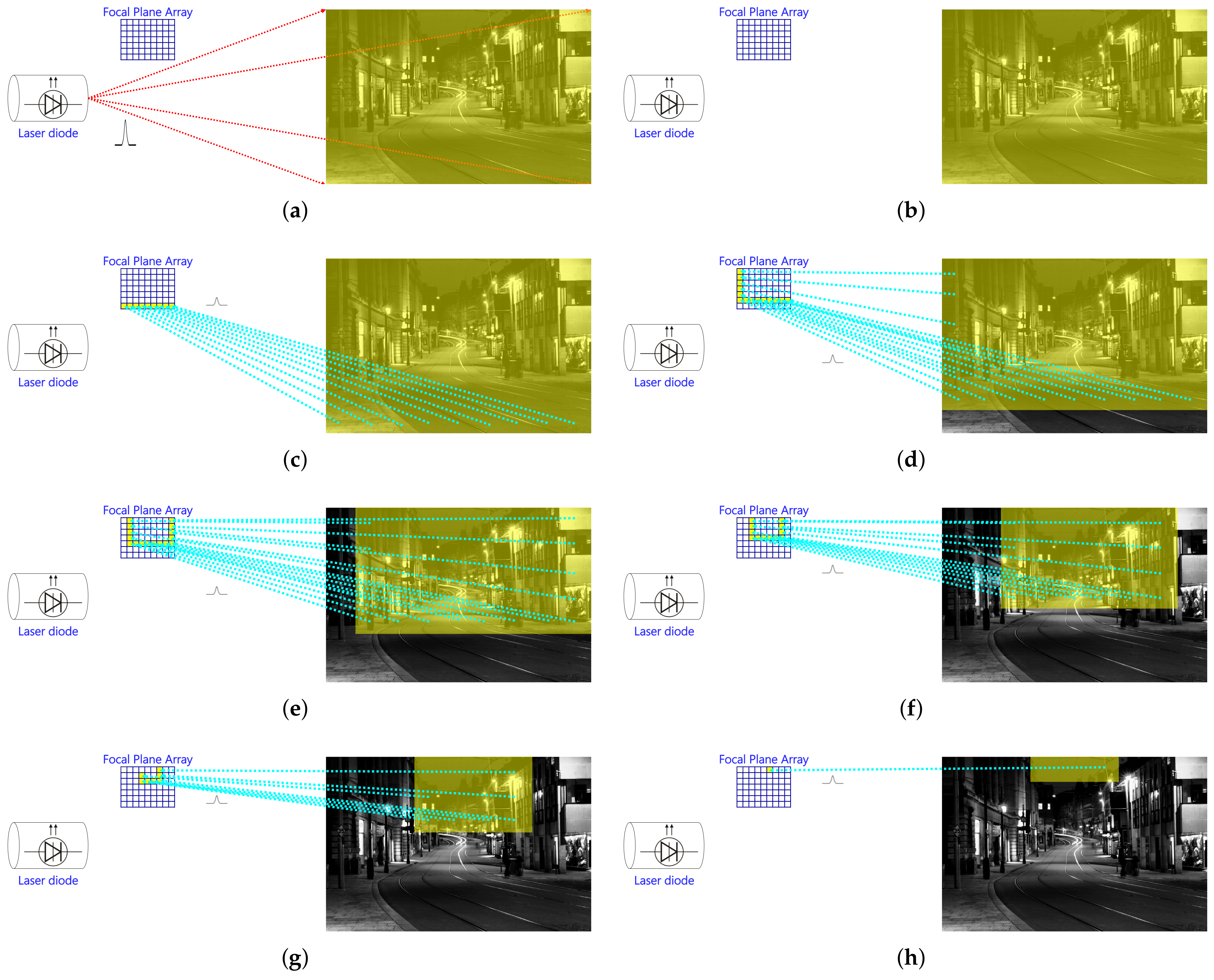
The proposed concurrent firing LIDAR scanner used several methods to overcome the limitation of the sequential firing LIDAR scanner while using the advantages of the encoded pulse. For sending laser pulses in the desired direction, the sequential firing LIDAR scanner used the reflection of the MEMS mirror, but the concurrent firing LIDAR scanner directly rotated the LIDAR body with laser sources attached to the body. In the sequential firing LIDAR scanner, the incidence angle and the reflection angle changed according to the target direction, which was measured by reflecting the laser in the desired direction using a mirror. As a result, the received signal strength varied even at the same distance.
The structure of the concurrent firing LIDAR is shown in
Figure 7. The proposed LIDAR scanner had the same structure as Velodyne’s VLS-128 where 128 laser sources were attached to the LIDAR body vertically, and the LIDAR body rotated slightly and measured the distance to 360°. The diameter of the pulse was similar to the original pulse diameter when the angle of incidence was close to 0°. The proposed LIDAR scanner had an azimuth angle of 360° according to the measurement interval, and 128 laser sources were mounted vertically to measure the elevation angle in each azimuth. The 128 elevation angles were divided by the wavelength of the laser source, and the azimuth angle used the encoded laser pulse based on the CHPC. When the body rotated to measure the azimuth, the same encoded pulse was generated from 128 laser sources using the azimuth information, and laser pulses of different wavelengths were transmitted according to the elevation angles. The elevation angle information could be known by the wavelength of the received laser pulse, and the azimuth angle information could be obtained by decoding the received pulse so that the laser pulse movement time and distance to the target point could be calculated. We selected an ADC12J4000 from Texas Instruments (TI), which is a 12 bit, 4 GHz radio frequency-sampling ADC. The accuracy or drift of time measuring depends mainly on the ADC, and ADC12J4000 has 0.1 ps RMS as the ADC jitter or 0.03 mm in distance. For complete details of the components used in the simulation, readers are referred to [
10].
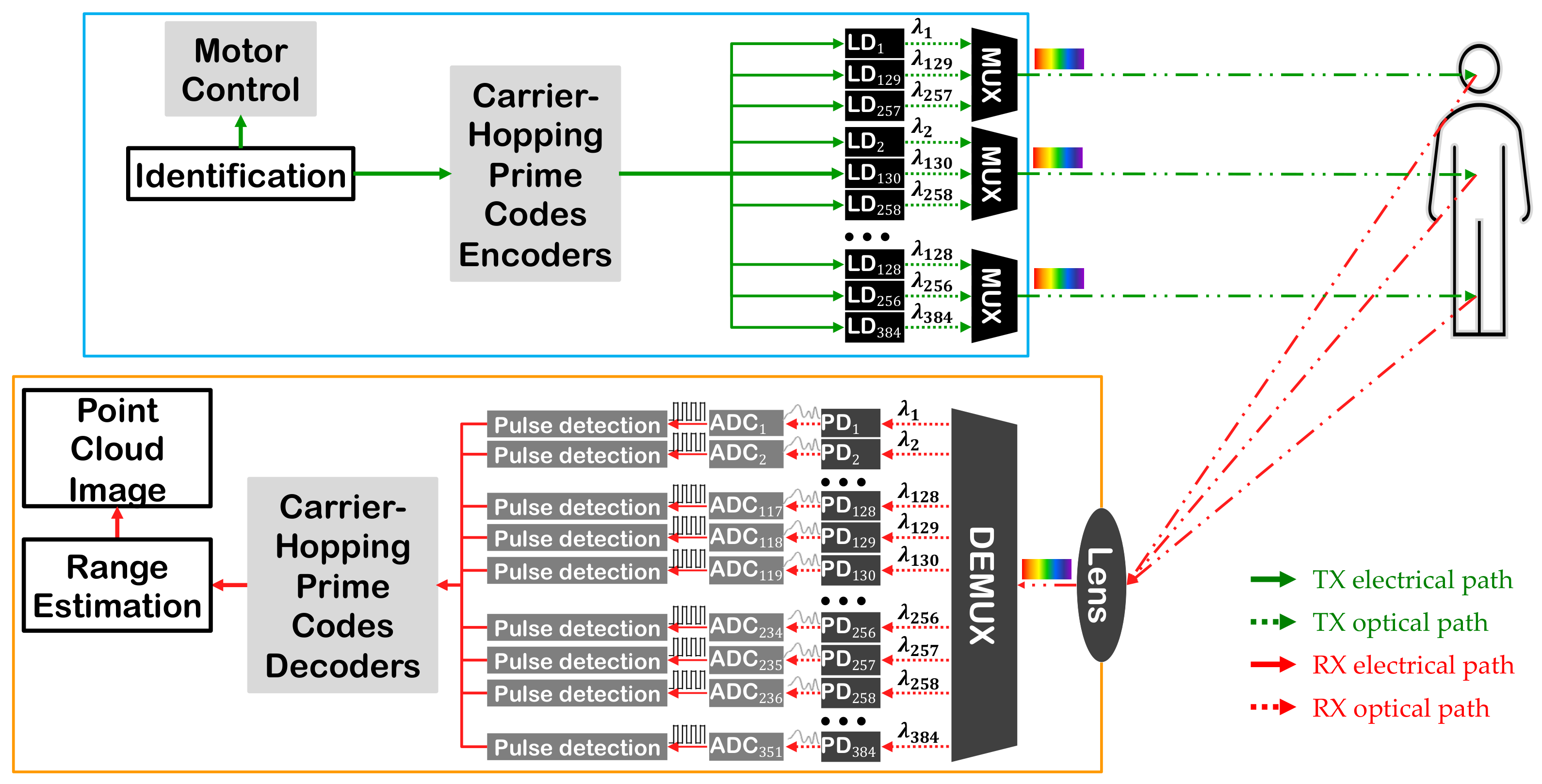
The transmitter rotated according to the desired azimuth as given by the azimuth information. Information for identifying the azimuth angle was encoded using a CHPC, and each of the 128 sources generated encoded laser pulses using three laser diodes (LDs) with different wavelengths. The green color in the figure corresponds to the transmission operations, while the red color is the part that performs the reception operations. The solid line is the path through which the electrical signal is transmitted, and the dotted line is the path through which the laser signal is transmitted.
The current time was recorded while transmitting a laser at an elevation angle corresponding to each source through one transmitter using the multiplexer (MUX) in each source. The laser pulses moved towards the target point at the speed of light, and when reflected from the object, they entered the LIDAR receiver through the lens. After being classified according to the wavelength of the reflected wave through the demultiplexer (DEMUX) in the receiver, it was converted into an analog electric signal using a photodiode that processed the wavelength. After converting to digital data using ADC, the pulse was detected by the sliding correlation method, and the original identification information was decoded by using the CHPC method. The time when the transmission was started was determined with the decoded identification information. The ToF was calculated, and the distance to the object was measured and added to the point cloud image. The operating strategy of concurrent firing LIDAR scanner with coded pulses is shown in
Figure 8.
The frequency used for the CHPC method in the concurrent firing LIDAR scanner was as follows. Vertically attached 128 laser sources required a total of 384 frequencies using 3 LDs to generate pulses of three different wavelengths. A total of 384 frequencies with
GHz intervals from
THz to
THz were allocated, as shown in
Table 2 below, mainly with the conventional band (C-band) defined for dense wavelength division multiplexing (DWDM) in ITU-T G.692 [
29,
30]. The
GHz center frequency intervals were spaced so that the wavelength difference of the laser pulses generated by the same source was large.
On the other hand, the CHPC used by the concurrent firing LIDAR scanner used several laser wavelengths. This is a coding method that can be identified according to the chip where the laser pulse is located at each wavelength.
Figure 9 expresses a CHPC with three wavelengths and 11 chips and a cardinality of 11. Although using a large number of wavelengths reduced the transmission time, it required the same number of laser pulses as that of the number of wavelengths. Reducing the power of every laser pulse to satisfy eye safety is difficult. In this study, priority was given to the maximum measurable distance of LIDAR, so only three wavelengths were used. The asynchronous prime sequence code used one wavelength and required 121 chips of 11 × 11 for cardinality 11; however, CHPC used three wavelengths, but only 11 chips were needed for each wavelength to transmit the pulses. Consequently, the time was reduced to a ratio of the square root, so the pulse was sent to the destination within a much shorter time. When using a pulse with a width of 5 ns, which is widely used in LIDAR systems, only 55 ns were required to transmit all the encoded pulses at one measurement angle. Therefore, it was possible to measure 360° very quickly while using a very narrow measurement angle. CHPC were generated using the following method. Given a set of
k prime numbers
binary (0,1) matrices,
, with ordered pairs [
29,
33]:
for the CHPC with cardinality
wavelength, length
and weight
where “
” shows a module
multiplication for
[
33].
4. Simulation Results and Discussion
This section discusses the simulation results of the proposed LIDAR system and compares its performance with other LIDAR systems.
4.1. Simulation Setup
For the performance evaluation of the proposed LIDAR scanner, two other state-of-the-art LIDAR scanners were selected including a sequential firing LIDAR scanner and the Velodyne VLS-128. The sequential firing LIDAR scanner was our previously proposed scanner [
10], while the VLS-128 is the state-of-the-art LIDAR from Velodyne. The VLS-128 uses 128 infrared (IR) laser pairs with IR detectors for measuring the distance to the objects. The mounted body spins around its axis to scan a 360° environment, with each laser fired 18,500 times per second to produce a rich and large 3D point cloud [
34]. It provides the highest resolution with the widest FoV in the world [
35]. Both, the sequential LIDAR and VLS-128 LIDAR scanners were selected due to their specifications, which were very similar to the proposed LIDAR scanner. For illustration, a comparison is provided in
Table 3.
The sequential firing LIDAR measured the destination once per second with 30 azimuth and 30 elevation angles, and the concurrent firing LIDAR measured the destination 25 times per second with 20,000 azimuth and 128 elevation angles, while the VLS-128 measured the destination five times per second with 3600 azimuth and 128 elevation angles. In order to compare the performance and strengths and weaknesses of these LIDARs, the width of the laser pulses used by the three LIDARs was equal to 5 ns. The sequential firing LIDAR scanner and the concurrent firing LIDAR scanner determined the length of information used for encoding. The same was done with nine bits, and the concurrent firing LIDAR scanner and the VLS-128 had the same FoV.
LIDARs used in automobiles generally comply with AEL Level 1, and the laser output is determined by the wavelength, pulse width, and the number of pulses of the laser used. The sequential firing LIDAR scanner uses a laser of a 903 nm band, and the number of chips it generates to send to one destination is 1089, of which 99 pulses are transmitted. Therefore, nine-hundred target points are measured per second, and 89,100 pulses are emitted per second, with 99 pulses corresponding to the AEL standard aperture. On the other hand, the concurrent firing LIDAR scanner used a laser of a 1550 nm band, and the number of chips generated to send to one destination was 297, of which the transmitted pulses were 27. As a result, there were 64,000,000 target points measured in 1 s, and the total number of pulses emitted in 1 s was 1,728,000,000. Among them, one-thousand three-hundred fifty pulses reached the AEL standard aperture. The VLS-128 uses a 905 nm laser and measures the distance using one laser pulse to one destination. Therefore, there were 2,304,000 target points measured per second, and the number of pulses emitted per second was 2,304,000, which reached the AEL standard aperture. The larger the number of laser pulses reaching the AEL standard aperture, the lower the power of the laser pulse should be.
Table 4 shows a simple comparison of representative LIDARs: SICK LMS511, Velodyne HDL-64E and VLS-128, ASC GSFL-4K, Luminar Hydra, the previously proposed sequential firing LIDAR scanner, and the currently proposed concurrent firing LIDAR scanner [
8,
9,
10,
25,
27,
34,
36,
37,
38].
Of the three LIDARs, the laser pulses emitted from the concurrent firing LIDAR scanner arrived at the aperture most frequently, and the VLS-128 arrived the least. By simply comparing the number of pulses, the VLS-128 could use the highest laser power, and the concurrent firing LIDAR scanner used the lowest laser power to comply with Class 1 of AEL. The sequential firing LIDAR scanner and VLS-128 use a laser in the near-infrared band near 903 nm, which adversely affects the human retina, but the concurrent firing LIDAR scanner used a laser in the mid-decimal band of 1550 nm band, which is less harmful to the human retina. For this reason, the highest laser power can be used even though the number of pulses of the concurrent firing LIDAR scanner was the largest among the three types of LIDARs.
To measure the performance of the proposed LIDAR scanner and compare the distance measurement performance with other LIDAR scanners, the environment shown in the
Figure 10 was configured for the simulation. A white paper wall and a black matte paper wall of 2
each in width and height were placed at a distance of
in front of the LIDAR, and the distance measurement was carried out according to the operation of the LIDAR described in the previous section. The reflectance of the white paper wall was 90%, and that of the black matter paper wall was 10%. For optical characteristics related to laser transmission/reception, reflection, lens, etc., Synopsys OptSim optical simulation software was used [
10,
39]. In addition, MATLAB was used for encoding and decoding, signal processing, and distance calculation tasks.
4.2. Performance Evaluation of the Proposed LIDAR Scanner
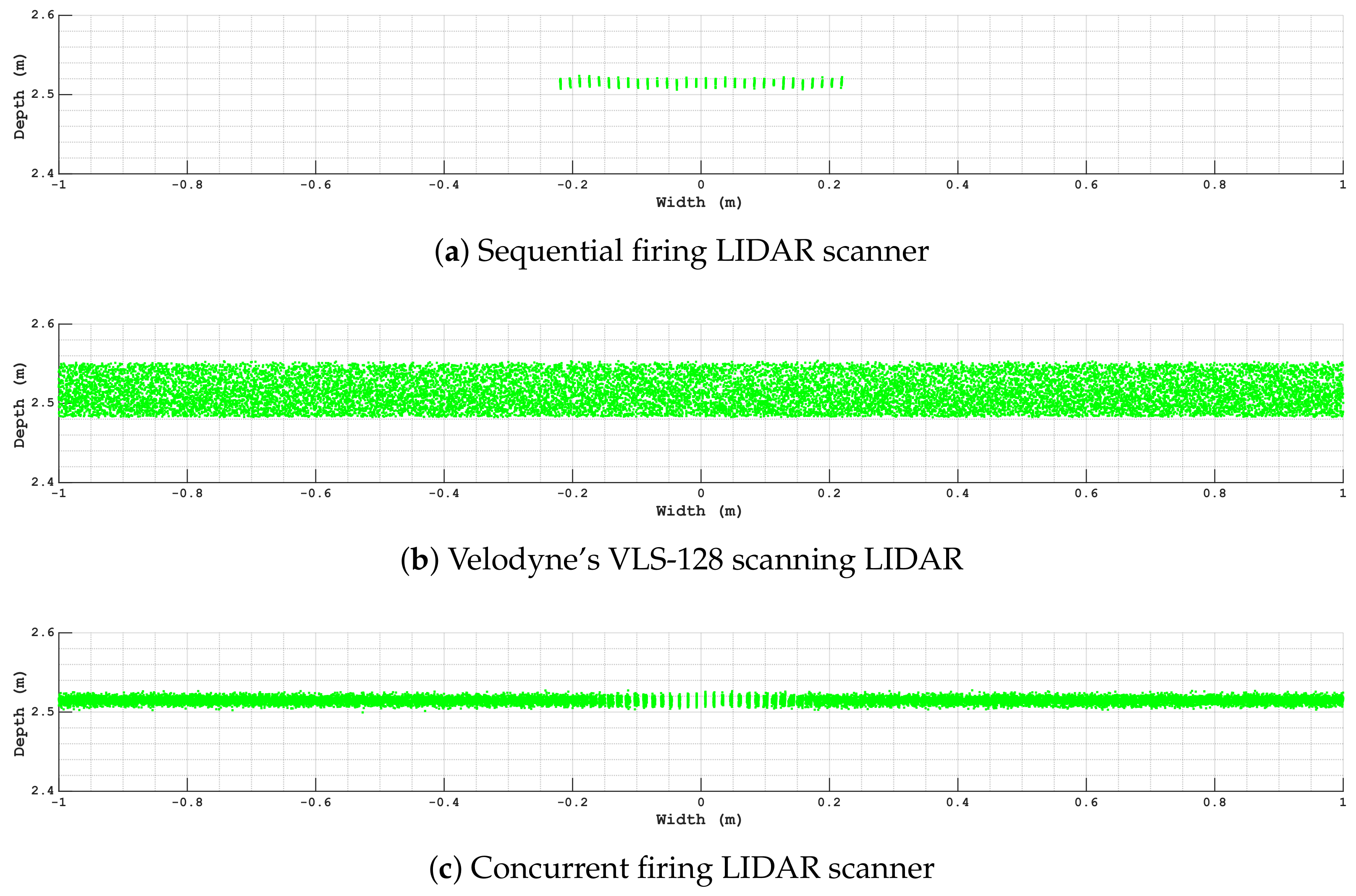
Simulation results indicated that the proposed concurrent firing LIDAR scanner had the widest FoV and the best angular resolution. Consequently, the number of locations where paper walls were measured was the largest for the proposed LIDAR scanner. The sequential firing LIDAR scanner had a poor FoV and angular resolution, so the paper wall measurement result was also the worst.
Figure 11a,b shows the location data measured by the sequential LIDAR scanners and the VLS-128 LIDAR scanner, respectively. Point cloud results from the sequential firing LIDAR were poorer than the VLS-128. The 3D point cloud generated using the proposed LIDAR is shown in
Figure 12. Results indicated that the 3D point cloud generated by the proposed concurrent firing LIDAR was rich as compared to both the sequential firing LIDAR and Velodyne VLS-128.
For further comparison of the three LIDAR scanners,
Table 5 is provided, which summarizes the properties of the LIDAR scanners. RSSI in
Table 5 indicates the received signal strength indicator of the pulse. The measurement result of the concurrent firing LIDAR scanner was the best, and the measurement result of the sequential firing LIDAR scanner was the worst. The proposed concurrent firing LIDAR scanner and the VLS-128 had the same FoV, but the number of measurements was very different due to the difference in angular resolution. VLS-128 had a non-linear distribution of angular resolution in elevation.
Figure 13 shows the locations measured by the paper walls in the three types of LIDAR in a top view format. These figures show the FoV and distance information of the azimuth angle for the measurement locations together. The FoV was determined by the unique specifications of each LIDAR method, but the distance information represented an error that occurred when measuring the distance. According to the central limit theorem, the more data are used to calculate, the less the error will be and the better the accuracy and precision. The sequential firing LIDAR scanner, which used the most laser pulses, had the least error, as shown in
Figure 13a. On the other hand, the VLS-128, which uses only one laser pulse, had the largest error, as given in
Figure 13b. Although the proposed concurrent firing LIDAR scanner used fewer laser pulses than the sequential firing LIDAR scanner, there was not much difference in the distance error. Thus, the proposed LIDAR scanner exhibited precision and accuracy, very similar to the sequential firing LIDAR, even when a lower number of laser pulses were used.
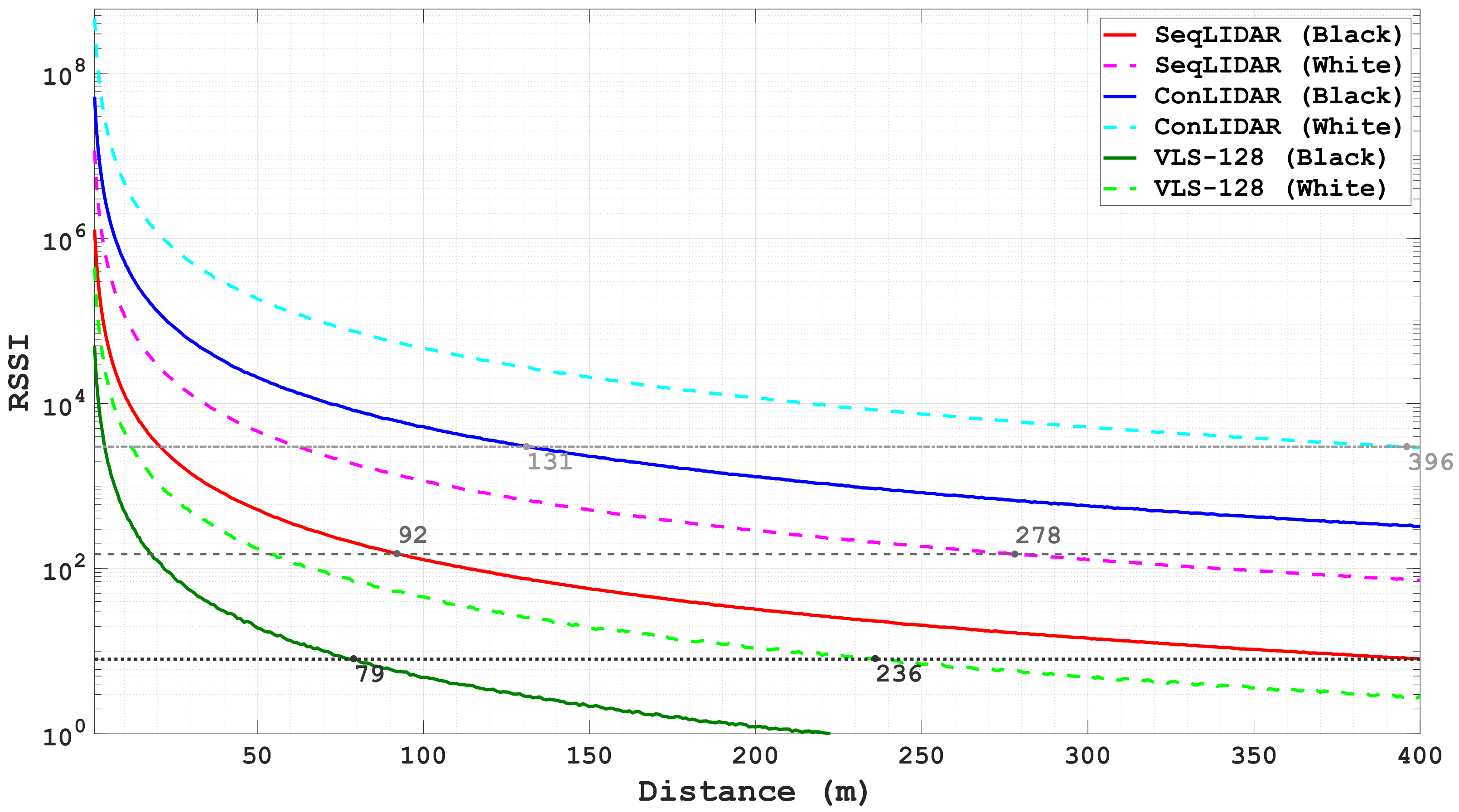
Figure 14 shows the maximum detectable distance using the received signal strength when measuring the white paper wall and black matte paper wall with the three LIDAR scanners. The sequential firing LIDAR scanner and the concurrent firing LIDAR scanner could detect signals that were not clearly distinguished from noise by using multiple reflected laser pulses. Compared to the black matte paper wall, the white paper wall had higher reflectivity, so all three LIDARs could equally measure a longer distance with the white paper wall. The laser output of the sequentially transmitted LIDAR scanner was lower than that of the VLS-128, but it was possible to detect reflected waves over a longer distance by using multiple reflected laser waves. The proposed concurrent firing LIDAR could transmit laser pulses with a power of several tens of times higher than that of sequential firing LIDAR or the VLS-128 by using laser pulses in the 1550 nm band instead of the 900 nm band and fewer pulses for multiplexing. As a result, the measurable distance was also longer than that of other LIDAR scanners.
After the pulse was reflected from the destination, the received signal strength was inversely proportional to the square of the distance to the destination. A strong signal was received when the distance to the destination was close, and a weak signal was received as the distance was increased. For this reason, when a large SNR was used, the received signal was clearly distinguished from noise, and the false alarm rate was very low; however, the measurement distance was shortened due to the need for a high received signal strength. If a low SNR were used, the false alarm rate would be high because the received signal is difficult to distinguish from noise, but the low received signal strength was required, so the range of maximum distance increased. In the case of LIDAR or radar, a large SNR is preferred because a low false alarm rate is important, and a high received signal strength is used. Each of the received signals was difficult to distinguish from noise, but when multiple pulses were used, it was possible to determine whether they had the same pattern as the transmitted signal by analyzing the pattern. Even if the power of a single pulse is distributed and transmitted, the transmission signal can be detected using a low SNR, so it is possible to measure a similar or distant place compared to the method using a single pulse.
Simulation results for the accuracy and precision of the positions are summarized in
Table 6 for better presentation. The accuracy and precision of the position were measured for the three LIDARs according to the standards of the American Society for Photogrammetry and Remote Sensing (ASPRS) [
40,
41]. Compared to the VLS-128, which uses one pulse, the sequential firing LIDAR scanner and concurrent firing LIDAR scanner had twice the accuracy and five to six times higher accuracy. Results suggested that the proposed concurrent firing LIDAR scanner that used multiple pulses performed much better than both sequential LIDAR scanners, as well as Velodyne’s state-of-the-art VLS-128 LIDAR.
5. Conclusions
This paper proposed a concurrent firing LIDAR scanner that compensates for the shortcomings of the sequential firing LIDAR scanner. The sequential firing LIDAR scanner implements multiplexing using an asynchronous prime sequence code and requires a large number of chips and the transmission of laser pulses to each target point. The proposed concurrent firing LIDAR scanner implements multiplexing by additionally using multiple wavelengths using a CHPC. By transmitting laser pulses of different wavelengths for every 128 elevation angle from one azimuth angle, one-hundred twenty-eight elevation angles can be measured at the same time. The concurrent firing LIDAR scanner can operate at a much higher speed than the sequential firing LIDAR scanner and Velodyne’s state-of-the-art VLS-128. The sequential firing LIDAR scanner and VLS-128 use the 900 nm band, which poses a serious threat to the human retina. In comparison, the proposed LIDAR scanner uses the 1550 nm band and has a slight influence on the human optic nerve.
Extensive simulations were performed to analyze the performance of the proposed LIDAR scanner, and results indicated that it was possible to use a laser power that was ten times higher than the traditional LIDAR scanners to measure even longer distances. Performance was analyzed for the 3D point cloud, measurable range and precision, and the accuracy of the measured distance. Results suggested that the proposed LIDAR performed better than both the sequential firing LIDAR scanner and state-of-the-art Velodyne VLS-128 LIDAR. The proposed LIDAR scanners use 384 laser diodes and photodiodes each in the 1550 nm band, which are expensive and become the biggest factor in the high price when commercialized. Depending on the target of the product, if a higher resolution is required, regardless of the price, a larger number of laser diodes and photodiodes can be used to increase the resolution as desired. On the other hand, if the product is price-critical, it is possible to reduce the number of laser diodes and photodiodes to match the desired product price.


