Abstract
The objective of this project is to create a new implementation of a deep learning model that uses digital elevation data to detect shipwrecks automatically and rapidly over a large geographic area. This work is intended to apply a new methodology to the field of underwater archaeology. Shipwrecks represent a major resource to understand maritime human activity over millennia, but underwater archaeology is expensive, misappropriated, and hazardous. An automated tool to rapidly detect and map shipwrecks can therefore be used to create more accurate maps of natural and archaeological features to aid management objectives, study patterns across the landscape, and find new features. Additionally, more comprehensive and accurate shipwreck maps can help to prioritize site selection and plan excavation. The model is based on open source topo-bathymetric data and shipwreck data for the United States available from NOAA. The model uses transfer learning to compensate for a relatively small sample size and addresses a recurring problem that associated work has had with false positives by training the model both on shipwrecks and background topography. Results of statistical analyses conducted—ANOVAs and box and whisker plots—indicate that there are substantial differences between the morphologic characteristics that define shipwrecks vs. background topography, supporting this approach to addressing false positives. The model uses a YOLOv3 architecture and produced an F1 score of 0.92 and a precision score of 0.90, indicating that the approach taken herein to address false positives was successful.
Keywords:
deep learning; machine learning; lidar; sonar; shipwrecks; archaeology; remotely sensed imagery 1. Introduction
1.1. Objective and Broader Importance
This project’s objective is to determine whether deep learning and open source high-resolution bathymetric data could be used to accurately predict the locations of shipwrecks over a large geographic area. This work is intended to introduce a new methodology to the field of underwater archaeology that can be used in conjunction with existing methodologies. Maritime shipwrecks represent a major resource to understand the human past over thousands of years, but underwater archaeology is expensive, misappropriated, and hazardous [1,2,3,4]. Therefore, a methodology to automatically map all potential shipwrecks over a large geographic area accurately and rapidly can help archaeologists prioritize site selection and plan excavation [5]. The model implementation presented here accurately detects shipwrecks in remotely sensed imagery collected from large areas of the coast of the continental United States, Alaska, and Puerto Rico. The methodological approach can easily be replicated in other locations around the world.
Machine learning applications in archaeology have made significant progress in predictive accuracy and utility in the last decade [6,7,8,9,10], with work over the last four years focused on the application of a specific type of machine learning algorithm called deep learning [11,12,13,14,15]. Deep learning is a type of machine learning that can identify features of interest in remotely sensed imagery by recognizing the unique visual patterns by which they are represented [16]. It is particularly powerful for detecting archaeological features because of its ability to identify many different morphologies and orientations of the same features. Applications of deep learning to underwater archaeology are very limited [12,17,18] because of the paucity of high-resolution bathymetric data [19] as compared to land-based elevation data. The new model implementation presented here uses high resolution open source bathymetric data accessed through the National Oceanic and Atmospheric Administration’s (NOAA) Office of Coastal Management Data Access Viewer [20], as well as the GPS locations of confirmed shipwrecks from NOAA’s Office of Coast Survey’s Automated Wreck and Obstruction Information System (AWOIS) database [21]. Part of NOAA’s mission is to document the seafloor to ensure natural resources are protected and waterways are navigable for mariners. This includes a database of more than 10,000 shipwrecks and underwater obstructions. This model will be used by the Navy’s Underwater Archaeology Branch to find unmapped or unknown naval shipwrecks to aid management objectives by creating more accurate and complete maps of shipwreck locations and by studying shipwreck patterns across the underwater landscape. This work seeks to make machine learning methods applicable and relevant to archaeologists and others interested in studying, managing, and conserving the maritime landscape.
1.2. Background and Related Literature
Machine learning here refers to the process of teaching a computer to seek and identify features that a human would otherwise have to locate and classify visually [22]. Deep learning is a type of machine learning that uses multiple layers of data to learn the patterns associated with the features of interest with little to no human guidance or associated bias. This enables deep learning models to essentially assess images in the same way that a human would: humans can look at pictures of a cat and a dog, for example, and immediately know which animal they are looking at because of physical features such as ear shape, snout shape, and coloration. Deep learning models create and then iterate through hundreds or thousands of layers of an image to automatically determine which combination of patterns are most likely to define the content of the image [16].
There are very few published studies that combine deep learning with remotely sensed imagery to detect shipwrecks over a large area, though there are several studies that use remotely sensed imagery to visually identify shipwrecks. Remotely sensed imagery can include imagery collected by satellite, airplane, unmanned aerial vehicle (UAV), ship, or autonomous underwater vehicle (AUV), and includes many types of elevation (e.g., lidar, sonar, synthetic aperture radar) and spectral (e.g., multispectral, hyperspectral) imagery sensors. The majority of published studies focused on shipwreck detection also rely on sonar imagery collected by AUV which restricts the size of the study area to what is immediately near the AUV, whereas the new work presented by the authors is based on a mosaic of airborne lidar and shipborne sonar collected over much larger areas (i.e., nearly the entire coast of the continental US, Alaska, and Puerto Rico). There is also a small corpus of work focused on using remotely sensed imagery to identify aircraft wrecks, which are sometimes located underwater. A brief chronologic review of related work follows that includes a variety of manual and machine learning methods applied to identifying submerged features in remotely sensed imagery.
In 2011 Plets et al. [23] assessed whether 2–4 m spatial resolution multibeam sonar could be used to manually detect possible wrecks on the seafloor. This appears to be the first study in the literature that attempts to use remotely sensed imagery to detect shipwrecks, and the authors note that this study was only possible because of the availability of relatively high-resolution imagery. In fact, this imagery is quite high resolution for the time. Nonetheless, the results of the study conclude that the spatial resolution of the imagery limited the identification of smaller, older vessels and that higher resolution—probably 1 m—is therefore required for a phase two of the project. This finding is aligned with the new work presented in this paper. In 2013 Shih et al. [24] used airborne bathymetric lidar data with a spatial resolution of 3.5 m to manually detect four shipwrecks around a coral reef located in the South China Sea. Similar to Plets et al. [23], the authors found that the spatial resolution of the lidar limited their ability to detect smaller wrecks. Nonetheless, Shih et al.’s study shows that airborne bathymetric lidar is effective in shipwreck identification. Since 2017, Pasquet et al. [12] and Drap et al. [5] have been working together on a project to develop a deep learning approach for the detection and recognition of objects of interest using orthomosaics, with a focus on amphorae. Using transfer learning to help address their small training dataset size (transfer learning is the process of using as a model base layer the output of another model that has been pretrained on many thousands of images of other features), they test their approach to detect amphorae at a single shipwreck site located in 44 m of water. They find that their model can detect about 90% of amphorae once noise is removed but does produce several false positives with a precision value ranging from 60 to 80%. This study highlights the more general utility of a deep learning approach to underwater feature detection and is at the forefront of other related projects.
Since 2018 there have been nearly as many publications as the previous decade. Most of these studies use side scan sonar and deep learning to detect wrecks. Ye et al. [25] created a deep learning model based on side scan sonar imagery that used transfer learning to detect shipwrecks and aircraft wrecks, reaching a classification accuracy rate of 87%. Nayak et al. [17] created a deep learning model to detect shipwrecks using side scan sonar and a small number of training sites combined with image augmentation (to increase the training dataset size). Their model was tested on two datasets: the model produced recall values between 80 and 97% and precision values between 29 and 33%. As is evidenced by the low precision values, the authors had problems with false positives similar to Pasquet et al. [12] and Drap et al. [5]. Xu et al. [26] used a neural network to detect shipwrecks in sonar imagery with a very small training dataset. They tested model performance both with and without transfer learning and found that transfer learning improved the model significantly: the model produced mean average precision values of 73% and 81% without transfer learning and with transfer learning, respectively. Zhu et al. [18] used a similar approach that included side scan sonar and transfer learning, but instead of deep learning they tested a variety of shallow learning approaches. The results of the various models ranged from correct recognition rates of 90–97%; the study does not include discussion of precision or false positives. The authors also suggest that model performance may be improved by implementing a deep learning approach. These studies all indicate that high resolution imagery and deep learning are successful approaches to identification of underwater wrecks. Additionally, they show that transfer learning is a successful way to address a small training dataset. All models presented in these studies have difficulty with false positives; an approach that can be used to address false positives is to include background topography examples in model training, something that none of these papers tested but that the new work presented here will include.
In a particularly relevant study published in 2020, Davis et al. [27] manually assessed the utility of NOAA’s open access 1 and 3 m resolution coastal bathymetric data for shipwreck identification. Manual identification was based on morphologic characteristics, including shape, elevation profile, and size of the anomaly. They focused on three study areas that had different water clarity and available imagery resolutions. They were able to manually detect 44% of wrecks in the Mississippi Delta study area off the coast of New Orleans. The area has an average water clarity of less than 1 m and the imagery they used had a spatial resolution of 3 m. The authors had more success in their other two study areas: they were able to detect 63% of wrecks in their study area off the coast of Long Island, New York and 61% in their study area off the coast of Massachusetts. Visibility in the Long Island Sound ranges from 0 to 3 m and there is 1m spatial resolution imagery available for this area. Visibility in the Boston Harbor usually averages 2.5 m. Imagery available for this study area includes both 1 and 3 m spatial resolution. The authors also tested the performance of an inverse detection analysis (IDA) algorithm with a 20 km2 section of the Long Island data to determine whether automated methods might have utility in wreck detection. IDA is a method of flipping the topographic surface inside-out such that sinks are represented as morphologically distinct anomalous mounds, or in this case as shipwrecks. Their model produces a true positive rate of 71% and a false negative rate of 28.67%, indicating that automated methods may have utility in shipwreck detection. In addition to lending support to the objective of the new work presented here to determine whether deep learning could be used to detect shipwrecks, Davis et al.’s work also helped the authors to rapidly identify training data for deep learning modeling.
2. Materials and Methods
2.1. Deep Learning Model
We completed all modeling in Python programming language and geospatial analyses in ArcGIS Pro. The deep learning model was run in Keras with a TensorFlow backend using a NVIDIA 1080 GEFORCE GTX GPU.
Training data consisted of GPS points of confirmed shipwrecks and associated bathymetric data. To create our training dataset of known shipwrecks, we explored bathymetric data for the entire US coastline, from Maine to Florida, from Florida to Louisiana, from California to Washington and to Alaska (excluding Hawaii), and all along the coast of Puerto Rico. Davis et al. [27] included maps and GPS coordinates for shipwrecks, which we used to rapidly identify areas that were likely to contain shipwrecks. The bathymetric data were acquired through NOAA’s Data Access Viewer [20] and the shipwreck GPS coordinates were acquired through NOAA’s AWOIS [21]. The bathymetric data used in modeling were derived from 1 m resolution lidar and multibeam sonar. The shipwreck training data used in the model consisted of 163 shipwrecks that were visible as some sort of anomalous morphology in the bathymetric data. These were augmented through stretching and orientation adjustments to produce an additional 247 varied shipwreck images. The total training dataset consisted of 410 shipwrecks. The training data also included 410 background topography tiles to help ensure that the model was able to differentiate between shipwrecks and topography. The test dataset consisted of 40 additional shipwrecks and 40 background topography tiles; no data augmentation was used in the test data.
We used ArcGIS Pro to derive hillshades from elevation data and then to export the hillshade tiles containing shipwrecks in png format, which were labeled using Microsoft’s Visual Object Tagging Tool [28].
The model architecture was based on Joseph Redmon’s convolutional neural network one-shot detector model YOLOv3 [29], and this specific implementation was developed based on two GitHub repositories: qqwweee’s keras-yolo3 [30] and AntonMu’s TrainYourOwnYOLO [31]. YOLOv3 was used for this work because of its high detection accuracy and very fast speed [29]. A basic explanation of the YOLOv3 framework follows. The YOLOv3 network framework can be divided into two components: a feature extractor and a detector (Figure 1). Each input image is automatically resized to a width and height of 416 × 416 pixels before entering the feature extractor. YOLOv3 uses Darknet53 which outputs feature maps at three different scales. These feature maps are then provided as input into the detector which initially predicts three bounding boxes. The most suitable bounding box out of the three is output by the detector, represented as the predicted bounding box center point, width and height, confidence, and class label. The model uses transfer learning, and weights were pretrained on the ImageNet1000 dataset [32].

Figure 1.
High-level schematic of YOLOv3.
For each test image, the output of the model was each input test image with bounding boxes drawn around predicted shipwrecks along with a confidence score representing how confident the model was in its prediction (Figure 2). These data are also output in a spreadsheet format.
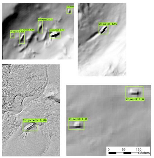
Figure 2.
Example of model output. Each of these is a sonar or lidar hillshade image that was provided to the model as input. The model outputs these same images with bounding boxes indicating the locations of predicted shipwrecks and an associated confidence score for the prediction.
We assessed model performance using a new set of test data and calculated several accuracy metrics, including area under curve receiver operating characteristic curve (AUC-ROC), precision–recall curve, overall accuracy, recall, precision, and F1 score [33,34].
A ROC curve shows the false positive rate on the x-axis compared to the true positive rate on the y-axis for different thresholds between 0 and 1 (Figure 3). Smaller values on the x-axis indicate a lower number of false positives and a higher number of true negatives. Larger values on the y-axis indicate higher true positives and lower false negatives. This metric enables model comparison either in general or for different thresholds. The AUC can also be used as a summary of the model’s predictive ability, or skill. A no-skill classifier cannot differentiate between the classes and is represented by a straight line that runs through the point (0.5, 0.5); the AUC of this curve is equal to 0. A model with perfect skill is represented by a line at a point (0,1); this line moves up from the bottom left of the plot to the top left of the plot and then moves horizontally across the plot to the top right. The AUC of this curve is equal to 1. Generally, an AUC-ROC score between 0.7 and 0.8 is acceptable, above 0.8 is excellent, and more than 0.9 is outstanding [35,36]. A precision–recall curve is a plot of the precision vs. the recall for different thresholds. A no-skill classifier, as with the AUC-ROC curve, is one that cannot differentiate between the classes. A model with perfect skill is represented by a point at (1,1) and a skillful model is represented by a curve above and bending toward the no-skill line. Since both AUC-ROC and precision–recall curves show model skill at many different thresholds, these metrics can be used to determine appropriate thresholds for the threshold-dependent metrics (accuracy, recall, precision, F1 score).
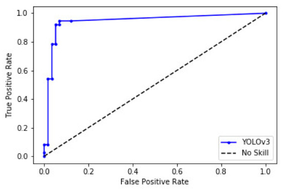
Figure 3.
AUC-ROC plot.
Overall accuracy is the number of overall correctly classified shipwrecks and background topography tiles as compared to the entire number of samples and is the only metric that considers true negatives (TN). Recall represents the prediction accuracy when considering only the true positives (TP) as compared to the total number of positives including false negatives (FN)—here this is equivalent to how many shipwrecks were correctly classified as shipwrecks. Precision minimizes the occurrence of false positives (FP), which in this case means that it decreases the model’s likelihood of mistaking background topography for a shipwreck. The flip side of this is that it may also cause the model to mislabel shipwrecks as background topography. Different accuracy metrics are more appropriate to use depending on the objective of the model.
2.2. Pattern and Statistical Analyses
We created box and whisker plots and histograms and ran one-way ANOVAs to look for patterns and significance in shipwreck locations and morphology. Parameters were calculated for areas immediately surrounding shipwrecks and were compared to background topography values used in model training. Parameters include slope, curvature (describes the overall shape of the slope), curvature-profile (parallel to direction of maximum slope), curvature-planar (perpendicular to direction of maximum slope), wreck area, wreck rectangularity, wreck distance from coast, wreck depth, nearest state to wreck, and water clarity above wreck.
Shipwreck values were compared to those of background topography for slope (degrees) and all curvatures. Shipwrecks values were not compared to background topography for all other parameters (wreck area, wreck rectangularity, wreck distance from coast, wreck depth, nearest state to wreck, and water clarity above wreck) because these parameters are wreck specific. For slope and all curvatures, minimum, mean, and maximum values were calculated; the maximum values consistently showed the most differentiation between the values for shipwrecks and the values for background topography. Empirically, this makes sense because the morphological parameters are capturing the man-made shape of the shipwrecks that includes more straight edges than are found in nature.
3. Results
3.1. Deep Learning Model
The AUC-ROC score of the final model for this project is 0.945 (Table 1; Figure 3). The AUC-Precision-Recall score of the final model for this project is 0.901 (Table 1; Figure 4). Additional accuracy metrics are shown in Table 1, as well.

Table 1.
Accuracy metric formulas and results for model.
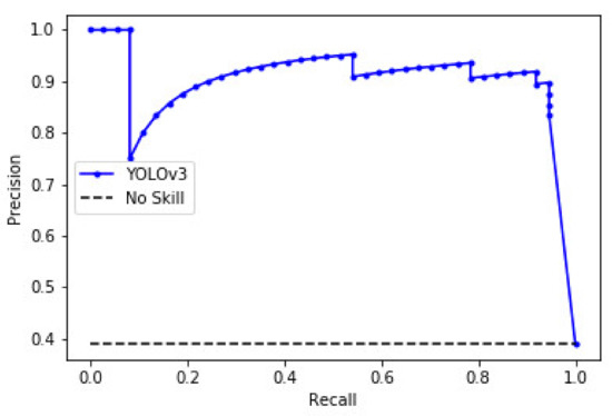
Figure 4.
AUC-Precision-Recall plot.
3.2. Pattern and Statistical Analyses
We found that shipwrecks have significantly higher slope values and curvature values (Figure 5) than those of background topography. The F ratios and p-values (Table 2) indicate that all parameters are significant, meaning that each of these parameters tend to share a distinct range of values for shipwrecks as compared to background topography.
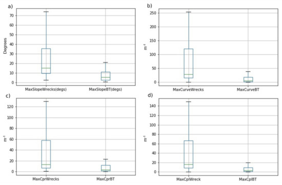
Figure 5.
Box and whisker plots comparing the (a) maximum slope, (b) curvature, (c) curvature-profile, and (d) curvature-planar of the shipwrecks to that of the background topography.

Table 2.
F ratios and p-values for all shipwreck vs. background topography parameters (alpha = 0.05).
On average, the total ground area occupied by an individual wreck was 1470 m2 (Figure 6). We hypothesized that on average wrecks would have a more rectangular than circular shape. To test this hypothesis, we created a rectangularity metric by subtracting the wreck area from the area of its minimum bounding rectangle and then normalizing the results so that everything fell between 0 and 1. Zero represents a perfect rectangle and the larger the number the less rectangular the shipwreck. The majority of wrecks used in this study were fairly rectangular in shape (Figure 7). We also hypothesized that the visibility of wrecks may correspond to a shipwreck’s state of preservation, with more decomposed wrecks appearing less rectangular. This hypothesis requires ground-verification, and many factors would contribute to preservation including age and environmental conditions such as anoxia and turbulence. The wrecks used in this study were all located in shallow water (<80 m), with low slope gradients, and relatively nearshore (<14 km; Figure 8). We also hypothesized that wreck visibility might be affected by water clarity. To empirically test this hypothesis, we created a water clarity scale and assessed water clarity at each shipwreck location using spectral satellite imagery provided as the ArcGIS base map (Figure 9). With over 90% of the wrecks occurring in opaque waters, this hypothesis does not seem to hold true (Table 3).
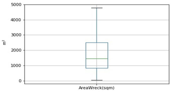
Figure 6.
Box and whisker plot showing wreck area in square meters (four extreme outliers have been removed to avoid skewing of data).
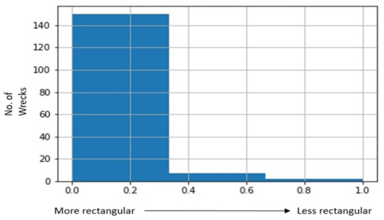
Figure 7.
Histogram showing wreck rectangularity where rectangularity is on the x-axis (0 is perfect rectangle, larger numbers are less rectangular) and count is on the y-axis (four extreme outliers have been removed to avoid skewing of data).
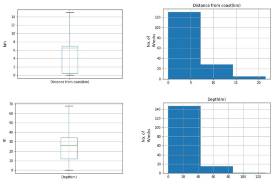
Figure 8.
Box and whisker plot and histograms showing wreck distance from coast in kilometers and wreck depth in meters.
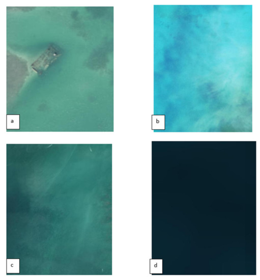
Figure 9.
Examples of water clarity. (a) is above water, (b) is transparent, (c) is translucent, (d) is opaque.

Table 3.
Observed water clarity at each wreck site.
4. Discussion
NOAA’s bathymetric data includes a range of spatial resolutions, but we found that a 1 m resolution was ideal for detecting shipwrecks. Wrecks were occasionally detectable in 3 m resolution imagery, so this imagery could potentially be used in future modeling. This finding is aligned with manual shipwreck identification conducted by Plets et al. [26], from which the authors conclude that the required imagery resolution for shipwreck identification is less than 2 m. Fewer than 10 shipwrecks that we detected were easily discernible (Figure 10), while most wrecks appeared simply as anomalous topography (Figure 11). In addition to the spatial resolution of bathymetric data, wreck detection was affected by water depth and clarity. The largest number of wrecks detected were in the Long Island Sound (90 wrecks: Table 4) and the Puget Sound (50 wrecks: Table 4). A smaller number of wrecks were also detected in Boston Harbor, Delaware Bay, in the Florida Keys, and off the coast of Puerto Rico (Table 4). Wrecks were not detected in the sediment-laden Gulf of Mexico. The detectability and general profusion, or lack thereof, of wrecks is likely tied to such factors as water clarity and depth, imagery spatial resolution, and wreck preservation, as well as historic, commercial, and naval factors not discussed in this paper. The performance of new model implementations therefore is likely to vary based on the differing influence of these factors across geographic locations.
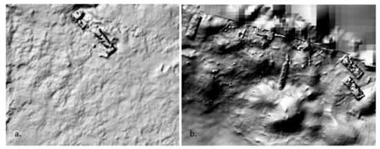
Figure 10.
Obvious shipwrecks off the coast of Puerto Rico (a) and Washington (b) at a depth of 3 and 25 m, respectively.
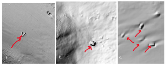
Figure 11.
Less obvious shipwrecks with arrows above were more common than the type shown in Figure 9. These shipwrecks in (a,b) occur off the coast of Washington and in (c) off the coast of Connecticut/New York, at a water depth of 29 (a), 60 (b), and 45 (c) m, respectively.

Table 4.
Table of the nearest state to where the model identified shipwrecks. The Long Island Sound off the coast of Connecticut and the Puget Sound off the coast of Washington had by far the largest number of highly visible wrecks, containing 59% and 31% of wrecks, respectively.
The work presented in Davis et al. [30] is the most similar study to date to the project presented here. Davis et al. used IDA to identify wrecks in a small section of the Long Island Sound, achieving a recall of 71%. The YOLOv3 model implementation used for this study achieved a recall of 95%. However, these two models did not use identical datasets, therefore a direct comparison is not possible.
All other published related work focuses either on a very small study area that includes fewer than four shipwrecks [5,12,24] or used privately available side scan sonar [17,18,25,26]. While some of these projects produce shipwreck detection results comparable with the new work presented here, the work presented here differs in three significant ways: (1) the study area is very large, which enables rapid mapping of huge areas all at once; (2) the imagery is open source, which means this methodology could be replicated for additional study areas; (3) the imagery used includes a substantial amount of airborne lidar which means that imagery can be efficiently collected over a much larger area than with a shipborne or unmanned platform. Additionally, excluding Nayak et al. [17], the projects that use side scan sonar are not focused on developing methodologies for underwater archaeology. Nayak et al. use side scan sonar collected by AUV, which limits the geographic extent of the project. Additionally, their model produces many false positives, as do the models introduced by Pasquet et al. [12] and Drap et al. [5]. The new model implementation presented here addresses false positives by integrating background topography in model training, achieving the highest precision value (90%) among these works by a large margin. Precision values of other works range from 29–33% [17] to 60–80% [5,12].
This work demonstrates the utility of deep learning methods to detect shipwrecks in high resolution bathymetric imagery, thus providing a new methodologic approach for underwater archaeology projects. Future work to further improve model performance and generalizability includes gathering a larger and more diverse training dataset. This could include integrating a larger number of less readily discernable wrecks from NOAA’s wreck database, searching for other in-country sources of data, and looking for some international data sources. Different approaches to digital elevation data visualization may also improve model performance. For this project we used hillshade, but we would also like to test model performance using other visualizations such as Local Relief Model (LRM), Red Relief Image Map (RRIM), and topographic openness. Lastly, we plan to test several different types of deep learning model architectures including a two-shot detector (two-shot detectors are significantly slower and more computationally intensive than one-shot detectors like YOLOv3, but they also can be more accurate) such as the Faster R-CNN [37], as well as shallow learning models based on shipwreck morphology, such as a random forest or gradient boosting. Given that there are strong morphological patterns that characterize both the shipwrecks and their locations on the seafloor, shallow learning could also offer a successful approach to predictive modeling. Future work as part of running this model implementation on a larger dataset that may produce many more false negatives also includes determining morphologic thresholds for slope and curvature, and potentially other parameters, that may define whether the model is able to detect a shipwreck. Future work could also use this rich database and approach to improve our knowledge of the causes and trends of historical shipwrecks such as tropical cyclones [38].
5. Conclusions
This paper presents a new highly accurate archaeological implementation of a deep learning model that uses digital elevation data derived from airborne lidar and shipborne sonar to automatically detect shipwrecks over a large geographic area. The model achieved a F1 score of 0.92, which means that the model is effectively able to detect shipwrecks in the test dataset used for this work. Additionally, the model achieved a precision value of 0.90, demonstrating that the incorporation of background topography into model training helps to resolve issues that previous models have had with false positives. Furthermore, statistical analyses show that there are substantial differences between the morphologic values for shipwrecks as compared to background topography, supporting our background topography-inclusive approach. This open source data-based approach facilitates research in underwater archaeology, providing a new methodology that can be used in conjunction with existing methodologies.
This model could enable marine archaeologists to quickly and efficiently detect potential unknown or unmapped shipwrecks, promoting conservation and management objectives. The model is now ready to ingest new, never-before-seen data and predict potential unmapped or unknown shipwreck locations. This could save the Navy’s Underwater Archaeology Branch person-hours or even days of visually searching data for features. Additionally, the methodology developed for this project could easily be modified to accept other types of images, such as multispectral imagery. It could also be altered to focus on other types of features, such as aircraft wrecks, naval mines, land-based archaeological features, or even geological features.
This work helps to bridge the gap between the field of machine learning pursued by computer scientists and the types of applied projects of interest to archaeologists, environmental scientists and others who seek to improve management and conservation practices. This project helps to make the cutting-edge research being done by computer scientists applicable and relevant to land and resource conservation and management work.
Author Contributions
Conceptualization, L.C. and A.O.J.; methodology, L.C.; software, L.C.; formal analysis, L.C.; investigation, L.C.; visualization, L.C.; writing—original draft preparation, L.C.; writing—review, writing, and editing, L.C., A.O.J., T.B., and S.L.-B.; funding acquisition, L.C. All authors have read and agreed to the published version of the manuscript.
Funding
This research was funded by the 2020 Naval Research Enterprise Internship Program (NREIP).
Data Availability Statement
Data available on request due to ethical restrictions. The data presented in this study are available on request from the corresponding author. The data are not publicly available due to ethics of archaeological site protection.
Acknowledgments
The authors thank all the anonymous reviewers and journal editorial staff for their help improving the quality of this manuscript. The first author would like to thank the Karl W. Butzer Excellence Fund for supporting her broader work to create methodologies for archaeologic machine learning.
Conflicts of Interest
The authors declare no conflict of interest.
References
- Bowens, A. Underwater Archaeology: The NAS Guide to Principles and Practice, 2nd ed.; Blackwell Publishing: Chichester, UK, 2011. [Google Scholar]
- Goggin, J. Underwater archaeology: Its nature and limitations. Am. Antiq. 1960, 25, 348–354. [Google Scholar] [CrossRef]
- McCarthy, J.K.; Benjamin, J.; Winton, T.; van Duivenvoorde, W. 3D Recoding and Interpretation for Marine Archaeology; Springer: Cham, Switzerland, 2019. [Google Scholar] [CrossRef]
- Wickham-Jones, C. Studying Scientific Archaeology: Landscape Beneath the Waves: The Archaeological Investigation of Underwater Landscapes; Oxbow: Oxford, UK, 2019; Volume 4. [Google Scholar]
- Drap, P.; Papini, O.; Merad, D.; Pasquet, J.; Royer, J.-P.; Nawaf, M.M.; Saccone, M.; Ben Ellefi, M.; Chemisky, B.; Seinturier, J.; et al. Deepwater archaeological survey: An interdisciplinary and complex process. In 3D Recording and Interpretation for Maritime Archaeology; McCarthy, J.K., Benjamin, J., Winton, T., van Duivenvoorde, W., Eds.; Springer: Cham, Switzerland, 2019; pp. 135–153. [Google Scholar] [CrossRef]
- Davis, D.S. Object-based image analysis: A review of developments and future directions of automated feature detection in archaeology. Archaeol. Prospect. 2018, 26, 155–163. [Google Scholar] [CrossRef]
- Davis, D.S. Defining what we study: The contribution of machine automation in archaeological research. Digit. Appl. Archaeol. Cult. Herit. 2020, 18, e00152. [Google Scholar] [CrossRef]
- Luo, L.; Wang, X.; Guo, H.; Lasaponara, R.; Zong, X.; Masini, N.; Wang, G.; Shi, P.; Khatteli, H.; Chen, F.; et al. Airborne and spaceborne remote sensing for archaeological and cultural heritage applications: A review of the century (1907–2017). Remote Sens. Environ. 2019, 232, 111280. [Google Scholar] [CrossRef]
- Rosenzweig, M.S. Confronting the Present: Archaeology in 2019. Am. Anthropol. 2020, 122, 284–305. [Google Scholar] [CrossRef]
- Sevara, C.; Pregesbauer, M.; Doneus, M.; Verhoeven, G.; Trinks, I. Pixel versus object–A comparison of strategies for the semi-automated mapping of archaeological features using airborne laser scanning data. J. Archaeol. Sci. Rep. 2016, 5, 485–498. [Google Scholar] [CrossRef]
- Caspari, G.; Crespo, P. Convolutional neural networks for archaeological site detection–Finding “princely” tombs. J. Archaeol. Sci. 2019, 110, 104998. [Google Scholar] [CrossRef]
- Pasquet, J.; Demesticha, S.; Skarlatos, D.; Merad, D.; Drap, P. Amphora detection based on a gradient weighted error in a convolutional neural network. In Proceedings of the IMEKO International Conference on Metrology for Archaeology and Cultural Heritage, Lecce, Italy, 23–25 October 2017. [Google Scholar]
- Somrak, M.; Dzeroski, S.; Kokalj, Z. Learning to classify structures in ALS-derived visualizations of ancient Maya settlements with CNN. Remote Sens. 2020, 12, 2215. [Google Scholar] [CrossRef]
- Trier, O.D.; Cowley, D.C.; Waldeland, A.U. Using deep neural networks on airborne laser scanning data: Results from a case study of semi-automatic mapping of archaeological topography on Arran, Scotland. Archaeol. Prospect. 2019, 26, 165–175. [Google Scholar] [CrossRef]
- Van der Vaart, V.; Wouter, B.; Lambers, K. Learning to Look at LiDAR: The Use of R-CNN in the Automated Detection of Archaeological Objects in LiDAR Data from the Netherlands. J. Comput. Appl. Archaeol. 2019, 2, 31–40. [Google Scholar] [CrossRef]
- Chollet, F. Deep Learning with Python; Manning Publications Co.: New York, NY, USA, 2018. [Google Scholar]
- Nayak, N.; Nara, M.; Gambin, T.; Wood, Z.; Clark, C.M. Machine learning techniques for AUV side scan sonar data feature extraction as applied to intelligent search for underwater archaeology sites. Field Serv. Robot. 2021, 16, 219–233. [Google Scholar] [CrossRef]
- Zhu, B.; Wang, X.; Chu, Z.; Yang, Y.; Shi, J. Active learning for recognition of shipwreck target in side-scan sonar image. Remote Sens. 2019, 11, 243. [Google Scholar] [CrossRef]
- Wölff, A.-C.; Snaith, H.; Amirebrahimi, S.; Devey, C.W.; Dorschel, B.; Ferrini, V.; Huvenne, V.A.I.; Jakobsson, M.; Jencks, J.; Johnstone, G.; et al. Seafloor mapping—The challenge of a truly global bathymetry. Front. Mar. Sci. 2019, 6, 283. [Google Scholar] [CrossRef]
- NOAA Dataviewer. Available online: https://coast.noaa.gov/dataviewer/#/lidar/search/ (accessed on 30 March 2021).
- NOAA Wrecks and Obstructions Database. Available online: https://nauticalcharts.noaa.gov/data/wrecks-and-obstructions.html (accessed on 30 March 2021).
- Géron, A. Hands-On Machine Learning with Scikit-Learn, Keras, and TensorFlow: Concepts, Tools, and Techniques to Build Intelligent Systems; O’Reilly Media, Inc.: Newton, MA, USA, 2019. [Google Scholar]
- Plets, R.; Quinn, R.; Forsythe, W.; Westley, K. Using multibeam echo-sounder data to identify shipwreck sites: Archaeological assessment of the Joint Irish Bathymetric Survey data. Int. J. Naut. Archaeol. 2011, 40, 87–98. [Google Scholar] [CrossRef]
- Shih, P.T.-Y.; Chen, Y.-H.; Chen, J.C. Historic shipwreck study in Dongsha Atoll with bathymetric LiDAR. Archaeol. Prospect. 2013, 21. [Google Scholar] [CrossRef]
- Ye, X.; Li, C.; Zhang, S.; Yang, P.; Li, X. Research on side-scan sonar image target classification method based on transfer learning. In Proceedings of the OCEANS MTS/IEEE, Charleston, SC, USA, 22–25 October 2018. [Google Scholar]
- Xu, L.; Wang, X.; Wang, X. Shipwrecks detection based on deep generation network and transfer learning with small amount of sonar images. In Proceedings of the IEEE 8th Data Driven Control and Learning Systems Conference, Dali, China, 24–27 May 2019. [Google Scholar]
- Davis, D.S.; Buffa, D.C.; Wrobleski, A.C. Assessing the utility of open-access bathymetric data for shipwreck detection in the United States. Heritage 2020, 3, 22. [Google Scholar] [CrossRef]
- GitHub. Repository for Microsoft’s Visual Object Tagging Tool. Available online: https://github.com/microsoft/VoTT (accessed on 30 March 2021).
- Redmon, J.; Farhadi, A. YOLOv3: An Incremental Improvement. arXiv 2018, arXiv:1804.02767v1. [Google Scholar]
- GitHub. Repository for YOLOv3, Qqwweee. Available online: https://github.com/qqwweee/keras-yolo3 (accessed on 30 March 2021).
- GitHub. Repository for YOLOv3, Anton Mu. Available online: https://github.com/AntonMu/TrainYourOwnYOLO (accessed on 30 March 2021).
- ImageNet1000. 2015. Available online: http://image-net.org/challenges/LSVRC/2015/index (accessed on 30 March 2021).
- Brownlee, J. How to use ROC Curves and Precision-Recall Curves for Classification in Python. Available online: https://machinelearningmastery.com/roc-curves-and-precision-recall-curves-for-classification-in-python/ (accessed on 30 March 2021).
- Accuracy Trap! Pay Attention to Recall, Precision, F-score, AUC. Available online: https://medium.com/datadriveninvestor/accuracy-trap-pay-attention-to-recall-precision-f-score-auc-d02f28d3299c (accessed on 30 March 2021).
- Hosmer, D.W., Jr.; Lemeshow, S.; Sturdivant, R.X. Applied Logistic Regression; John Wiley and Sons: Hoboken, NJ, USA, 2013. [Google Scholar]
- Mandrekar, J.N. Receiver operating characteristic curve in diagnostic test assessment. J. Thorac. Oncol. 2010, 5, 1315–1316. [Google Scholar] [CrossRef] [PubMed]
- Ren, S.; He, K.; Girshick, R.; Sun, J. Faster R-CNN: Toward Real-Time Object Detection with Region Proposal Networks. arXiv 2015, arXiv:1506.01497. [Google Scholar] [CrossRef] [PubMed]
- Trouet, V.; Harley, G.L.; Domínguez-Delmás, M. Shipwreck Rates Reveal Caribbean Tropical Cyclone Response to Past Radiative Forcing. Proc. Natl. Acad. Sci. USA 2016, 113, 3169–3174. [Google Scholar] [CrossRef] [PubMed]
Publisher’s Note: MDPI stays neutral with regard to jurisdictional claims in published maps and institutional affiliations. |
© 2021 by the authors. Licensee MDPI, Basel, Switzerland. This article is an open access article distributed under the terms and conditions of the Creative Commons Attribution (CC BY) license (https://creativecommons.org/licenses/by/4.0/).