Article

A Submonthly Surface Water Classification Framework via Gap-Fill Imputation and Random Forest Classifiers of Landsat Imagery

1
Department of Statistics, Iowa State University, Ames, IA 50011, USA
2
Department of Geological and Atmospheric Sciences, Iowa State University, Ames, IA 50011, USA
*
Author to whom correspondence should be addressed.
Remote Sens. 2021, 13(9), 1742; https://doi.org/10.3390/rs13091742
Submission received: 22 March 2021 / Revised: 20 April 2021 / Accepted: 26 April 2021 / Published: 30 April 2021
(This article belongs to the Section Remote Sensing in Geology, Geomorphology and Hydrology)

Abstract

:
Global surface water classification layers, such as the European Joint Research Centre’s (JRC) Monthly Water History dataset, provide a starting point for accurate and large scale analyses of trends in waterbody extents. On the local scale, there is an opportunity to increase the accuracy and temporal frequency of these surface water maps by using locally trained classifiers and gap-filling missing values via imputation in all available satellite images. We developed the Surface Water IMputation (SWIM) classification framework using R and the Google Earth Engine computing platform to improve water classification compared to the JRC study. The novel contributions of the SWIM classification framework include (1) a cluster-based algorithm to improve classification sensitivity to a variety of surface water conditions and produce approximately unbiased estimation of surface water area, (2) a method to gap-fill every available Landsat image for a region of interest to generate submonthly classifications at the highest possible temporal frequency, (3) an outlier detection method for identifying images that contain classification errors due to failures in cloud masking. Validation and several case studies demonstrate the SWIM classification framework outperforms the JRC dataset in spatiotemporal analyses of small waterbody dynamics with previously unattainable sensitivity and temporal frequency. Most importantly, this study shows that reliable surface water classifications can be obtained for all pixels in every available Landsat image, even those containing cloud cover, after performing gap-fill imputation. By using this technique, the SWIM framework supports monitoring water extent on a submonthly basis, which is especially applicable to assessing the impact of short-term flood and drought events. Additionally, our results contribute to addressing the challenges of training machine learning classifiers with biased ground truth data and identifying images that contain regions of anomalous classification errors.

1. Introduction

Remote sensors gather observations of Earth’s surface and atmosphere in a wide range of spectral, temporal, and spatial resolutions [1]. Data collected by these sensors are often classified at the pixel level to produce land cover maps of the Earth’s surface [2,3,4]. However, the accuracy and scope of analysis of these maps are significantly affected by factors such as spatial and temporal resolution, presence of cloud cover, and cost of acquisition of the remote sensing imagery [5]. Trade-offs that compromise the fidelity of one factor for the sake of another are often inevitable. Yet, recent advances in computation and open access to Landsat sensor data have led to the generation of high-resolution global land cover maps such as the European Joint Research Centre’s (JRC) Monthly Water History v1.0 dataset, which provides 30-m resolution global classifications of surface water at monthly intervals from 1984 to 2015 [4,6].
Open access to Landsat imagery has greatly advanced research in land cover classification studies [5,7]. The mapping of surface water and inland waterbodies using Landsat imagery has been of primary interest in a variety of studies [8,9,10,11]. Landsat images have a spatial resolution of 30 m and a temporal resolution of 8 or 16 days [6]. The Landsat 5, 7, and 8 satellites have generated a dataset of global imagery spanning from the early 1980s to the present day. Each satellite quantifies spectral information from surface reflectance in both the visible and infrared spectra. However, compared to aerial imagery, lower resolution and the presence of cloud cover pose challenges for consistent and accurate land cover classification from Landsat imagery. The Landsat 7 satellite is additionally affected by scan line corrector (SLC) failure which introduces additional gaps in its images [12].
Despite these challenges, many studies have mapped surface water using Landsat imagery [4,5,7,13,14]. The JRC Monthly Water History v1.0 dataset provides high resolution classification maps of surface water at monthly intervals to track the change in surface water extent over time and monitor the occurrence of floods and droughts [4]. This dataset classifies each pixel as open water, non-water, or missing at monthly intervals from 1984-2015. According to the JRC definition, areas classified as open water must contain 30 m 2 of water alone. The study claims a false positive water classification rate of less than 1 % and an exclusion rate of less than 5 % of true open water pixels.
While the success of the JRC Monthly Water History dataset is impressive, the data is most adept for studies of large waterbodies and regions of interest. Our initial studies of small waterbodies in Iowa using the JRC dataset, revealed that the stringent JRC definition (classifying as water only pixels composed of completely open water) often leads to underestimation of the total extent of small waterbodies and flooded wetlands. There are, in fact, a variety of signals that may characterize surface water, including pixels capturing (1) completely open water, (2) water along waterbody boundaries, or (3) water in wetland areas [7]. Additionally, the JRC dataset combines all Landsat imagery from each month into monthly classifications. This strategy does not always produce a gap-free classification map [4,11]. Furthermore, the monthly period between JRC classifications fails to capture the change of extent in waterbodies that occurs within each month, particularly in waterbodies with high seasonal fluctuation or those prone to short-term flooding and drought. By gap-filling every available Landsat image, the full temporal frequency of Landsat imagery can be retained to produce submonthly surface water classification maps.
There is a need for a classification framework that can classify a variety of surface water land covers with high sensitivity and retain the full temporal frequency of Landsat observations through gap-fill imputation. We developed the Surface Water IMputation (SWIM) classification framework using R and the Google Earth Engine computing platform to support analyses of small waterbodies with optimized sensitivity and temporal frequency. Our work has achieved several novel and important contributions. Most importantly, the SWIM classification framework includes gap-fill imputation to allow for classification of every pixel in each available Landsat image, even those where some or all of the region of interest is covered by clouds. Our case studies demonstrate that SWIM water extent estimations in images with a high proportion of imputed data are reliable and consistent with overall trends. Additionally, we show that it is possible to improve the accuracy of machine learning classifiers trained on error-prone and/or biased ground truth data via a novel cluster-based bias correction algorithm. Finally, we have developed a method to recognize anomalous classification results via outlier detection. We expect other scientists may be interested in applying SWIM to surface water analyses in studies that require submonthly classification frequency. For instance, we demonstrate in several case studies that the SWIM classification framework can more accurately identify the impact of short-term flood and drought events given its submonthly classification frequency compared to the JRC Monthly Water History dataset.
This paper is organized in the following sections. Section 2 describes the methodology of the SWIM classification framework. Our validation study is presented in Section 3.1, where we compare the SWIM classifications to the JRC classifications. In Section 3.2, three case studies demonstrate the advantages of studying waterbody dynamics with submonthly classification frequency using SWIM. The final sections of the paper, discuss and draw conclusions about the contributions of our research and its potential future directions.

2. Materials and Methods

The SWIM classification framework integrates a series of methods using R and the Google Earth Engine (GEE) computing platform to produce submonthly surface water classifications. In this section of the paper, we describe these methods and contextualize the contributions of each.
GEE allows researchers to rapidly process massive remote sensing datasets via both traditional and machine learning techniques [15]. The platform drastically reduces the complexity of acquiring and pre-processing such imagery. We utilize GEE for the first two steps of the SWIM classification framework, including gathering all Landsat imagery for the ROI and preparing the training data. GEE also includes a variety of out-of-the-box methods for supervised and unsupervised pixel classification. The training data and all other Landsat images for the ROI may be either classified on GEE directly or downloaded for further processing before classification. The gap-fill imputation and outlier detection steps of SWIM require downloading the data from GEE and performing these last steps in R. For generality, adjustable parameters of the SWIM classification framework are presented and our selected values are also specified, e.g., k = 3 .
The steps of the SWIM classification framework include gathering the Landsat imagery (Section 2.1), preparing the training data (Section 2.2), performing a clustering algorithm on the training data to improve classification sensitivity (Section 2.3), gap-filling missing values in the images (Section 2.4), classifying the images via random forest (Section 2.5), and identifying classification outliers (Section 2.6). These steps are visually summarized in Figure 1.

2.1. Gather Landsat Imagery

The coordinates of the ROI are stored in GEE as a polygon. GEE can efficiently compile all Landsat images that fall within this ROI and pre-process the data for classification.
  • Collect image population: Use GEE to collect all Landsat 5, 7, and 8 Surface Reflectance Tier 1 images with at least one pixel located within the ROI and clip each image to the ROI polygon. In regions with snow or frozen water during the winter months, we exclude images under these conditions.
  • Import JRC data: Merge each of the retained images with the JRC water classification layer of the same month and year as each image’s acquisition date.
  • Nullify low quality pixels: Utilize the Landsat quality assurance bands to nullify pixels containing cloud cover or other sensor errors as described in Appendix A [16].
  • Perform feature selection: The spectral channels provided in each of the images may be used directly for classification or functions of these bands may be used to generate other features. The six standard reflectance bands among Landsat mission imagery include Red, Green, Blue, NIR (Near Infrared), SWIR_1 (Shortwave Infrared 1), and SWIR_2 (Shortwave Infrared 2) [6]. Various forms of the Normalized Difference Water Index (NDWI, MNDWI) and other indices related to the infrared Landsat sensor bands have consistently been shown to perform well as features for detecting surface water [10,17,18,19]. We utilize the following quantities as features:
    (a)
    NDWI = ( Green NIR ) / ( Green + NIR ) [20,21]
    (b)
    MNDWI = ( Green SWIR_1 ) / ( Green + SWIR_1 ) [22]
    (c)
    SWIR_1 [23]

2.2. Select Training Images

From the full set of Landsat images compiled for the ROI, several high quality images are sampled as training data. Computational limits in GEE constrain the amount of training data that can be used for the within-platform random forest classifier, so we sample k = 3 training images for each ROI.
  • Filter low quality images: Filter the collected images, requiring each retained image to meet the following thresholds: no more than c % of the ROI is covered by clouds and at least a % of the ROI is included in the image (Appendix A). Values of c = 5 and a = 95 allow for a sufficient pool of high-quality imagery for the validation study presented in Section 3.1. We select images only from the Landsat 5 archive for training, but Landsat 7 and 8 images can also be used.
  • Sort imagery: Calculate the day of year (DOY) quantities from each image acquisition date and sort the images into k sets { D 1 , , D k } . In this implementation, we use DOY 120–180, DOY 180–240, and DOY 240–300 to split the growing season into three groups.
  • Select representative training imagery: For the images in each group, calculate the total number of pixels labeled as water in the JRC classification layer and sort the images by total JRC water extent in increasing order. Determine which image is the first to fall within the p th percentile for the group and select this image to represent the associated DOY range. We select p = 90 for our analyses. At this level, some of the selected images exhibit signal variation due to frequent flooding, which helps the classifier account for a range of surface water conditions.
The k images selected in this step can be used as training data for the random forest classifier within GEE or downloaded for use with other platforms such as R.

2.3. Cluster-Based Bias Correction Algorithm

In our initial studies, we used the sampled images and the associated JRC classification labels to train random forest classifiers for multiple ROI. The sensitivity of the classifier was low, with many majority water pixels classified as not water. As a solution to adjust for the bias in the ground truth JRC labels, we developed the Cluster-based Bias Correction (CBC) algorithm.
  • Cluster image: Given an image containing a set of pixels with b bands and the associated “ground truth” labels, use X-Means clustering [24] to assign each pixel to one of X clusters, such that X { x a , , x b } . For this study, we used x a = 10 and x b = 100 in order to ensure at least 10 clusters would be identified in the training images. This specification often results in regions of each waterbody being separated into various clusters based on different depths, bordering terrains, or vegetation. X-means clustering intrinsically determines the optimal number of clusters X by minimizing AIC. Perform clustering on the b bands for each pixel alone, without including the information from the ground truth labels.
  • Calculate proportion water: For each cluster x { 1 , , X } , calculate the proportion p [ 0 , 1 ] of pixels with an associated binary label of 1 or with at least one vertically or horizontally adjacent pixel labeled as 1. These adjacent pixels assist in identifying pixels located along the border of waterbodies.
  • Threshold at λ : For cluster x, if the proportion p is greater than a threshold λ [ 0 , 1 ] , i.e., p > λ , set a temporary classification label to 1 for all pixels belonging to cluster x. If p λ , set the temporary label to 0 for all pixels belonging to cluster x.
  • Compare to JRC label: After iterating through all X clusters, compare the temporary label for each pixel to its original label. If the temporary and original labels are both 1 or both 0, include one copy of the pixel data with the original label in the new training dataset. If the temporary and original labels do not match, include two copies of the pixel data in the training dataset, the first labeled 0 and the second labeled 1.
  • Sensitivity analysis: The threshold λ is selected in the validation study to reach desirable rates of sensitivity and specificity. See details in Section 3.1.
The goal of this technique is to generate a variation of the training label data that decreases local classification errors by reducing the effect of biases in the “ground truth” training labels. In the case that the CBC algorithm generates two copies of a pixel, one with label 0 and the other with label 1, we hypothesize the trained classifier is better able to accommodate for the uncertainty of the true label for these pixels. As a result, there is better quantification of the average nature of similar pixels for both classes.
The CBC algorithm is relatively simple as it was initially created within the constraints of GEE. The technique was also developed to work specifically with the bagging procedure of the random forest algorithm and may not perform similarly with other classification methods [25]. This algorithm is an integral part of the SWIM classification framework and outputs vary based on the value of λ . Section 3.1 includes a validation study that compares the classification results under various values of λ to the original JRC classifications.

2.4. Impute Missing Values

Remote sensing imagery collected via satellites is often contaminated by cloud cover or other sensor errors. Many classification techniques, such as those used to generate the JRC dataset, combine multiple images to fill in missing pixels. Gap-fill techniques can also be used to fill in gaps in Landsat imagery [26,27,28,29]. In order to avoid a reduction in temporal frequency, SWIM gap-fills missing pixels in each image using the spatio-temporal imputation algorithm STFIT [30]. By imputing each image, classifications can be generated for every pixel in all available imagery retaining the full temporal frequency of Landsat observations. This differentiates our method from another [31], which also used gap-filling to estimate surface water extent from Landsat imagery, but has a monthly temporal frequency at best.
Imputation is not performed on the training data to prevent the introduction of any potential bias into the classifier. For all other available imagery of the ROI, a modified version of the STFIT algorithm is used to fill in any gaps in each image before classification [30]. In the first step of the SWIM classification framework, we use GEE to gather all Landsat imagery of the ROI. Quality assurance bands are used to nullify pixels containing cloud cover for imputation as described in Appendix A [16]. The following procedures are used to impute missing values in these images:
  • Mean estimation: Group images by every two consecutive years (the last group containing three years if the total number of years is odd), then estimate a pixel-wise annual mean function within each group separately. Compared to using all of the images to estimate one universal mean function in STFIT, the proposed step mean estimation can reflect long-term waterbody extent variation and is more accurate when the annual mean of any pixel is nonstationary.
  • Temporal effect estimation: Subtract the estimated mean function from the observed pixels (i.e., calculate the residuals within each group after removing outliers), then pass the residuals to the temporal effect estimation in the STFIT algorithm.
  • Spatial effect estimation: The STFIT algorithm is used to estimate the spatial effect for pixels in partially missing images by sparse FPCA techniques [32]. For images with completely missing data, we use a linear interpolation of the spatial effect estimates from the nearest before and after images by date (of those with less than 50 % pixels missing) to estimate the spatial effect.
  • Imputation: The imputed pixel value is the sum of the mean estimate, temporal effect estimate, and spatial effect estimate.
This step of the SWIM classification framework must be performed in R after downloading the Landsat data for the ROI. The procedure is efficient for imputing images of a few thousand pixels. For the case study ROIs in Section 3.2, we implemented a 2-level hierarchical sampling scheme to reduce the computational burden [30]. A sub-image obtained by systematic sampling was imputed first and then we split the whole image into a grid of 9 regular units, imputing each using the above method in a parallel fashion. By performing imputation on every available Landsat image, we generate classifications of the full ROI at the highest possible temporal frequency.

2.5. Classify Imagery

In the SWIM classification framework, classification is performed after processing the training dataset with the CBC algorithm. Classification can either be performed immediately after the CBC algorithm in GEE directly or gap-fill imputation can be completed prior to classification if the data is downloaded to use with R. In either case, a random forest classifier may be trained on the k training images and used to generate classifications for each image as detailed in the following steps:
  • Train classifier: Train a random forest classifier using t trees, e.g., t = 500 , and the k training images processed by the CBC algorithm for some λ [ 0 , 1 ] , as described in Section 2.2 and Section 2.3 [25,33].
  • Gap-fill images: If the data is downloaded for use with R, use the method described in Section 2.4 to gap-fill all the images of the ROI gathered in Section 2.1.
  • Perform feature selection: For each pixel in the set of ROI imagery, use the Landsat surface reflectance bands to generate the same features as derived in the training data (Section 2.2).
  • Classify images: For each image, use the trained random forest classifier to classify each pixel.

2.6. Detect Outlier Images

Methods used to identify cloud cover in satellite imagery are often imperfect. Even after cloud-masking, it is likely there are still images that contain unmasked atmospheric conditions that could result in large areas of incorrectly classified pixels [34]. If these areas are large enough, the total classified area of interest, such as waterbody extent, will be significantly over or underestimated. Identifying images that contain significant areas of incorrectly classified regions is vital for ensuring that spatial visualizations and time series of relevant statistics are accurate representations of the land cover extents in the classified imagery. We have developed a post-classification outlier detection method to remove such images from the analysis. The images removed are those where there is significant evidence that patches of classification errors have occurred due to previously unidentified presence of cloud cover, atmospheric effects, or other anomalies. In addition, this method is designed to retain images that exhibit classification patterns consistent with drought or flooding, as it is desirable to include these truly observed events despite any fluctuations they cause that may differ from overall trends.
Here we describe a method of outlier detection for the general problem of identifying images that contain random patches of incorrectly classified areas in a set of binary image classifications as the final step of the SWIM classification framework. The method assumes that incorrectly classified pixels appear at random within an image. These random errors should, therefore, not correspond to the patterns of land cover change due to extreme events or seasonal and overall trends. We mathematically describe the method as follows.
Consider a set of classifications { C 1 , C 2 , , C N } for N images of size n 1 × n 2 of the ROI. The classifications for image C k where k 1 , , N can be represented as a matrix
C k = c 11 k c 1 n 2 k c n 1 1 k c n 1 n 2 k
where each pixel c i j k , i { 1 , , n 1 } , j { 1 , , n 2 } has the following classification:
c i j k 1 if land cover is water 0 otherwise
Let f ( k ) be the year image k is captured. For each year y 1 , , Y let A y = { k : f ( k ) = y } be the set of the images that were taken in year y. From the set of imagery for year y, we can form the matrix T y = k A y C k , which records the total number of times each pixel was classified as type 1 in year y. Let t i j y be the elements in T y and M y be the matrix with elements m i j y = I ( t i j y / | A y | 0.5 ) which indicates pixels identified as water at least 50 % of the time.
We now define the statistics h k and l k for each image k. The statistic h k represents the sum total of all pixels in the image k classified as type 1 but designated as type 0 in M y , weighted by each pixels’ frequency of classification as type 1. Similarly, the statistic l k represents the sum total of all pixels in the image k classified as type 0 but designated as type 1 in M y , weighted by each pixels’ frequency of classification as type 0. That is
h k = i = 1 n 1 j = 1 n 2 I ( c i j k = 1 ) I ( m i j y = 0 ) t i j y
l k = i = 1 n 1 j = 1 n 2 I ( c i j k = 0 ) I ( m i j y = 1 ) | A y | t i j y
The statistics h k and l k can each be modeled with generalized linear models and estimated using robust regression with the inclusion of several covariates. Let e k = i = 1 n 1 j = 1 n 2 c i j k be the total area of water extent in image k and consider s k { 1 , , 365 } to be the day of the year when the image was captured. The goal of this modeling process is to identify outlying values of the statistics h k and l k . A priori, we expect the data values of these statistics to include outlying values, so robust regression is an appropriate choice for estimation. The robustbase R package is used to implement robust regression in generalized linear models [35]. The mean-variance relationship of the observations of h k and l k should be analyzed to select an appropriate distribution family. In the case studies presented in this paper, Box-Cox plots, show that the log of grouped means versus the log of grouped standard deviations are often linearly related and we therefore use the gamma family in these generalized linear regressions.
For the case studies presented in this paper, gamma family generalized linear models under robust regression for h k and l k with mean parameterization and dispersion parameter ϕ can be selected via standard backward model selection procedure from the following model specification, here shown for h k :
h k Gamma ( μ k , ϕ )
log ( μ k ) = β 0 + β 1 e k + β 2 s k + β 3 s k 2 + β 4 s k 3 + β 5 e k s k + β 6 e k s k 2 + β 7 e k s k 3
In the SWIM classification framework, it is crucial to remove images with h k or l k values that are much higher than would be predicted. These images can be removed from the analysis when the outlier detection method indicates the presence of significantly over or under classified regions. To remove outliers, we extract the deviance residuals from the models and flag any image with a deviance residual greater than two as a potential outlier. Under the assumed approximate normality of the deviance residuals, we consider image classifications with h k and l k observations within two standard deviations of the mean as reliable classifications. Removing all images flagged as outliers by this method without using any multiple comparison corrections will result in a slight reduction of the total number of available images. Several of the images identified as outliers are likely correctly classified images. However, in this application removing several false positive outliers is not highly impactful. We do not expect that the statistical assumptions for this method will always match the observed data, but this method provides an interpretable technique for identifying images with a higher probability of containing patches of incorrectly classified pixels. We demonstrate the benefits of including this method as part of the SWIM classification framework in our case studies (Section 3.2). In these case studies, we removed all images flagged as potential outliers.

2.7. Swim Classification Framework Summary

The methods presented above compose the SWIM classification framework for surface water classification from Landsat imagery. These methods improve upon several aspects of surface water classification for local regions of interest compared to the JRC Monthly Water History dataset, making SWIM a competitive and specialized framework for generating accurate, submonthly Landsat surface water classifications.

3. Results

3.1. Validation Study

While developing the SWIM classification framework it became evident that higher sensitivity to a variety of surface water conditions would improve waterbody extent estimation compared to the JRC study. The JRC dataset classifies as water only pixels composed of completely open water. SWIM uses the CBC algorithm to increase its sensitivity to pixels that may contain small amounts of land, such as those along waterbody boundaries or in wetland areas. By adjusting for the bias of the JRC dataset, the SWIM classification framework more accurately estimates total waterbody extent. In this section of the paper, we present a validation study that compares extent estimation of small waterbodies in Iowa using the SWIM and JRC methods.
In this validation study, we compare the SWIM classifications for Landsat images with the respective JRC classifications. The acronym SWIM paired with the selected value of λ denotes the classifications generated using the SWIM classification framework. JRC denotes the classifications retrieved directly from the JRC Monthly Water History dataset. Note that using λ = 1 in the Cluster-based Bias Correction algorithm (Section 2.3) is equivalent to training a classifier with labels gathered directly from the JRC dataset. As the value of λ decreases, more information from the clustering step is included in the training, further altering the training data from what is gathered directly from the JRC dataset.
There does not exist a 100 % accurate ground truth dataset for land cover classifications in Landsat imagery. Given that Landsat imagery has 30 m resolution, it is generally difficult for both humans and machines to correctly identify the land cover type of every pixel without relying on higher resolution imagery. For the sake of validating the classifications, we utilize 1 m resolution imagery from the National Agriculture Imagery Program (NAIP) to draw polygons of waterbody boundaries and compare these polygons to the SWIM and JRC 30 m Landsat pixel classifications [36]. This independent method allows us to quantify the error of both the JRC and SWIM classifications using several statistics.
To validate the accuracy of the SWIM classification framework, we studied a sample of waterbodies from the National Hydrography Dataset (NHD) [37]. Qualifying waterbodies include estuaries, lakes, and reservoirs larger than 40 acres in surface area and streams larger than 660 ft in width. We selected a random sample of 27 waterbodies, three each from Iowa’s nine agricultural districts. Given the associated polygons within the NHD, a buffer area of 800 m was drawn around each waterbody to generate 27 regions of interest (ROI). NAIP imagery is available annually throughout the growing seasons between 2003 and 2018 [36]. We randomly selected one NAIP observation of each waterbody between 2003 and 2015, given that a Landsat image taken within the same month as the NAIP image met the following criteria: ≤5% cloud cover and ≥95% coverage of the ROI (Appendix A).
We produced classifications for an image of each ROI using SWIM. These water classifications were generated at λ = { 0.1 , 0.2 , , 0.9 , 1.0 } and we also collected the JRC water classifications from the same month and year as the Landsat image for each ROI. The validation data for each ROI was composed of a hand-drawn polygon using the 1 m resolution NAIP images of the closest acquisition date to the Landsat prediction images. Using the NAIP polygon, we calculated the accuracy, sensitivity, and specificity of each water classification method. We determined the ground truth classification by checking whether the centroid of each classified Landsat pixel fell within or outside of the waterbody polygon(s) drawn from the NAIP images.
We derived a proportion based method to generate an additional error statistic for the JRC and SWIM classifications. For each classification method, the total area of the predicted waterbody was calculated and divided by the total area of the ROI. We denote the predicted proportion of water in an image for each method as p ^ JRC and p ^ SWIM . The validated proportion of water in the image was calculated by dividing the total area of the NAIP water polygon(s) by the total area of the ROI, which we label p. We define the proportion-based errors as ϵ JRC = p ^ JRC p and ϵ SWIM = p ^ SWIM p for the JRC and SWIM classification methods.
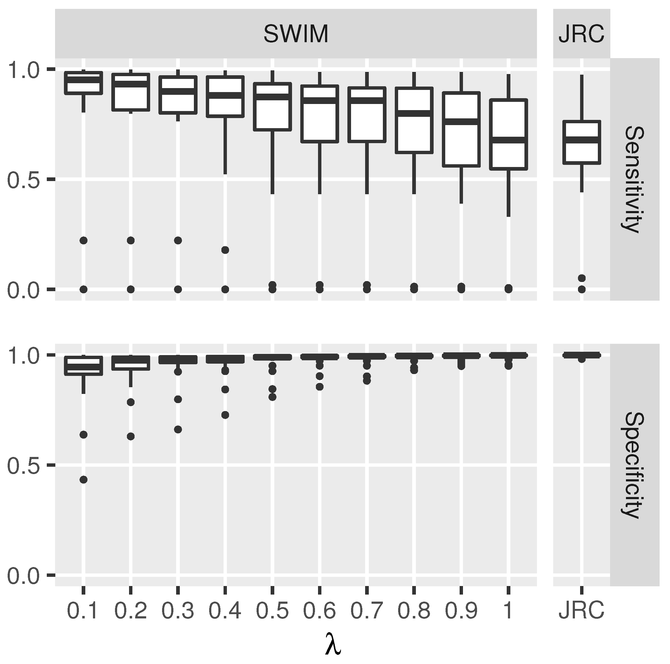
Figure 2 compares the JRC water classification sensitivity and specificity to those of the SWIM water classifications at various values of the tuning parameter λ . When λ = 1 , the SWIM classification framework is equivalent to training the random forest classifier using the JRC water classification labels alone, as it includes no extra information from the CBC algorithm. As λ decreases toward 0, more information from the clustering step is included in the training. It is evident that including the information from the clustering step is useful in increasing the sensitivity of the water classifications. As the sensitivity increases, there is a slight decrease in the specificity of the classifications, as expected, but the relative increase in sensitivity is of more value than the decrease in specificity, at least until λ is less than 0.3.
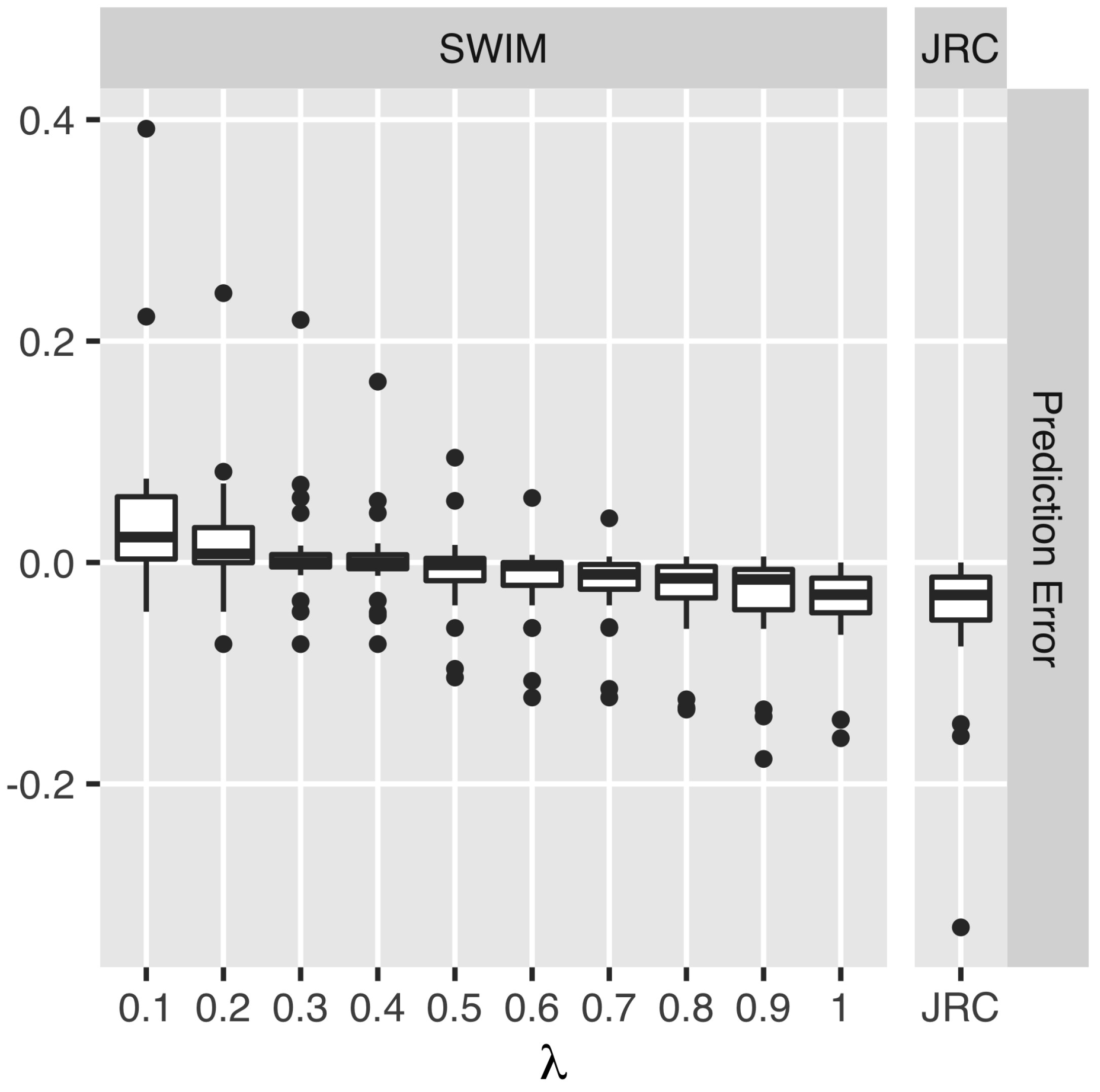
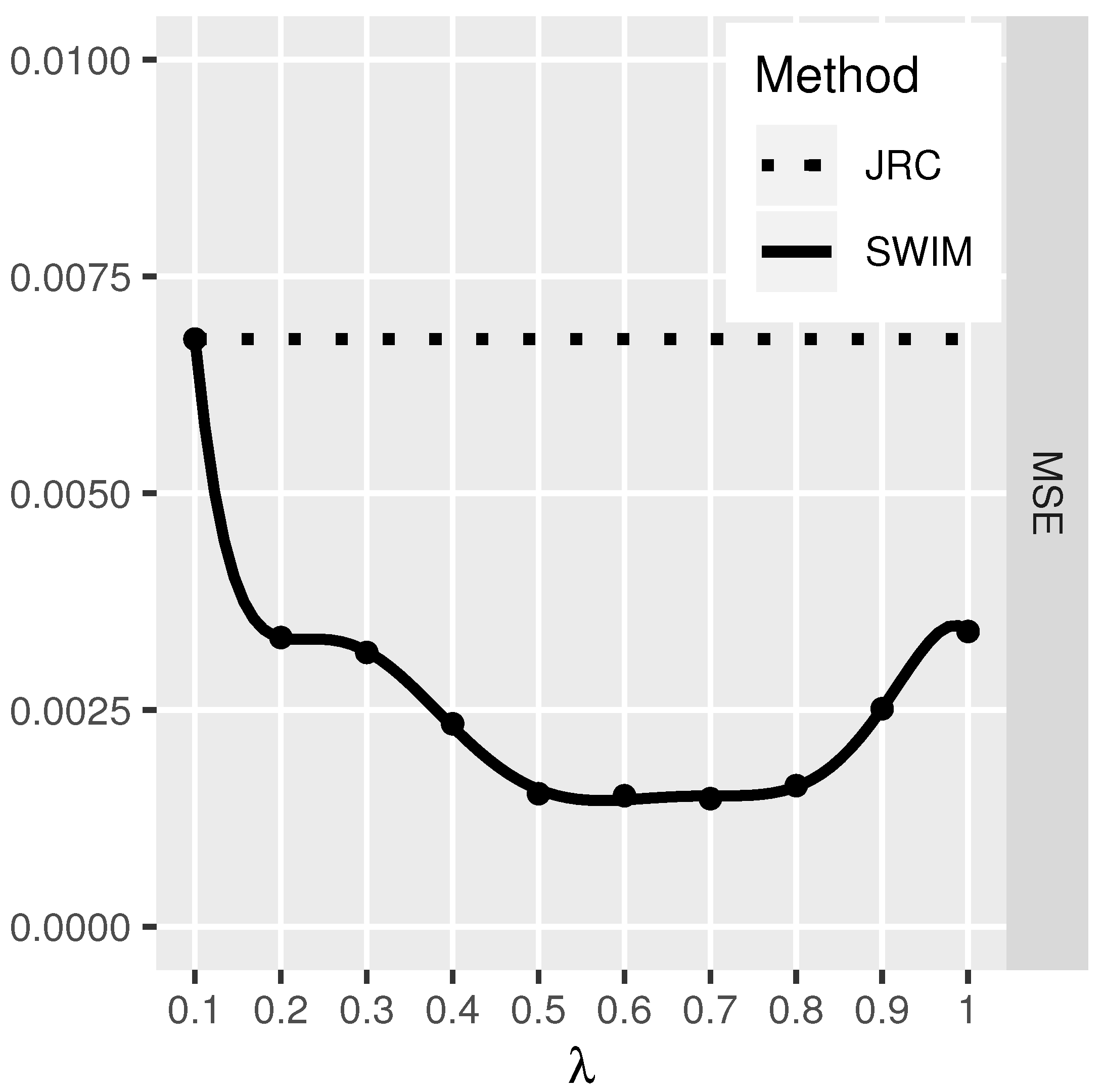
When comparing the error in the estimated water proportions ϵ JRC and ϵ SWIM as shown in Figure 3, we see that the JRC method has high negative bias compared to the SWIM classification framework. Using SWIM, the bias of the predicted water proportion approaches zero as the value of λ decreases to 0.5. On average, the bias of the JRC method is −0.0483, while the SWIM bias is smallest, 0.00317, at λ = 0.4 . Comparatively, the bias for the JRC method is more than 15 times greater than the SWIM bias at λ = 0.4 . The variance of the prediction errors using the SWIM classification framework is also generally less than the JRC method. Table 1 gives the average bias and standard deviation of the prediction errors for these methods. SWIM begins to significantly over-predict the total amount of water in these images as λ decreases past 0.3. The mean squared error (MSE) for the methods is presented in Figure 4. There is a robust reduction in MSE amongst the chosen level of λ in this validation study.
Given these statistics, a sensitivity analysis can be performed to select a value of λ . Mean prediction bias, as reported in Table 1, is absolutely minimal at λ = 0.4 . Similarly, the mean squared error of predicted proportion water versus validation proportion water is near its minimum at λ = 0.5 . The optimization of a simple mean of average sensitivity and specificity across the 27 validation ROI occurs at λ = 0.3 . In our validation study, this sensitivity analysis supports the selection of λ between 0.3 and 0.5 as an optimal value for the parameter.
Similarly, a sensitivity analysis may be performed to select a value of λ to use for new ROI, but the above results may also be taken into account without having to conduct a formal analysis. Our analysis suggests λ = 0.5 is a good starting value for most ROI. For some locations, decreasing the value of λ further increases the sensitivity of the method without significantly reducing the specificity. It seems reasonable to run the classifications at λ = 0.3 or λ = 0.1 and examine the spatial patterns of the classifications with previous intuition of the ROI, to see if the method seems to be over predicting the amount of water. It is possible that in some cases, a low value of λ may be more useful than λ = 0.5 . In any case, the SWIM outlier detection method will remove images that result in classifications that are suspect for over or under-prediction of total water.
This validation study offers convincing evidence that SWIM can produce water classifications that result in better sensitivity and estimation of waterbody extent than the JRC Monthly Water History dataset. The SWIM classification framework is useful for analyzing small to medium-sized waterbodies. The JRC method is better suited for global or large scale studies where precise identification of small areas of water is not important. As we have demonstrated, the SWIM classifications will help to identify areas in small waterbodies and wetlands that are also water-covered but not classified by the JRC method. For more precise monitoring of waterbodies of interest, it would be wise to utilize the SWIM classification framework.

3.2. New Orleans Case Study

The Bonnet-Carre Spillway near New Orleans, Louisiana, is opened when the Mississippi River floods to a level where excess water needs to be drained rapidly into Lake Pontchartrain. As of 2014, there are official records of the spillway being opened in at least 1994, 1997, 2008, and 2011 [38,39]. Within the spillway, there are also several semi-permanent small waterbodies which fluctuate seasonally. In this case study, we compare the ability of the JRC and SWIM classifications to accurately depict the dynamic nature of the surface water in this area, especially with regard to the occasional use of the spillway to drain floodwaters.
A four square mile region along the Mississippi River including the Bonnet-Carre Spillway was selected as the ROI for this case study. Using SWIM, we collected all Landsat images of this ROI between DOY 1 and 365 from 1984 to 2018, for a total of 884 images. The outlier detection step removed 59 images from the analysis.
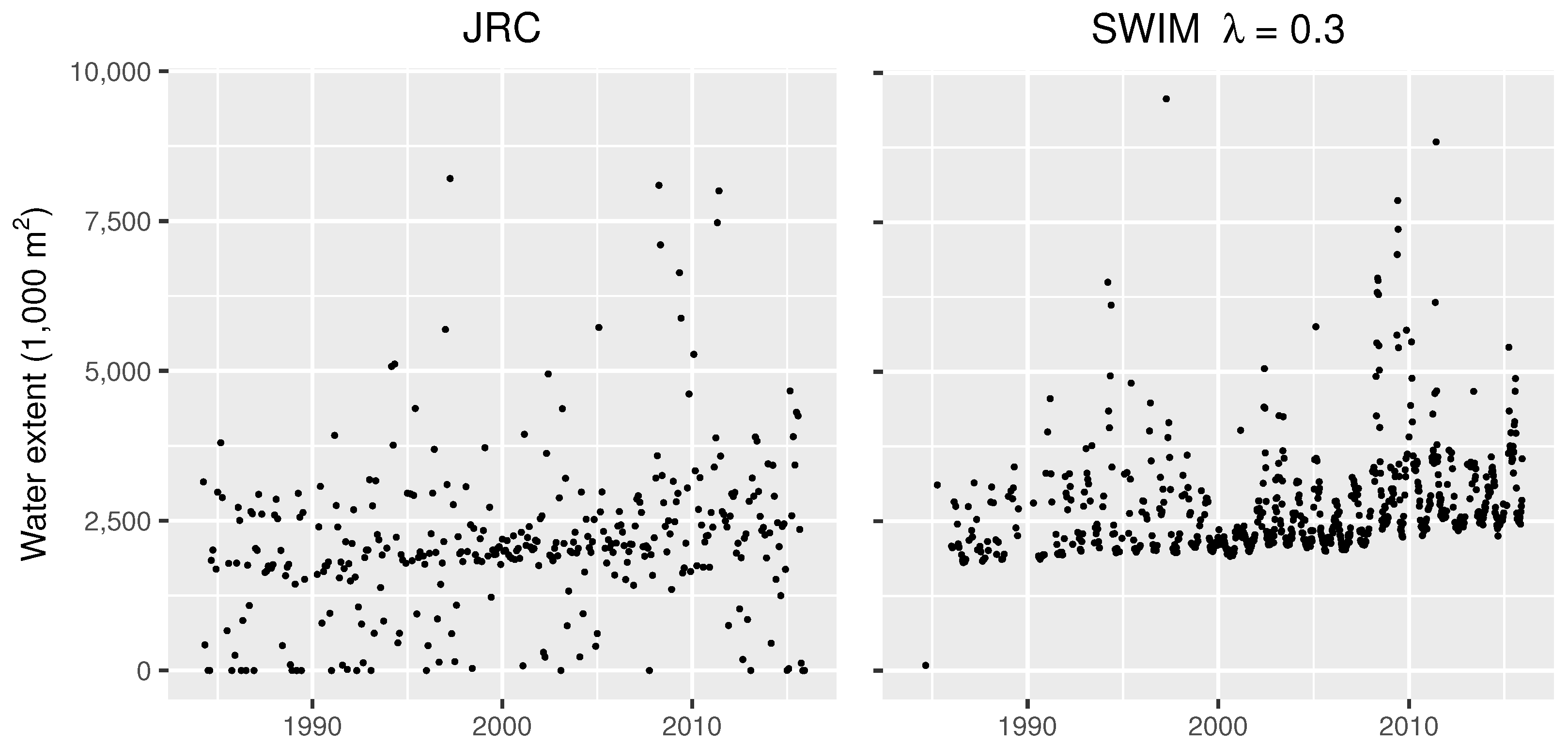
When comparing the JRC and SWIM classifications, the time series of total water extent (Figure 5) shows that the JRC dataset often greatly under-classifies the total water extent in this ROI. The time series generated from the SWIM classifications shows that the total extent of the water in the region is consistently greater than 1.5 million m 2 . The estimation of total water extent when using the JRC dataset is inaccurate due to the presence of missing classifications. This problem is remedied by using the SWIM classification framework to gap-fill missing data in all Landsat imagery. Furthermore, a more obvious seasonal trend within each year is evident in the SWIM time series.
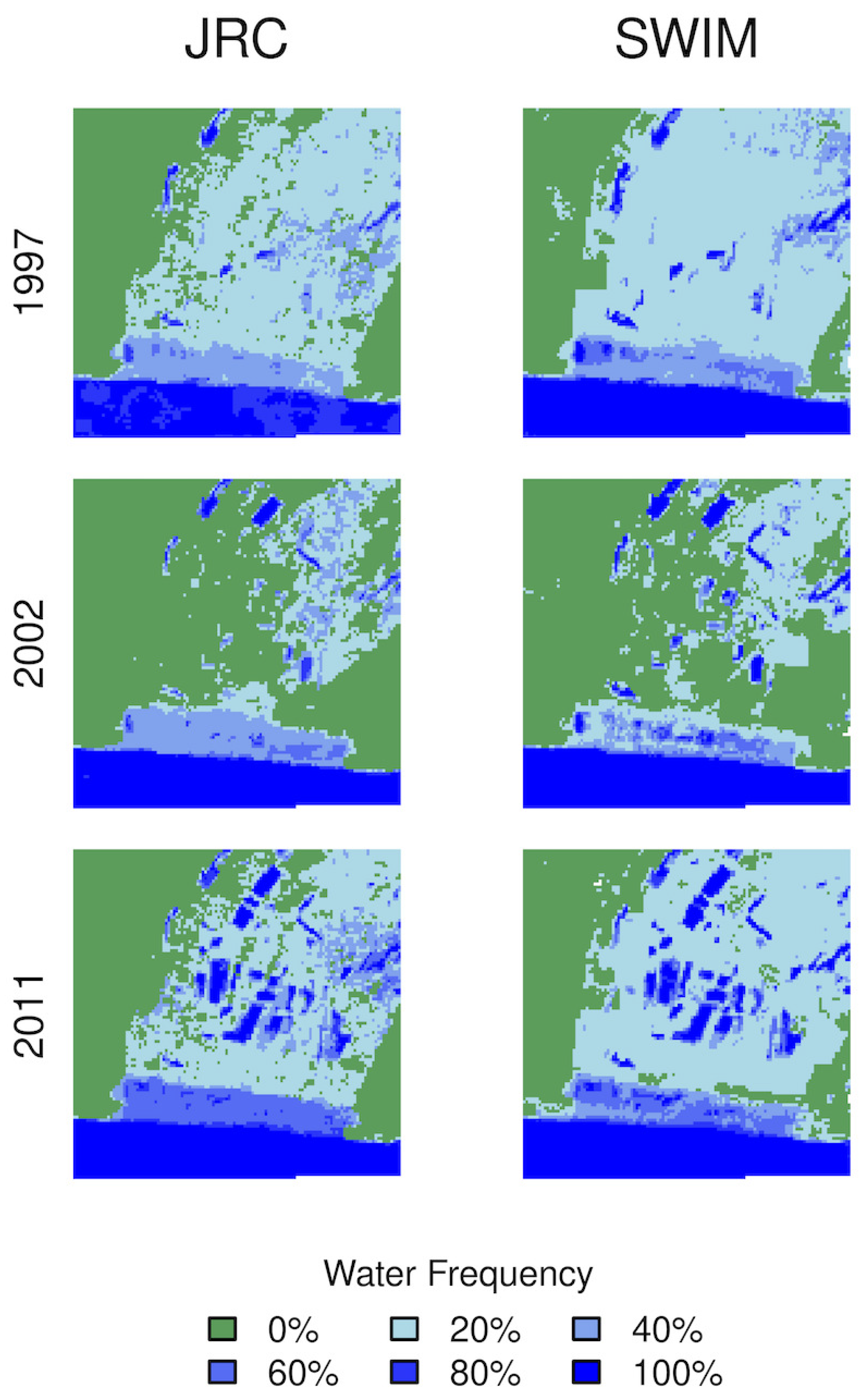
The SWIM outlier detection method retained many images with extremely high water extent. Upon inspection, it seems most of these images were captured on dates when the Bonnet-Carre spillway was open and draining floodwaters to Lake Pontchartrain. The SWIM classification framework accurately captures the floodwaters draining into the spillway in these years without removing these extreme events as outliers. Furthermore, the spatial representation of the classifications in Figure 6 show that SWIM increases sensitivity to surface water in the flooded spillway compared to the JRC dataset, complementing the results of the validation study. In years when the Bonnet-Carre Spillway was not open, such as in 2002, the SWIM classification framework also produces a more accurate estimation of the seasonal presence of the semi-permanent waterbodies within the spillway.

3.3. Devils Lake Case Study

Devil’s Lake in North Dakota has grown rapidly over the last 30 years. As the lake has grown it has destroyed the property and livelihood of many farmers [40]. The region we have selected for this case study is located near Minnewaukan, ND, a town that now finds itself on the edge of Devil’s Lake. The submonthly surface water classifications produced using SWIM outperform the JRC classifications in this ROI.
We selected a four square mile ROI along the edge of Devil’s Lake near Minnewaukan, ND. Using SWIM, we collected all Landsat images of this ROI between DOY 120 and 300 from 1984 to 2018, for a total of 1298 images. The outlier detection step removed 140 images from the analysis.
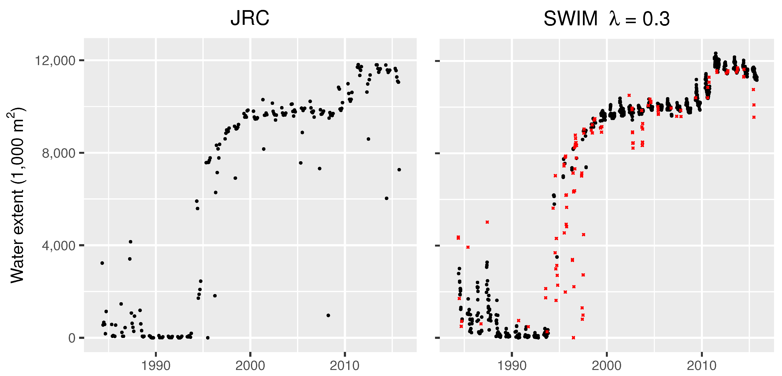
Many of the identified outliers were those which occurred during the rapid expansion of the lake between 1992 and 1996. In these images, the imputation algorithm did not perform reliably due to the rapidly changing water extent, which resulted in many of the imputed images being flagged as outliers. To illustrate the impact of the outlier detection step, the identified outliers are shown as crosses in Figure 7 for this case study. In the years before and after the rapid expansion of the lake, however, both the imputation and outlier detection methods perform reliably. The outlier detection step correctly removes images with unusually high or low water extent, such as those in 2002, 2003, and 2015. These images often contain unmasked cloud cover or shadow within the original Landsat image.
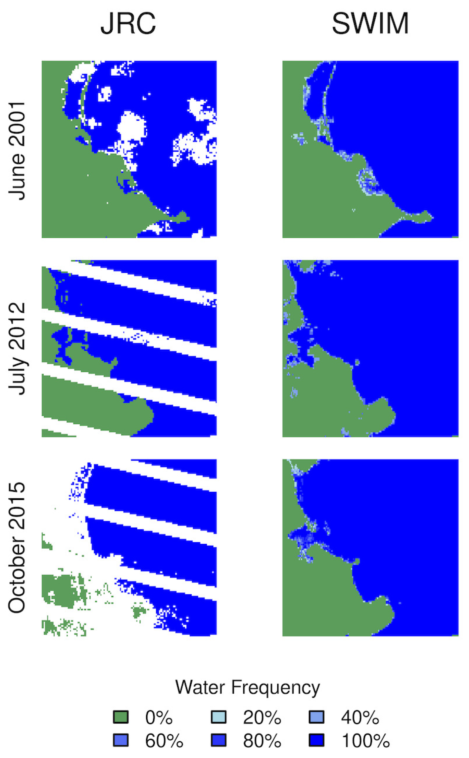
During years when the variability of the lake’s extent was mostly seasonal the SWIM classification framework’s reliance on imputation to produce multiple full classifications per month is an obvious advantage. Since the JRC dataset sometimes includes missing classifications, the estimation of total extent is occasionally much lower than expected. This can be seen in the time series of the JRC data (Figure 7), where some values fall much below the overall trend of total water extent in the ROI. This problem is remedied by gap-fill imputation in the SWIM classification framework (Figure 8). In October 2015, a large proportion of missing values occur in the JRC classification, while the SWIM method produces complete classifications for several images in this month. The SWIM classifications can show the within month variability of surface water in the ROI, which is especially evident in June 2001. In the SWIM results for this month we can see that a road in the upper-left quadrant of the image is surrounded by the lake and occasionally covered by water during this month. Eventually, the road is completely covered by water in subsequent years, as seen in the classification results for July 2012 and October 2015.

3.4. Colorado River Case Study

Extreme drought has occurred in the Colorado River Basin in recent years. Using the JRC Monthly Water History dataset for preliminary analyses, we selected a section of the Colorado River near White Canyon, Utah, which has greatly decreased in extent throughout this period of drought. In this case study, we compare the ability of the JRC and SWIM classifications to monitor the fluctuations in water extent due to drought in this region.
We selected a four square mile region of the Colorado River as the ROI for this case study. Using SWIM, we collected all Landsat images between DOY 120 and 300 from 1984 to 2018, for a total of 1111 images. The outlier detection step removed 105 images from the analysis.
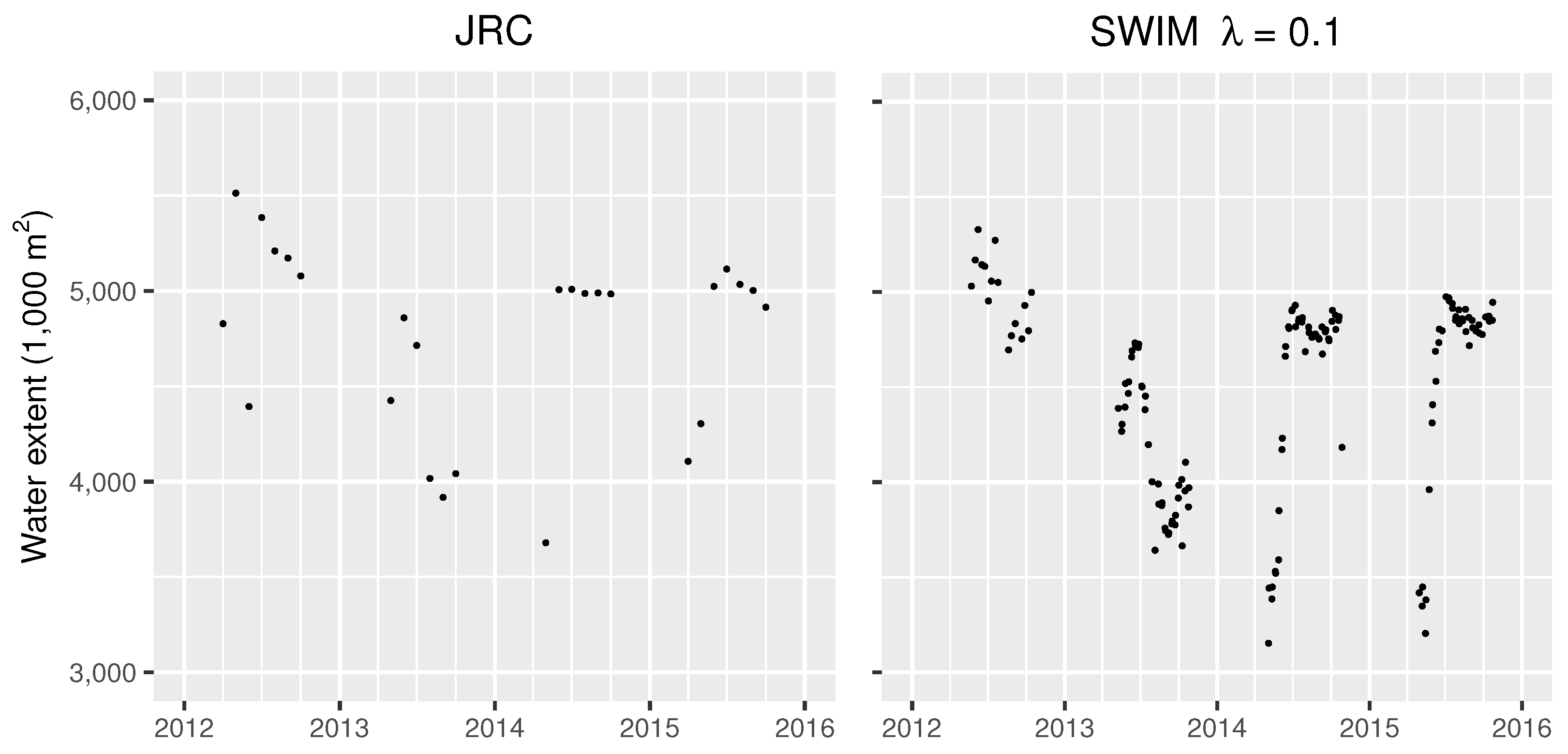
For this case study, we show a subset of the full time series of observations (Figure 9) in order to emphasize the SWIM classification framework’s high temporal resolution. It should be noted that a fair number of images with abnormally low total water extents were retained in the years after 2013, but these classifications upon further inspection, seem to accurately model the extreme drought that occurred in those years. The patterns in these images are similar to the water extents that occurred amongst other drought events and are therefore not removed as outliers.
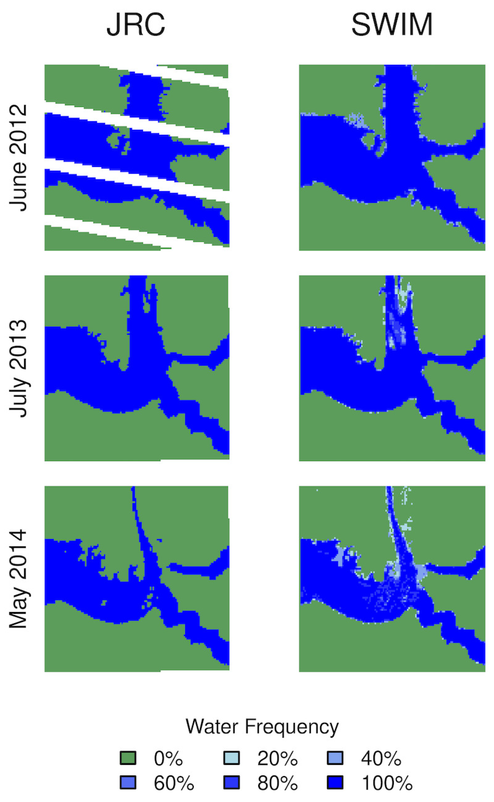
Compared to the JRC dataset, the submonthly SWIM classifications illustrate the surface water dynamics in the ROI at a much higher temporal resolution. This improvement can be used to monitor the spatial patterns of drought with greater detail (Figure 10). Imputation via SWIM allows a full estimation of the water extent in June 2012, whereas missing classifications are present in the JRC data. Areas of the river which were dry for only part of the month during July 2013 and May 2014 can be seen in the SWIM results but are not revealed by the JRC classifications. Furthermore, cyclical seasonal flooding and drought can be observed annually in this ROI using the SWIM classification framework, but is not evident in the JRC data. This case study shows that SWIM can be used to monitor surface water dynamics at the highest possible temporal resolution while utilizing Landsat imagery.

4. Discussion

The SWIM classification framework produces sensitive surface water classifications at submonthly frequency by gap-filling Landsat imagery. While the JRC Monthly Water History dataset provides global surface water classifications for each month, our study has shown that the JRC classifications have a negative bias for estimating the extent of small inland waterbodies and the monthly frequency is not adequate for thoroughly studying the impacts of short-term fluctuations and extreme weather events on these small waterbodies. The validation and case studies presented in this paper demonstrate that the SWIM classification framework outperforms the JRC dataset in classification analyses of small waterbody dynamics.
SWIM includes a series of methods to process and classify Landsat imagery. After using Google Earth Engine to efficiently pre-process and download the imagery, further analysis is conducted in R. The SWIM classification framework’s Cluster-based Bias Correction algorithm reduces classification bias compared to the JRC dataset by generating variations of "ground truth" training labels. Our validation study shows that this algorithm corrects for the negative bias of the JRC classifications by correctly classifying pixels as water under a variety of surface water conditions. SWIM then uses imputation to produce submonthly surface water classifications. This is an improvement compared to the JRC dataset, which produces monthly classifications after combining multiple Landsat images per month. Finally, to ensure the accuracy of the SWIM classification framework, our outlier detection method identifies images that may contain unmasked regions of cloud cover and random patches of incorrectly classified pixels. This step refines the analysis by filtering outliers from spatiotemporal representations of water extent.
Compared to previously available methods, the SWIM classification framework offers analysis of small waterbody dynamics with previously unattainable sensitivity and temporal frequency. For large regions, the JRC Monthly Water History dataset allows one to draw large scale conclusions about trends and extents. SWIM provides a more customizable experience that produces an analysis with the highest temporal resolution available from Landsat imagery. When taking care to ensure proper training of the random forest classifiers and reasonable imputation results, the SWIM classification framework can improve the sensitivity of the Landsat surface water classifications compared to the JRC classifications in many cases. However, the random forest classifiers apply only to the trained region of interest, compared to the JRC classification method, which applies to the entire globe. This trade-off between local and global applicability is a significant difference between the methods.
Steps for further improvement of SWIM are possible. The SWIM classification framework uses random forest classifiers, but state-of-the-art classification techniques such as segmentation via convolutional neural networks may produce more accurate results [41]. Including an expansive training dataset for such classifiers could expand the applicability of the method to larger regions and remove the requirement for localized training for each region of interest. We also intend to expand the range of satellite missions included in our sampling scheme for training data. Additionally, the SWIM classification framework’s imputation step is currently the computational limiting factor of this methodology. The computational efficiency of the STFIT method can be improved to allow our method to be applied to larger regions. This paper provides insight into the advantages of imputation for Landsat imagery and justifies the need for further investigation of such techniques. Finally, further validation of the SWIM classification framework could be performed to ensure classification accuracy across a variety of geographies outside of Iowa.
The case studies presented in this paper, however, show that the SWIM classification framework can provide valuable insight to small waterbody dynamics in a variety of applications. SWIM produces sub-monthly classifications by gap-filling each Landsat image via imputation to produce classifications for every image without any missing data. This allows one to predict the total water extent in an area at any observed time point in Landsat imagery, even if part or all of the original image contains cloud cover. This greatly increases the total time points available to assess water extent compared to once-per-month or seasonal analysis. This method can be used to assess the total surface water extent in a single Landsat image or in several images over a short period of time. Within a single month, it is possible that floodwaters could appear and disappear completely. Therefore sub-monthly classification is an important contribution and necessary for detailed surface water extent analysis. The New Orleans and Devil’s Lake case studies demonstrate the applicability of SWIM in flooded regions whereas the Colorado River case study demonstrates its performance during drought. In each of these case studies, the SWIM submonthly classifications provide enhanced understanding of each regions’ short-term trends and the spatial impact of extreme events. Given the results of these case studies, we are confident the SWIM classification framework outperforms the JRC dataset in the analysis of small waterbody dynamics.

5. Conclusions

In summary, the SWIM classification framework generates accurate, submonthly surface water classifications of Landsat imagery. We have achieved several novel and important contributions in this work. For small regions of interest that contain one or more inland waterbodies, SWIM can efficiently generate surface water classifications of every available Landsat image after imputing the missing values of masked pixels due to cloud cover, SLC failure, or other atmospheric effects. Cluster-based Bias Correction increases the sensitivity of our random forest classifiers to a variety of surface water conditions in local regions compared to the JRC Monthly Water History dataset. Finally, an outlier detection method identifies images that contain anomalous regions of classification errors prior to including these results in the final output. Given these contributions, the time series and spatial visualizations generated from the SWIM classification framework can represent the spatiotemporal dynamics of small inland waterbodies at previously unattainable sensitivity and temporal frequency.
The need to increase the sensitivity and temporal frequency of surface water classifications was our motivation for this study. The SWIM classification framework achieves this goal by producing reliable, sensitive, and consistent estimation of submonthly surface water extent. This has been achieved by gap-fill imputation to facilitate classification of all pixels in every available Landsat image. We believe the submonthly classification frequency of our framework will be of interest to other researchers who need to determine changes in water extent over short periods of time. Compared to the monthly period between JRC classifications, which may fail to capture the change of extent in waterbodies that occurs within each month, the SWIM framework achieves better analysis of waterbodies prone to short-term periods of flooding and drought. Our framework may be of use to those assessing the impact of extreme weather events, such as heavy rain storms and hurricanes. There is potential for further research and development of the SWIM framework, including the utilization of deep learning methods, increasing the computational efficiency of imputation, and expanding the training dataset sampling scheme to facilitate classification of large regions. In its current form, however, we are confident the SWIM classification framework can provide enhanced understanding of small waterbody dynamics given its submonthly classification frequency and local sensitivity to a variety of surface water conditions.

Author Contributions

Conceptualization, C.L., Z.Z. and Y.Z.; methodology, C.L. and Z.Z.; formal analysis, C.L. and X.C.; writing—original draft preparation, C.L. and X.C.; writing—review and editing, C.L., Z.Z., Y.Z.; supervision, Z.Z.; funding acquisition, Z.Z. All authors have read and agreed to the published version of the manuscript.

Funding

This research was supported in part by cooperative agreement 68-7482-17-009 between the USDA Natural Resources Conservation Service and Iowa State University and the National Science Foundation under Grant No. DGE-1828942.

Institutional Review Board Statement

Not applicable.

Informed Consent Statement

Not applicable.

Data Availability Statement

A GitHub repository (https://github.com/labuzzetta/swim, accessed on 28 April 2021) contains the code, examples, and validation data to reproduce the findings of this study. The SWIM framework is presented as a series of Google Earth Engine and R scripts to support additional analyses.

Conflicts of Interest

The authors declare no conflict of interest.

Appendix A. Masking Landsat Data

The Landsat 5 and 7 satellites provide ’sr_cloud_qa’ and ’pixel_qa’ quality information for each pixel. Landsat 8 provides similar ’sr_aerosol’ and ’pixel_qa’ values. The Landsat 5 and 7 missions use LEDAPS to assess pixel quality and provide bit values for general classifications including dense dark vegetation, cloud, cloud shadow, adjacent to cloud, snow, and water via the sr_cloud_qa band [42]. The Landsat 8 mission uses the LaSRC method and similarly reports bit values indicating fill (missing), aerosol retrieval, water, cloud or cirrus, cloud shadow, aerosol content [43].
SWIM uses the quality information from all three methods. Pixels with high-quality scores are retained, while pixels with other values are removed and imputed by the STFIT algorithm [30]. Pixels that are not removed for imputation must have one of the following high-quality scores in each quality band:
  • pixel_qa: 66, 68, 130, 132, 322, 324, 386, 388, 834, 836, 898, 900, 1346, 1348
  • sr_cloud_qa: 1, 32
  • sr_aerosol: 1, 2, 4, 32, 66, 68, 96, 100, 130, 132, 160, 164, 194, 224, 228

References

  1. NASA. Earth System Science Data Resources; National Aeronautics and Space Administration (NASA): Greenbelt, MD, USA, 2011.
  2. Friedl, M.; McIver, D.; Hodges, J.; Zhang, X.; Muchoney, D.; Strahler, A.; Woodcock, C.; Gopal, S.; Schneider, A.; Cooper, A.; et al. Global land cover mapping from MODIS: Algorithms and early results. Remote Sens. Environ. 2002, 83, 287–302. [Google Scholar] [CrossRef]
  3. Homer, C.; Huang, C.; Yang, L.; Wylie, B.; Coan, M. Development of a 2001 National Land-Cover Database for the United States. Photogramm. Eng. Remote Sens. 2004, 70, 829–840. [Google Scholar] [CrossRef] [Green Version]
  4. Pekel, J.F.; Cottam, A.; Gorelick, N.; Belward, A.S. High-resolution mapping of global surface water and its long-term changes. Nature 2016, 540, 418. [Google Scholar] [CrossRef]
  5. Guo, M.; Li, J.; Sheng, C.; Xu, J.; Wu, L. A review of wetland remote sensing. Sensors 2017, 17, 777. [Google Scholar] [CrossRef] [Green Version]
  6. Wulder, M.A.; White, J.C.; Loveland, T.R.; Woodcock, C.E.; Belward, A.S.; Cohen, W.B.; Fosnight, E.A.; Shaw, J.; Masek, J.G.; Roy, D.P. The global Landsat archive: Status, consolidation, and direction. Remote Sens. Environ. 2016, 185, 271–283. [Google Scholar] [CrossRef] [Green Version]
  7. Huang, C.; Chen, Y.; Zhang, S.; Wu, J. Detecting, extracting, and monitoring surface water From space using optical sensors: A review. Rev. Geophys. 2018, 56, 333–360. [Google Scholar] [CrossRef]
  8. Feng, M.; Sexton, J.O.; Channan, S.; Townshend, J.R. A global, high-resolution (30-m) inland water body dataset for 2000: First results of a topographic–spectral classification algorithm. Int. J. Digit. Earth 2016, 9, 113–133. [Google Scholar] [CrossRef] [Green Version]
  9. Mueller, N.; Lewis, A.; Roberts, D.; Ring, S.; Melrose, R.; Sixsmith, J.; Lymburner, L.; McIntyre, A.; Tan, P.; Curnow, S.; et al. Water observations from space: Mapping surface water from 25years of Landsat imagery across Australia. Remote Sens. Environ. 2016, 174, 341–352. [Google Scholar] [CrossRef] [Green Version]
  10. Rokni, K.; Ahmad, A.; Selamat, A.; Hazini, S. Water feature extraction and change detection using multitemporal Landsat imagery. Remote Sens. 2014, 6, 4173–4189. [Google Scholar] [CrossRef] [Green Version]
  11. Verpoorter, C.; Kutser, T.; Tranvik, L. Automated mapping of water bodies using Landsat multispectral data. Limnol. Oceanogr. Methods 2012, 10, 1037–1050. [Google Scholar] [CrossRef]
  12. Markham, B.; Storey, J.; Williams, D.; Irons, J. Landsat sensor performance: History and current status. IEEE Trans. Geosci. Remote Sens. 2004, 42, 2691–2694. [Google Scholar] [CrossRef]
  13. Feyisa, G.L.; Meilby, H.; Fensholt, R.; Proud, S.R. Automated Water Extraction Index: A new technique for surface water mapping using Landsat imagery. Remote Sens. Environ. 2014, 140, 23–35. [Google Scholar] [CrossRef]
  14. Isikdogan, F.; Bovik, A.C.; Passalacqua, P. Surface water mapping by deep learning. IEEE J. Sel. Top. Appl. Earth Obs. Remote Sens. 2017, 10, 4909–4918. [Google Scholar] [CrossRef]
  15. Gorelick, N.; Hancher, M.; Dixon, M.; Ilyushchenko, S.; Thau, D.; Moore, R. Google Earth Engine: Planetary-scale geospatial analysis for everyone. Remote Sens. Environ. 2017. [Google Scholar] [CrossRef]
  16. Foga, S.; Scaramuzza, P.L.; Guo, S.; Zhu, Z.; Dilley, R.D.; Beckmann, T.; Schmidt, G.L.; Dwyer, J.L.; Hughes, M.J.; Laue, B. Cloud detection algorithm comparison and validation for operational Landsat data products. Remote Sens. Environ. 2017, 194, 379–390. [Google Scholar] [CrossRef] [Green Version]
  17. Du, Z.; Li, W.; Zhou, D.; Tian, L.; Ling, F.; Wang, H.; Gui, Y.; Sun, B. Analysis of Landsat-8 OLI imagery for land surface water mapping. Remote Sens. Lett. 2014, 5, 672–681. [Google Scholar] [CrossRef]
  18. Fisher, A.; Flood, N.; Danaher, T. Comparing Landsat water index methods for automated water classification in eastern Australia. Remote Sens. Environ. 2016, 175, 167–182. [Google Scholar] [CrossRef]
  19. Ji, L.; Zhang, L.; Wylie, B. Analysis of dynamic thresholds for the Normalized Difference Water Index. Photogramm. Eng. Remote Sens. 2009, 75, 1307–1317. [Google Scholar] [CrossRef]
  20. Gao, B. NDWI-A normalized difference water index for remote sensing of vegetation liquid water from space. Remote Sens. Environ. 1996, 58, 257–266. [Google Scholar] [CrossRef]
  21. McFeeters, S.K. The use of the Normalized Difference Water Index (NDWI) in the delineation of open water features. Int. J. Remote Sens. 1996, 17, 1425–1432. [Google Scholar] [CrossRef]
  22. Xu, H. Modification of normalised difference water index (NDWI) to enhance open water features in remotely sensed imagery. Int. J. Remote Sens. 2006, 27, 3025–3033. [Google Scholar] [CrossRef]
  23. Frazier, P.S.; Page, K.J. Water body detection and delineation with Landsat TM data. Photogramm. Eng. Remote Sens. 2000, 66, 1461–1467. [Google Scholar]
  24. Pelleg, D.; Moore, A.W. X-means: Extending K-means with efficient estimation of the number of clusters. In Proceedings of the Seventeenth International Conference on Machine Learning, Stanford, CA, USA, 29 June–2 July 2000; pp. 727–734. [Google Scholar]
  25. Breiman, L. Random forests. Mach. Learn. 2001, 45, 5–32. [Google Scholar] [CrossRef] [Green Version]
  26. Chen, J.; Zhu, X.; Vogelmann, J.E.; Gao, F.; Jin, S. A simple and effective method for filling gaps in Landsat ETM+ SLC-off images. Remote Sens. Environ. 2011, 115, 1053–1064. [Google Scholar] [CrossRef]
  27. Yin, G.; Mariethoz, G.; Sun, Y.; McCabe, M.F. A comparison of gap-filling approaches for Landsat-7 satellite data. Int. J. Remote Sens. 2017, 38, 6653–6679. [Google Scholar] [CrossRef]
  28. Zeng, C.; Shen, H.; Zhang, L. Recovering missing pixels for Landsat ETM + SLC-off imagery using multi-temporal regression analysis and a regularization method. Remote Sens. Environ. 2013, 131, 182–194. [Google Scholar] [CrossRef]
  29. Zhu, X.; Liu, D.; Chen, J. A new geostatistical approach for filling gaps in Landsat ETM+ SLC-off images. Remote Sens. Environ. 2012, 124, 49–60. [Google Scholar] [CrossRef]
  30. Zhu, W. Topics in Sparse Functional Data Analysis. Ph.D. Dissertation, Iowa State University, Ames, IA, USA, 2018. [Google Scholar]
  31. Yao, F.; Wang, J.; Wang, C.; Cretaux, J. Constructing long-term high-frequency time series of global lake and reservoir areas using Landsat imagery. Remote Sens. Environ. 2019, 232, 111210. [Google Scholar] [CrossRef]
  32. Yao, F.; Müller, H.G.; Wang, J.L. Functional data analysis for sparse longitudinal data. J. Am. Stat. Assoc. 2005, 100, 577–590. [Google Scholar] [CrossRef]
  33. Liaw, A.; Wiener, M. Classification and regression by randomForest. R News 2002, 2, 18–22. [Google Scholar]
  34. Vuolo, F.; Ng, W.T.; Atzberger, C. Smoothing and gap-filling of high resolution multi-spectral time series: Example of Landsat data. Int. J. Appl. Earth Obs. Geoinf. 2017, 57, 202–213. [Google Scholar] [CrossRef]
  35. Maechler, M.; Rousseeuw, P.; Croux, C.; Todorov, V.; Ruckstuhl, A.; Salibian-Barrera, M.; Verbeke, T.; Koller, M.; Conceicao, E.L.T.; Anna di Palma, M. Robustbase: Basic Robust Statistics. R package version 0.93-7. 2021. Available online: http://robustbase.r-forge.r-project.org/ (accessed on 22 March 2021).
  36. Geoffrey Gabbott, W. National Agriculture Imagery Program (NAIP); United States Department of Agriculture Farm Service Agency Aerial Photography Field Office: Salt Lake City, UT, USA, 2010. [Google Scholar]
  37. USGS. National Hydrography Geodatabase; United States Geological Survey (USGS): Washington, DC, USA, 2013.
  38. Lane, R.R.; Day, J.W.; Kemp, G.; Demcheck, D.K. The 1994 experimental opening of the Bonnet Carre Spillway to divert Mississippi River water into Lake Pontchartrain, Louisiana. Ecol. Eng. 2001, 17, 411–422. [Google Scholar] [CrossRef]
  39. U.S. Army Corps of Engineers. Bonnet Carre Spillway; US Army Corps of Engineers New Orleans District: Norco, LA, USA, 2014.
  40. Todhunter, P.E.; Rundquist, B.C. Terminal lake flooding and wetland expansion in Nelson County, North Dakota. Phys. Geogr. 2004, 25, 68–85. [Google Scholar] [CrossRef]
  41. Yu, L.; Wang, Z.; Tian, S.; Ye, F.; Ding, J.; Kong, J. Convolutional neural networks for water body extraction from Landsat imagery. Int. J. Comput. Intell. Appl. 2017, 16, 1750001. [Google Scholar] [CrossRef]
  42. Masek, J.; Vermote, E.; Saleous, N.; Wolfe, R.; Hall, F.; Huemmrich, K.; Gao, F.; Kutler, J.; Lim, T. LEDAPS Landsat Calibration, Reflectance, Atmospheric Correction Preprocessing Code; Oak Ridge National Laboratory Distributed Active Archive Center: Oak Ridge, TN, USA, 2012. [Google Scholar]
  43. Vermote, E.; Roger, J.C.; Franch, B.; Skakun, S. LaSRC (Land Surface Reflectance Code): Overview, application and validation using MODIS, VIIRS, Landsat and Sentinel 2 data’s. In Proceedings of the IEEE International Geoscience and Remote Sensing Symposium, Valencia, Spain, 22–27 July 2018; pp. 8173–8176. [Google Scholar] [CrossRef] [Green Version]
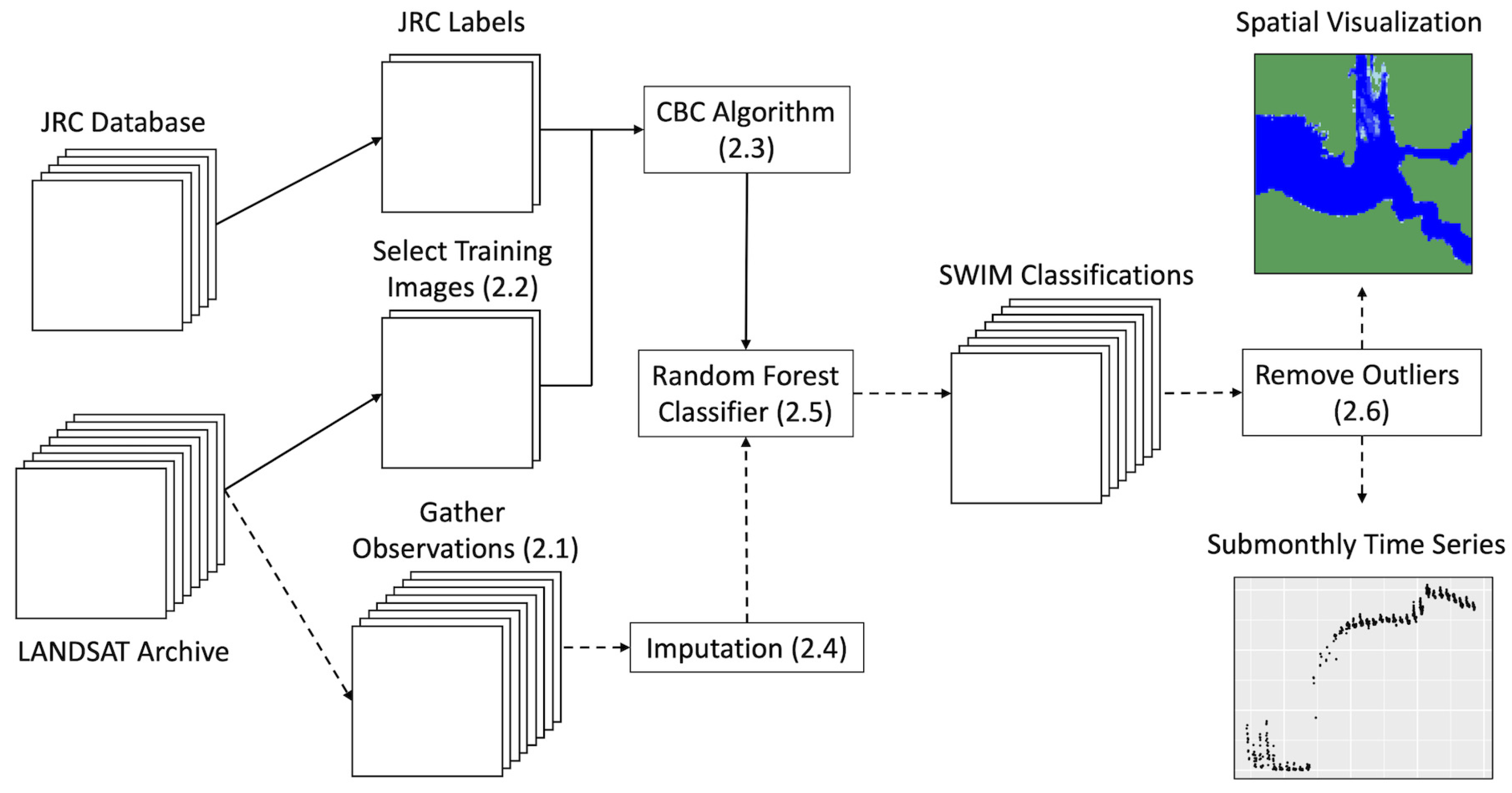
Figure 1. Visual summary of the SWIM classification framework. The relevant sections of this paper are listed in parentheses, e.g., (2.1).
Remotesensing 13 01742 g001
Figure 2. The sensitivity and specificity of the JRC and SWIM classifications using various levels of λ for 27 ROI sampled from the National Hydrography Dataset in Iowa. Classification sensitivity and specificity is calculated at the pixel level for each validation ROI by comparing pixel classifications to high resolution National Agriculture Imagery Program 1 m resolution images taken within the same month as the sampled Landsat image.
Remotesensing 13 01742 g002
Figure 3. Prediction error based on predicted proportion water versus validated proportion water in 27 validation ROI for the JRC and SWIM classifications using various levels of λ .
Remotesensing 13 01742 g003
Figure 4. Mean squared error of predicted proportion water versus validated proportion water in 27 validation ROI for the JRC and SWIM classifications using various levels of λ .
Remotesensing 13 01742 g004
Figure 5. Time series of total estimated water extent in New Orleans ROI using the JRC dataset and SWIM classification framework at λ = 0.3 . The data are plotted for all available time-points for each method between 1 January 1984 and 31 December 2015.
Remotesensing 13 01742 g005
Figure 6. Spatial representation of water extent frequency in New Orleans ROI for three separate years of JRC and SWIM classifications, including all available time-points for each method in the years 1997, 2002, and 2011.
Remotesensing 13 01742 g006
Figure 7. Time series of total estimated water extent in Devil’s Lake ROI using the JRC dataset and SWIM classification framework at λ = 0.3 . The data are plotted for all available time-points for each method between 1 January 1984 and 31 December 2015. Images selected as outliers by SWIM are included in the plot and indicated by red crosses for this case study.
Remotesensing 13 01742 g007
Figure 8. Spatial representation of water extent frequency in Devil’s Lake ROI for three separate months of JRC and SWIM classifications, including all available time-points for each method in June 2001, July 2012, and October 2015.
Remotesensing 13 01742 g008
Figure 9. Time series of total estimated water extent in Colorado River ROI using the JRC dataset and SWIM classification framework at λ = 0.1 . The data are plotted for all available time-points for each method between 1 January 2012 and 31 December 2015.
Remotesensing 13 01742 g009
Figure 10. Spatial representation of water extent frequency in Colorado River ROI for three separate months of JRC and SWIM classifications, including all available time-points for each method in June 2012, July 2013, and May 2014.
Remotesensing 13 01742 g010
Table 1. Mean prediction bias and prediction error standard deviations reported for 27 validation ROI when using the JRC and SWIM pipeline classifications at various levels of λ .
MethodMeanStd Dev
JRC−0.048300.0679
SWIM λ = 1.0 −0.039600.0429
SWIM λ = 0.9 −0.034100.0456
SWIM λ = 0.8 −0.028500.0398
SWIM λ = 0.7 −0.019700.0345
SWIM λ = 0.6 −0.016900.0357
SWIM λ = 0.5 −0.008850.0381
SWIM λ = 0.4 0.003170.0410
SWIM λ = 0.3 0.009600.0502
SWIM λ = 0.2 0.021300.0554
SWIM λ = 0.1 0.045500.0845
Publisher’s Note: MDPI stays neutral with regard to jurisdictional claims in published maps and institutional affiliations.