Article

Assessing Spatial Variation in Algal Productivity in a Tropical River Floodplain Using Satellite Remote Sensing

1
Australian Rivers Institute, Griffith University, Nathan 4111, Australia
2
Coasts and Oceans Research Program, CSIRO Oceans and Atmosphere, Brisbane 4102, Australia
*
Author to whom correspondence should be addressed.
Remote Sens. 2021, 13(9), 1710; https://doi.org/10.3390/rs13091710
Submission received: 9 March 2021 / Revised: 20 April 2021 / Accepted: 26 April 2021 / Published: 28 April 2021

Abstract

:
Studies of tropical floodplains have shown that algae are the primary source material for higher consumers in freshwater aquatic habitats. Thus, methods that can predict the spatial variation of algal productivity provide an important input to better inform management and conservation of floodplains. In this study, a prediction of the spatial variability in algal productivity was made for the Mitchell River floodplain in northern Australia. The spatial variation of aquatic habitat types and turbidity were estimated using satellite remote sensing and then combined with statistical modelling to map the spatial variation in algal primary productivity. Open water and submerged plants habitats, covering 79% of the freshwater flooded floodplain extent, had higher rates of algal production compared to the 21% cover of emergent and floating aquatic plant habitats. Across the floodplain, the predicted average algal productivity was 150.9 ± 95.47 SD mg C m−2 d−1 and the total daily algal production was estimated to be 85.02 ± 0.07 SD ton C. This study provides a spatially explicit representation of habitat types, turbidity, and algal productivity on a tropical floodplain and presents an approach to map ‘hotspots’ of algal production and provide key insights into the functioning of complex floodplain–river ecosystems. As this approach uses satellite remotely sensed data, it can be applied in different floodplains worldwide to identify areas of high ecological value that may be sensitive to development and be used by decision makers and river managers to protect these important ecological assets.

Graphical Abstract

1. Introduction

Aquatic food webs on river floodplains depend on primary producers such as phytoplankton and epiphyton as the major basal food sources that support higher order consumers [1,2,3,4]. Because algae are such an important food resource for higher trophic levels in river systems [5], numerous studies across different ecosystems have developed methods to measure rates of production [6,7,8,9,10,11]. In general, estimating rates of algal production provides more information than algal biomass about ecosystem function, because observed biomass is the outcome of several processes [12]. Importantly, observed biomass represents what is left after losses due to consumption by invertebrates, whereas the rate of production represents the productivity of the base of the food web including the uptake of nutrients from the system [13]. As such, direct measurement of rates of algal production across inundated floodplains is important as it reflects the amount of carbon being produced per unit of time, which in turn supports the secondary production of aquatic consumers [14].
Such field-based measurements provide crucial information at local scales that can also be integrated into statistical models and combined with remote sensing data to predict algal productivity in new locations [9]. This can be particularly valuable in remote areas and for large floodplain systems where, field work can be constrained by logistical challenges limiting access during periods of inundation, but for which data from remote sensing methods may be available. In this way, field data can support remote sensing information, which can enable the estimation of rates of primary production at broader spatial scales [15].
Satellite remote sensing has become an important tool for enhancing spatial ecological modelling and mapping of algal primary productivity dynamics [6,16]. Such approaches have been successfully applied to directly estimate phytoplankton abundance and productivity in large inland open water areas [6,17,18,19] and in floodplains [20]. While studies on phytoplankton using remote sensing techniques are common, similar work focused on epiphyton productivity are not as widespread; but see [11]. The estimation of epiphyton dynamics through remote sensing is complicated by the aquatic macro-vegetation to which epiphyton is most commonly attached. While aquatic macro-vegetation stem and leaves provide habitat for epiphytic algae to grow [21,22], these structures also create a physical barrier for remote observation. To overcome this challenge, studies that have estimated epiphyton biomass and productivity using remote sensing, have generally combined field data with modelling approaches [11,20]. Given the importance of these primary producers to floodplain river ecology, methods to monitor spatial variation in algal productivity and identifying hotspots of production are needed to establish key areas for floodplain restoration and conservation.
This study builds upon a previous local, field-data-based statistical model developed to predict the spatial variation of algal productivity in the Mitchell River, northern Australia [9], aiming to expand its application to the floodplain scale by including satellite remotely sensed data. This previous research showed that turbidity and macrophyte cover, or its absence, could be used to predict rates of phytoplankton and epiphyte production with reasonable accuracy [9] and both of these predictor variables can be observed via remote sensing [20,23,24,25,26]. In this study, we use Landsat 8 images to remotely predict turbidity and macrophyte cover in order to facilitate algal productivity predictions across the Mitchell River floodplain. The ability to spatially extrapolate algal productivity to the landscape scale allows the identification of hotspots of production on the floodplain. The identification of floodplain areas where algal productivity might be higher can be used by river managers in order to prioritize those areas for preservation and to mitigate possible impacts of land and water resource development [27].

2. Materials and Methods
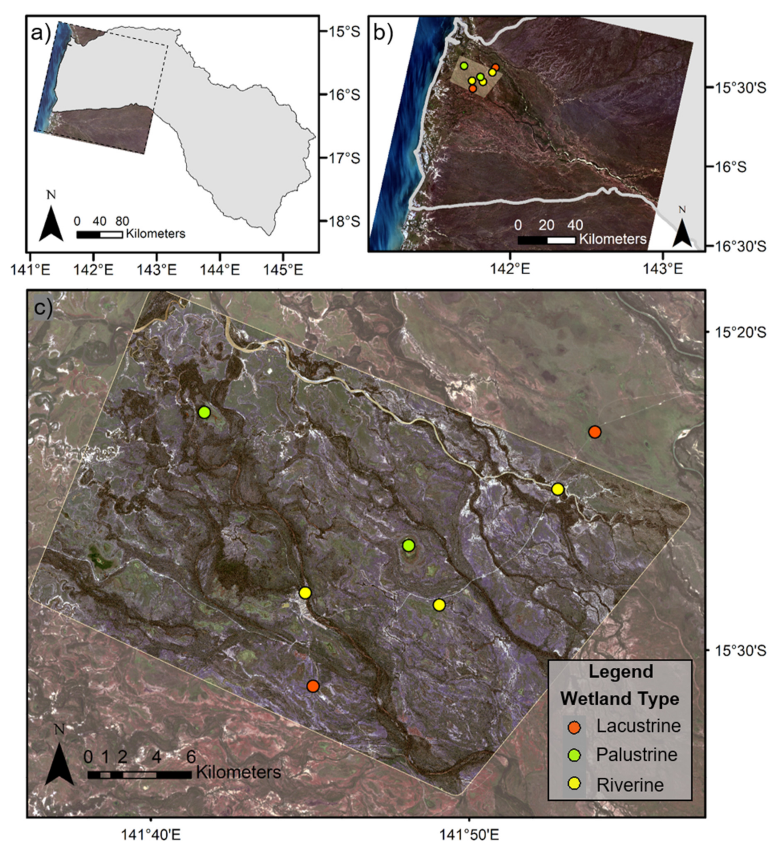
2.1. Study Area

Our study area is the Mitchell River floodplain, located in wet-dry tropical Queensland, Australia (Figure 1). This region has a strongly seasonal climate due to a monsoonal weather pattern. Most of the annual rainfall occurs during the wet season, between December and March, and the resulting runoff creates a vast inundated floodplain [28]. In 2018, the wet season was delayed and most of the rainfall and discharge at Dunbar gauging station happened between February and April (Figure A1).The Mitchell River floodplain supports a large number of off-stream wetlands [28], which in turn support aquatic macrophytes and algal production [9,25] thereby playing an important role in sustaining aquatic biodiversity. The catchments of tropical rivers in northern Australia, which includes the Mitchell River, have low levels of agricultural, urban, or water resource development compared with other regions of the country [29]. Nonetheless, a significant increase in agricultural development is proposed for the Mitchell River with subsequent water extraction from expanded water resource development [30]. The Mitchell River floodplain ecosystem provides a valuable case study because of the low levels of development in a highly complex system [31], which allowed the identification of key habitats of high ecological value in a relatively undisturbed ecosystem that is under pressure for further development [30].

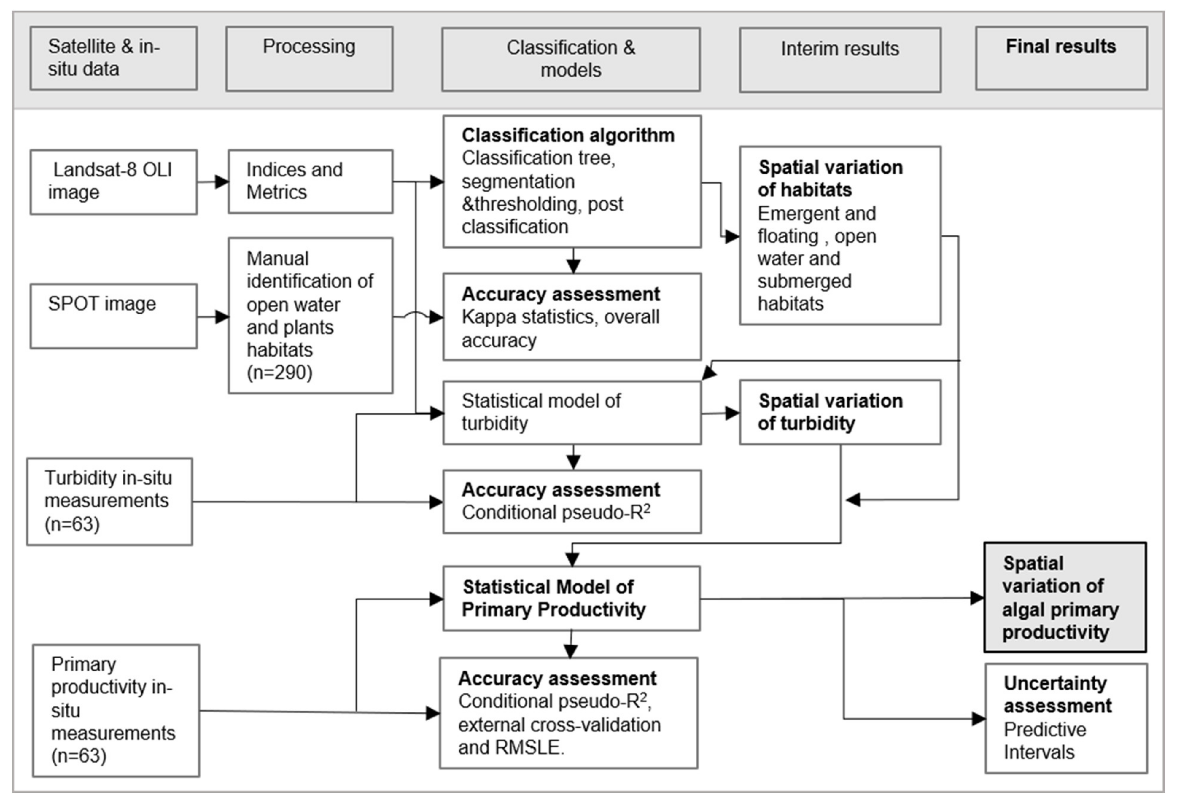
2.2. Methodological Framework

The methodological framework of this study was based on four steps: (1) data acquisition (satellite and in-situ data), (2) image processing, (3) classification and statistical modelling to spatially classify aquatic habitat types, estimate turbidity, and predict algal primary productivity variation across the Mitchell River floodplain, and (4) accuracy and uncertainty assessments (Figure 2). The satellite data used in this study were Landsat 8 and SPOT 7 imagery. Landsat 8 image band and index data (30 m resolution) were used as input to a classification tree algorithm to estimate the spatial variation in aquatic habitats and the statistical models to predict spatial variation in turbidity. The high-resolution (6 m) SPOT 7 image was used to assess the accuracy of the habitat classification. Rates of algal production across the floodplain were obtained via an additional statistical model that used predicted spatial variation in turbidity and habitat as inputs. In-situ data were obtained in a single sampling campaign conducted in April 2018 [9] and were used to calibrate and perform the accuracy assessments of the statistical models of turbidity and algal productivity. Additionally, predictive intervals were calculated for algal productivity predictions.

2.3. Data Acquisition

2.3.1. Field Campaign

A sampling campaign was conducted in late April 2018 at the end of the wet season while the wetlands were still largely inundated. Our sampling design included seven sites, comprising 3 riverine, 2 lacustrine, and 2 palustrine wetlands (Figure 3), and at each site four different habitats were defined according to their dominant macrophyte structure: emergent (23 samples), submerged (14 samples), floating (19 samples), and open water habitats (7 samples) [9,22].
For each habitat replicate (n = 63), turbidity, depth, rooted plant and algal biomass, and algal productivity were measured in situ (for a detailed description of the methods applied to measure turbidity, biomass, and productivity, refer to Molinari et al. [9]). The wetlands were in general shallow, ranging between 0.2 and 2.2 m depth, and had relatively low turbidities, with an average of 24.15 Nephelometric Turbidity Units (NTU). The observed data on epiphytes and phytoplankton productivity were determined from carbon uptake incubations using 13C-bicarbonate [8,32]. Algal productivity ranged between 0.2 and 1014.0 mg C m−2d−1, with an average productivity of 158.6 mg C m−2d−1.

2.3.2. Optical Imagery

We used cloud free Landsat 8 Operational Land Imager (OLI) and SPOT 7 imagery, obtained on 25 April 2018 while the field sampling campaign was being conducted (Table 1). A single Landsat 8 OLI scene, at 30m pixel resolution was required to cover the Mitchell River floodplain study area (Figure 3). The Landsat imagery was downloaded from the United States Geological Survey’s Earth Explorer website (http://earthexplorer.usgs.gov accessed on 24 September 2018), as level 1T processed scenes. The Landsat scene was converted to surface reflectance by the Joint Remote Sensing Centre of the Queensland Department of Environment and Science, which included atmospheric correction with a standard aerosol adjustment, bidirectional reflectance distribution function (BRDF) adjustment, and topographic normalization [33] corresponding to a Level 2 data product. The SPOT 7 high resolution image (6m resolution) consisted of a single image covering a smaller portion of the floodplain compared to the Landsat image (Figure 3). The SPOT image was supplied commercially by Ozius Pty Ltd ortho-rectified and pan-sharpened using the weighted Brovey technique [34], corresponding to a Level 3 data product.

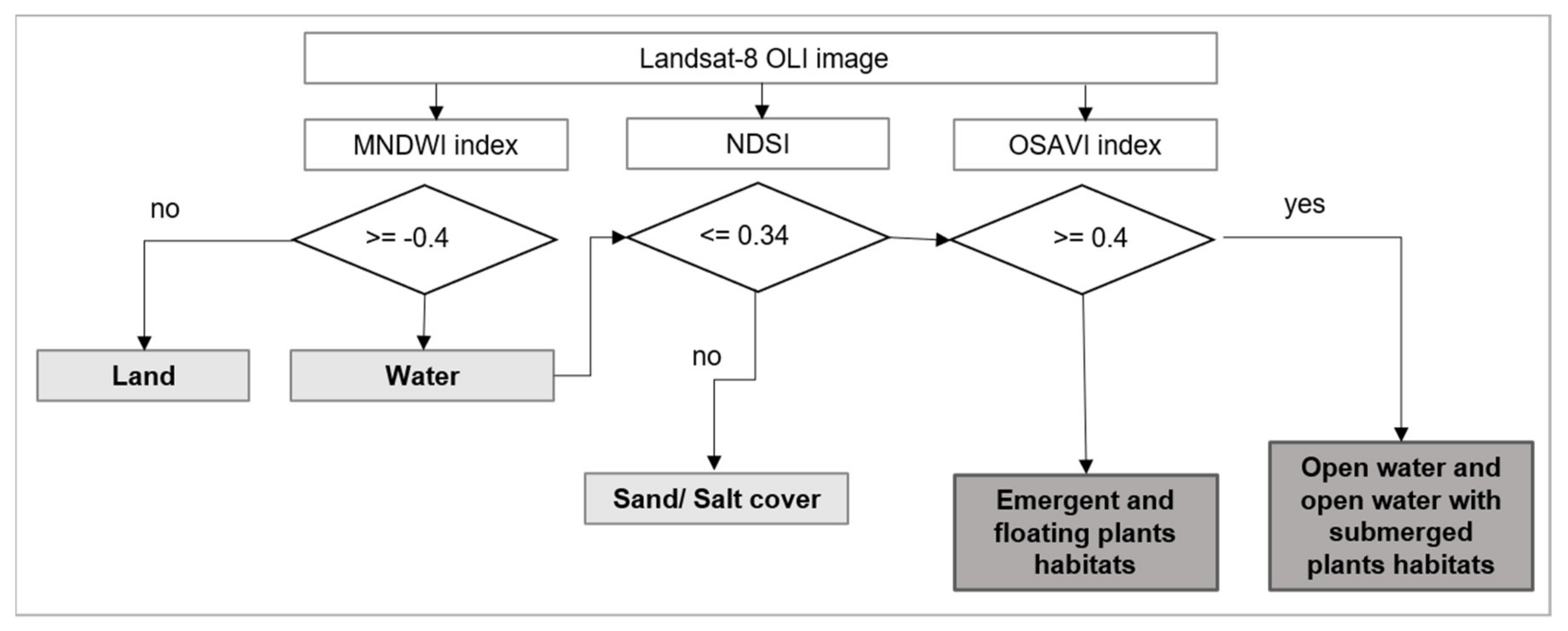
2.4. Statistical Modelling of Habitats

For the purpose of this study, remotely sensed habitats (from the Landsat 8 OLI and SPOT 7 images) were divided into two categories: (1) open water and open water with submerged plants (included in the same category due to difficulties in isolating the plant signatures from water column and substrate interference [26]), and (2) emergent and floating plant dominated habitats (included in the same category due to their similar spectral signatures [26]). Classification tree models [35] were applied to develop relationships between the habitat type and the predictor variables (spectral data and indices described below), using the rpart package [36] in the R statistical environment [37]. Classification tree models have been successfully applied to classify aquatic and other vegetation types from remotely sensed images [26,38,39,40].
Landsat 8 OLI visible and infrared bands and indices were tested as predictor variables to differentiate land cover, open water, and plant habitats. The visible and infrared indices tested were the automated water extraction index (AWEI), the normalized difference water index (NDWI), the modified NDWI (MNDWI), optimized soil adjusted vegetation index (OSAVI), and the normalized difference vegetation index (NDVI) (Table 2). These indices were selected for their usefulness in assessing wetland systems and dynamics in past studies; NDWI, MNDWI, and AWEI have been applied to map open water [41,42,43]. Additionally, MNDWI [44] was used to map flood inundation in Northern Australia [45]. OSAVI [46] and NDVI are common indices used to extract green biomass and vegetative coverage [47]. Recent studies using OSAVI showed that this index had greater accuracy than the most widely used NDVI [48]. The variable importance function in R was used to identify the key predictors guided by the explained variance [36].
We evaluated the classification performance of the decision tree algorithm by comparing the classification tree results to several accuracy points obtained from visual inspection of the SPOT 7 pan-sharpened image. Past studies have similarly validated classification performance using manually inspected SPOT images [45] and Google Earth imagery [40]. In total, 290 accuracy points, accounting for both habitat categories, open water and open water with submerged plants, and floating and emergent plants were randomly selected across the SPOT image extent to perform the validation of the classification of the Landsat Image. The number of accuracy points was chosen to account for at least 50 points on each habitat category [51]. We performed five times repeated k-fold cross validation (k = 5) by setting aside 60 observations and training the model on the remaining data [52]. The value of k was chosen given the size of the sample to avoid both high bias and variance [53]. We used each training model to predict habitat type on the Landsat image (fitted values) and repeated this process five times calculating the average rate between fitted and observed results. To estimate classification accuracy, we calculated the error of omission and commission and the percentage agreement (i.e., number of correctly classified sites/N).
Preliminary analysis of the Landsat image showed areas on the Mitchell River floodplain that were dominated by sand and saline plains that were mis-identified as very turbid water. The Mitchell River floodplain consists of large areas covered by sand or loam over sodic clay subsoils deriving from surficial alluvial sediments (i.e., deposited by rivers), and these areas are located as bed sands on the main rivers and closer to the coast [54]. There are also saline coastal marine plains, which were deposited during previous sea-level rises along the Gulf coast [54]. Those areas were re-analyzed and classified as sand/salt cover using the normalized difference sand index (NDSI) (Table 2) [49]. A 5 km buffer was applied around the coastal area because this part of the floodplain consists of large areas of salt pans with distinctly different rates of algal production [32]. The areas identified as sand or saline cover, and also the coastal buffered area, were excluded from the estimation of algal productivity in order to avoid extrapolation issues, given that we did not have observed data on those areas to support our model.

2.5. Statistical Modelling of Turbidity

To model turbidity, we used empirical statistical relationships between in situ measurements of turbidity and the spectral imagery captured by the satellites [55,56]. We included habitat type, estimates of total suspended matter (TSM) concentrations, and spectral information from the Landsat image as potential predictors of turbidity. Past studies have similarly used TSM [57] and habitat type [20] as predictor variables in statistical models of turbidity. For the spectral variables, we used the Landsat spectral bands and calculations of NDVI and NDWI (Table 2). The TSM concentrations were estimated using a semi-empirical algorithm developed for Australian inland waters, based on the relationship between the satellite-derived reflectance and the inherent optical properties of the water column (Table 2) [50]. This algorithm was previously used to access TSM across the catchments of northern Australia [45].
We used linear mixed-effect models to predict turbidity (lme4 package in R; [58]). Wetlands sites (n = 7) were considered as random intercepts to account for the multiple observations at each wetland [58]. For the fixed effects, the different Landsat bands and indices described above were tested as predictors in a model selection effort. The observed data consisted of 63 turbidity observations obtained during the field work, which were log-transformed to approximate normality and homoscedasticity. We selected the best fitting model based on Akaike’s Information Criterion (AIC) for goodness of fit [59] and to assess how well our model fitted the data we used the conditional pseudo-R2 [60]. The p-values for fixed effects of the model were calculated using the Kenward–Roger method (afex package in R; [61]).

2.6. Statistical Modelling of Algal Primary Productivity

For the prediction of algal primary productivity, we adapted the statistical model previously developed for Mitchell River floodplains [9]. This was a linear mixed-effects model, using turbidity and habitat type as fixed effects, and site as a random intercept to account for the multiple observations at each wetland [58]. The former model had four different categories of habitat type: emergent plants, floating plants, open water, and submerged plants. In this study, to adapt the model to the more spectrally limited remote sensing inputs, habitat type was limited to two categories: (1) Open water and open water with submerged plants; and (2) Emergent and Floating plants. We log-transformed the response variable and assessed how well our model fitted the data using the conditional pseudo-R2 [60]. To further test the average predictive performance of the model, we applied an external cross-validation [52] and measured the average correlation between predicted and observed data. Additionally, we measured the Root Mean Squared Logarithmic Error (RMSLE) [62]. The p-values for fixed effects of the model were calculated using the Kenward–Roger method (afex package in R; [61]).
To understand variations at the landscape scale, we calculated the mean, the standard deviation, and the sum of algal production in the wetlands across the floodplain and in the main rivers of the floodplain including the Mitchell, Alice, Scrutton, and Nassau Rivers (considering a buffer of 120m of each side of the streamline). To access the uncertainty of the predictions, we calculated the 95% predictive intervals for each prediction using the R package merTools [63]. Additionally, we calculated the approximate predictive interval of the total productivity, considering the predictions to be independent and taking the square root of the sum of the variance of each prediction [64,65].

3. Results

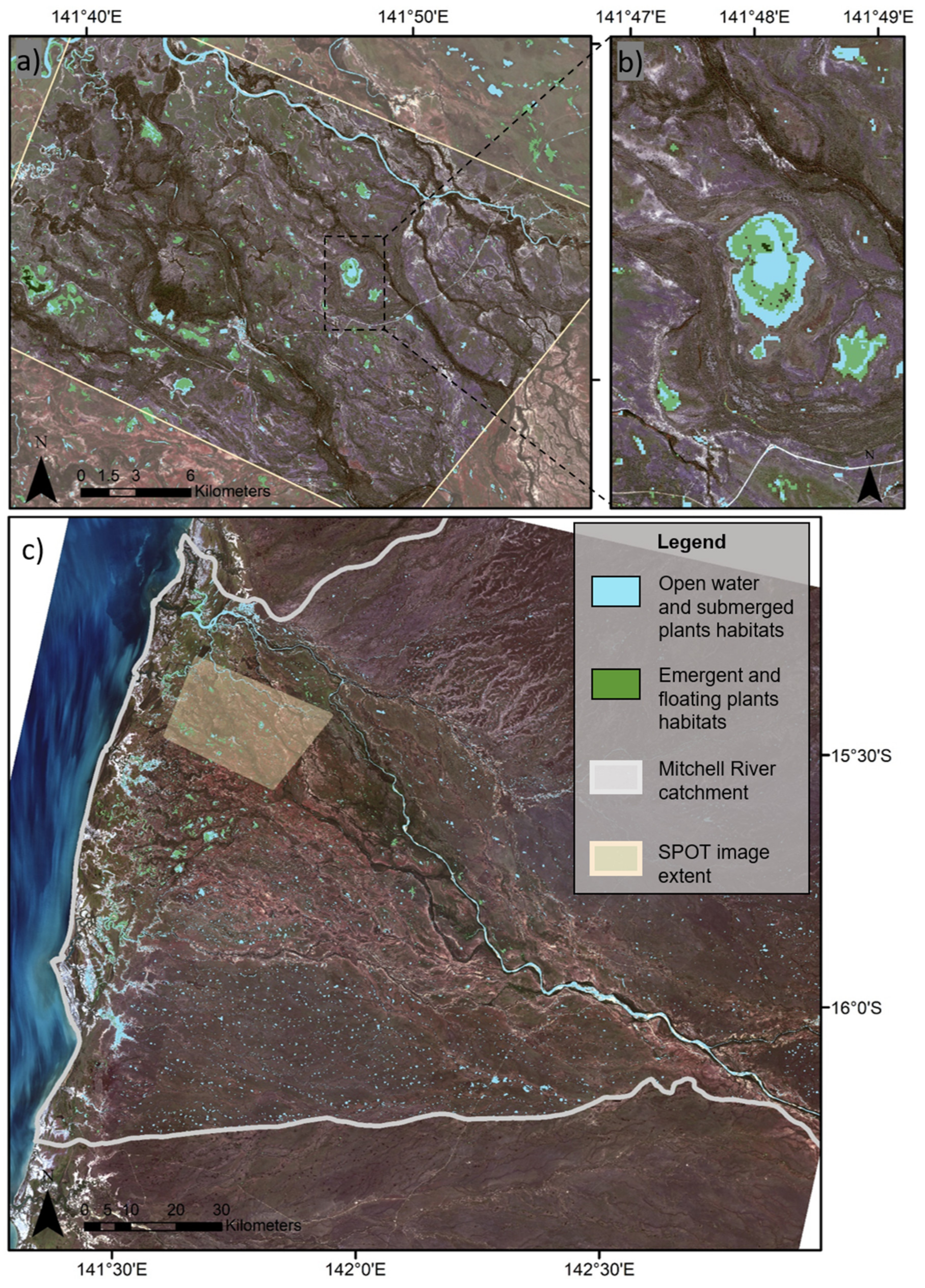
3.1. Statistical Modelling of Habitat Type

The most important predictors of habitat type, based on variable importance, were the Landsat 8 MNDWI and OSAVI (Figure 4). The classification tree modelling showed that the MNDWI was the most important predictor of the inundated areas, with pixels below the threshold value of –0.4 being classed as water. Within inundated areas, the OSAVI was the most important predictor of the open water and open water with submerged plants and emergent and floating plants classes with pixels above the threshold of 0.4 being classed as the latter. For sand distribution, a NDSI threshold of 0.34 was used to mask the sand pixels. The accuracy of the classification tree modelling of habitat type resulted in an overall accuracy of 93%. While 189 observations of open water were correctly classified, 18 observations were misclassified as emergent and floating plant habitats. Additionally, 80 observations were correctly classified as emergent and floating plant habitats, while three observations were misclassified as open water habitats.
The predictions of the classification tree indicated that the freshwater flooded extent of the Mitchell River floodplain was dominated by open water and submerged plant habitats in April 2017 (Figure 5). Approximately, 79% (47.8 km2) of the flooded pixels were classified in this way with only 21% (12.9 km2) as emergent and floating aquatic plant habitats. The results from the model indicated that the floating and emergent plant habitats were predominantly predicted to occur around the edges of the wetlands. Areas of open water habitat were usually located on the middle of large water bodies and on the rivers and channels across the floodplain.

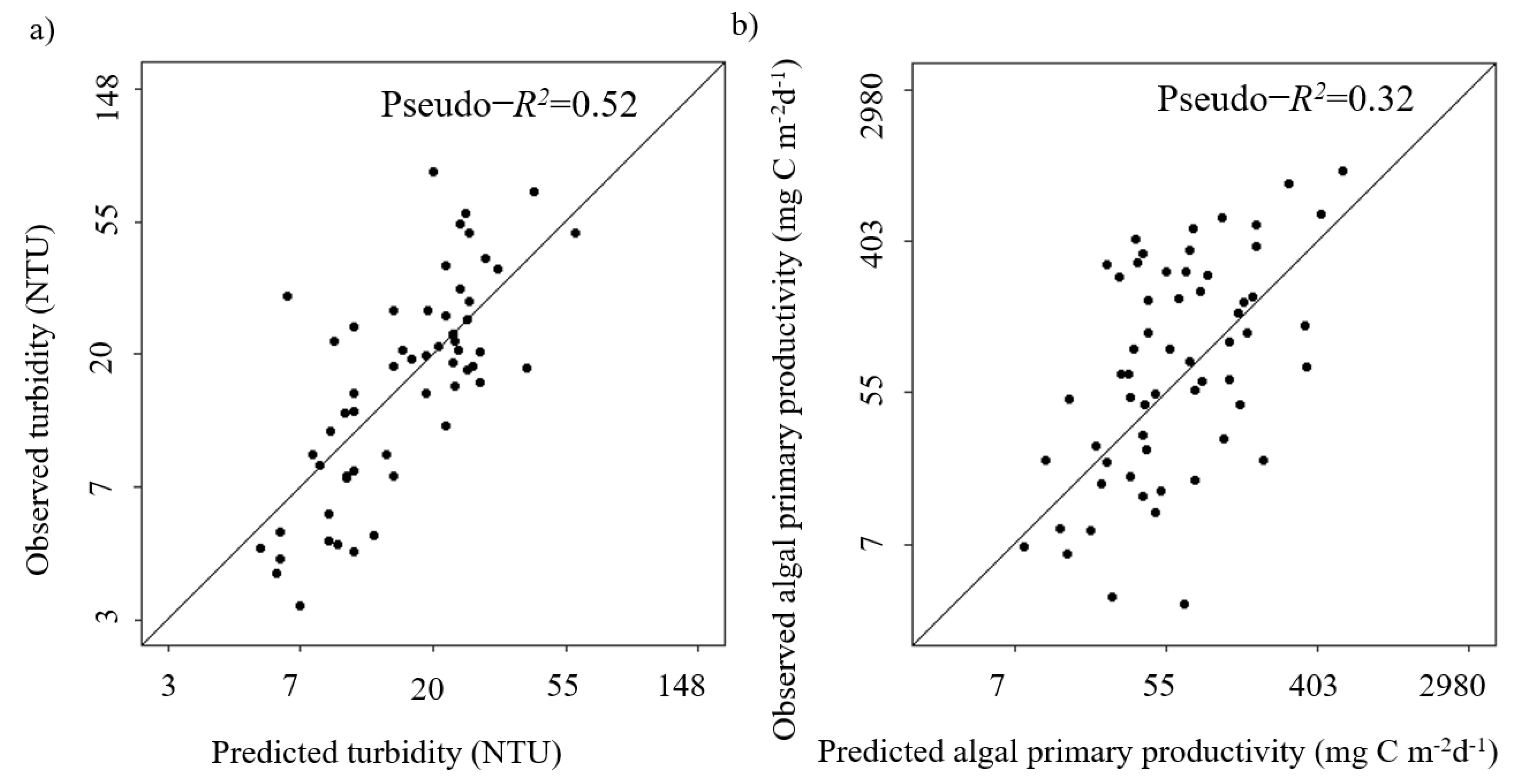
3.2. Statistical Modelling of Turbidity

The best fitting statistical model to estimate turbidity, identified by the AIC, explained 52% of the variation of turbidity (pseudo-R2 = 0.52, Figure 6a). The model included habitat type and the Landsat OLI green (band 3) and red bands (band 4) as predictors (Table 3). The green band was negatively related to turbidity while the red band was positively related to turbidity. Predicted turbidity across the Mitchell River floodplain under the model ranged from 1.4 to 117.4 NTU (Figure 7). Approximately 75% of the pixels had predicted turbidity under 16.2 NTU (Figure A2a) and the mean predicted turbidity was 15.6 ± 10.9 SD NTU. Spatially, turbidity tended to be higher in the river channels and in the coastal area of the Mitchell River floodplain. However, within the same river system or wetland there is a smaller difference between the predicted turbidity values, for example, on racecourse swamp, turbidity ranged between 1.4 and 22 NTU (Figure 7b).

3.3. Statistical Modelling of Algal Primary Productivity

The statistical model of algal primary productivity, that included habitat type and turbidity as predictors, explained 32% of variation (pseudo-R2 = 0.32, Table 3, Figure 6b). The average predictive performance of this model was 47% and the RMSLE was 1.33, indicating reasonable predictive performance. The spatial predictions of rates of primary production ranged from 3.2 to 859.2 (Figure 8) with a mean of 150.9 ± 95.47 mg C m−2 d−1 (SD). Across the majority of the floodplain, algal productivity was predicted between 100 and 200 mg C m−2 d−1 (Figure A2b). The higher predictions of algal productivity were located on secondary river channels, small wetlands, and littoral areas (Figure 8). The difference between the lower and upper 95% predictive intervals were larger for those pixels with greater algal productivity prediction, usually located in turbid areas in the littoral areas of the floodplain (Figure A3). The rates of algal primary production within the Mitchell River floodplain were equivalent to a total daily production of 85.02 ± 0.07 ton C d−1 (SD) (with a prediction interval from 84.9 to 85.6 ton C). From the total production, only about 6% of this was located in the main rivers of the floodplains, while the remaining algal production was located on the wetlands across the floodplain.

4. Discussion

The approach developed in this study provides a methodology to predict rates of algal primary production by integrating field work, statistical modelling, and remote sensing techniques. This study showed that most of the algal productivity in the Mitchell River floodplain, accounting for both periphyton and phytoplankton, occurred in the wetlands across the whole floodplain. Predicting algal productivity across an entire floodplain has the potential to improve wetland conservation by identifying key productive habitats that are important sources of food for aquatic consumers. Accounting for ecological processes can represent an important tool to improve floodplain management and conservation [66]. Floodplain ecosystems have been experiencing changing environmental and flow conditions, and such approach can be used to predict broader ecosystem responses [27]. By providing end users with knowledge and spatial data for the identification of those critical habitats, this approach can be feed directly into the management of the Mitchell River floodplain. Additionally, this approach could be adapted to other floodplains worldwide that are under pressure from development, or from climate change, to prevent habitat loss and hence preserve system biodiversity.
Despite the increased use of remote sensing for monitoring water quality and ecological processes, its use for these purposes in inland waters is still limited compared to coastal waters, because of the higher complexity of inland waters [67]. Although, some more recent studies have used remote sensing techniques to estimate algal abundance on lakes and floodplains [6,11,20], algal productivity studies are still largely limited to field work-based approaches [8,10,32]. The statistical model previously developed for the Mitchell River floodplain to capture the spatial nature of algal primary productivity provided the means to build on field approaches, and combine the use of satellite remote sensing [9]. While remote sensing itself cannot directly estimate rates of algal production, the prediction of habitat type (as type of aquatic plant cover or absence) and turbidity is feasible [25,26,55], and these serve as useful proxies to predict algal productivity.
Due to the importance of aquatic macrophytes for determining algal growth [8,9], it was first necessary to capture the spatial variation of habitat type across the floodplain. We found that MNDWI and the OSAVI indices were the best predictors of water and the presence of rooted aquatic plants. Both indices have been previously adopted for floodplains studies; for example, MNDWI was used to predict the presence of water [68,69] and OSAVI was used to predict vegetation biomass [69]. Identifying the best set of predictors and the thresholds for classification allows for the prediction of key productive habitats across larger areas, which can be used as inputs for further analysis, e.g., for periphyton abundance studies [20] and for turbidity [25].
We also assessed the spatial variation in turbidity, as turbidity was found to be an important predictor of algal productivity on the Mitchell River floodplain [9]. Turbidity was assessed by retrieving habitat type variation, and the green and red spectral reflectance characteristics from the Landsat 8 image, as those were identified as important predictors of turbidity. Habitat type and these spectral bands were also found to be important predictors of turbidity in other regions [25,70,71,72]. The inclusion of habitat type as a predictor takes into account the spectral interference of aquatic plants on the prediction of turbidity [25]. The red and the green spectral bands were used as predictors of turbidity because the increase of scattering, with increasing concentrations of suspended particles in water, results in greater reflectance on the red band than on the green band [71,72]. Other studies have developed models to predict turbidity across different region around the world, including the Mitchell River, using remotely sensed data, with higher accuracy [25,70]. This previous study in Mitchell River hade considerably larger range of observed turbidity values, due to sampling across different seasons, which likely helped to improve model accuracy. Our model, despite lower accuracy was developed and calibrated to the study region and time that field work took place making it an appropriate choice for this study. Improvements in future modelling of turbidity could come from longer sampling periods and potentially integrating our model results as prior information in a Bayesian model [73]. The identification of the predictors of habitat type and turbidity facilitated prediction of their spatial variation using satellite remote sensing, and subsequently the prediction of algal primary productivity across the Mitchell River floodplain.
The approach developed in this study predicted total daily algal production across the floodplain and the results showed high production on the Mitchell River floodplain relative to the river channels. Our findings suggested that the majority of the total algal carbon produced on the Mitchell River floodplain was located outside of the main river channels, in floodplain wetlands. In shallow wetlands, like the ones found on the Mitchell River floodplain, the relatively high levels of light penetration favor phytoplankton productivity and dense macrophyte cover promotes periphyton attachment and growth [22,74]. Additionally, algal primary productivity is likely to be even higher on peak inundation days or in wetter years where more floodplain wetlands get inundated for longer [25]. This suggests that maintaining connectivity between floodplain wetlands and the river channel is likely to be important in supporting instream secondary production.
Other studies had also found that relatively isolated wetlands can support high productivity [40] and play an important role for metapopulations [75]. Our results emphasize the likely importance of floodplain wetlands in sustaining ecosystem functioning of the Mitchell River. While those wetlands may just be inundated for a short period, past studies have shown the importance of floodplain food sources in supporting aquatic food webs [2]. The important subsidies that floodplain wetlands provide for aquatic consumers in rivers relies on floodplain connectivity, either facilitating mobile consumers to move out onto the inundated floodplain, or as floodwaters recede, prey are washed back into the river [76]. By identifying the spatial variation of algal productivity, this approach enables natural resource managers to understand where the key sources of carbon may be located and to identify habitats where maintaining inundation and connectivity is likely to be important for ecosystem function [77,78].
The algal primary productivity model (including epiphyton and phytoplankton productivity) developed in this study presented relatively lower accuracy compared to well-established models developed to measure phytoplankton biomass in open water habitats using remotely sensed data [19,79]. The modelling of an ecological process such as algal primary productivity, compared to a more static metric such as biomass, is complicated by the large number of variables influencing this process, such as nutrients, water movement, and light [7,80]. Additionally, algal productivity is a highly dynamic process with hydro-meteorological conditions influencing those rates [81,82]. The map of the predictive intervals shows areas where model uncertainty is greatest, and this information can be used to guide sampling in future research. Future studies can build upon our approach and models by including more sampling locations to support remotely sensed information, within the constraints of the remote sampling location. A final step that would help improve model accuracy would be the development of remote sensing tools that can distinguish between open water and submerged macrophytes across different water conditions to accommodate the different rates of primary productivity that can occur in those habitats [83].

5. Conclusions

This study provides a transferrable methodology to map algal productivity at large spatial scales and identify ‘hotspots’ (areas of high algal productivity), by using spectral indices and bands from Landsat 8 remotely sensed images. We have applied this methodology to map the spatial variation in algal productivity across the Mitchell River floodplain and identified that most of the production occurs on the floodplain wetlands. However, these areas can only provide high quality food resources to consumers from the riverine environment, such as fish, if the fish can access the wetlands and return to the river. Landscape connectivity, facilitated by floodplain inundation, facilitates organisms’ access to these hotspots. Planned agricultural development in the Mitchell River basin and the likely impacts of water resource development on the hydrological regime may cause floodplain wetlands habitats that are important sources of algal production to be inundated for shorter durations or become inaccessible to higher order consumers [84,85]. Combining our approach with landscape connectivity analyses may help identify the impact of changing surface water dynamics on algal production inputs to river–floodplain ecosystems. We showed that the use of remote sensing to predict an ecological process such as algal productivity is feasible. As much of the source data for such analyses can also be derived from satellites, these approaches can be applied beyond the Mitchell River. Further developments in remote sensing technology and ongoing data collection will only help to improve approaches such as ours, thereby providing greater utility for floodplain management and conservation.

Author Contributions

Conceptualization, B.M., B.S.-K. and S.E.B.; methodology, B.M.; formal analysis, B.M.; data curation, B.M. and T.J.M.; writing—original draft preparation, B.M.; writing—review and editing, B.M., B.S.-K., T.J.M. and S.E.B.; supervision, B.S.-K., T.J.M., S.E.B. All authors have read and agreed to the published version of the manuscript.

Funding

This research is supported with funding from the Australian Government’s National Environmental Science Program. The APC was funded by the Australian Government’s National Environmental Science Program.

Data Availability Statement

Landsat 8 data are available from: https://earthexplorer.usgs.gov/ (accessed on 24 September 2018).

Acknowledgments

The authors thank the Kowanyama Aboriginal Land and Natural Resource Management Office for the assistance with field collections. We acknowledge the traditional owners of the country from which the samples were collected in the Mitchell River catchment. We also thank Graeme Curwen and Cristopher Ndehedehe for their support with the spatial analysis. This project was carried out as part of the lead author’s PhD research at the Australian Rivers Institute, Griffith University, with financial support of Griffith University (postgraduate funding) and the Australian Government’s National Environmental Science program (NESP) (including top-up scholarship).

Conflicts of Interest

The authors declare no conflict of interest.

Appendix A

Figure A1. The hyetograph and hydrograph at the Dunbar gauging station from 1 October 2017 to 30 September 2018. The rainfall and discharge data at the Dunbar gauging station from those dates were obtained from the Queensland Water Monitoring Information Portal (https://water-monitoring.information.qld.gov.au/ accessed on 4 June 2021).
Remotesensing 13 01710 g0a1
Figure A2. Histogram of the predicted values of (a) turbidity and (b) algal primary productivity across the Landsat Image.
Remotesensing 13 01710 g0a2
Figure A3. Spatial distribution of the difference between the upper and the lower prediction interval of each algal primary productivity prediction across (a) a small portion of the floodplain and (b) the Mitchell River floodplain extent.
Remotesensing 13 01710 g0a3

References

  1. Bunn, S.; Ward, D.; Crook, D.A.; Jardine, T.; Adame, F.; Pettit, N.; Douglas, M.M.; Valdez, D.; Kyne, P.M. Tropical Floodplain Food Webs—Connectivity and Hotspots—Final Report; Charles Darwin University: Darwin, Australia, 2015. [Google Scholar]
  2. Jardine, T.D.; Pusey, B.J.; Hamilton, S.K.; Pettit, N.E.; Davies, P.M.; Douglas, M.M.; Sinnamon, V.; Halliday, I.A.; Bunn, S.E. Fish mediate high food web connectivity in the lower reaches of a tropical floodplain river. Oecologia 2012, 168, 829–838. [Google Scholar] [CrossRef]
  3. Jardine, T.D.; Hunt, R.; Faggotter, S.; Valdez, D.; Burford, M.; Bunn, S. Carbon from periphyton supports fish biomass in waterholes of a wet-dry tropical river. River Res. Appl. 2013, 29, 560–573. [Google Scholar] [CrossRef] [Green Version]
  4. Saigo, M.; Zilli, F.L.; Marchese, M.R.; Demonte, D. Trophic level, food chain length and omnivory in the Paraná River: A food web model approach in a floodplain river system. Ecol. Res. 2015, 30, 843–852. [Google Scholar] [CrossRef]
  5. Brett, M.T.; Bunn, S.E.; Chandra, S.; Galloway, A.W.E.; Guo, F.; Kainz, M.J.; Kankaala, P.; Lau, D.C.P.; Moulton, T.P.; Power, M.E.; et al. How important are terrestrial organic carbon inputs for secondary production in freshwater ecosystems? Freshw. Biol. 2017, 62, 833–853. [Google Scholar] [CrossRef]
  6. Kuhn, C.D.; Bogard, M.; Johnston, S.E.; John, A.; Vermote, E.F.; Spencer, R.; Dornblaser, M.; Wickland, K.P.; Striegl, R.G.; Butman, D. Satellite and airborne remote sensing of gross primary productivity in boreal Alaskan lakes. Environ. Res. Lett. 2020, 15, 105001. [Google Scholar] [CrossRef]
  7. Vadeboncoeur, Y.; Devlin, S.; McIntyre, P.; Vander Zanden, J. Is there light after depth? Distribution of periphyton chlorophyll and productivity in lake littoral zones. Freshw. Sci. 2014, 33, 524–536. [Google Scholar] [CrossRef] [Green Version]
  8. Adame, M.F.; Pettit, N.E.; Valdez, D.; Ward, D.; Burford, M.A.; Bunn, S.E. The contribution of epiphyton to the primary production of tropical floodplain wetlands. Biotropica 2017, 49, 461–471. [Google Scholar] [CrossRef] [Green Version]
  9. Molinari, B.; Stewart-Koster, B.; Adame, M.F.; Campbell, M.D.; McGregor, G.; Schulz, C.; Malthus, T.J.; Bunn, S. Relationships between algal primary productivity and environmental variables in tropical floodplain wetlands. Inland Waters 2021, 1–11. [Google Scholar] [CrossRef]
  10. Jia, J.; Gao, Y.; Zhou, F.; Shi, K.; Johnes, P.J.; Dungait, J.A.J.; Ma, M.; Lu, Y. Identifying the main drivers of change of phytoplankton community structure and gross primary productivity in a river-lake system. J. Hydrol. 2020, 583, 124633. [Google Scholar] [CrossRef]
  11. Vis, C.; Hudon, C.; Carignan, R.; Gagnon, P. Spatial Analysis of Production by Macrophytes, Phytoplankton and Epiphyton in a Large River System under Different Water-Level Conditions. Ecosystems 2007, 10, 293–310. [Google Scholar] [CrossRef]
  12. Garcia, E.A.; Townsend, S.A.; Douglas, M.M. Context dependency of top-down and bottom-up effects in a Northern Australian tropical river. Freshw. Sci. 2015, 34, 679–690. [Google Scholar] [CrossRef]
  13. Polis, G.A. Why Are Parts of the World Green? Multiple Factors Control Productivity and the Distribution of Biomass. Oikos 1999, 86, 3–15. [Google Scholar] [CrossRef]
  14. Thompson, R.M.; Townsend, C.R. Energy Availability, Spatial Heterogeneity and Ecosystem Size Predict Food-Web Structure in Streams. Oikos 2005, 108, 137–148. [Google Scholar] [CrossRef]
  15. Palmer, S.C.J.; Kutser, T.; Hunter, P.D. Remote sensing of inland waters: Challenges, progress and future directions. Remote Sens. Environ. 2015, 157, 1–8. [Google Scholar] [CrossRef] [Green Version]
  16. Zolfaghari, K.; Duguay, C.R. Estimation of water quality parameters in Lake Erie from MERIS using Linear mixed effect models. Remote Sens. 2016, 8, 473. [Google Scholar] [CrossRef] [Green Version]
  17. Tyler, A.N.; Svab, E.; Preston, T.; Présing, M.; Kovács, W.A. Remote sensing of the water quality of shallow lakes: A mixture modelling approach to quantifying phytoplankton in water characterized by high-suspended sediment. Int. J. Remote Sens. 2006, 27, 1521–1537. [Google Scholar] [CrossRef]
  18. Watanabe, F.S.Y.; Alcantara, E.; Rodrigues, T.W.P.; Imai, N.N.; Barbosa, C.C.F.; Rotta, L.H.D. Estimation of Chlorophyll-a Concentration and the Trophic State of the Barra Bonita Hydroelectric Reservoir Using OLI/Landsat-8 Images. Int. J. Environ. Res. Public Health 2015, 12, 10391–10417. [Google Scholar] [CrossRef]
  19. Rotta, L.; Alcântara, E.; Park, E.; Bernardo, N.; Watanabe, F. A single semi-analytical algorithm to retrieve chlorophyll-a concentration in oligo-to-hypereutrophic waters of a tropical reservoir cascade. Ecol. Indic. 2021, 120, 106913. [Google Scholar] [CrossRef]
  20. Ward, D.P.; Pettit, N.E.; Adame, M.; Douglas, M.M.; Setterfield, S.A.; Bunn, S.E. Seasonal spatial dynamics of floodplain macrophyte and periphyton abundance in the Alligator Rivers region (Kakadu) of northern Australia: Kakadu Seasonal Dynamics of Macrophytes and Epiphytic Algae. Ecohydrology 2016, 9, 1675–1686. [Google Scholar] [CrossRef]
  21. Pettit, N.E.; Bayliss, P.; Davies, P.M.; Hamilton, S.K.; Warfe, D.M.; Bunn, S.E.; Douglas, M.M. Seasonal contrasts in carbon resources and ecological processes on a tropical floodplain. Freshw. Biol. 2011, 56, 1047–1064. [Google Scholar] [CrossRef] [Green Version]
  22. Pettit, N.E.; Ward, D.P.; Adame, M.F.; Valdez, D.; Bunn, S.E. Influence of aquatic plant architecture on epiphyte biomass on a tropical river floodplain. Aquat. Bot. 2016, 129, 35–43. [Google Scholar] [CrossRef] [Green Version]
  23. Costa, M. Estimate of net primary productivity of aquatic vegetation of the Amazon floodplain using Radarsat and JERS-1. Int. J. Remote Sens. 2005, 26, 4527–4536. [Google Scholar] [CrossRef]
  24. Güttler, F.N.; Niculescu, S.; Gohin, F. Turbidity retrieval and monitoring of Danube Delta waters using multi-sensor optical remote sensing data: An integrated view from the delta plain lakes to the western–northwestern Black Sea coastal zone. Remote Sens. Environ. 2013, 132, 86–101. [Google Scholar] [CrossRef] [Green Version]
  25. Ward, D.; Hamilton, S.; Jardine, T.; Pettit, N.; Tews, K.; Olley, J.; Bunn, S. Assessing the seasonal dynamics of inundation, turbidity, and aquatic vegetation in the Australian wet–dry tropics using optical remote sensing. Ecohydrology 2013, 6, 312–323. [Google Scholar] [CrossRef] [Green Version]
  26. Malthus, T.J. Chapter 9—Bio-optical Modeling and Remote Sensing of Aquatic Macrophytes. In Bio-Optical Modeling and Remote Sensing of Inland Waters; Mishra, D.R., Ogashawara, I., Gitelson, A.A., Eds.; Elsevier: Amsterdam, The Netherlands, 2017; pp. 263–308. [Google Scholar]
  27. Reid, A.J.; Carlson, A.K.; Creed, I.F.; Eliason, E.J.; Gell, P.A.; Johnson, P.T.J.; Kidd, K.A.; MacCormack, T.J.; Olden, J.D.; Ormerod, S.J.; et al. Emerging threats and persistent conservation challenges for freshwater biodiversity. Biol. Rev. 2019, 94, 849–873. [Google Scholar] [CrossRef] [PubMed] [Green Version]
  28. Karim, F.; Peña-Arancibia, J.; Ticehurst, C.; Marvanek, S.; Gallant, J.; Hughes, J.; Dutta, D.; Vaze, J.; Petheram, C.; Seo, L.; et al. Floodplain Inundation Mapping and Modelling for the Fitzroy, Darwin and Mitchell Catchments; A Technical Report to the Australian Government from the CSIRO Northern Australia Water Resource Assessment, Part of the National Water Infrastructure Development Fund: Water Resource Assessments; CSIRO: Canberra, Australia, 2018.
  29. Stoeckl, N.; Stanley, O. Key Industries in Australia’s Tropical Savanna. Australas. J. Reg. Stud. 2007, 13, 255–286. [Google Scholar]
  30. Australian Government. Our North, Our Future: White Paper on Developing Northern Australia; Department of the Prime Minister and Cabinet: Canberra, Australia, 2015.
  31. Ndehedehe, C.E.; Onojeghuo, A.O.; Stewart-Koster, B.; Bunn, S.E.; Ferreira, V.G. Upstream flows drive the productivity of floodplain ecosystems in tropical Queensland. Ecol. Indic. 2021, 125, 107546. [Google Scholar] [CrossRef]
  32. Burford, M.A.; Webster, I.T.; Revill, A.T.; Kenyon, R.A.; Whittle, M.; Curwen, G. Controls on phytoplankton productivity in a wet–dry tropical estuary. Estuar. Coast. Shelf Sci. 2012, 113, 141–151. [Google Scholar] [CrossRef] [Green Version]
  33. Flood, N.; Danaher, T.; Gill, T.; Gillingham, S. An operational scheme for deriving standardised surface reflectance from landsat TM/ETM+ and SPOT HRG imagery for eastern Australia. Remote Sens. 2013, 5, 83–109. [Google Scholar] [CrossRef] [Green Version]
  34. Pohl, C.; Van Genderen, J.L. Review article Multisensor image fusion in remote sensing: Concepts, methods and applications. Int. J. Remote Sens. 2010, 19, 823–854. [Google Scholar] [CrossRef] [Green Version]
  35. Breiman, L. Classification and Regression Trees; Wadsworth International Group: Belmont, CA, USA, 1984. [Google Scholar]
  36. Therneau, T.; Atkinson, B. Package ‘rpart’: Recursive Partitioning and Regression Trees. R Package Version 4.1-15. 2019. Available online: https://CRAN.R-project.org/package=rpart (accessed on 6 June 2020).
  37. R Development Core Team. R: A Language and Environment for Statistical Computing; R Foundation for Statistical Computing: Vienna, Austria, 2019. [Google Scholar]
  38. Davranche, A.; Lefebvre, G.; Poulin, B. Wetland monitoring using classification trees and SPOT-5 seasonal time series. Remote Sens. Environ. 2010, 114, 552–562. [Google Scholar] [CrossRef] [Green Version]
  39. Zhao, D.; Jiang, H.; Yang, T.; Cai, Y.; Xu, D.; An, S. Remote sensing of aquatic vegetation distribution in Taihu Lake using an improved classification tree with modified thresholds. J. Environ. Manag. 2012, 95, 98–107. [Google Scholar] [CrossRef]
  40. Ndehedehe, C.E.; Burford, M.A.; Stewart-Koster, B.; Bunn, S.E. Satellite-derived changes in floodplain productivity and freshwater habitats in northern Australia (1991–2019). Ecol. Indic. 2020, 114, 106320. [Google Scholar] [CrossRef]
  41. Feyisa, G.L.; Meilby, H.; Fensholt, R.; Proud, S.R. Automated Water Extraction Index: A new technique for surface water mapping using Landsat imagery. Remote Sens. Environ. 2014, 140, 23–35. [Google Scholar] [CrossRef]
  42. Gao, B.-C. NDWI—A normalized difference water index for remote sensing of vegetation liquid water from space. Remote Sens. Environ. 1996, 58, 257–266. [Google Scholar] [CrossRef]
  43. McFeeters, S.K. The use of the Normalized Difference Water Index (NDWI) in the delineation of open water features. Int. J. Remote Sens. 1996, 17, 1425–1432. [Google Scholar] [CrossRef]
  44. Xu, H. Modification of normalised difference water index (NDWI) to enhance open water features in remotely sensed imagery. Int. J. Remote Sens. 2006, 27, 3025–3033. [Google Scholar] [CrossRef]
  45. Sims, N.; Anstee, J.; Barron, O.; Botha, E.; Lehmann, E.; Li, L.; McVicar, T.; Paget, M.; Ticehurst, C.; Van Niel, T.; et al. Earth Observation Remote Sensing; A Technical Report to the Australian Government from the CSIRO Northern Australia Water Resource Assessment, Part of the National Water Infrastructure Development Fund: Water Resource Assessments; CSIRO: Canberra, Australia, 2016.
  46. Steven, M.D. The Sensitivity of the OSAVI Vegetation Index to Observational Parameters. Remote Sens. Environ. 1998, 63, 49–60. [Google Scholar] [CrossRef]
  47. Xue, J.; Su, B. Significant Remote Sensing Vegetation Indices: A Review of Developments and Applications. J. Sens. 2017, 2017, 1–17. [Google Scholar] [CrossRef] [Green Version]
  48. Fern, R.R.; Foxley, E.A.; Bruno, A.; Morrison, M.L. Suitability of NDVI and OSAVI as estimators of green biomass and coverage in a semi-arid rangeland. Ecol. Indic. 2018, 94, 16–21. [Google Scholar] [CrossRef]
  49. Pan, X.; Zhu, X.; Yang, Y.; Cao, C.; Zhang, X.; Shan, L. Applicability of Downscaling Land Surface Temperature by Using Normalized Difference Sand Index. Sci. Rep. 2018, 8, 9530. [Google Scholar] [CrossRef] [PubMed] [Green Version]
  50. Lymburner, L.; Botha, E.; Hestir, E.; Anstee, J.; Sagar, S.; Dekker, A.; Malthus, T. Landsat 8: Providing continuity and increased precision for measuring multi-decadal time series of total suspended matter. Remote Sens. Environ. 2016, 185, 108–118. [Google Scholar] [CrossRef]
  51. Lillesand, T.M.; Kiefer, R.W.; Chipman, J.W. Remote Sensing and Image Interpretation, 5th ed.; John Wiley: New York, NY, USA, 2004. [Google Scholar]
  52. Burman, P. A Comparative Study of Ordinary Cross-Validation, v-Fold Cross-Validation and the Repeated Learning-Testing Methods. Biometrika 1989, 76, 503–514. [Google Scholar] [CrossRef] [Green Version]
  53. James, G.; Witten, D.; Hastie, T.; Tibshirani, R. An Introduction to Statistical Learning: With Applications in R; Springer: New York, NY, USA, 2013. [Google Scholar]
  54. Petheram, C.; Watson, I.; Bruce, C.; Chilcott, C. Water Resource Assessment for the Mitchell Catchment; A Report to the Australian Government from the CSIRO Northern Australia Water Resource Assessment, Part of the National Water Infrastructure Development Fund: Water Resource Assessments; CSIRO: Canberra, Australia, 2018.
  55. Bustamante, J.; Pacios, F.; Díaz-Delgado, R.; Aragonés, D. Predictive models of turbidity and water depth in the Doñana marshes using Landsat TM and ETM+ images. J. Environ. Manag. 2009, 90, 2219–2225. [Google Scholar] [CrossRef]
  56. Chen, Z.; Hu, C.; Muller-Karger, F. Monitoring turbidity in Tampa Bay using MODIS/Aqua 250-m imagery. Remote Sens. Environ. 2007, 109, 207–220. [Google Scholar] [CrossRef]
  57. Xing, L.W.; Niu, Z.G. Mapping and analyzing China’s wetlands using MODIS time series data. Wetl. Ecol. Manag. 2019, 27, 693–710. [Google Scholar] [CrossRef]
  58. Bates, D.; Mächler, M.; Bolker, B.; Walker, S. Fitting Linear Mixed-Effects Models Using lme4. J. Stat. Softw. 2015, 67, 1–48. [Google Scholar] [CrossRef]
  59. Hurvich, C.M.; Tsai, C.-L. Regression and Time Series Model Selection in Small Samples. Biometrika 1989, 76, 297. [Google Scholar] [CrossRef]
  60. Nakagawa, S.; Schielzeth, H.; O’Hara, R.B. A general and simple method for obtaining R2 from generalized linear mixed-effects models. Methods Ecol. Evol. 2013, 4, 133–142. [Google Scholar] [CrossRef]
  61. Halekoh, U.; Højsgaard, S. A Kenward-Roger Approximation and Parametric Bootstrap Methods for Tests in Linear Mixed Models—The R Package pbkrtest. J. Stat. Softw. 2014, 59, 32. [Google Scholar] [CrossRef] [Green Version]
  62. Jachner, S.; Boogaart, G.; Petzoldt, T. Statistical Methods for the Qualitative Assessment of Dynamic Models with Time Delay (R Package qual V). J. Stat. Softw. 2007, 22, 1–30. [Google Scholar] [CrossRef] [Green Version]
  63. Knowles, J.E.; Frederick, C. merTools: Tools for Analyzing Mixed Effect Regression Models. 2020. Available online: https://CRAN.R-project.org/package=merTools (accessed on 25 September 2020).
  64. Dei Rossi, J.A. Prediction Intervals for Summed Totals; Rand Corporation: Santa Monica, CA, USA, 1968. [Google Scholar]
  65. Lane, D.M.; David, S.; Mikki, H.; Rudy, G.; Dan, O.; Zimmer, H. Introduction to Statistics; Rice University: Houston, TX, USA; University of Houston Clear Lake: Houston, TX, USA; Tufts University: Medford, MA, USA, 2013. [Google Scholar]
  66. Reis, V.; Hermoso, V.; Hamilton, S.K.; Bunn, S.E.; Linke, S. Conservation planning for river-wetland mosaics: A flexible spatial approach to integrate floodplain and upstream catchment connectivity. Biol. Conserv. 2019, 236, 356–365. [Google Scholar] [CrossRef]
  67. Malthus, T.J.; Hestir, E.L.; Dekker, A.G.; Brando, V.E. The Case for a Global Inland Water Quality Product. In Proceedings of the 2012 IEEE International Geoscience and remote sensing Symposium, Munich, Germany, 22–27 July 2012; pp. 5234–5237. [Google Scholar]
  68. Huang, C.; Wu, J.; Chen, Y.; Yu, J. Detecting Floodplain Inundation Frequency Using MODIS Time-Series Imagery. In Proceedings of the 2012 First International Conference on Agro- Geoinformatics (Agro-Geoinformatics), Shanghai, China, 2–4 August 2012; pp. 1–6. [Google Scholar]
  69. Ndehedehe, C.E.; Stewart-Koster, B.; Burford, M.A.; Bunn, S.E. Predicting hot spots of aquatic plant biomass in a large floodplain river catchment in the Australian wet-dry tropics. Ecol. Indic. 2020, 117, 106616. [Google Scholar] [CrossRef]
  70. Quang, N.H.; Sasaki, J.; Higa, H.; Huan, N.H. Spatiotemporal variation of turbidity based on landsat 8 OLI in Cam Ranh Bay and Thuy Trieu Lagoon, Vietnam. Water 2017, 9, 570. [Google Scholar] [CrossRef] [Green Version]
  71. Bid, S.; Siddique, G. Identification of seasonal variation of water turbidity using NDTI method in Panchet Hill Dam, India. Modeling Earth Syst. Environ. 2019, 5, 1179–1200. [Google Scholar] [CrossRef]
  72. Pham, Q.; Ha, N.; Pahlevan, N.; Oanh, L.; Nguyen, T.; Nguyen, N. Using Landsat-8 Images for Quantifying Suspended Sediment Concentration in Red River (Northern Vietnam). Remote Sens. 2018, 10, 1841. [Google Scholar] [CrossRef] [Green Version]
  73. McCarthy, M.A.; Masters, P. Profiting from prior information in Bayesian analyses of ecological data. J. Appl. Ecol. 2005, 42, 1012–1019. [Google Scholar] [CrossRef]
  74. Hinojosa-Garro, D.; Mason, C.F.; Underwood, G.J.C. Influence of macrophyte spatial architecture on periphyton and macroinvertebrate community structure in shallow water bodies under contrasting land management. Fundam. Appl. Limnol. 2010, 177, 19–37. [Google Scholar] [CrossRef]
  75. Leibowitz, S.G. Isolated wetlands and their functions: An ecological perspective. Wetlands 2003, 23, 517–531. [Google Scholar] [CrossRef]
  76. Sparks, R.E. Need for ecosystem management of large rivers and their floodplains—These phenomenally productive ecosystems produce fish and wildlife and preserve species. Bioscience 1995, 45, 168–182. [Google Scholar] [CrossRef]
  77. Pettit, N.E.; Naiman, R.J.; Warfe, D.M.; Jardine, T.D.; Douglas, M.M.; Bunn, S.E.; Davies, P.M. Productivity and Connectivity in Tropical Riverscapes of Northern Australia: Ecological Insights for Management. Ecosystems 2017, 20, 492–514. [Google Scholar] [CrossRef] [Green Version]
  78. Furst, D.J.; Aldridge, K.T.; Shiel, R.J.; Ganf, G.G.; Mills, S.; Brookes, J.D. Floodplain connectivity facilitates significant export of zooplankton to the main River Murray channel during a flood event. Inland Waters 2014, 4, 413–424. [Google Scholar] [CrossRef]
  79. Duan, H.; Ma, R.; Xu, J.; Zhang, Y.; Zhang, B. Comparison of different semi-empirical algorithms to estimate chlorophyll-a concentration in inland lake water. Environ. Monit. Assess. 2010, 170, 231–244. [Google Scholar] [CrossRef] [PubMed]
  80. Gosselain, V.R.; Hudon, C.; Cattaneo, A.; Gagnon, P.; Planas, D.; Rochefort, D. Physical variables driving epiphytic algal biomass in a dense macrophyte bed of the St. Lawrence River (Quebec, Canada). Hydrobiologia 2005, 534, 11–22. [Google Scholar] [CrossRef]
  81. Burford, M.A.; Valdez, D.; Curwen, G.; Faggotter, S.J.; Ward, D.P.; O’Brien, K.R. Inundation of saline supratidal mudflats provides an important source of carbon and nutrients in an aquatic system. Mar. Ecol. Prog. Ser. 2016, 545, 21–33. [Google Scholar] [CrossRef] [Green Version]
  82. Saravia, L.A.; Momo, F.; Boffi Lissin, L.D. Modelling periphyton dynamics in running water. Ecol. Model. 1998, 114, 35–47. [Google Scholar] [CrossRef]
  83. Rowan, G.S.L.; Kalacska, M. A Review of Remote Sensing of Submerged Aquatic Vegetation for Non-Specialists. Remote Sens. 2021, 13, 623. [Google Scholar] [CrossRef]
  84. Tockner, K.; Pusch, M.; Borchardt, D.; Lorang, M.S. Multiple stressors in coupled river-floodplain ecosystems. Freshw. Biol. 2010, 55, 135–151. [Google Scholar] [CrossRef]
  85. Mukherjee, K.; Pal, S. Hydrological and landscape dynamics of floodplain wetlands of the Diara region, Eastern India. Ecol. Indic. 2021, 121, 106961. [Google Scholar] [CrossRef]
Figure 1. Study region showing thetopographic distribution (elevation in meters) and major river channels in the Mitchell River catchment. The dash box refers to the floodplain extent. The inset shows the location of the Mitchell River catchment (dark grey) within Australia. The gauging station for observed flow and rainfall data is also indicated.
Remotesensing 13 01710 g001
Figure 2. Schematic representation of the methodological framework used in this study.
Remotesensing 13 01710 g002
Figure 3. The Mitchell River catchment, location of sampling sites, and extent of remotely sensed images: (a) the Mitchell River catchment in grey and the dashed box refers to the extent of the Landsat 8, (b) the Landsat 8 image with the extent of the SPOT image in shade beige and the Mitchell River catchment boarders in grey; (c) the SPOT 7 Image in the beige contour, the background corresponds to the Landsat 8 image. The colored points show the location of the wetlands where field data was collected (orange for lacustrine, green for palustrine, and yellow for riverine wetlands).
Remotesensing 13 01710 g003
Figure 4. Results of the classification tree analysis for floodplain cover states showing the best performing model (MNDWI + OSAVI + NDSI) to predict the cover states for the Mitchell River floodplain.
Remotesensing 13 01710 g004
Figure 5. Classified wetland habitat distribution across (a) the SPOT image extent; (b) a smaller portion of the floodplain consisting of Racecourse Swamp; and (c) the Landsat 8 image extent. Grey lines represent the Mitchell catchment boundary, and the light beige shaded area indicates the SPOT image extent. Blue pixels are the open water and open water with submerged habitats and green pixels are the emergent and floating plants habitats.
Remotesensing 13 01710 g005
Figure 6. Observed and predicted values of (a) turbidity and (b) algal primary productivity. All axes were log-transformed.
Remotesensing 13 01710 g006
Figure 7. Spatial variation of turbidity (NTU) across (a) the SPOT image extent; (b) a small portion of the floodplain consisting of Racecourse wetland; and (c) the Landsat 8 image extent. Grey lines represent the Mitchell catchment boundary, and the light beige shaded area indicates the SPOT image extent.
Remotesensing 13 01710 g007
Figure 8. Spatial variation of predicted algal primary productivity (mg C m−2 d−1) across (a) the Spot image extent; (b) a small fraction of the floodplain consisting of Racecourse Swamp; and (c) the Landsat 8 image extent. Grey lines represent the Mitchell catchment boundary, and the light beige indicates the SPOT image extent.
Remotesensing 13 01710 g008
Table 1. The spectral, spatial characteristics of Landsat 8 OLI and SPOT 7 images used in this study.
Landsat 8 OLI SPOT 7
Date of Acquisition25 April 201825 April 2018
Spatial resolution30 m6 m
Spectral bands:Wavelengths (nm)
Coastal Aerosol (CA)435–451NA
Blue452–512450–520
Green533–590530–590
Red636–673625–695
Near Infrared (NIR)851–879760–890
Shortwave NIR 1 (SWIR 1)1566–1651NA
Shortwave NIR 2 (SWIR 2)2107–2294NA
Table 2. Formulae for the spectral indices and TSM using Landsat 8 OLI bands tested to differentiate land, open water, and plant habitats in this study.
Spectral IndicesFormulaReference
Automated water extraction index (AWEI)4(Green − SWIR) − 0.25(0.25 × NIR + 2.75 × SWIR)[41]
Normalized difference water index (NDWI)(Green − NIR)/(Green + NIR)[43]
Modified normalized difference water index (MNDWI)(Green − SWIR)/(Green + SWIR)[44]
Optimized soil adjusted vegetation index (OSAVI)(NIR − Red)/(NIR + Red + 0.16)[46]
Normalized difference vegetation index (NDVI)(NIR − Red)/(NIR + Red)[42]
Normalized difference sand index (NDSI)(Red − Coastal aerosol)/(Red − Coastal aerosol)[49]
Total suspended matter (TSM)3957 × (TSM_index) ^ 1.6436;
TSM_index = (green_band/10,000 + red_band/10,000)/2
[50]
Table 3. Coefficients of the Turbidity and Algal Primary Productivity (PP) models and standard errors (Std. Error). The reference level for Habitat Type is open water and open water with submerged plants. The response variables were log-transformed.
Turbidity Model PP Model
Parameter
Estimate
Std. Errorp ValueParameter
Estimate
Std. Errorp Value
Intercept 2.8984860.413495<0.0013.12560.7505<0.001
Habitat Type Floating + Emergent0.4349200.1760970.02−1.76090.4182<0.001
Green Band −0.0047590.0020770.04--
Red Band 0.0041760.0017450.04--
Log (turbidity-NTU) -- 0.74350.2605 0.02
Publisher’s Note: MDPI stays neutral with regard to jurisdictional claims in published maps and institutional affiliations.

