Article

Data-Driven Approaches for Tornado Damage Estimation with Unpiloted Aerial Systems

1
School of Earth and Space Exploration, Arizona State University, Tempe, AZ 85281, USA
2
Cooperative Institute for Mesoscale Meteorological Studies, The University of Oklahoma, Norman, OK 73019, USA
3
School of Environmental Sciences, University of Liverpool, Liverpool L69 3BX, UK
4
School of Geographical Sciences and Urban Planning, Arizona State University, Tempe, AZ 85281, USA
*
Author to whom correspondence should be addressed.
Remote Sens. 2021, 13(9), 1669; https://doi.org/10.3390/rs13091669
Submission received: 26 March 2021 / Revised: 19 April 2021 / Accepted: 20 April 2021 / Published: 25 April 2021

Abstract

:
Tornado damage estimation is important for providing insights into tornado studies and assisting rapid disaster response. However, it is challenging to precisely estimate tornado damage because of the large volumes of perishable data. This study presents data-driven approaches to tornado damage estimation using imagery collected from Unpiloted Aerial Systems (UASs) following the 26 June 2018 Eureka Kansas tornado. High-resolution orthomosaics were generated from Structure from Motion (SfM). We applied deep neural networks (DNNs) on the orthomosaics to estimate tornado damage and assessed their performance in four scenarios: (1) object detection with binary categories, (2) object detection with multiple categories, (3) image classification with binary categories, and (4) image classification with multiple categories. Additionally, two types of tornado damage heatmaps were generated. By directly stitching the resulting image tiles from the DNN inference, we produced the first type of tornado damage heatmaps where damage estimates are accurately georeferenced. We also presented a Gaussian process (GP) regression model to build the second type of tornado damage heatmap (a spatially continuous tornado damage heatmap) by merging the first type of object detection and image classification heatmaps. The GP regression results were assessed with ground-truth annotations and National Weather Service (NWS) ground surveys. This detailed information can help NWS Weather Forecast Offices and emergency managers with their damage assessments and better inform disaster response and recovery.

1. Introduction

Tornadoes are considered one of the most destructive forces of nature because of their intense winds (high wind speeds) and resulting damage [1]. There are approximately 1000 tornadoes annually in the US, killing 60 people and producing 982 million US dollars in economic damages [2,3]. Because direct measurements of tornadic winds are rare and difficult to obtain, damage assessments are used to infer wind speeds using the Enhanced Fujita (EF) Scale [4]. In addition to rating tornado intensity, damage assessments provide valuable information for emergency management operations and disaster recovery. Obtaining timely and accurate damage information improves disaster recovery and facilitates better decision-making with regard to resource allocation and planning [5].
Conventional damage assessments (ground-based and satellite surveys) are restricted by available resources, accessibility, and technological limitations. Ground surveys, conducted by the local National Weather Service Weather Forecast Offices (NWS WFOs) following severe weather events, provide the most detailed information but are both time- and resource-intensive [6]. Additionally, these surveys can still be subjective despite damage indicators and engineering guidelines [4]. Satellite imagery has been used in hurricane damage assessment [7]. Because of the need for coverage conducted immediately after the event, satellite imagery cannot often be directly applied to tornado damage estimation. Satellite imagery also cannot provide enough resolution for detailed, object-level damage estimation.
UAS damage surveys can provide valuable information needed for detailed tornado damage assessments. In assessing the damage of the Canton Texas tornado, Wagner et al. [8] visualized the tornado damage by manually thresholding multispectral orthomosaics generated by Structure from Motion (SfM) based on Unpiloted Aerial System (UAS) imagery. Even though UAS can give rapid access to high-resolution and georeferenced imagery almost immediately after weather events, one problem is maintaining manual analysis of such voluminous data. Direct human oversight of the analysis considerably slows the total damage estimation process. Automation of the tornado damage estimation using UAS imagery could produce many benefits. By automating high-resolution damage estimation, emergency managers could make rapid and precise disaster responses. Such automation could also assist insurance companies in estimating economic losses.
Data-driven approaches can help automate tornado damage estimation. For example, fully connected neural networks were used to predict tornado-induced property damage using publicly available data [9], which includes high-level information such as where and when a tornado occurred, tornado path length and width, and how much property damage it caused. Le et al. [10] employed a fully connected neural network as a surrogate model for the performance assessment of a vertical structure subjected to non-stationary, tornadic wind loads. However, without using detailed information such as image features, those studies only examined tornado damage at a macroscale level. Finer detailed information such as trees, roofs, and debris is needed to provide more precise damage information.
Convolutional neural networks (CNNs) have achieved unprecedented results in image processing such as image classification [11], segmentation [12], and object detection [13], leading to broad applications in structural feature detection [14,15] and condition assessment [16,17]. In satellite-based assessments, CNNs have been used to classify hurricane-damaged roofs [18] and to estimate tree failure due to high winds [19,20]. Recently, unsupervised and semisupervised learning approaches leveraged a large number of unlabeled data to extract structural features in satellite images [21,22]. With UAS imagery, Cheng et al. [23] used Mask R-CNN [13], a more advanced neural network based on CNN, to detect and segment tornado-damaged buildings. Their study, however, did not produce accurate geolocations of damaged buildings because Mask R-CNN was directly applied to UAS imagery, which lacks pixel-level locational information. A comprehensive review of UAS-based structural damage mapping has been reviewed by Kerle et al. [24]. Other studies used CNNs to classify building damage with multi-resolution images from unpiloted aerial vehicles, piloted aerial vehicles, and satellites [25,26], but these studies have not investigated object-level feature detection.
From 2D images to 3D point clouds, DNNs have also been applied to estimate tornado damage using point clouds generated by SfM. 3D fully convolutional networks (FCNs) were used to segment 3D voxels rasterized from post-wind point clouds [27,28]. 3D voxel segmentation requires values for every voxel in 3D grids, including empty spaces, which were labeled as neutral in their work [27,28]. This additional information could have affected the accuracy of their results by adding to the imbalanced training dataset problem [29]. Therefore, although the neutral (empty spaces) and terrain had reached high precision and recall, their studies only noted the highest precision of 31% and the highest recall of 33% on the tornado damage related features such as debris, undamaged structures, and damaged structures. While their studies provide a foundation for tornado damage estimation, tornado damage heatmaps, which provide geolocation information of damage estimates, are still needed for a more comprehensive damage assessment.
The goal of this work is to present data-driven approaches for tornado damage estimation and to provide spatially explicit tornado damage heatmaps. UAS surveys were deployed to collect aerial images after an EF3 tornado hit the city of Eureka, Kansas, in June 2018. We estimated tornado damage by applying DNNs on tiled images that were split from orthomosaics generated by SfM. Four scenarios were investigated: (1) object detection with binary categories, (2) object detection with multiple categories, (3) image classification with binary categories, and (4) image classification with multiple categories. Additionally, two types of tornado damage heatmaps were generated. The first tornado damage heatmap was produced directly stitching the resulting image tiles from the DNN inference. The second type of tornado damage heatmap was generated via Gaussian process (GP) regression that merged the first type of object detection and image classification heatmaps. Both types of heatmaps provided accurate geolocations of tornado damage estimates, necessary for improving emergency response and disaster recovery. The presented data-driven approaches in this study could also assist NWS WFOs in refining tornado damage estimation and insurance companies with improving economic loss estimation.

2. Materials and Methods

2.1. Study Area

On 26 June 2018, an EF3 tornado hit the city of Eureka, Kansas injuring eight people and causing 13.69 million USD in damage losses [30]. Although the tornado had a reported damage path length of 13.03 km (8.1 miles) and width of 0.45 km (0.28 miles), the majority of damage losses occurred along a one-mile section of the path located in downtown Eureka (Figure 1). This study focuses on structural damage in this one-mile section.

2.2. Data Collection

2.2.1. Uas Survey Data

Four subsequent UAS surveys were conducted to obtain post-tornado event imagery. A DJI Inspire 2, equipped with a Zenmuse x5s 20 megapixel camera, was flown at 91 m (300 feet) above ground level. RGB imagery was collected using near nadir angle and 75% front and side overlap to achieve 3D reconstruction through SfM [31]. Approximately 3996 images were collected from 27 June 2018 under relatively cloud-free skies and sufficient illumination conditions. Ground control points (GCPs) were measured using a Trimble Geo7x handheld GNSS system with an accuracy of ±0.04 m. Thirty GCPs were collected using easily identifiable photo features such as manholes, valve covers, and intersections of sidewalks and driveways. Horizontal positions were referenced to the 1984 World Geodetic Datum State Plane 1502 Kansas South, and vertical positions were referenced to NAD88.

2.2.2. Ground Survey Data

Ground survey data were obtained from the NWS WFO Wichita, Kansas via the Damage Assessment Toolkit [32] (Figure 1). Following a tornado event, NWS meteorologists assigned EF-scale ratings in their ground surveys based on damage indicators and wind engineer standards [1,4]. These data points with EF-scale ratings were provided in the World Geodetic System 1984 coordinate system.

2.3. Structure from Motion

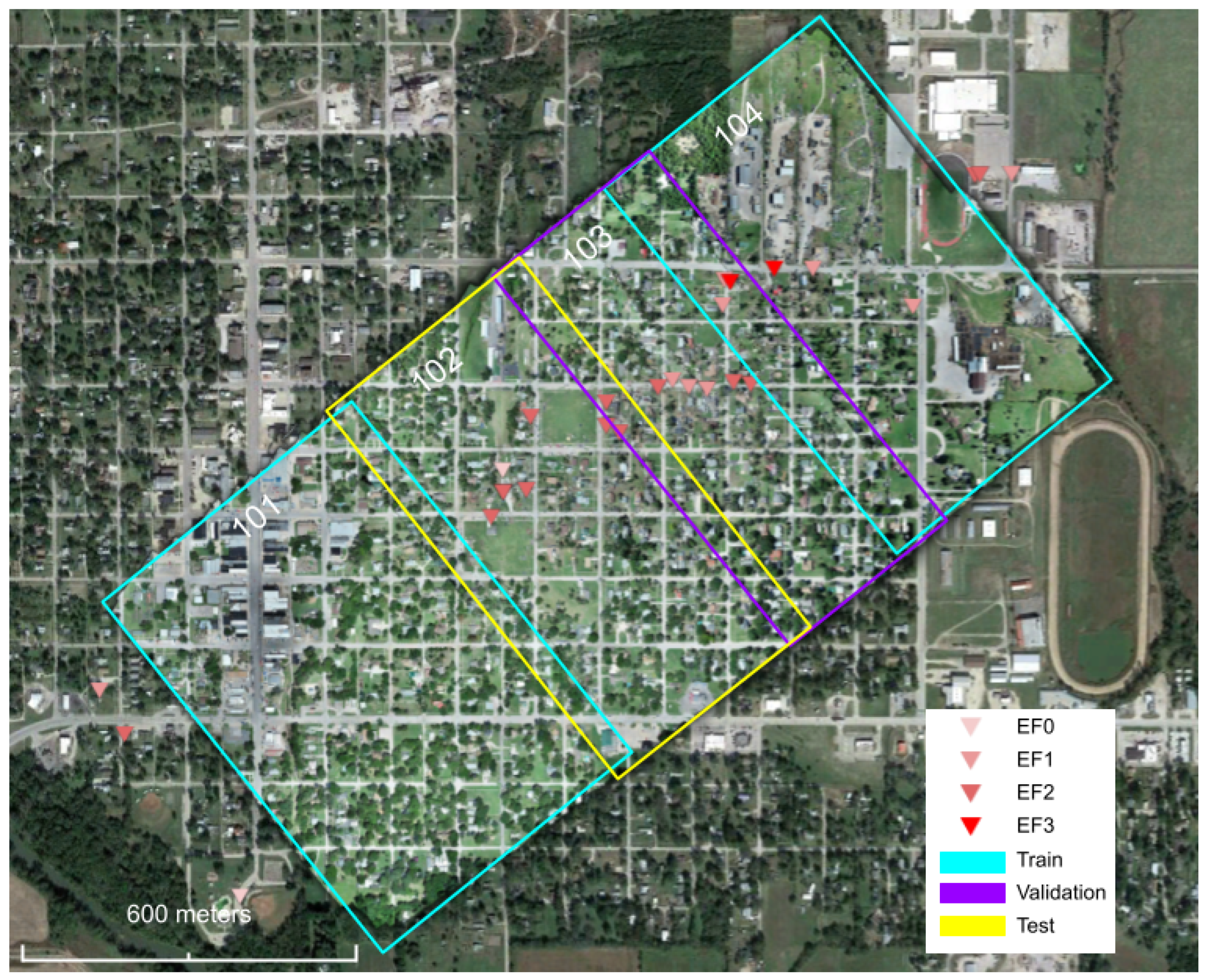
UAS imagery was processed using Agisoft Photoscan Professional [33] to generate post-event 3D model products and orthomosaics (~2 cm/pixel resolution). GCPs were incorporated into SfM to rectify global distortions [34]. Post-event orthomosaics, from four UAS surveys, were used for neural network training, validating, and testing, as shown in Figure 2. Despite geological overlaps between the sections, because the orthomosaics were generated from four subsequent UAS surveys, the SfM orthomosaics on the overlap areas are different regarding lighting conditions, SfM artifacts, and data preparation. Examples of the orthomosaics on the overlap areas are presented in Appendix A.

2.4. Deep Learning

This study deployed deep learning (DL) models to estimate tornado damage at specific object and general image levels. A DNN was trained to detect residential buildings among five classes, including “no damage”, and then “EF0” to “EF3”, which was the highest EF scale in the tornado path. In addition to object detection, we separately classified image tiles with three damage categories of “no damage”, “minor damage”, and “major damage”. By directly stitching the resulting image tiles from the DNN inference, we generated the first type of tornado damage heatmap, where damage estimates were accurately georeferenced. The workflow diagram of deep learning is shown in Figure 3a.

2.4.1. Data Preparation

Following the data preparation process in the UAS-SfM-DL pipeline [35], orthomosaics were split into 2000 × 2000 pixel image tiles such that the average residential building coverage (the ratio of a residential building area to a tile area) was about 10.3%, considering the average house size in Kansas of 165.6 square meters. The size of 2000 × 2000 pixels, however, still required large neural network models (parameter number) and GPU global memory. These tiles were bilinearly reshaped to 1000 × 1000 pixel size (~4 cm/pixel resolution) to accommodate GPU global memory and avoid losing details of damage features.
Labelbox [36] was used to annotate image tiles for object detection and image classification. For object detection, we used polygons to bound all buildings with five categories ranging from “no damage” to “EF3” on the EF scale. For image classification, image tiles were annotated based on three damage categories, i.e., “no damage”, “minor damage”, and “major damage” (Table 1). “Major damage” was based on structural damage, not strewn debris or tree damage. For example, an image tile with “roof structure failure” was annotated as “major damage”, whereas an image tile with only “major broken trunk” was annotated as “minor damage”. Most of the image tiles were annotated except a few with SfM artifacts such as distortions and blanks. For image classification, the image tile numbers for the four sections (101~104) are 423, 375, 336, and 400, respectively, resulting in the training: validation: test dataset ratio of 0.54: 0.22: 0.24. Some image tiles without any buildings were omitted for object detection. The annotation data sizes are summarized in Figure 4. We invested 22 work hours to annotate residential buildings and 8 work hours to annotate image tile classes.
Because the data sizes for different categories were imbalanced for object detection and image classification (Figure 4), we investigated this problem with two methods. First, we converted the original categories into a binary categorization of “no damage” versus “damage” for both object detection and image classification annotations. The new “no damage” category still included the original “no damage” category members; the new “damage” category included everything except the original “no damage” category members. Therefore, the re-categorized datasets are more balanced. To evaluate the recategorization method, we conducted object detection and image classification for both the original multi-class datasets and new binary-class datasets. The second method augmented the training data with different augmentation weights such that the augmented datasets were balanced. The data augmentation process adopted the conventional image augmentation methods such as random combinations of up-down flipping, left-right flipping, rotation, zooming in, and zooming out. The zooming in or out was implemented by bilinear interpolation with scaling factors randomly selected between 0.8 and 1.2, such that the resultant ground sampling distances ranged from 3.3 to 5 cm/pixel.

2.4.2. Neural Network Training

Mask R-CNN [13] was selected as the deep neural network architecture for object detection. Pyramid Feature Network (PFN) [37] was exploited as the backbone of the Mask R-CNN. PFN’s multi-scale, pyramidal-hierarchical anchor generation mechanism can facilitate object detection for buildings with various pixel sizes in image tiles. The various pixel sizes of buildings are majorly caused by orthomosaic splitting. For example, some residential buildings split by image tile boundaries have small pixel sizes because of their partial presentation; other buildings not cut off may have larger pixel sizes.
For image classification, we investigated several the state-of-the-art DNN architectures such as ResNet-152 [11], Wide ResNet-101 [38], ResNeXt-101 [39], DenseNet-161, and DenseNet-201 [40]. All the neural networks were implemented using Torchvision [41], a package consisting of popular datasets, model architectures, and common image transformations for computer vision.
This study adopted transfer learning because of its advances demonstrated in the previous work [35]. The weights of the Mask R-CNN were initialized with a model well-trained from COCO 2017 [42], except that the last layer was modified to accommodate the class numbers in this study. We initialized the image classification network weights with models well-trained from ImageNet [43] and also reshaped the last layer accordingly. The last layers of the neural networks were decided by the class numbers, as the number of multiple classes or binary classes for object detection or image classification. With the assistance of transfer learning, we trained the Mask R-CNN on an Nvidia RTX 2080 Ti for 8 h on average and image classification networks for 4 h on average.

2.4.3. Neural Network Evaluation

The neural networks were trained with the training datasets (101 and 104 image tiles), and the validation datasets (103 image tiles) were used to inspect the neural network performance every training epoch. The neural networks with the best performance on the validation datasets were assessed on the test datasets (102 image tiles).
For object detection, intersection over union (IoU) between bounding boxes from prediction and ground truth was used to determine true positives and false positives:
IoU = A p A t A p A t ,
where A p is the area of the prediction bounding box, and A t is the area of the ground-truth bounding box. If IoU is greater than an IoU threshold, the prediction bounding box is considered as a true-positive detection, otherwise as a false-positive detection. When a ground-truth bounding box does not have overlap with any prediction bounding boxes, this case is considered as a false-negative detection.
We used mean-Average-Precision (mAP) and mean-Average-recall (mAR) to measure object detection performance:
m A P ( I o U = α ) = 1 S c = 1 S T P c ( I o U = α ) T P c ( I o U = α ) + F P c ( I o U = α ) m A R ( I o U = α ) = 1 S c = 1 S T P c ( I o U = α ) T P c + F N c ( I o U = α ) ,
where α { 0.5 , 0.55 , 0.6 , , 0.95 } is the IoU threshold, S is the number of categories, T P c is the number of true positives for the c-th category, F P c is the number of false positives, and F N c is the number of false negatives. When only one IoU threshold (e.g., 0.5) was considered, m A P ( I o U = 0.5 ) denoted the mAP of the object detection with the IoU threshold of 0.5. This denotation was similarly applied to mAR. The object detection performance was also examined with a list of IoU thresholds. For example, I o U = [0.5:0.95] denoted a list of IoU thresholds, { 0.5 , 0.55 , 0.6 , , 0.95 } . As such, we averaged the mAPs and mARs of the list IoU thresholds,
m A P ( I o U = [ 0.5 : 0.95 ] ) = 1 10 [ m A P ( I o U = 0.5 ) + m A P ( I o U = 0.55 ) + . . . + m A P ( I o U = 0.95 ) ] m A R ( I o U = [ 0.5 : 0.95 ] ) = 1 10 [ m A R ( I o U = 0.5 ) + m A R ( I o U = 0.55 ) + . . . + m A R ( I o U = 0.95 ) ] .

2.4.4. Post-Processing

The objective of the neural network post-processing is to build tornado damage heatmaps from the neural network inference results. We conducted object detection and image classification inference on image tiles from sections 102 and 103, producing heatmap tiles. The heatmap tiles have the same size (1000 × 1000 pixels) as the input image tiles. For object detection, the heatmap tiles contain residential building masks detected and classified from Mask R-CNN; for image classification, all the pixels in a heatmap tile are noted with one prediction category. The heatmap tiles were resized back to 2000 × 2000 pixels using bilinear interpolation. The resized heatmap tiles were then stitched together to compose large heatmaps with the same size as the original orthomosaics such that the large heatmaps have consistent georeferences with the original orthomosaics.
As shown in Figure 2, there are overlaps between adjacent survey sections (101~104). The object detection or image classification may have different damage estimates on the overlap areas. To merge the object detection or image classification heatmaps from two adjacent sections, we kept the higher damage estimates on the overlap areas. Object detection inference examples and heatmaps are shown in Figures 5 and 6; image classification inference examples and heatmaps are shown in Figures 7 and 8.

2.5. Gaussian Process Regression

While the heatmaps from object detection and image classification have advantages of straightforward implementation by using existing software packages, these two damage representations have not been collectively exploited; however, they could provide compensatory information for tornado damage estimation when incorporated jointly. Object detection focuses on specific features such as residential buildings, whereas the image classification discerns features from all over the image tiles. These two heatmaps should have a high correlation on damage estimates. For example, image tiles with detected damaged buildings should reflect a similar trend of damage estimates from image classification. Therefore, a joint representation from object detection and image classification could contain more complete and accurate damage information. We used Gaussian process (GP) regression [44], also known as Kriging in geostatistics, to incorporate the inference results from the object detection and image classification, building a spatially continuous tornado damage heatmap. The workflow diagram of the GP regression is presented in Figure 3b. Definition nuances between DL and GP terminologies by convention are clarified in Appendix B. “Labels” mentioned in this article refer to the neural network inference results and ground-truth annotations.

2.5.1. GP Regression Scheme

A scheme of the GP regression is presented as follows. We denote a GP training dataset as D = { X , Y } = { < x 1 , y 1 > , < x 2 , y 2 > , , < x N , y N > } , where X = [ x 1 , x 2 , , x N ] T are sample locations and Y = [ y 1 , y 2 , , y 3 ] T are corresponding tornado damage labels from object detection or image classification. The input spatial location x and output tornado damage y can be modeled by an abstract function:
y = f ( x ) + e ( x ) ,
where f ( x ) is a trend function, and e ( x ) is a residual noise component. The residual noises are drawn from independent, identically distributed Gaussian distribution with zero mean and σ n 2 variance. The GP regression assumes that the joint probability p ( y 1 , y 2 , , y N ) is Gaussian, with mean μ ( X ) and covariance Σ ( X ) given Σ i j = κ ( x i , x j ) . The mean μ ( X ) is usually set as 0 , and κ ( · ) is a positive definite kernel function:
κ ( x i , x j ) = σ f 2 e 1 2 l 2 | | x i x j | | 2 + σ n 2 δ i j ,
where σ n 2 , l, and σ f are GP hyperparameters that can be learned from training, and δ i j is a Kronecker delta. δ i j is 1 iff i = j otherwise 0. Once the GP regression model has been trained using the GP training dataset D, given a GP test dataset X , we can predict corresponding tornado damage labels Y from the GP regression model [44]:
p ( Y | X , X , Y ) = N ( Y | μ , Σ ) μ = K T [ K + σ n 2 I ] 1 Y Σ = K K T [ K + σ n 2 I ] 1 K ,
where K i j = κ ( x i , x j ) , K i j = κ ( x i , x j ) , and K i j = κ ( x i , x j ) . Pixel coordinates were used for X and X . The values for Y were determined by object detection and image classification labels and their neighborhood adjustment. Section 2.5.3 introduces how X, X , and Y were determined in detail. We used the mean of GP inference μ to present prediction tornado damage. That is, Y = μ .
To evaluate this method, we independently conducted the GP regression on the data from neural network inference results and ground-truth annotations. The GP regression results from the annotations were considered as ground truth and then compared with the GP regression results from neural network inference. Since the trained neural networks have lower inference performance on the DL validation and test data (102 and 103) than DL training data (101 and 104), which is shown in Section 3, we focused on the worse scenario and thus conducted and evaluated the GP regression using labels from 102 and 103.

2.5.2. Model Efficiency Techniques

Directly applying data points from object detection and image classification heatmaps to the conventional GP regression will be problematic. The data points only from the object detection (ranging from “no damage” to “EF3” on Figure 6c) comprise over 134,000,000 pixels. The computation complexity in time of the conventional GP regression is O ( N 3 ) , where N is the number of data points in the GP training dataset; e.g., N > 134,000,000 if only using detection data. The time complexity is predominantly caused by inverting the kernel matrix [ K + σ n 2 I ] 1 . The GP training and inference processes are very inefficient because of the cubic time complexity and large data points.
We used two techniques to improve the model efficiency. Gpytorch [45] was applied for the GP regression implementation. Gpytorch first reduces the asymptotic time complexity of GP from O ( N 3 ) to O ( N 2 ) via Blackbox Matrix-Matrix multiplication and further accelerates the computing with GPU hardware. Additionally, we downsampled the merged object detection and image classification heatmaps to 200 × 200 pixel rasters using the maximum values of the nearest neighbors, such that the GP training and inference data point sizes were also reduced. The combination of these acceleration techniques enabled us to efficiently conduct GP training and inference using an Nvidia 1060 with 6 GB global memory.

2.5.3. Sampling Strategy

In this subsection, we present the sampling strategy used to obtain the GP training and test datasets. To generate a more precise tornado damage heatmap, we exploited multi-class scenarios for both object detection and image classification. From the annotations and neural network inference results, the GP regression used eight heatmaps: four heatmaps from object detection and image classification inference on 102 and 103, and the other four from their corresponding ground-truth annotations. The heatmap pairs of 102 and 103 were merged (Section 2.4.4) to obtain four merged heatmaps, which are the merged multi-class object detection inference heatmap H d (Figure 6c), the merged multi-class image classification inference heatmap H c (Figure 8c), and their corresponding ground-truth heatmaps, H d (Figure 6d) and H c (Figure 8d). These four merged heatmaps were further downsampled to 200 × 200 pixel rasters (Section 2.5.2): R d , R c , R d , and R c . For the remainder of this Section 2.5.3, we use the inference rasters ( R d and R c ) to illustrate the sampling strategy. The same process was applied to the ground-truth rasters ( R d and R c ).
The objective of the sampling strategy is to determine values for the GP training dataset D = { X , Y } and test dataset X , such that we can estimate tornado damage Y using the GP regression (Section 2.5.1). It is straightforward to determine X , which is a set of pixel coordinates of all the pixels on a 200 × 200 raster. Determining the GP training dataset D = { X , Y } is tricky because the GP training dataset needs to incorporate data from object detection and image classification.
We let X consist of the pixel coordinates of all valid pixels on R d and part of valid pixels randomly sampled from R c . Valid pixels denote those pixels where there are object detection or image classification labels as opposed to no data. All valid pixels on R d were included because object detection labels are already sparse (19% of raster pixels), and the set of their pixel coordinates is denoted as X d . We uniformly sampled 30% of the valid pixels on R c , and denote the set of their pixel coordinates as X c . The input of the GP training dataset was the union of the two pixel-coordinate sets, X = X d X c . There are two reasons for not including all valid pixels on R c . First, including all valid pixels on R c will add a computational burden. Second, we expect a smooth underlying fitting function from the GP regression, but including all the valid pixels could result in a bumpy fitting function.
After having obtained the input of the training dataset X, we determine the corresponding output dataset Y. There are three categories in image classification labels and five in object detection labels. To incorporate them, we need to have consistent category numbers wherever a data point is from. A neighborhood adjustment method was presented for this purpose. We first initialized object detection and image classification rasters ( R d and R c ) with values for each label. The conversion from labels to values is shown in the round brackets in Table 2. Then, the associated object detection or image classification values in R d or R c could be represented as functions, r d = R d ( x ) or r c = R c ( x ) , where r d { 0 , 1 , 2 , 3 , 4 , 5 } and r c { 0 , 1 , 2 , 3 } . The remaining processes were as follows: given a pair of pixel coordinates x X ( X = X d X c ), we first separately obtained object detection damage estimate y d and image classification damage estimate y c and then combined y d and y c to obtain y.
The following formula was used to obtain y d Y d :
y d ( x d ) = T d ( R d ( x d ) , R c ( x d ) ) ,
where x d X d is a pair of pixel coordinates from object detection rasters, and T d ( · ) is a lookup table (Table 2) to determine y d . The first argument of T d ( · ) is the object detection value at x d , and the second argument is the image classification value at the same pixel coordinates. The rationale of the lookup table T d ( · ) is to adjust the object detection value R d ( x d ) based on its corresponding image classification value R c ( x d ) at the same pixel coordinates.
To obtain y c Y c , we cannot do the same thing as when we got y d . The reason is that, given valid pixel coordinates from image classification rasters x c X c , there might be no data in the object detection rasters at the same pixel coordinates, because the valid pixels on object detection rasters are sparser than on image classification rasters. The sparseness difference is illustrated by comparing Figures 6 and 8. Instead of using a detection value at exactly the same pixel coordinates x c , we found the nearest n valid data points (in Euclidean distance) in the object detection rasters and then used the average of the object detection values from the nearest n data points as the object detection value for another lookup table (Table 3). The processes are described by the following formulas:
r d = 1 n i = 1 n R d ( N i ( x c ) ) y c ( x c ) = T c ( R c ( x c ) , r d ) ,
where x c X c is a pair of pixel coordinates from image classification rasters, N i is the pixel coordinates of the i-th nearest valid data point in the object detection rasters around x c , r d [ 0 , 5 ] is the average object detection value of the nearest n valid data points ( n = 5 ), and T c ( · ) is a lookup table (Table 3) to determine y c . The first argument of T c ( · ) is the image classification value at x c , and the second argument is the average detection value r d . The lookup table T c ( · ) is designed to obtain y c from the image classification value R c ( x c ) with the adjustment based on the average object detection value r d . We implemented the nearest neighbor search by a K-D tree [46]. K-D tree algorithm is efficient for the n nearest search complexity of O ( n l o g ( M ) ) , where M is the total valid pixel number in a detection raster. Lastly, we obtained y by overlaying y d and y c :
Y = { m a x ( y d ( x ) , y c ( x ) ) | x X } .

2.5.4. Monte Carlo Sampling

Because a GP training dataset X includes the coordinates of the valid pixels uniformly sampled from image classification rasters, the GP inference results μ vary slightly with different samples. To address this problem, we consider the GP training dataset X as a random variable. μ is a function of the random variable X, because μ is a function of Y (Equation (5)) and Y is a function of X (Equation (8)). The objective is then framed to find the expectation of the GP inference results:
μ ¯ = p ( X ) μ ( X ) d X ,
where p ( X ) is a probability density function of X. This integral, however, is intractable to solve. Instead, we used Monte Carlo sampling to approximate the expectation:
μ ^ = 1 T i = 1 T μ ( X i ) ,
where X i is composed of the pixel coordinates of all the valid pixels on R d and 30% of the valid pixels on R c (Section 2.5.3), and T is the sampling times ( T = 100 ). Intuitively, we obtained T number of GP training datasets that included different X c independently, randomly sampled from the coordinates of valid pixels on R c . We separately conducted the GP regression with the training datasets, and then pixel-wisely averaged the GP inference results. The Monte Carlo sampling was applied to both GP inference results from the neural network inference and ground-truth annotations. Root-mean-square deviation (RMSD) between those two averaged GP inference results was used for evaluation.

2.5.5. Post-Processing

The GP regression post-processing is to build georeferenced tornado damage heatmaps from the GP inference results. The GP inference results from the above processes are 200 × 200 pixel rasters. The rasters were resized to heatmaps with the same orthomosaic pixel size using bilinear interpolation.
Because the averaged GP inference results μ ^ are continuous, we accommodated EF scales by discretizing the continuous values with some thresholds, as shown in Table 4. This discretization assumes each category has a truncated bell curve distribution with the mean of the object detection label value (Table 2), and the truncated thresholds are decided by the mean values ±0.5. For example, the detection label of EF0 is 2, and the thresholds for EF0 are 2 ± 0.5. With the discrete damage estimates, in addition to RMSE, we used a confusion matrix to evaluate the method’s performance.

3. Results

3.1. Neural Network Object Detection

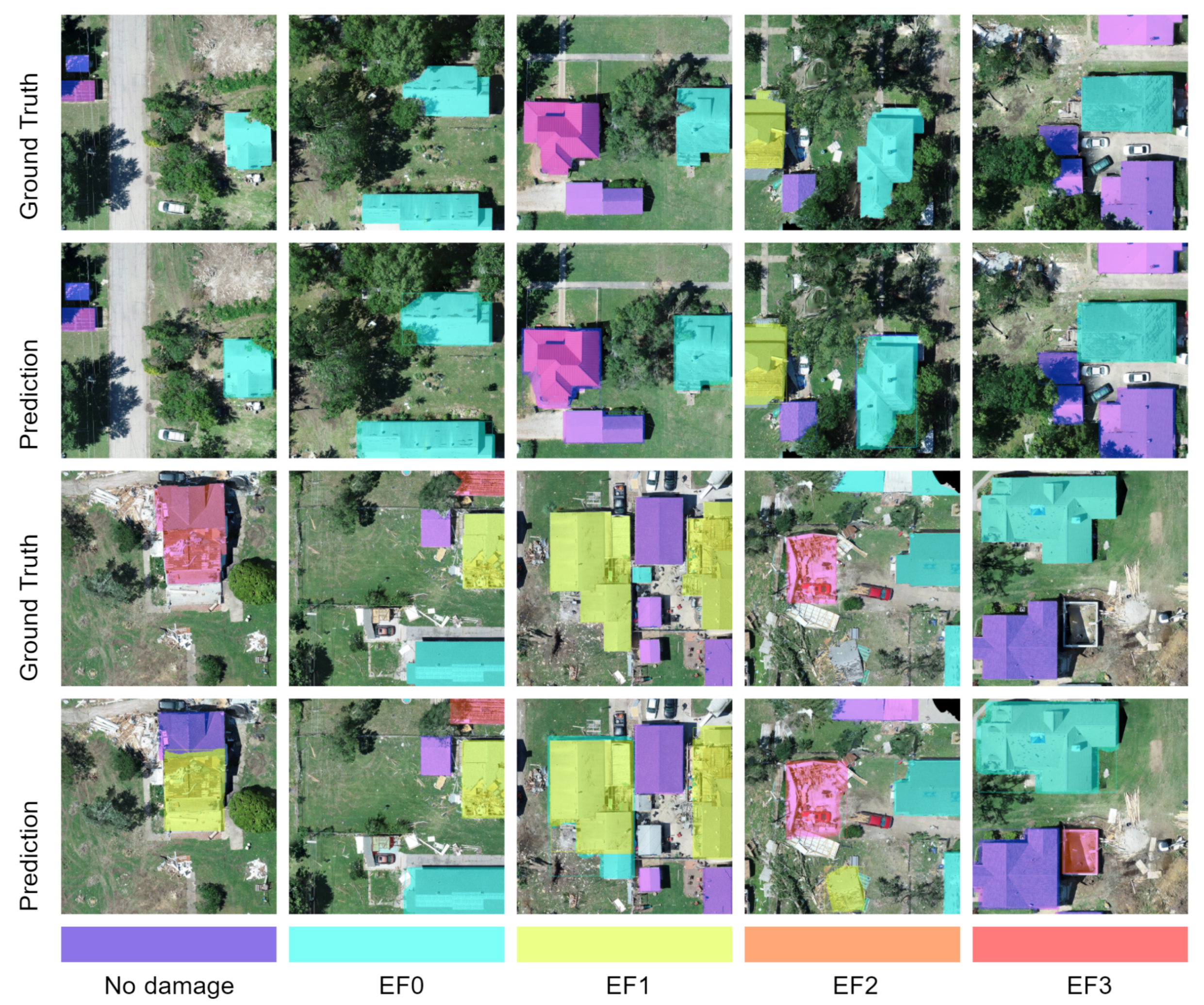
As presented in Table 5, the evaluation metrics for the object detection neural networks show good model performance. For binary object detection, the mAP for a list of IoU [0.5:0.95] was 59.1% on the validation dataset (103), and the mAP for other IoU thresholds (0.5 and 0.75) were even higher. Interestingly, the model without data augmentation for binary object detection narrowly outperformed the model with data augmentation by 0.2–2%. As a result, the binary object detection model without data augmentation was used to conduct inference on the test dataset (102), resulting in mAP(IoU = [0.5:0.95]) and mAR(IoU = [0.5:0.95]) values of 48.2% and 63.3%, respectively. For multi-class object detection, data augmentation improved model performance and therefore was used to conduct inference on the test dataset. The evaluation metrics for multi-class object detection, although lower than binary object detection, also show good model performance with mAP(IoU = [0.5:0.95]) and mAR(IoU = [0.5:0.95]) values of 35.7% and 45.3%, respectively, on the test dataset. Examples of multi-class object detection inference and ground truth from the validation and test datasets are presented in Figure 5.
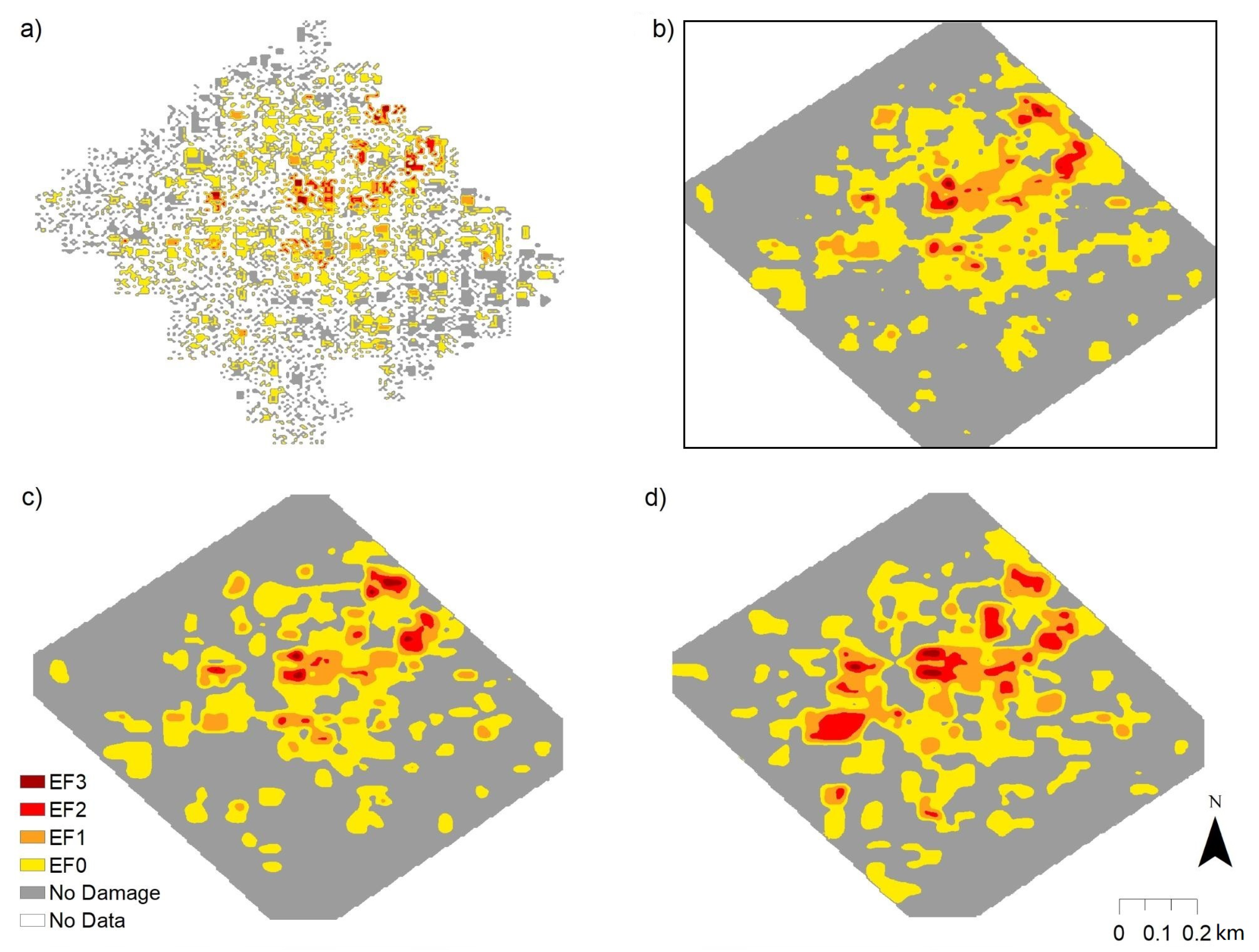
Figure 6 shows good agreement between the neural network inference and ground-truth heatmaps for object detection. For binary object detection, the DNN detected most damaged structures as evidenced by the concentration of damaged structures near the center in the inference heatmap (Figure 6a), compared with the ground truth (Figure 6b). Only minor differences in building footprints were observed in the western and southern portions (Figure 6a,b), pointing to some issues related to the binary object detection. For multi-class object detection, although the damage of a few buildings was underestimated, good agreement in damage trends is shown in Figure 6c,d. Both the multi-class object detection inference (Figure 6c) and ground truth (Figure 6d) show major structural damage (EF2/EF3) located near the center and minor structural damage (EF0/EF1) surrounding most of the area.

3.2. Neural Network Image Classification

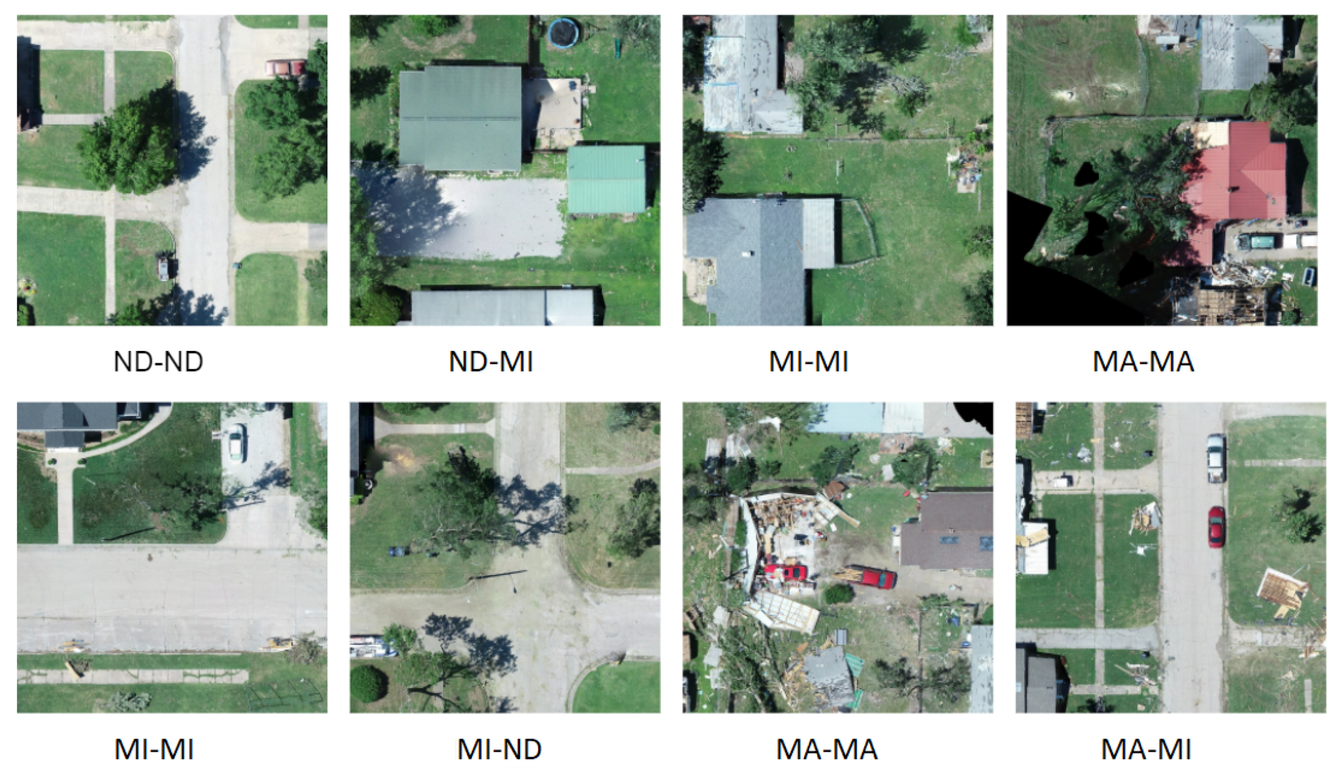
Table 6 shows the image classification accuracy for the state-of-the-art image classification neural networks used in this research. For binary damage classification, DenseNet-161 [40] had the best performance on the validation dataset with an accuracy of 84.8%. Therefore, for the test dataset, DenseNet-161 was used to conduct inference, yielding very high accuracy (84.0%). For multi-class classification, ResNeXt-101 [39] had the best performance on the validation dataset, with an accuracy of 81.5%, and reached an accuracy of 74.0% on the test dataset. Examples of multi-class image classification inference and ground truth from the validation and test datasets are shown in Figure 7.
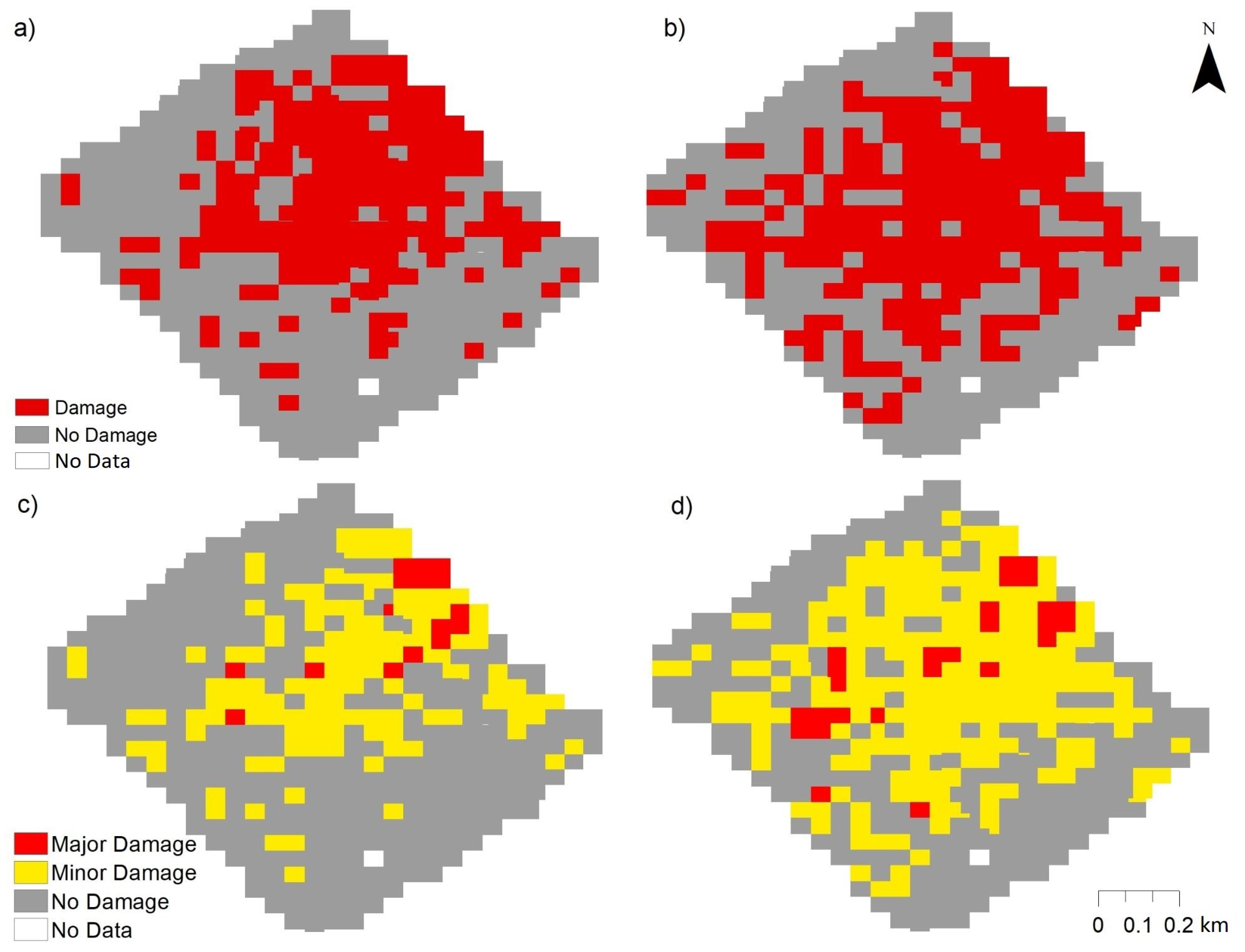
From the heatmaps (Figure 8), the DNNs also showed good performance for tornado damage classification. For binary damage classification, the DNN classified most of the damaged features relative to the ground truth (Figure 8a,b). However, in the western part, some tornado damage was underestimated especially near the edge (Figure 8a,b). For multi-class image classification, the DNN captured the overall trend with clusters of major damage (red pixels) near the center of the damage path (Figure 8c,d). There was a slight underestimation of major damage near the western part, but overall, the image classification performed well in estimating tornado damage (Figure 8c,d).

3.3. Gaussian Process Regression

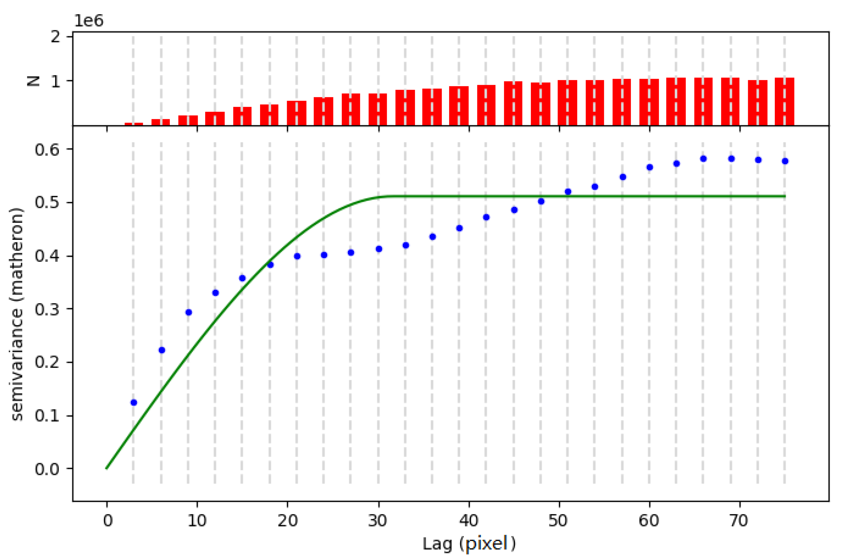
The spatial autocorrelation of one GP training dataset is shown in the semivariogram (Figure 9). The approximated spherical model (green curve) shows that within a certain range of separation distance, the sample semivariance increases with the distance to other samples, which implies that near tornado damage is more related than distant tornado damage and thus supports that the GP regression is appropriate in this study.
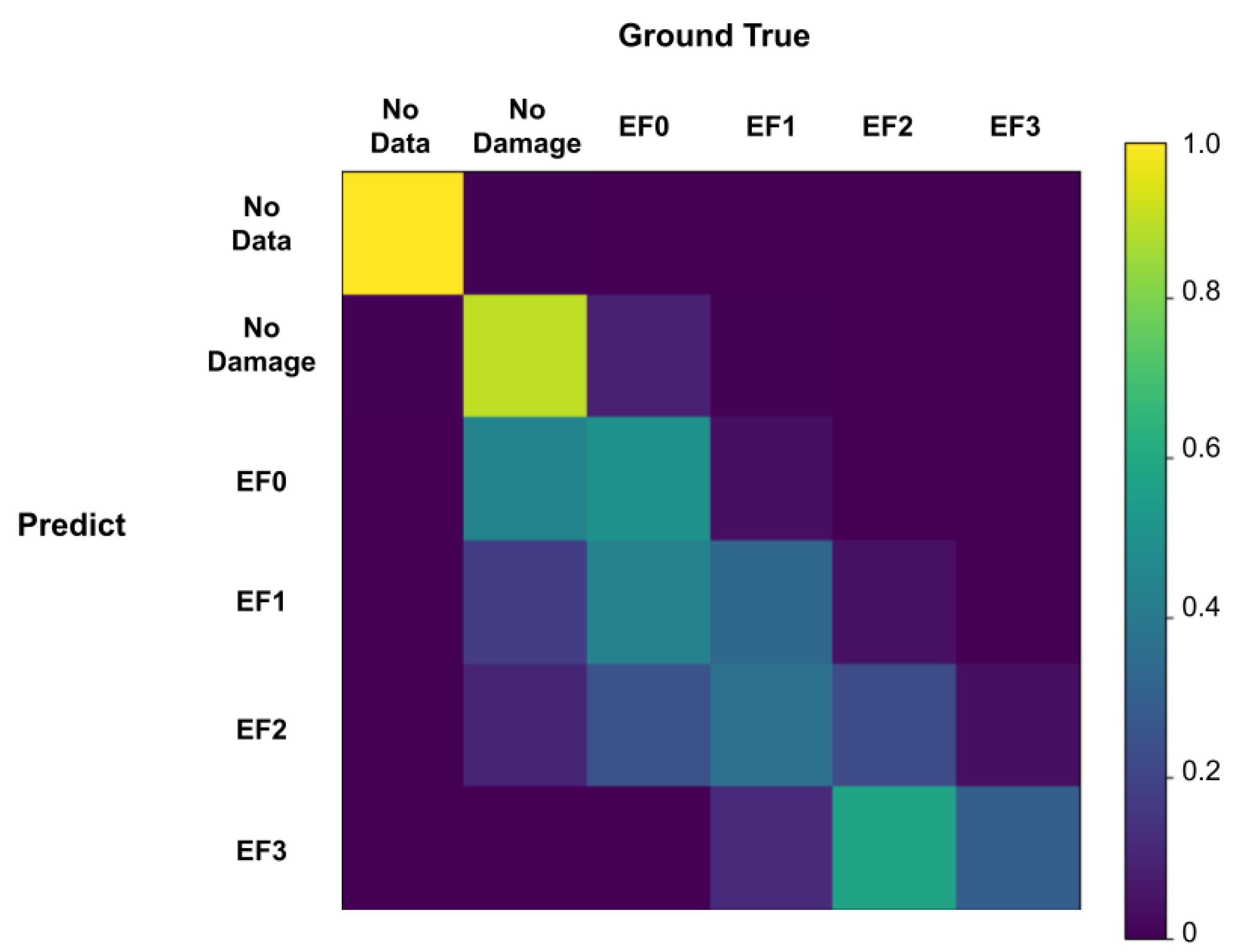
Figure 10a shows one of the GP training dataset samples from neural network inference, and the corresponding tornado damage heatmap from the GP inference is shown in Figure 10b. The GP regression results from neural network inference captured the variability and location of tornado damage similar to those observed in the ground truth (Figure 10c,d). The GP regression results from neural network inference showed only minor differences in the amount of EF3 damage, underestimating some of the EF3 damage near the western area. Despite these minor differences, the GP regression results from neural network inference best captured the different magnitudes of damage, including no damage, with the RMSD of 0.18 between the averaged GP regression rasters (Section 2.5.4). The normalized confusion matrix (Figure 11) also shows good agreement between the averaged-and-discretized GP regression rasters from neural network inference and ground-truth annotations. Although there are certain damage underestimates on EF1, EF2, and EF3 in the normalized confusion matrix, the elements in the matrix reside tightly along the diagonal, indicating relatively small errors between predictions and ground truth.
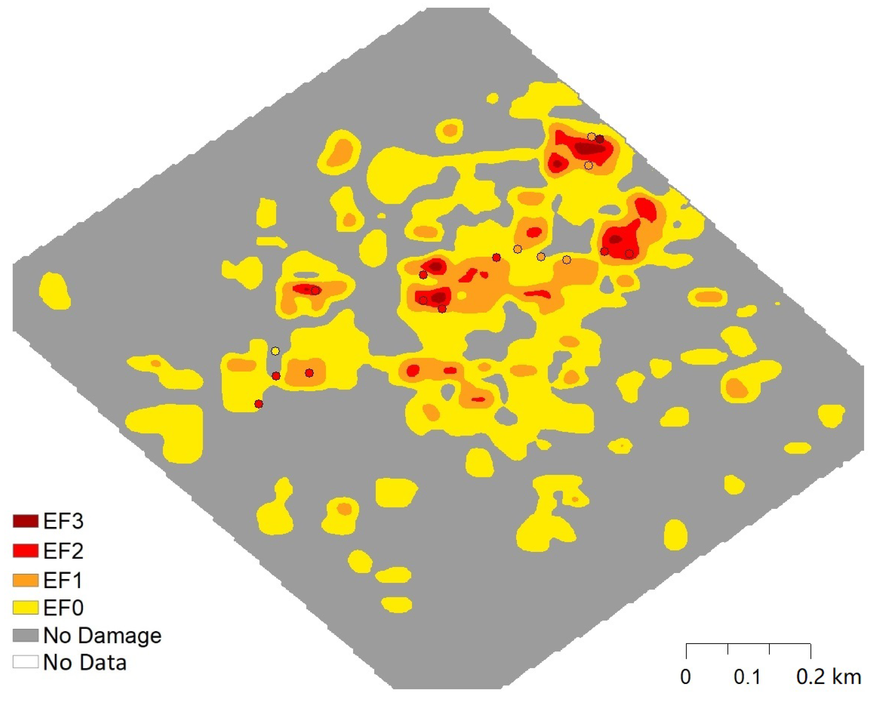
As illustrated in Figure 12, the overlay shows relatively good agreement between the GP regression heatmap from neural network inference and NWS ground survey data. EF-scale estimates from GP regression closely align with NWS EF-scale ratings with higher damage ratings near the center. A few differences exist between EF-scale ratings assigned by NWS and estimations from GP regression. However, most of these differences occur along damage gradients, where EF-scale estimates decrease by one or more damage ratings.

4. Discussion

This study presented data-driven approaches to automate tornado damage estimation based on SfM orthomosaics (~2 cm/pixel) generated from UAS surveys from the EF3-scale tornado that hit Eureka, Kansas, on 26 June 2018. We applied DNNs to estimate tornado damage in four scenarios: (1) object detection with binary categories, (2) object detection with multiple categories, (3) image classification with binary categories, and (4) image classification with multiple categories. Our results show good inference performance with object detection and image classification according to Table 5 and Table 6, illustrating the ability to automate tornado damage estimation. Both object detection and image classification approaches have their advantages in tornado damage estimation. The object detection provides higher-resolution damage estimates, and the image classification enables faster damage estimation due to less time required for data annotation.
Solutions to imbalanced training datasets have been investigated in this paper. Binary-class damage estimation for both object detection and image classification resulted in better performance than multi-class damage estimation because the binarized datasets are more balanced. We also applied data augmentation to compensate for the imbalanced training datasets. However, data augmentation alone may be insufficient in addressing imbalanced training datasets since only a slight improvement was shown on binary-class object detection.
This study is one of the first to accurately depict geolocations of tornado damage estimates using tornado damage heatmaps. The first type of tornado damage heatmap was generated by stitching inference results from the DNNs. The second type of tornado damage heatmap was produced using a GP regression model based on both object detection and image classification inference results. The GP regression not only demonstrated good performance with an RMSD of 0.18, but also captured similar damage trends when compared with NWS ground survey data (Figure 12). This finding illustrates how the GP regression can capture damage variability, which could help NWS WFOs refine their damage assessments in a desktop environment. Specifically, spatially continuous damage information can be used to generate EF-scale contours and better understand high-wind impacts. Additionally, providing spatially explicit tornado damage estimates can lead to better decision-making with regard to disaster response and recovery.
While the GP regression heatmap provides spatially continuous damage information, the GP regression results could have been affected by the DNN inference results. This is because the input of the GP regression model was based on inference results from the DNNs. The coupling between the DNNs and GP regression could partially explain the similar trend of underestimated damage observed in the object detection heatmap (Figure 6c) and GP regression heatmap (Figure 10c). Therefore, future work should examine how error and uncertainty in the DNN outputs propagate through the GP regression and affect the results of the tornado damage heatmaps.
Future work should build more balanced datasets to improve the performance of data-driven approaches to tornado damage estimation. First, underestimation of tornado damage from the neural networks correlates with the imbalanced training datasets where there are more “no damage” data points than other categories. Second, we have shown binary-class object detection and image classification, whose training datasets are more balanced, resulting in better performance than multi-class scenarios. This finding also indicates the effectiveness of a more balanced dataset. Third, we only had three categories for image classification and thus introduced a lookup table to convert these three categories to numeric labels based on EF-scale ratings. We have not studied how the errors introduced from the conversion could affect the GP regression results. These uncertainties could be eliminated as balanced training datasets become available for image classification. These datasets should also include higher-end EF scale damage to capture the range of tornado damage. We believe that building balanced datasets is key to improving such data-driven approaches for tornado damage estimation and other high-wind damage assessments. Additionally, algorithmic approaches [29] to the imbalanced dataset problem should also be investigated in future work.

5. Conclusions

This study explored data-driven approaches for tornado damage estimation based on SfM orthomosaics from UAS imagery using both object detection and image classification neural networks. We also produced two types of tornado damage heatmaps that accurately depict geolocations of tornado damage estimates. Generally, the data-driven approaches used in this study (object detection, image classification, and GP regression) all demonstrated good performance in tornado damage estimation based on relatively high evaluation metrics and good correlation with NWS ground survey data. Each approach has its advantages. Specifically, object detection neural networks (e.g., residential building damage) can produce detailed tornado damage estimates, which can assist insurance companies and emergency managers in calculating economic losses. Image classification neural networks can provide rapid tornado estimation because of the lower time required for data annotation. Such timely information could help emergency managers and other decision-makers with disaster response and recovery. Lastly, tornado damage heatmaps produced from GP regression results can provide spatially continuous tornado damage estimates. This spatially continuous dataset can help NWS WFOs and emergency managers with detailed damage assessments. While our work has investigated DL approaches for tornado damage estimation using 2D visible orthomosaics, the Mask R-CNN architecture (based on 2D CNNs) can be easily extended to other applications with additional information (e.g., multispectral orthomosaics, digital elevation models), as demonstrated by Chen et al. [35].

Author Contributions

Conceptualization, Z.C. and M.W.; methodology, Z.C.; data collection, M.W. and R.K.D.; data annotation, M.W.; software, Z.C.; validation, Z.C. and M.W.; writing—original draft preparation, Z.C. and M.W.; writing—review and editing, Z.C., M.W., J.D., R.K.D. and R.S.C. All authors have read and agreed to the published version of the manuscript.

Funding

This research received no external funding.

Institutional Review Board Statement

Not applicable.

Informed Consent Statement

Not applicable.

Data Availability Statement

The code for this study is available on Github (https://github.com/ZhiangChen/tornado_ML; accessed on 18 April 2021). The image data in this study contains sensitive residential information, and will be made available on request.

Conflicts of Interest

The authors declare no conflict of interest.

Abbreviations

The following abbreviations are used in this manuscript:
CNNConvolutional Neural Network
DLDeep Learning
DNN           Deep Neural Network
EFEnhanced Fujita
FCNFully Convolutional Network
GCPGround Control Point
GNSSGlobal Navigation Satellite System
GPGaussian Process
IoUIntersection over Union
MAMajor Damage
mAPmean Average Precision
mARmean Average Recall
MIMinor Damage
NDNo Damage
NWSNational Weather Service
NWS WFONational Weather Service Weather Forecast Office
PFNPyramid Feature Network
RMSDRoot-Mean-Square Deviation
SfMStructure from Motion
UASUnpolited Aerial System

Appendix A

The orthomosaics in this study were structured from four different, subsequent UAS surveys. In spite of geological overlaps between the adjacent sections, the SfM orthomosaics on the overlap areas are different because of lighting conditions, SfM artifacts, and data preparation. Orthomosaic samples on the overlap areas are shown in Figure A1.
Figure A1. Orthomosaic samples on overlap areas: (a) 101, (b) 102, (c) 103, and (d) 104.
Remotesensing 13 01669 g0a1
Many features distinguish Figure A1a,b from two orthomosaics at the same location: (1) there is no car at the right bottom corner in Figure A1a; (2) the right side of the building in Figure A1a is distorted at the edge of SfM orthomosaic; (3) the color in Figure A1a is slightly cooler; and (4) the right top corner in Figure A1a is blank because of SfM. The different shadows between Figure A1c,d show the changing lighting conditions.
Additionally, splitting the orthomosaics in data preparation shifted features on the image tiles. For example, a house at the center of an image tile from 101 might be at the bottom of an image tile from 102. To conclude, even though geological overlaps exist between the survey sections, the features on SfM orthomosaics are different on the overlap area. Therefore, we believe the effects of such geological overlaps on the deep learning evaluation should be insignificant.

Appendix B

The GP kernel parameters, such as the noise variance σ n 2 , kernel function length scale l, and signal variance σ f 2 , are referred to as the GP hyperparameters because they are parameters of a non-parametric model and can be learned from training using optimization methods. The DL hyperparameters usually refer to the parameters determining the neural network structure and the parameters determining the optimization methods for the neural network training. In spite of recent research in meta learning, the DL hyperparameters are usually set before training.

References

  1. Edwards, R.; LaDue, J.G.; Ferree, J.T.; Scharfenberg, K.; Maier, C.; Coulbourne, W.L. Tornado intensity estimation: Past, present, and future. Bull. Am. Meteorol. Soc. 2013, 94, 641–653. [Google Scholar] [CrossRef]
  2. Center for Disaster Philanthropy—Tornadoes. Available online: https://disasterphilanthropy.org/issue-insight/tornadoes/ (accessed on 4 January 2020).
  3. Changnon, S.A. Tornado losses in the United States. Nat. Hazards Rev. 2009, 10, 145–150. [Google Scholar] [CrossRef]
  4. Doswell, C.A., III; Brooks, H.E.; Dotzek, N. On the implementation of the enhanced Fujita scale in the USA. Atmos. Res. 2009, 93, 554–563. [Google Scholar] [CrossRef] [Green Version]
  5. Giordan, D.; Manconi, A.; Remondino, F.; Nex, F. Use of unmanned aerial vehicles in monitoring application and management of natural hazards. Geomat. Natl. Hazards Risk 2017, 8, 1–4. [Google Scholar] [CrossRef]
  6. Myint, S.W.; Yuan, M.; Cerveny, R.S.; Giri, C.P. Comparison of remote sensing image processing techniques to identify tornado damage areas from Landsat TM data. Sensors 2008, 8, 1128–1156. [Google Scholar] [CrossRef] [Green Version]
  7. Wang, W.; Qu, J.J.; Hao, X.; Liu, Y.; Stanturf, J.A. Post-hurricane forest damage assessment using satellite remote sensing. Agric. For. Meteorol. 2010, 150, 122–132. [Google Scholar] [CrossRef]
  8. Wagner, M.; Doe, R.K.; Johnson, A.; Chen, Z.; Das, J.; Cerveny, R.S. Unpiloted aerial systems (UASs) application for tornado damage surveys: Benefits and procedures. Bull. Am. Meteorol. Soc. 2019, 100, 2405–2409. [Google Scholar] [CrossRef]
  9. Diaz, J.; Joseph, M.B. Predicting property damage from tornadoes with zero-inflated neural networks. Weather Clim. Extrem. 2019, 25, 100216. [Google Scholar] [CrossRef]
  10. Le, V.; Caracoglia, L. A neural network surrogate model for the performance assessment of a vertical structure subjected to non-stationary, tornadic wind loads. Comput. Struct. 2020, 231, 106208. [Google Scholar] [CrossRef]
  11. He, K.; Zhang, X.; Ren, S.; Sun, J. Deep residual learning for image recognition. In Proceedings of the IEEE Conference on Computer Vision and Pattern Recognition, Las Vegas, NV, USA, 26 June–1 July 2016; pp. 770–778. [Google Scholar]
  12. Ronneberger, O.; Fischer, P.; Brox, T. U-net: Convolutional networks for biomedical image segmentation. In Proceedings of the International Conference on Medical image computing and computer-assisted intervention, Munich, Germany, 5–9 October 2015; pp. 234–241. [Google Scholar]
  13. He, K.; Gkioxari, G.; Dollár, P.; Girshick, R. Mask R-CNN. In Proceedings of the IEEE International Conference on Computer Vision, Venice, Italy, 22–29 October 2017; pp. 2961–2969. [Google Scholar]
  14. Vakalopoulou, M.; Karantzalos, K.; Komodakis, N.; Paragios, N. Building detection in very high resolution multispectral data with deep learning features. In Proceedings of the 2015 IEEE International Geoscience and Remote Sensing Symposium (IGARSS), Milan, Italy, 26–31 July 2015; pp. 1873–1876. [Google Scholar]
  15. Abdollahi, A.; Pradhan, B.; Alamri, A.M. An ensemble architecture of deep convolutional Segnet and Unet networks for building semantic segmentation from high-resolution aerial images. Geocarto Int. 2020, 1–16. [Google Scholar] [CrossRef]
  16. Sony, S.; Dunphy, K.; Sadhu, A.; Capretz, M. A systematic review of convolutional neural network-based structural condition assessment techniques. Eng. Struct. 2021, 226, 111347. [Google Scholar] [CrossRef]
  17. Pi, Y.; Nath, N.D.; Behzadan, A.H. Convolutional neural networks for object detection in aerial imagery for disaster response and recovery. Adv. Eng. Informatics 2020, 43, 101009. [Google Scholar] [CrossRef]
  18. Cao, Q.D.; Choe, Y. Post-Hurricane Damage Assessment Using Satellite Imagery and Geolocation Features. arXiv 2020, arXiv:2012.08624. [Google Scholar]
  19. Kakareko, G.; Jung, S.; Ozguven, E.E. Estimation of tree failure consequences due to high winds using convolutional neural networks. Int. J. Remote Sens. 2020, 41, 9039–9063. [Google Scholar] [CrossRef]
  20. Kocatepe, A.; Ulak, M.B.; Kakareko, G.; Ozguven, E.E.; Jung, S.; Arghandeh, R. Measuring the accessibility of critical facilities in the presence of hurricane-related roadway closures and an approach for predicting future roadway disruptions. Nat. Hazards 2019, 95, 615–635. [Google Scholar] [CrossRef]
  21. Li, Y.; Ye, S.; Bartoli, I. Semisupervised classification of hurricane damage from postevent aerial imagery using deep learning. J. Appl. Remote Sens. 2018, 12, 045008. [Google Scholar] [CrossRef]
  22. Abdollahi, A.; Pradhan, B.; Gite, S.; Alamri, A. Building footprint extraction from high resolution aerial images using Generative Adversarial Network (GAN) architecture. IEEE Access 2020, 8, 209517–209527. [Google Scholar] [CrossRef]
  23. Cheng, C.S.; Behzadan, A.H.; Noshadravan, A. Deep learning for post-hurricane aerial damage assessment of buildings. Comput.-Aided Civ. Infrastruct. Eng. 2020. [Google Scholar] [CrossRef]
  24. Kerle, N.; Nex, F.; Gerke, M.; Duarte, D.; Vetrivel, A. UAV-based structural damage mapping: A review. ISPRS Int. J. Geo-Inf. 2020, 9, 14. [Google Scholar] [CrossRef] [Green Version]
  25. Duarte, D.; Nex, F.; Kerle, N.; Vosselman, G. Satellite image classification of building damages using airborne and satellite image samples in a deep learning approach. ISPRS Ann. Photogramm. Remote Sens. Spat. Inf. Sci. 2018, 4, 89–96. [Google Scholar] [CrossRef] [Green Version]
  26. Nex, F.; Duarte, D.; Tonolo, F.G.; Kerle, N. Structural building damage detection with deep learning: Assessment of a state-of-the-art CNN in operational conditions. Remote Sens. 2019, 11, 2765. [Google Scholar] [CrossRef] [Green Version]
  27. Mohammadi, M.E.; Watson, D.P.; Wood, R.L. Deep learning-based damage detection from aerial SfM point clouds. Drones 2019, 3, 68. [Google Scholar] [CrossRef] [Green Version]
  28. Liao, Y.; Mohammadi, M.E.; Wood, R.L. Deep learning classification of 2D orthomosaic images and 3D point clouds for post-event structural damage assessment. Drones 2020, 4, 24. [Google Scholar] [CrossRef]
  29. Krawczyk, B. Learning from imbalanced data: Open challenges and future directions. Prog. Artif. Intell. 2016, 5, 221–232. [Google Scholar] [CrossRef] [Green Version]
  30. National Centers for Environmental Information. Available online: https://www.ncdc.noaa.gov/stormevents/eventdetails.jsp?id=757551 (accessed on 11 November 2018).
  31. Westoby, M.J.; Brasington, J.; Glasser, N.F.; Hambrey, M.J.; Reynolds, J.M. ’Structure-from-Motion’ photogrammetry: A low-cost, effective tool for geoscience applications. Geomorphology 2012, 179, 300–314. [Google Scholar] [CrossRef] [Green Version]
  32. NOAA Damage Assessment Toolkit. Available online: https://apps.dat.noaa.gov/StormDamage/DamageViewer/ (accessed on 5 January 2021).
  33. Agisoft. Available online: https://www.agisoft.com/ (accessed on 8 May 2020).
  34. Johnson, K.; Nissen, E.; Saripalli, S.; Arrowsmith, J.R.; McGarey, P.; Scharer, K.; Williams, P.; Blisniuk, K. Rapid mapping of ultrafine fault zone topography with structure from motion. Geosphere 2014, 10, 969–986. [Google Scholar] [CrossRef]
  35. Chen, Z.; Scott, T.R.; Bearman, S.; Anand, H.; Keating, D.; Scott, C.; Arrowsmith, J.R.; Das, J. Geomorphological analysis using unpiloted aircraft systems, structure from motion, and deep learning. In Proceedings of the 2020 IEEE/RSJ International Conference on Intelligent Robots and Systems (IROS), Las Vegas, NV, USA, 25–29 October 2020; pp. 1276–1283. [Google Scholar]
  36. Labelbox. Available online: https://labelbox.com/ (accessed on 25 May 2020).
  37. Lin, T.Y.; Dollár, P.; Girshick, R.; He, K.; Hariharan, B.; Belongie, S. Feature pyramid networks for object detection. In Proceedings of the IEEE Conference on Computer Vision and Pattern Recognition, Honolulu, HI, USA, 21–26 July 2017; pp. 2117–2125. [Google Scholar]
  38. Zagoruyko, S.; Komodakis, N. Wide residual networks. arXiv 2016, arXiv:1605.07146. [Google Scholar]
  39. Xie, S.; Girshick, R.; Dollár, P.; Tu, Z.; He, K. Aggregated residual transformations for deep neural networks. In Proceedings of the IEEE Conference on Computer Vision and Pattern Recognition, Honolulu, HI, USA, 21–26 July 2017; pp. 1492–1500. [Google Scholar]
  40. Huang, G.; Liu, Z.; Van Der Maaten, L.; Weinberger, K.Q. Densely connected convolutional networks. In Proceedings of the IEEE Conference on Computer Vision and Pattern Recognition, Honolulu, HI, USA, 21–26 July 2017; pp. 4700–4708. [Google Scholar]
  41. Marcel, S.; Rodriguez, Y. Torchvision the machine-vision package of torch. In Proceedings of the 18th ACM International Conference on Multimedia, Firenze, Italy, 25–29 October 2010; pp. 1485–1488. [Google Scholar]
  42. Lin, T.Y.; Maire, M.; Belongie, S.; Hays, J.; Perona, P.; Ramanan, D.; Dollár, P.; Zitnick, C.L. Microsoft coco: Common objects in context. In Proceedings of the European Conference on Computer Vision, Zurich, Switzerland, 6–12 September 2014; pp. 740–755. [Google Scholar]
  43. Deng, J.; Dong, W.; Socher, R.; Li, L.-J.; Li, K.; Li, F. Imagenet: A large-scale hierarchical image database. In Proceedings of the 2009 IEEE Conference on Computer Vision and Pattern Recognition, Miami, FL, USA, 20–25 June 2009; pp. 248–255. [Google Scholar]
  44. Rasmussen, C.E.; Williams, C.K.I. Gaussian Processes in Machine Learning; MIT Press: Cambridge, MA, USA, 2005. [Google Scholar]
  45. Gardner, J.R.; Pleiss, G.; Bindel, D.; Weinberger, K.Q.; Wilson, A.G. Gpytorch: Blackbox matrix-matrix gaussian process inference with gpu acceleration. arXiv 2018, arXiv:1809.11165. [Google Scholar]
  46. Bentley, J.L. Multidimensional binary search trees used for associative searching. Commun. ACM 1975, 18, 509–517. [Google Scholar] [CrossRef]
  47. Scikit-Learn: Sklearn.metrics.confusion_matrix. Available online: https://scikit-learn.org/stable/modules/generated/sklearn.metrics.confusion_matrix.html (accessed on 15 February 2021).
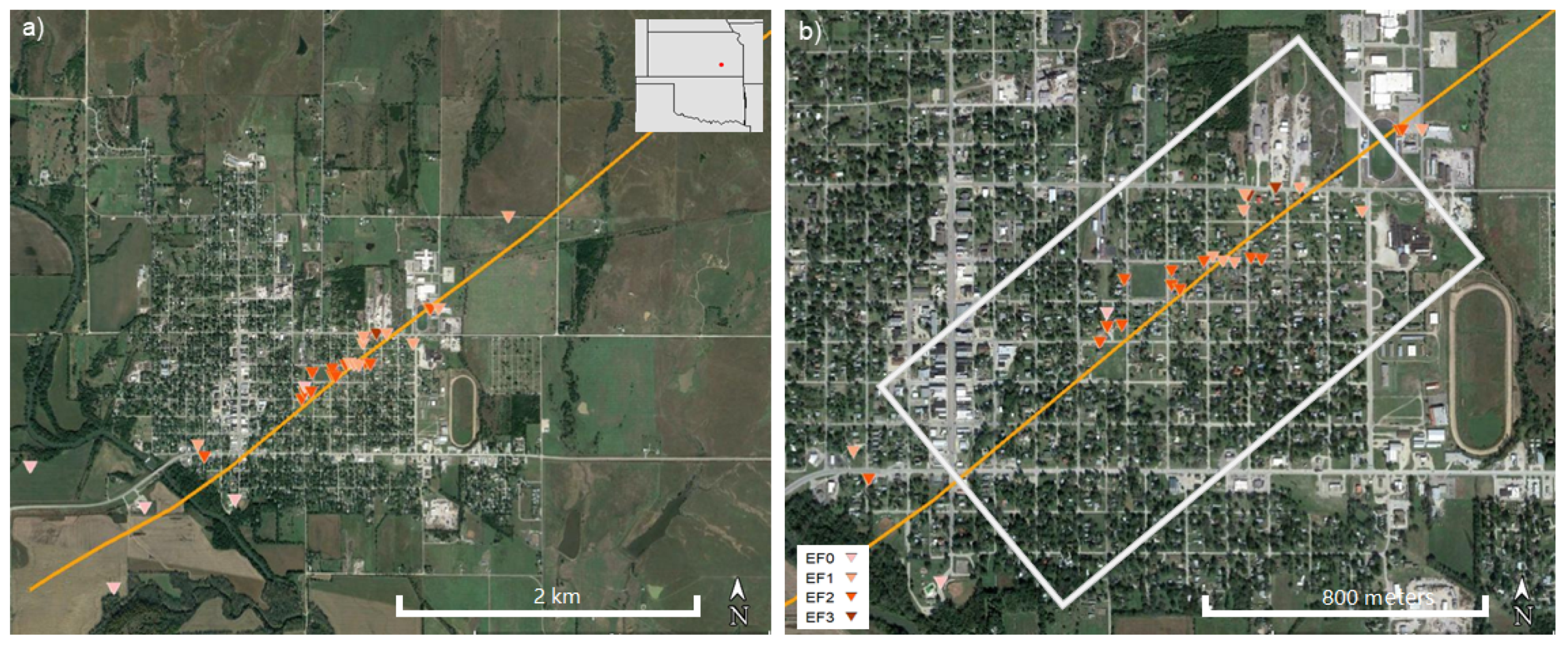
Figure 1. Kansas tornado, 26 June 2018 Eureka, (a) path overview and (b) survey site outlined in white box. Inverted triangles correspond to Enhanced Fujita (EF) scale ratings with the strongest damage (EF3) shown in dark red and weakest damage (EF0) shown in light pink were obtained from ground surveys conducted by the National Weather Service Weather Forecast Offices (NWS WFOs) Wichita, Kansas.
Remotesensing 13 01669 g001
Figure 2. UAS-based orthomosaics were used for training, validating, and testing neural networks. sections 101 and 104 (outlined in cyan) were used for training; section 103 (outlined in magenta) was used for validating; and section 102 (outlined in yellow) was used for testing.
Remotesensing 13 01669 g002
Figure 3. Workflow diagrams of (a) deep learning and (b) Gaussian process (GP) regression.
Remotesensing 13 01669 g003
Figure 4. Annotation data size summary. For object detection (left), the unit is object number; for image classification, the unit is image number.
Remotesensing 13 01669 g004
Figure 5. Examples of neural network inference and ground truth for multi-class object detection from validation and test datasets. Original image tiles are overlaid with masks from prediction or ground truth.
Remotesensing 13 01669 g005
Figure 6. Tornado damage heatmaps from object detection. (a) binary inference results, (b) binary ground truth, (c) multi-class inference results, and (d) multi-class ground truth.
Remotesensing 13 01669 g006
Figure 7. Examples of neural network inference and ground truth for multi-class image classification from validation and test datasets. ND: no damage, MI: minor damage, and MA: major damage. The legend below every subfigure shows ground-truth label and prediction label; e.g., MI-ND means ground-truth annotation is minor damage and neural network classified the same tile as no damage.
Remotesensing 13 01669 g007
Figure 8. Tornado damage heatmaps from image classification: (a) binary inference results, (b) binary ground truth, (c) multi-class inference results, and (d) multi-class ground truth.
Remotesensing 13 01669 g008
Figure 9. Semivariogram. Horizontal axis is lag distance, also known as separation distance between data points, in pixels. Blue dots represent semivariances of the corresponding lag distances in GP training dataset. Green curve is a sphere model fitted with the semivariances (blue dots). Red bins are the number of data point pairs in the same lag distance category groups.
Remotesensing 13 01669 g009
Figure 10. (a) One sample of GP regression training datasets from neural network inference, including all valid points from multi-class object detection and 30% randomly sampled valid data points from multi-class image classification. (b) Tornado damage heatmap from GP regression using the GP training dataset (Figure 10a). The pixel-wise average of the multiple GP regression results from (c) neural network inference and (d) ground-truth annotations. The border provided in Figure 10b is applicable to all other heatmaps; however, it was not displayed to maintain clean visualization. The white areas within the border indicate “No Data”.
Remotesensing 13 01669 g010
Figure 11. Normalized confusion matrix of averaged-and-discretized rasters. The elements are normalized over ground truth (rows) [47].
Remotesensing 13 01669 g011
Figure 12. Overlay between GP heatmap from neural network inference and NWS ground survey data points. Circles, which also show damage intensity according to EF scale, are ground-truth data obtained from NWS damage surveys.
Remotesensing 13 01669 g012
Table 1. Annotation rubric for classification.
Roof Cover FailureRoof Structure FailureDebrisTree
no damage<2%nosparsely scattered
and coverage <1%
minor broken branch
minor damage>2% and <50%nocoverage >1%major broken branch
or broken trunk or visible root
major damage>50%yes
Table 2. Lookup table to determine Y d .
R d No Data (0)No Damage (1)EF0 (2)EF1 (3)EF2 (4)EF3 (5)
Y d
R c
No Data (0)012345
No Damage (1)011.52.53.53.5
Minor Damage (2)01.5233.54
Major Damage (3)01.52.53.545
Table 3. Lookup table to determine Y c .
r d [0, 1.5)[1.5, 2)[2, 2.5)[2.5, 3)[3, 4)[4, 4.5)[4.5, 5]
Y c
R c
No Data (0)0
No Damage (1)(1+ r d )/21.5
Minor Damage (2)1.5 ( 2 + r d ) / 2 ( 3 + r d ) / 2 3.5
Major Damage (3)3.5 ( 4 + r d ) / 2 ( 5 + r d ) / 2
Table 4. EF scale discretization.
μ ^ (−inf, 0.5)[0.5, 1.5)[1.5, 2.5)[2.5, 3.5)[3.5, 4.5)[4.5, +inf)
EF ScaleNo DataNo DamageEF0EF1EF2EF3
Table 5. Evaluation metrics for binary and multi-class object detection.
SectionDetectionmAP(IoU = [0.5:0.95])mAP(IoU = 0.5)mAP(IoU = 0.75)mAR(IoU = [0.5:0.95])
103Binary59.1%74.3%66.0%73.2%
Augmented binary58.9%72.3%65.5%72.8%
Multi-class32.8%44.3%35.7%59.1%
Augmented multi-class36.1%48.5%37.9%52.8%
102Binary48.2%63.0%50.7%63.3%
Augmented multi-class35.7%42.8%39.6%45.3%
Table 6. Accuracy of binary and multi-class image classification.
SectionClassificationResNet-152Wide ResnNet-101ResNeXt-101DenseNet-161DenseNet-201
103Binary83.5%84.2%83.8%84.8%83.5%
Multi-class76.2%77.9%81.5%78.9%80.9%
102Binary 84.0%
Multi-class 74.0%
Publisher’s Note: MDPI stays neutral with regard to jurisdictional claims in published maps and institutional affiliations.