Evaporation Duct Height Nowcasting in China’s Yellow Sea Based on Deep Learning

Abstract

The evaporation duct is a weather phenomenon that often occurs in marine environments and affects the operation of shipborne radar. The most important evaluation parameter is the evaporation duct height (EDH). Forecasting the EDH and adjusting the working parameters and modes of the radar system in advance can greatly improve radar performance. Traditionally, short-term forecast methods have been used to estimate the EDH, which are characterized by low time resolution and poor forecast accuracy. In this study, a novel approach for EDH nowcasting is proposed based on the deep learning network and EDH data measured in the Yellow Sea, China. The factors that affect nowcasting were analyzed. The time resolution and forecast time were 5 min and 0–2 h, respectively. The results show that our proposed method has a higher forecast accuracy than traditional time series forecasting methods and confirm its feasibility and effectiveness.

1. Introduction

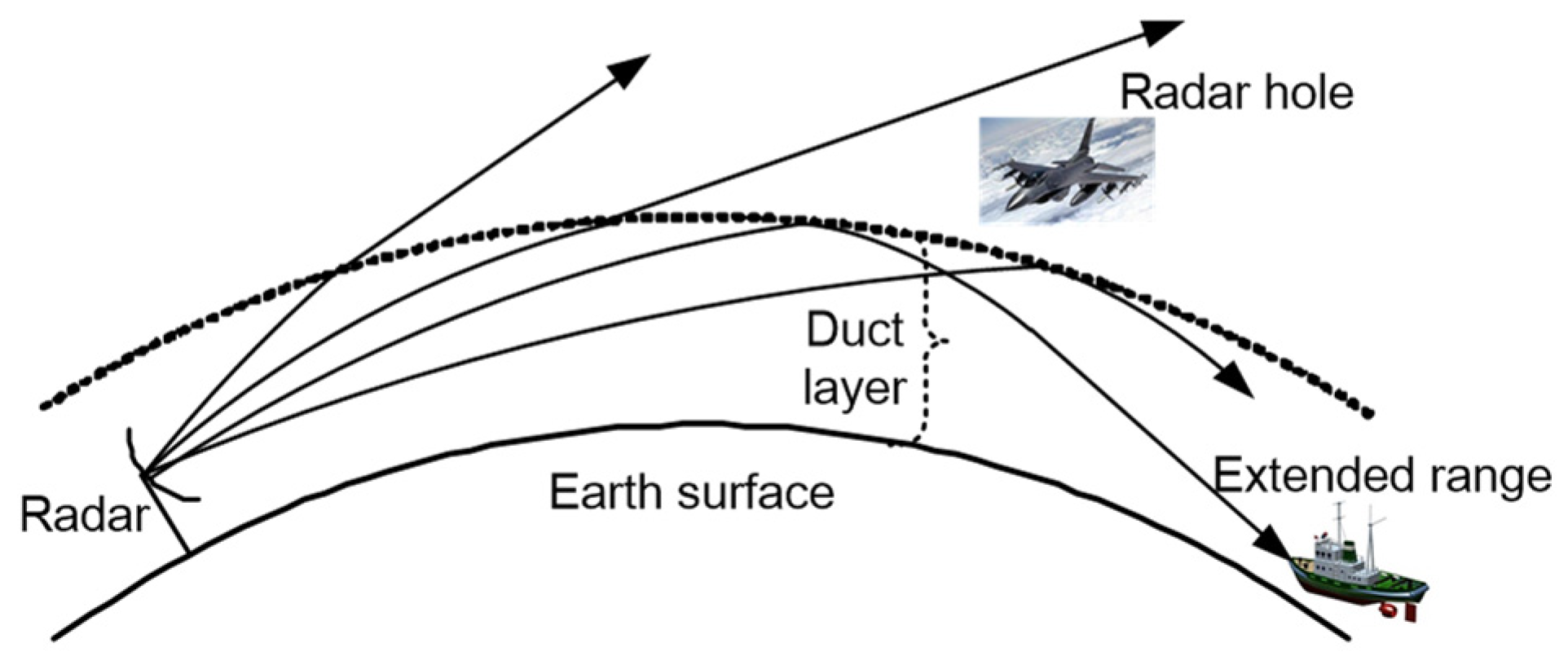
Evaporation ducts are atmospheric layers that form due to large-scale evaporation of seawater and are the most common type of duct in the air-sea boundary layer [1]. According to statistics, the probability of evaporation duct occurrence in the waters surrounding China is 85% [2,3]. An evaporation duct can change the propagation path and energy distribution of electromagnetic waves, which affects the system in microwave frequency band, such as radar systems, communication systems, etc. As shown in Figure 1, the main effects are as follows:

• Radar wave propagates with less propagation loss in an evaporation duct environment, which can lead to over-the-horizon detection such that more distant targets can be detected;
• Radar wave is bound by the evaporation duct layer, which leads to the formation of a blind area for radar detection.

Therefore, before the radar system is operated, the radar detection performance and detection area must be optimized to utilize beneficial effects, such as over-the-horizon detection, and avoid adverse effects, such as the detection of blind areas, to enhance the radar system performance. To predict the detection performance of a radar, it is necessary to first obtain evaporation duct height (EDH) data and process it with a radio wave propagation algorithm to calculate the radio wave propagation loss in different regions. Obtaining accurate evaporation duct forecasts is thus an important task.

At present, evaporation duct forecast data are mainly based on mesoscale numerical weather forecast models, such as the Weather Research and Forecasting model, which produce short-term forecasts. These methods mainly use global background data as their data sources, with a time resolution of 3 h, horizontal resolution of 0.25° × 0.25°, and forecast duration of 72–120 h. Limited by the temporal and spatial resolution of the background data, the temporal and the horizontal resolutions of the evaporation duct short-term forecast product are 1 h and 30 km × 30 km, respectively. These spatiotemporal resolutions cannot accurately reflect the short-term non-stationary change of the EDH and do not meet the needs of radar performance evaluation. Nowcasting duration is generally 0–2 h and the temporal resolution is at the minute-level or smaller; thus, it can better reflect the short-term change of the EDH, leading to a more accurate evaluation of the radar detection performance. Although the short-term forecasting and nowcasting of the EDH belong to the same category, the utilized models, methods, and data are different. Several studies have investigated short-term forecasting of the EDH and established numerous methods and models; however, there is a lack of research on nowcasting the EDH as well as on effective methods and models.

Although there is no mature nowcast model, several time series forecast methods can be used for nowcasting the EDH. In the 1980s, two types of methods were used for time series forecasting:

• Linear statistical methods;
• Nonlinear time series models such as the bilinear model [4] and autoregressive conditional heteroskedastic model [5].

Linear statistical methods yield better results for stable time series, but the results for unstable time series are poor [6,7]. Because the EDH is non-stationary, linear statistical methods are not suitable for its forecast. However, the decision tree, support vector machine (SVM), and nearest neighbor regression models that were developed [8,9], have poor forecast accuracy which needs to be further improved [10]. Deep learning was proposed by Hinton et al. [11] and can be used to solve nonlinear forecast problems. Deep learning has been applied to evaporation duct inversion, evaporation duct diagnosis, sea clutter time series prediction, and other fields, and have achieved good results. Guo et al. [12,13] realized the inversion of an evaporation duct using a deep learning network, which had a higher inversion accuracy than traditional methods. Zhu et al. [14] established an evaporation duct model using a deep learning network, which has a higher accuracy than the traditional Paulus-Jeske (P–J) model. Zhao et al. [15] used a long short-term memory (LSTM) model for long-distance sea clutter prediction. Based on previous research results, an approach to nowcast the EDH is proposed in this study.

The essence of deep learning is to use a large number of continuous EDH data to establish a deep learning network model with multiple hidden layers to learn the nonlinear mapping relationship between the measured and future EDH and improve forecast accuracy by optimizing the model parameters. The research results of this paper indicate that the EDH nowcasting model based on deep learning has better forecast accuracy than traditional methods.

The content of this paper is arranged as follows: the calculation method of the EDH and its variation characteristics are introduced in Section 2.1. The selection of the deep learning network is described in Section 2.2. The modeling method used for nowcasting the EDH based on the LSTM network is discussed in Section 2.3. In Section 3, the results of a comparative experiment are described, which show that the forecast accuracy of the proposed model is higher than that of traditional methods. In Section 4, different parameters affecting forecast performance are discussed. The conclusions are presented in Section 5.

2. Materials and Methods

2.1. Evaporation Duct Height Data

2.1.1. Calculation of the Evaporation Duct Height

Models that can be used to determine the evaporation duct mainly include the P–J model, Musson-Genon-Gauthier-Bruth model, and Babin models [16]. The P–J model is one of the most widely used models and has been integrated into the Integrated Reflection Effect Dissemination System [17]. The P–J model uses the air temperature, relative humidity, wind speed, atmospheric pressure, and sea surface temperature at a certain height from the sea surface as input parameters, introduces the potential refractive index as a similar parameter, and assumes that it satisfies the similarity theory [1]. The potential refractive index $N_p$ is calculated using the following Equation:

$$\frac{\partial {\mathrm{N}}_{\mathrm{p}}}{\partial z}=\frac{N_p\times \phi (\frac{z}{L})}{kz},$$

(1)

$$N_p=\frac{77.6}{\theta }\times (p+\frac{4810\times e_p}{\theta }),$$

(2)

where $z$, $L$, $k$, $p$, $\theta$, and $e_p$ are the height, the MoniObukhov length, the von Karmen’s constant, the atmospheric pressure, potential temperature, and water vapor pressure, respectively, and $N_p$ is the characteristic scale parameter of the pseudo-refractive index. The relationship between the potential refractive index and atmospheric refractive index satisfies the following condition [1]:

$$\frac{\partial N_p}{\partial z}\approx \frac{\partial N}{\partial z}+0.032,$$

(3)

where $N$ is the scaling parameter of potential refractivity. The evaporation duct appears when $\frac{\partial N_p}{\partial z}<-0.125$ [1]. The height corresponding to a vertical gradient of the potential refractive index that is equal to the critical value (−0.125) for the formation of an atmospheric duct is the EDH.

2.1.2. EDH Data Acquisition

From 2017 to 2019, an EDH data acquisition test was carried out in the Yellow Sea by the China Research Institute of Radiowave Propagation. The sensors used for the test included temperature, humidity, atmospheric pressure, wind speed, and sea surface temperature sensors. The sensor parameters are shown in

Table 1. Sensor parameters.

Sensor	Range	Accuracy	Resolution
Temperature	−35–60 ℃	±0.2 ℃	0.1 ℃
Relative humidity	0–100%	±5%	0.1%
Pressure	600–1100 hPa	±1 hPa	0.1 hPa
Wind speed	0–60 m/s	±2%	0.01 m/s
Sea surface temperature	−15–50 ℃	±0.3 ℃	0.1 ℃

.

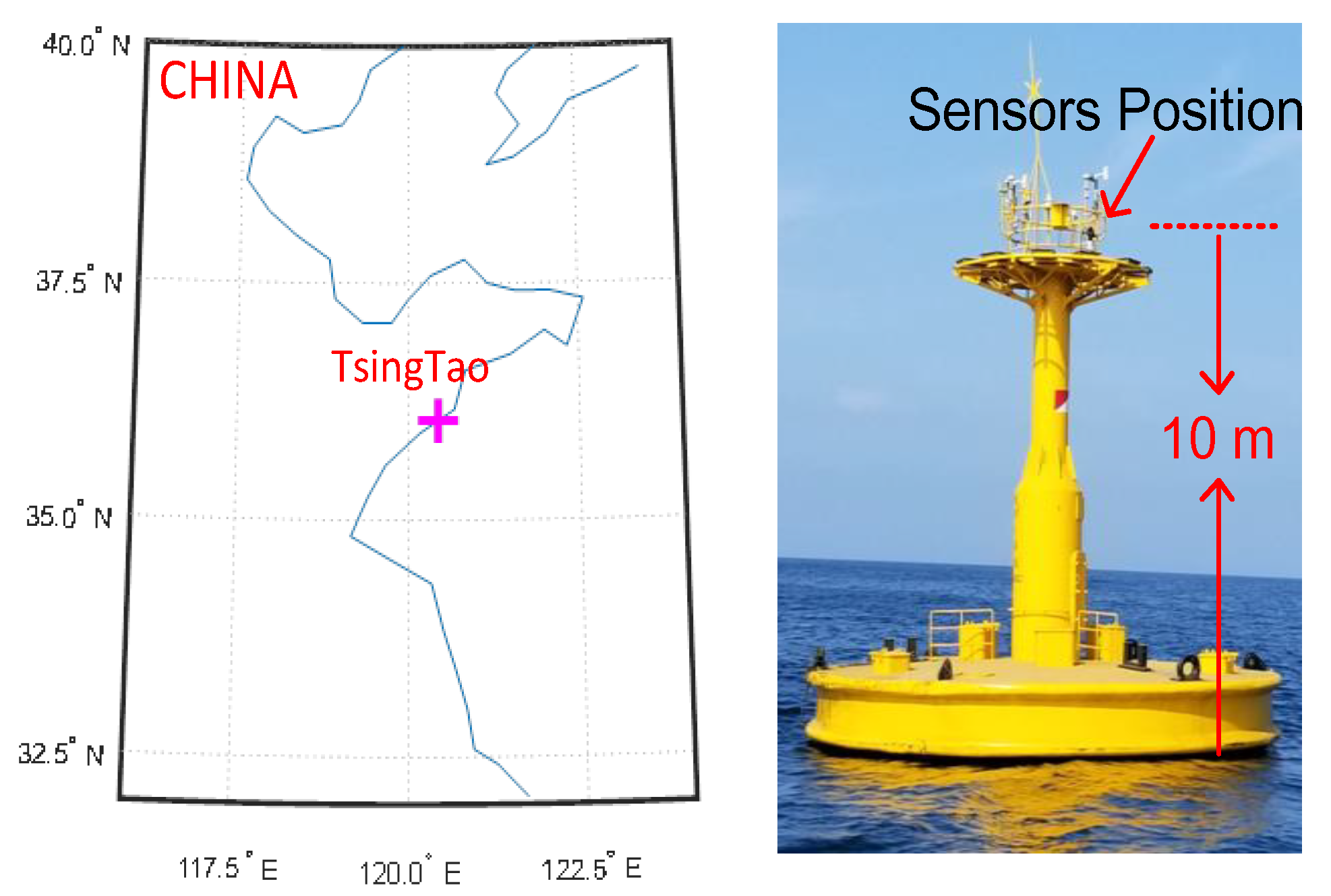
The above-mentioned sensors were installed on the top of the buoy, ~10 m away from the sea. The geographical location of the buoy and position of the sensor are shown in Figure 2.

Once the temperature, humidity, atmospheric pressure, wind speed, and sea surface temperature are obtained, the EDH can be calculated. If the wind speed is less than 0.01 knot, the EDH is set to zero. If not, the following four steps are taken [18].

• Step 1: calculate the bulk Richardson’s number
• Step 2: From the Richardson’s number, determine the Monin-Obukhov length
• Step 3: A potential refractivity difference between the air and the sea surface is determined from
• Step 4: The stability conditions are examined to determine which form the EDH equation will take

2.1.3. Variation of the EDH

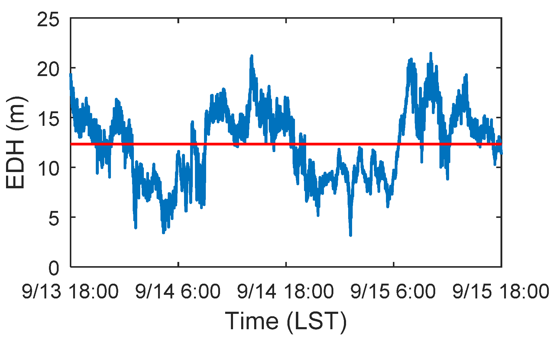
EDH data from 18:00 LST on 13 September to 18:00 LST on 15 September 2017 were selected for the analysis of the EDH variation. The daily variation of the EDH is shown in Figure 3.

Figure 3 shows that the height of the evaporation duct regularly changes during the selected time period. At night (from 13 September 18:00 to 14 September 6:00, from 14 September 18:00 to 15 September 6:00), the EDH is low, with a minimum of ~5 m; in the daytime (from 14 September 6:00 to 14 September 18:00, from 15 September 6:00 to 15 September 18:00), the EDH is higher, reaching up to 20 m. However, this change is not always constant and sometimes opposite to the change shown in the graph. It is certain that the EDH regularly changes, which is mainly controlled by the climate at the observation site. Based on this regular change, the EDH can be forecasted.

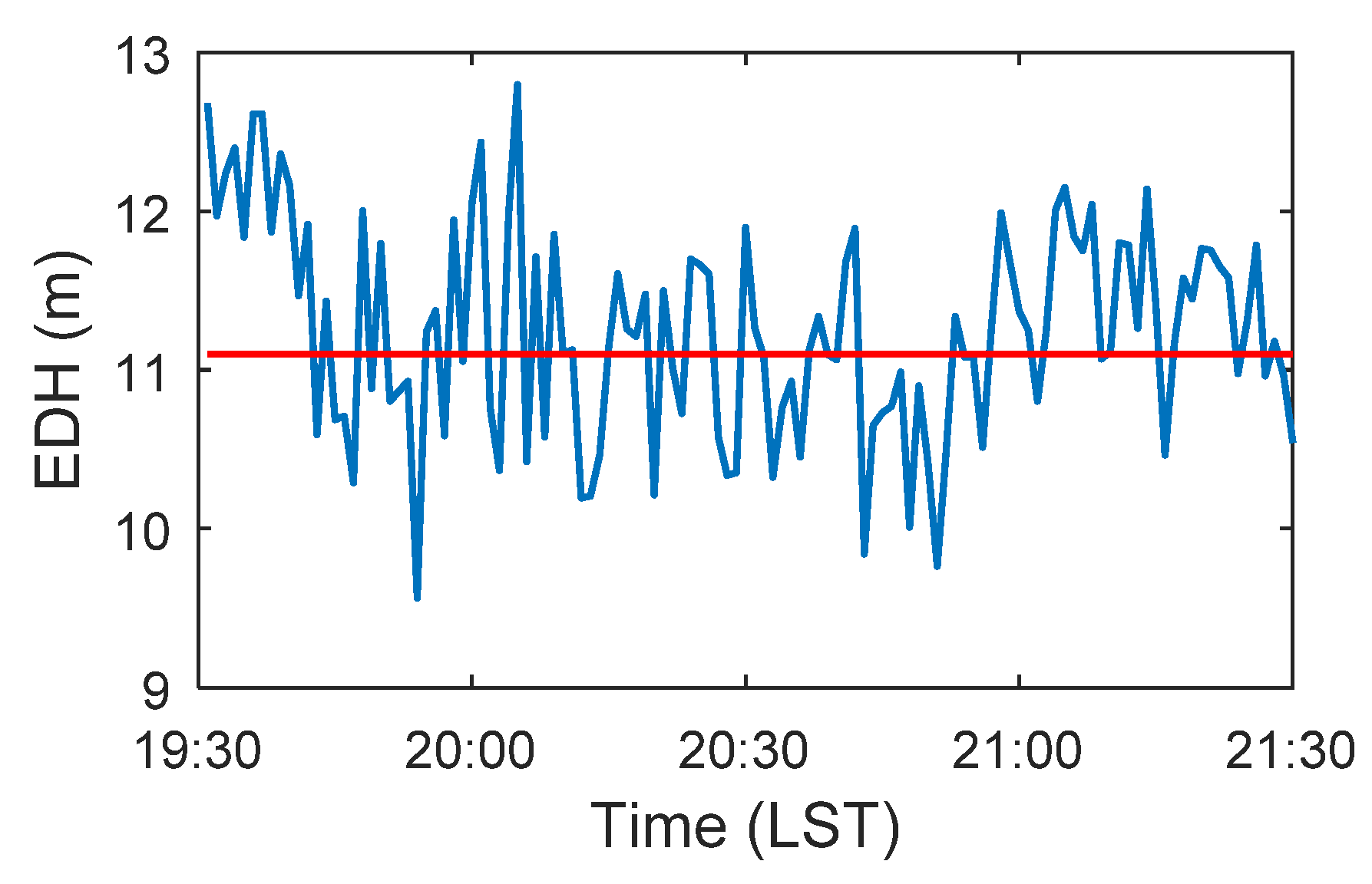
The variation of the EDH, from 19:30 LST on 5 September to 21:30 LST on 5 September 2017, is shown in Figure 4.

Figure 4 shows that the average EDH is ~11 m (red line). The minimum and maximum EDH are ~9.5 and ~13 m, respectively, and the variation range is ~3.5 m. The short-term variation of the EDH is mainly caused by the change of hydrometeorological parameters, systematic error of the sensor, and measurement error. Due to the non-stationary characteristics of the EDH, it is difficult to nowcast the EDH.

2.2. Deep Learning Network Selection

The nowcasting of the EDH is based on the data of the previous period and can be expressed by the following equation [19]:

$$y(t)=H(x(t),h(t-1)),$$

(4)

where $x(t)$ is the EDH measured at the current time, $h(t-1)$ is the historical characteristic EDH, $y(t)$ is the result of nowcasting, and $H$ is the nonlinear network model. Based on the choice of an appropriate deep learning network, the continuous time variation and non-stationary characteristics of the EDH can be determined.

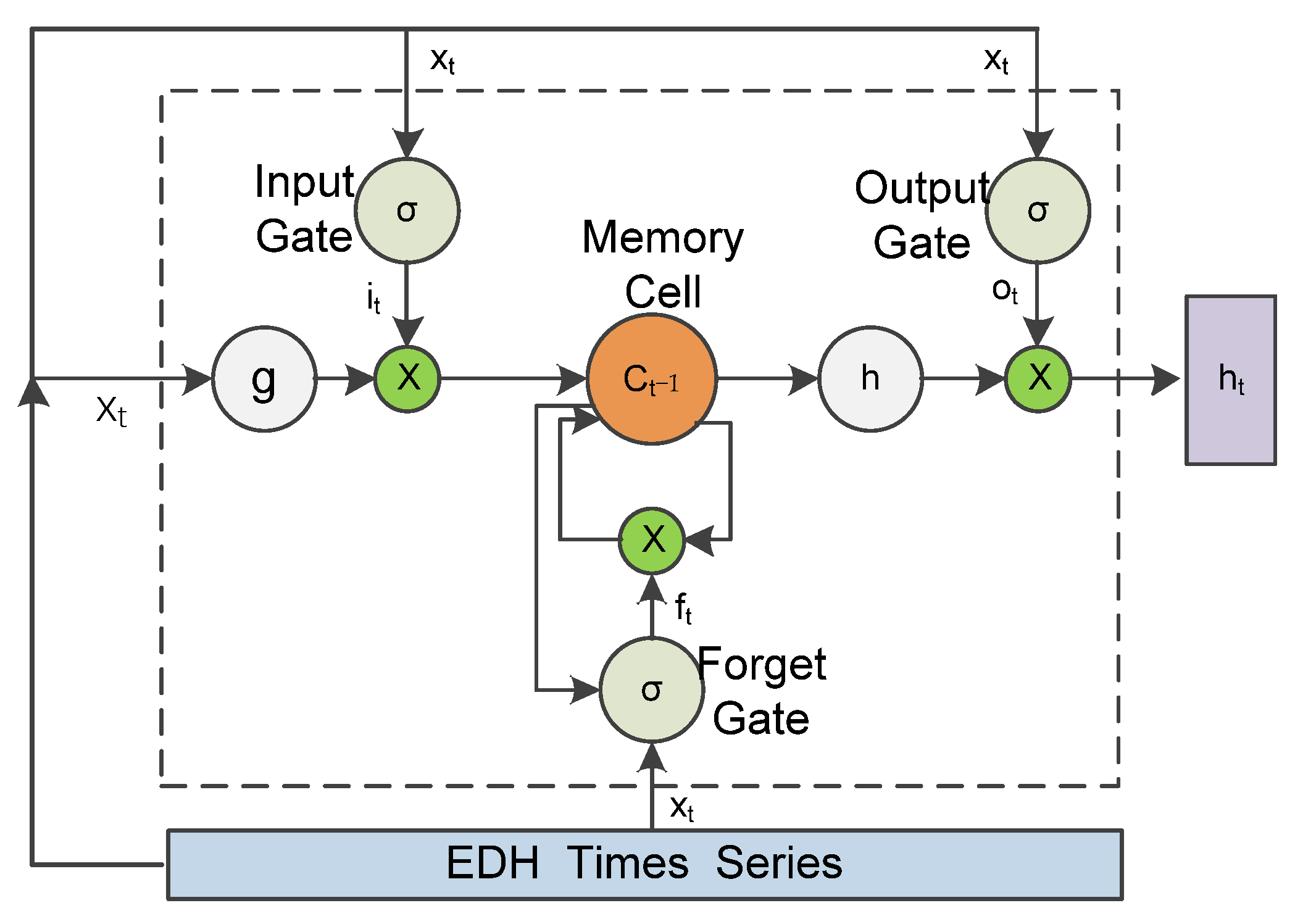
With the continuous development of deep learning technology, a variety of deep learning networks have been established in recent years. At present, deep neural networks (DNNs), recurrent neural networks (RNNs), and convolutional neural networks (CNNs) are commonly used. The RNN is one of the most effective networks for time series data processing. By introducing a cyclic structure, it can realize time series data analysis and prediction. However, the learning process of the RNN is characterized by gradient vanishing and explosion phenomena, which cannot evaluate long-term nonlinear relationships. To solve this problem, several researchers have proposed the use of an LSTM model. The LSTM, which is a special type of RNN, was proposed by Hochreiter et al. [20]. On the basis of a RNN, LSTM adds three gates—the input, output, and forget gates—based on which the gradient disappearance or gradient explosion of the RNN can be overcome. Therefore, the LSTM is suitable for the classification, processing, and prediction of time series. It is one of the most advanced architectures that can be used for the deep learning of time series [21,22]. Thus, the LSTM was selected to nowcast the EDH in this study. The structure of the LSTM memory unit is shown in Figure 5.

In the LSTM, $x_i$ is the EDH input at time t and $h_i$ is calculated with the following equations [23]:

$$i_t=\sigma (W_{ix}{x}_t+W_{ih}{h}_{t-1}+W_{ic}{c}_{t-1}+b_i)$$

(5)

$$i_t=\sigma (W_{ix}{x}_t+W_{ih}{h}_{t-1}+W_{ic}{c}_{t-1}+b_i)$$

(6)

$$o_t=\sigma (W_{ox}{x}_t+W_{oh}{h}_{t-1}+W_{oc}{c}_{t-1}+b_o)$$

(7)

$$c_t=f_t^0{c}_{t-1}+i_t^0\phi (W_{cx}{x}_t+W_{ch}{h}_{t-1}+b_c)$$

(8)

$$h_t=o_t^0\phi (c_t^{}),$$

(9)

where $i_t$, $f_t$, $o_t$, and $c_t$ are the outputs of the input gate, forget gate, memory cell, and output gate, respectively; $\sigma$ is a sigmoid function; and $g$ and $h$ are the activation functions from input to output of the memory cells, usually hyperbolic tangent functions tanh.

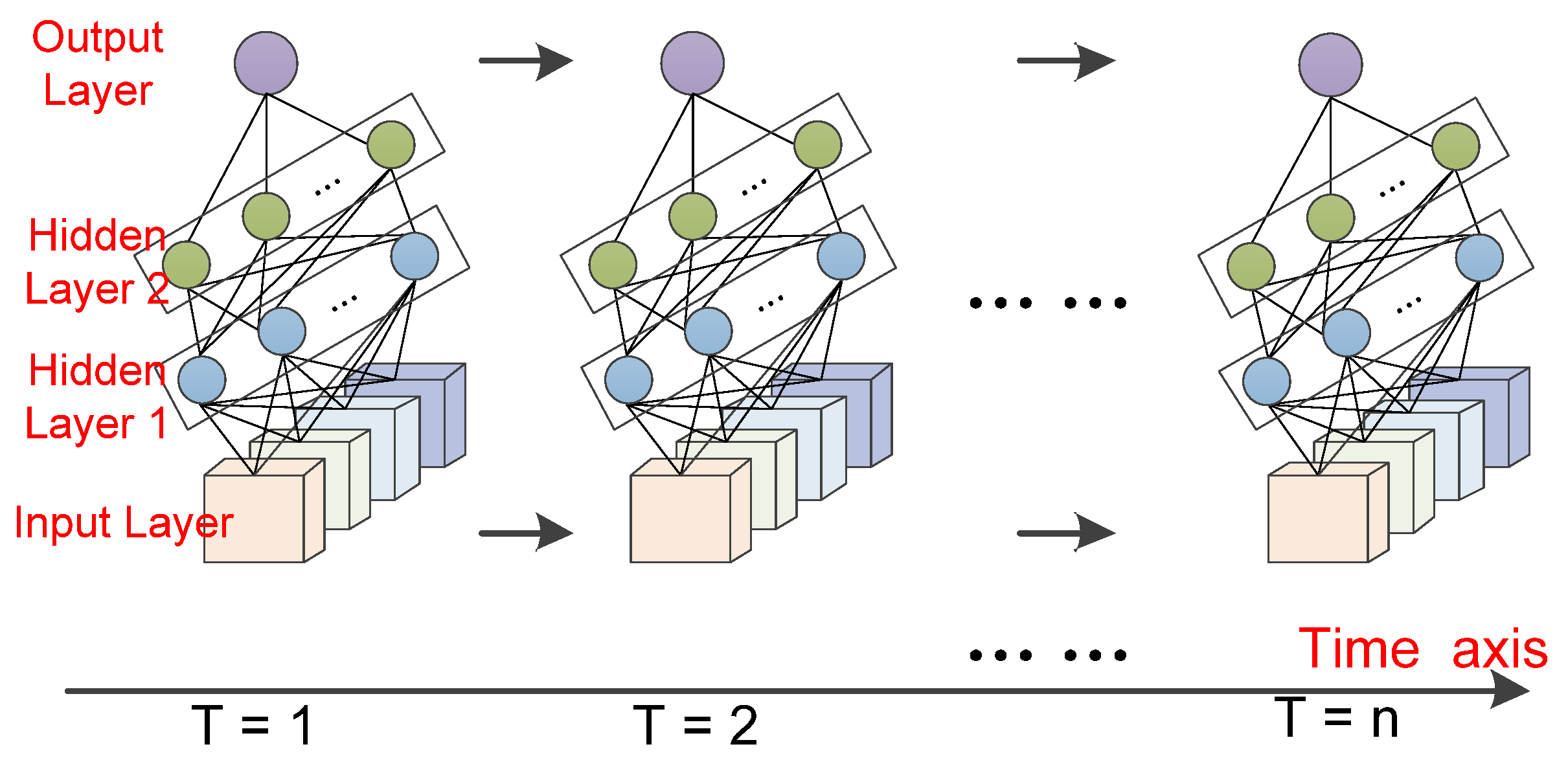
The EDH nowcasting framework based on the LSTM network is shown in Figure 6. The framework comprises three layers: input, hidden, and output layers. The input layer is the time series of the EDH, which is constructed by the measured EDH data; the hidden layer is composed of the LSTM layer and Dense layer; and the output layer is the EDH nowcasting result.

2.3. EDH Nowcast Model Based on the LSTM Network

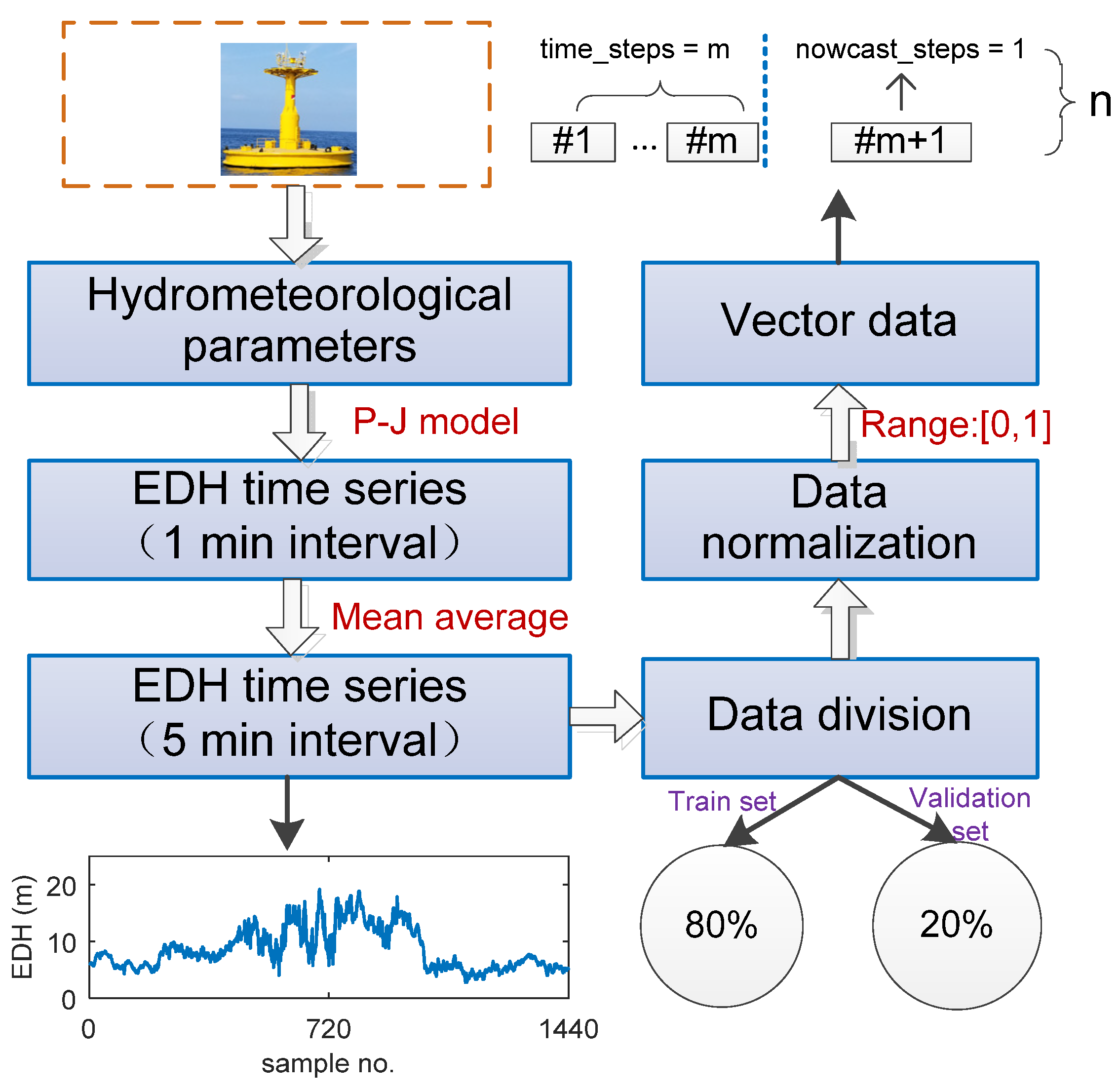
The EDH nowcast model based on the LSTM network is shown in Figure 7. First, a large amount of measured EDH data were used to build a training data set. Second, the nowcast model was established using the LSTM network, and the parameters were set.

2.3.1. Training Data Construction

The training data are the EDH data measured in Qingdao, Shandong, China, from July 2017 to March 2019, with a time resolution of 1 min and total number of samples of ~800,000. To reduce the influence of systematic and random errors and meet the format requirements for input data of the LSTM network, the original data must be processed. The processing flowchart is shown in Figure 8.

The EDH data processing comprises three steps:

• Step 1: Moving average

The real-time monitoring of the EDH data strongly fluctuates and cannot accurately reflect the real situation. Therefore, it is necessary to smooth the measured data. In this study, the moving average method was used for the monitoring data. After the data were averaged, the time resolution of the EDH data was 5 min and the total amount of samples was ~160,000.

• Step 2: Data division

After averaging, the EDH data were divided into training and test sets, accounting for 80% and 20% of the total data, respectively.

• Step 3: Data normalization

Data normalization was used to linearly transform the original data without affecting the data distribution or relationship between the data such that the resulting value is mapped between [0,1] or [−1,1]. Data normalization can accelerate the speed of the gradient descent; thus, the optimal solution can be identified and the prediction accuracy might be improved. In this paper, the training and test set data were mapped between [0,1].

2.3.2. Model Parameters

Model parameters, such as the optimization method, dropout rate, number of input and output layer nodes, number of hidden layers, number of hidden layer neurons, activation function, and loss function, play a vital role in the model performance. Some of the parameters were set when the model was built; the remaining parameters were first set to initial values and then optimized based on further analysis of the model performance. For the specific analysis, please see Section 4. The determined parameters are as follows:

• Number of epochs: The problem solved in this paper is similar to that in Zhao et al. [15] and the number of inputs is similar. Therefore, the number of epochs was set to 200, referring to the number used in Zhao et al. [15].
• Number of hidden layers: In this study, three hidden layers [12] were used including two LSTM layers and one fully connected layer (Dense).
• Number of neurons in the output layer: In this study, the future EDH is predicted; therefore, the number of neurons in the output layer is 1.
• Activation function: In the neural network, a functional relationship exists between the output of the upper node and input of the lower node. This function is called the activation function. Common activation functions are the Sigmoid, tanh, Rectified Linear Unit (ReLu), and linear functions. For the EDH nowcasting of this study, the ReLu and linear functions were used as activation functions [24].
• Loss function: The loss function guides the network parameter learning by calculating the error between the predicted and real samples such that the model reaches a convergence state. In this study, we used the mean_squared_error function, which can be expressed as follows:

  $$loss=\frac{{\displaystyle \sum _{i=1}^n{\left(pred\left(i\right)-y\left(i\right)\right)}^2}}{n},$$

  (10)

  where $pred\left(i\right)$ represents the nowcasting result of the EDH, $y\left(i\right)$ represents the expected value of the EDH sample, and n is the number of EDH time series selected for the training.

3. Results

Test Results and Analysis

To verify the superiority of the model proposed in this paper, the EDH nowcasting results were compared. In this paper, two representative time series data forecasting methods were selected: SVM and artificial neural network (ANN).

The SVM is an important data mining algorithm. It is a binary classification algorithm that supports linear and nonlinear classification [25]. It has been rapidly developed since the 1990s leading to the derivation of a series of improved and extended algorithms [26,27]. The EDH time series is defined as follows:

$$HS={\left\{Hi\right\}}_{i=1}^N,$$

(11)

where N is the length of the time series of the EDH. Support vector regression can be expressed as follows:

$$f(x)=w^T\varphi (x)+b,$$

(12)

where $\varphi$ is the input feature that maps the input vector $x$ to the high-dimensional space and $w$ $b$ are the model parameters to be estimated from the EDH.

The ANN, based on the principles of NNs in biology, is a mathematical model that simulates the processing of complex information by the nervous system of the human brain. Three ANN layers were used in this study and the ReLU and linear functions were utilized as activation functions for the hidden and output layers, respectively. EDH nowcasting can be expressed as follows:

$$f(x)=w_0^T(\mathrm{Re}LU(w_1^{T}x+b_1))+b_0,$$

(13)

where $x$ is the time series of the EDH; $w_1^T$ and $w_0^T$ are the weight matrix of the hidden and output layers, respectively; and $b_0$ and $b_1$ are the offsets of the hidden and output layers, respectively.

In this study, the mean absolute percentage error (MAPE), mean absolute error (MAE), and root mean square error (RMSE) were used to evaluate the accuracy of the forecast results. The formula of MAPE, MAE, and RMSE are as follows:

$$MAPE={\displaystyle {\sum }_{i=1}^n\left|\frac{{\widehat{h}}_i-h_i}{h_i}\right|}\times \frac{100\%}{n}$$

(14)

$$MAE=\frac{1}{n}\times {\displaystyle {\sum }_{i=1}^n\left|{\widehat{h}}_i-h_i\right|}$$

(15)

$$RMSE=\sqrt{\frac{1}{n}\times {\displaystyle {\sum }_{i=1}^n{({\widehat{h}}_i-h_i)}^2}},$$

(16)

where ${\widehat{h}}_i$ is the nowcast result, $h_i$ is the true value of the EDH, and n is the total number of samples.

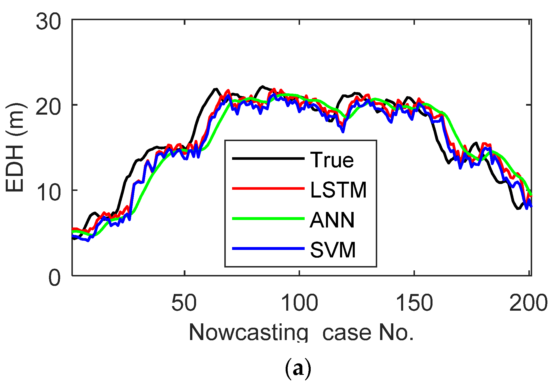
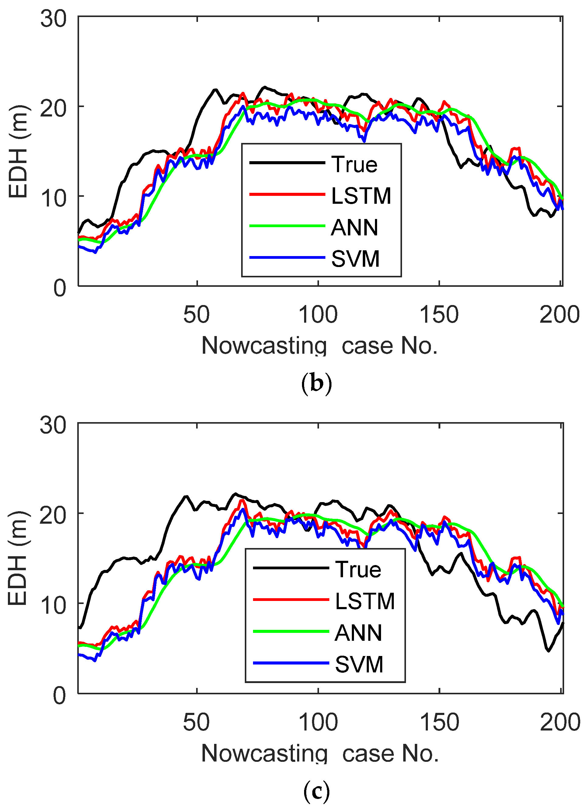
Figure 9 shows that the nowcast results of the three methods match the true EDH when the forecast duration is 30 min and the error is small; when the forecast duration is 60 or 120 min, the nowcast result error significantly increases. Among the three nowcasting methods, the LSTM yields the best nowcast results, which may be due to the fact that the LSTM uses more information about the EDH in the model building process.

To quantitatively describe the advantages of this method, ~38,000 sets of EDH data were used for the prediction and the RMSE, MAE, and MAPE of the LSTM, ANN, and SVM methods were calculated. The results are compared in

Table 2. Comparison of nowcast results based on different models.

Forecast Duration	LSTM			SVM			ANN
	RMSE	MAE	MAPE	RMSE	MAE	MAPE	RMSE	MAE	MAPE
30	1.28	0.81	10.41	1.37	0.95	13.16	1.61	1.02	13.72
60	1.89	1.18	14.88	1.92	1.28	17.08	2.16	1.38	17.43
120	2.68	1.74	21.90	2.84	1.85	23.31	2.85	1.87	23.19

.

Table 2 shows that the RMSE, MAE, and MAPE derived from the proposed model are smaller than those of the other two models. At a forecast time of 30 min, the advantage of the model proposed in this study is the most notable and the MAPE is better than that of the other two models (~3% smaller).

Table 2 and Figure 9 show that the proposed model has a higher accuracy and better applicability than the SVM and ANN methods with respect to the nowcasting of the EDH. The results also indicate the advantages of the use of the LSTM network for the time series prediction.

4. Effects of the Parameters on Nowcasting Accuracy

4.1. Effect of the Input Vector Dimension on Nowcasting Accuracy

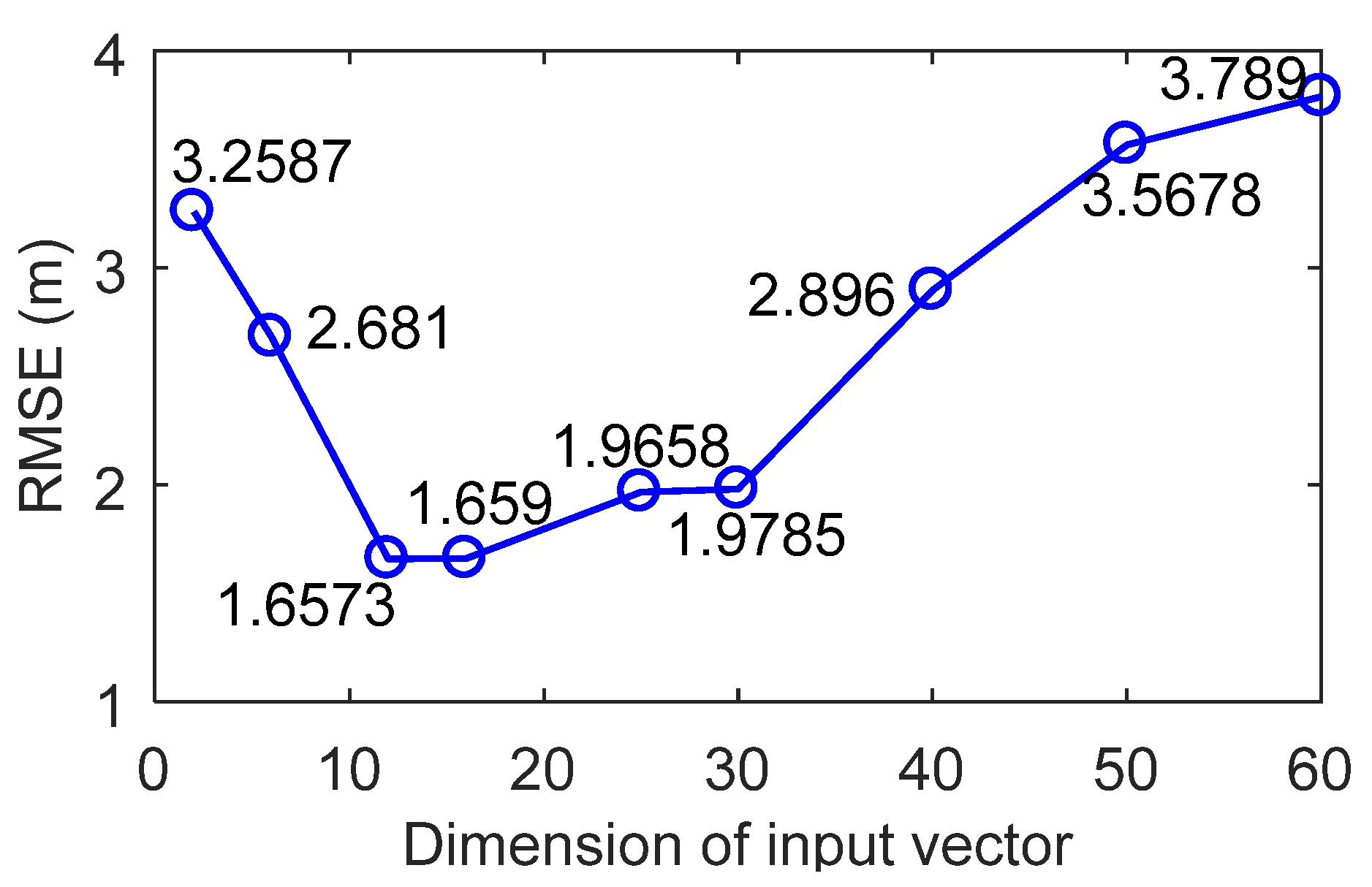
The input vector dimension refers to the amount of EDH data received by input layer neurons. If the amount of input EDH data is small, the change of the EDH cannot be determined; if the amount of input EDH data is large, the data farther away from the forecast time point may affect the nowcasting results, resulting in a lower nowcasting effect. EDH nowcasting accuracy changes with the input vector dimension, as shown in Figure 10. When the input vector dimension is small, the root mean squared error (RMSE) is large. As the dimension increases, the RMSE decreases; it is the smallest when the dimension is 12.

4.2. Effect of the Dropout Rate on Nowcasting Accuracy

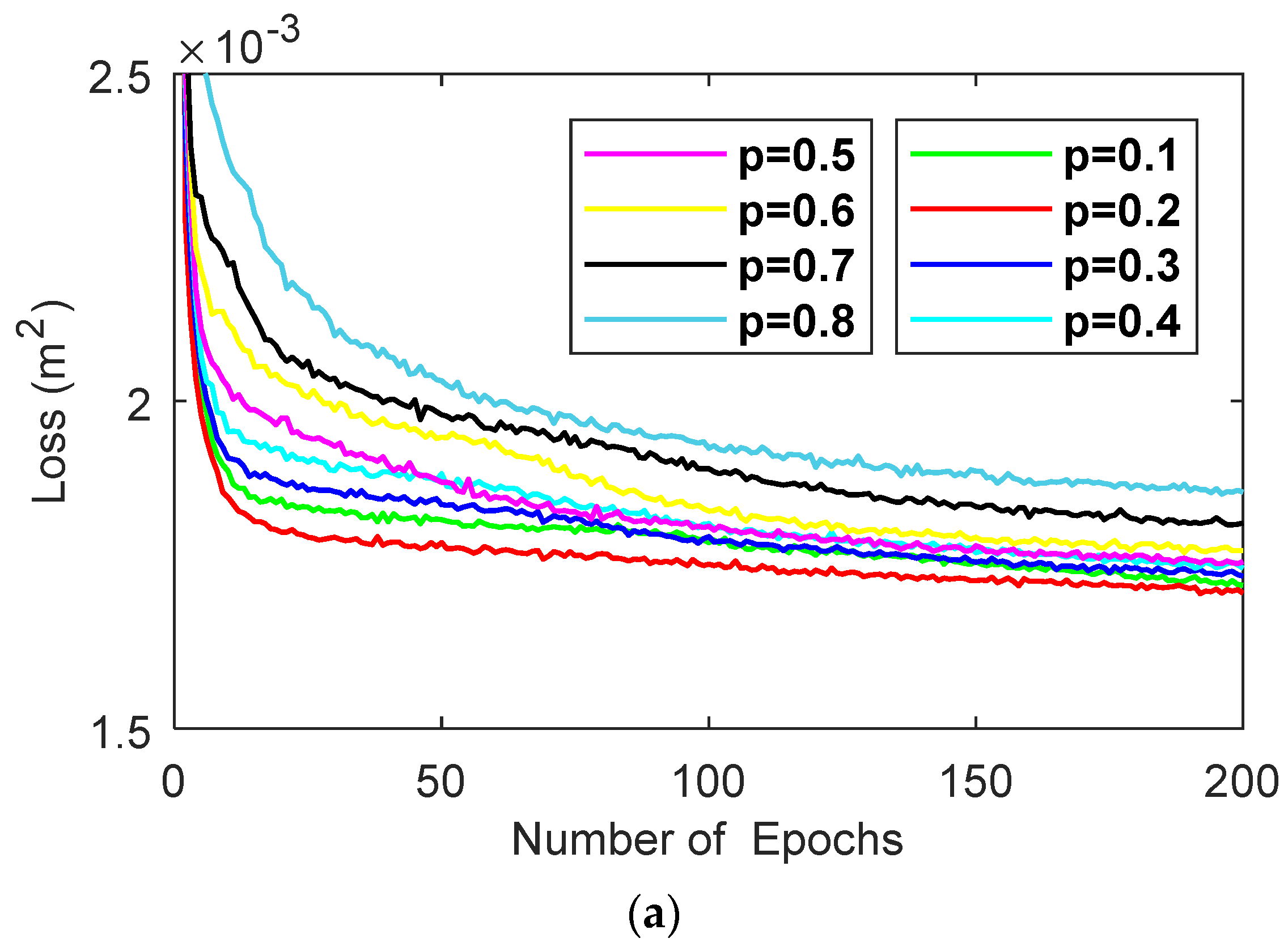
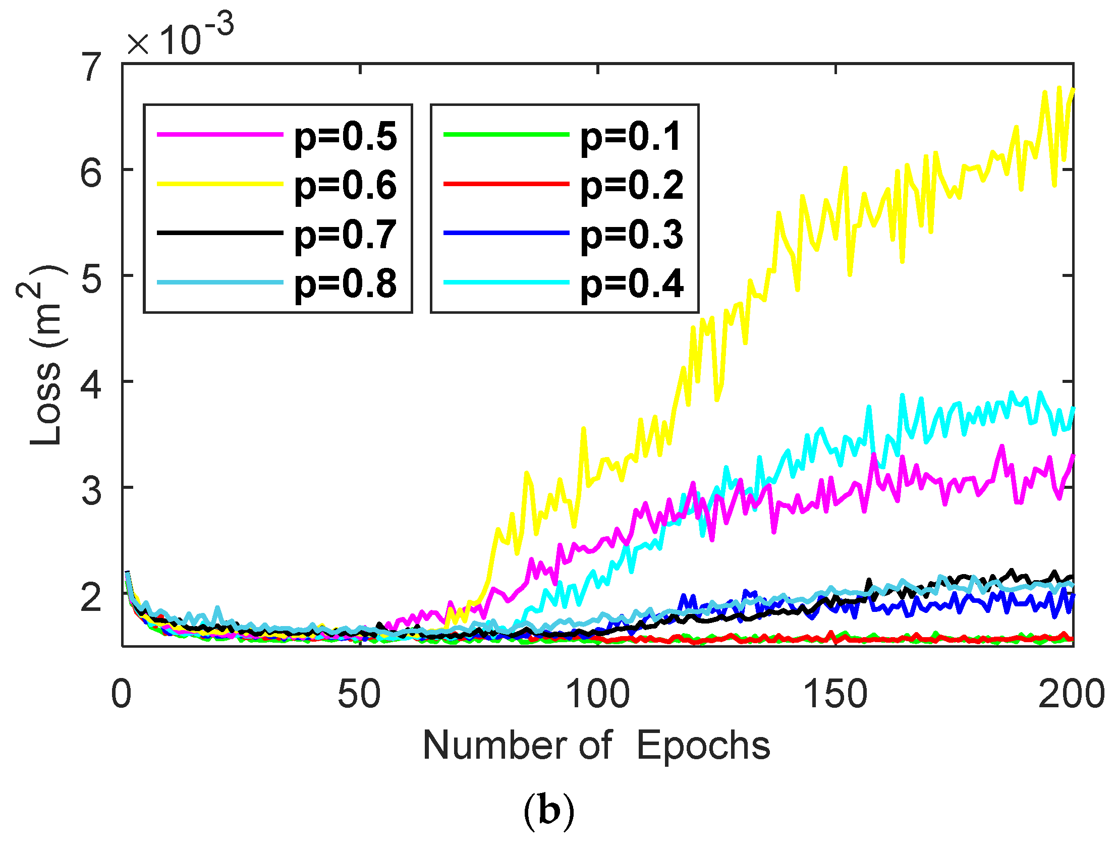
The dropout method was proposed by Hinton [10] and is one of the main methods used to prevent the overfitting of deep neural network models. During overfitting, the model obtains a small loss function for the training data and a large loss function for the test data. In the dropout method, the model randomly “drops” hidden layer neurons with the probability p during training, preventing the model from relying too heavily on local features and leading to a more generalized model. The interval of probability p is [0,1]. We selected p = 0.1, 0.2, 0.3, 0.4, 0.5, 0.6, 0.7, and 0.8 and analyzed the effect of the probability p on the model. Under different p-values, the loss function changes with the number of epochs, as shown in Figure 11.

Figure 11 shows that the training set error continues to decrease for p > 0.2. The validation set error first decreases and then increases, indicating that the model is overfitting and the model generalization ability is poor. When p = 0.2, the model training set and test set errors change relatively smoothly, no overfitting occurs, and the difference between the training set and test set errors is small.

The change in EDH nowcasting accuracy depending on different p-values used to build a 1 h nowcasting model is shown in Figure 12. When p = 0.2, nowcasting accuracy is highest.

4.3. Influence of the Number of Hidden Layer Neurons on Nowcasting Accuracy

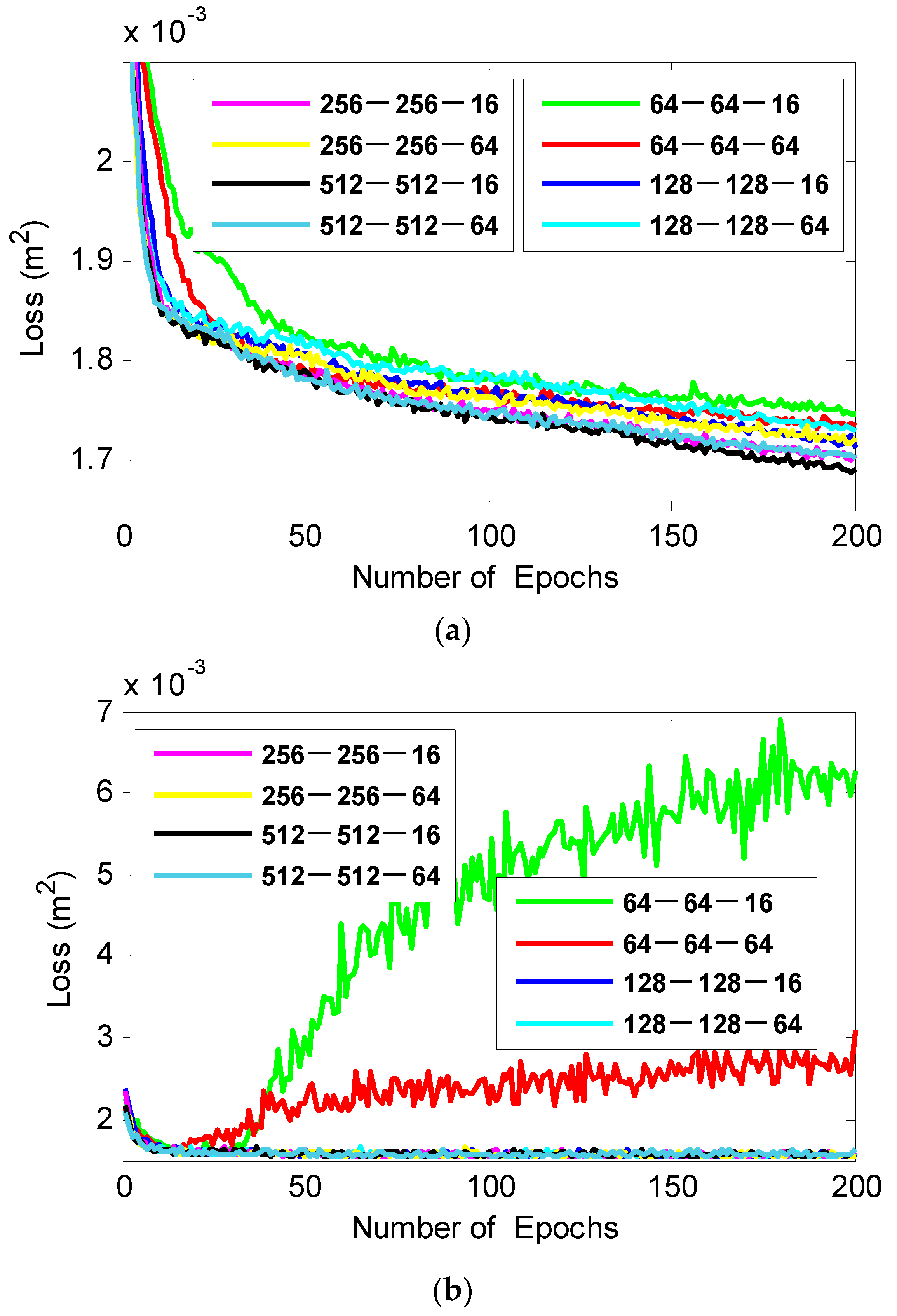
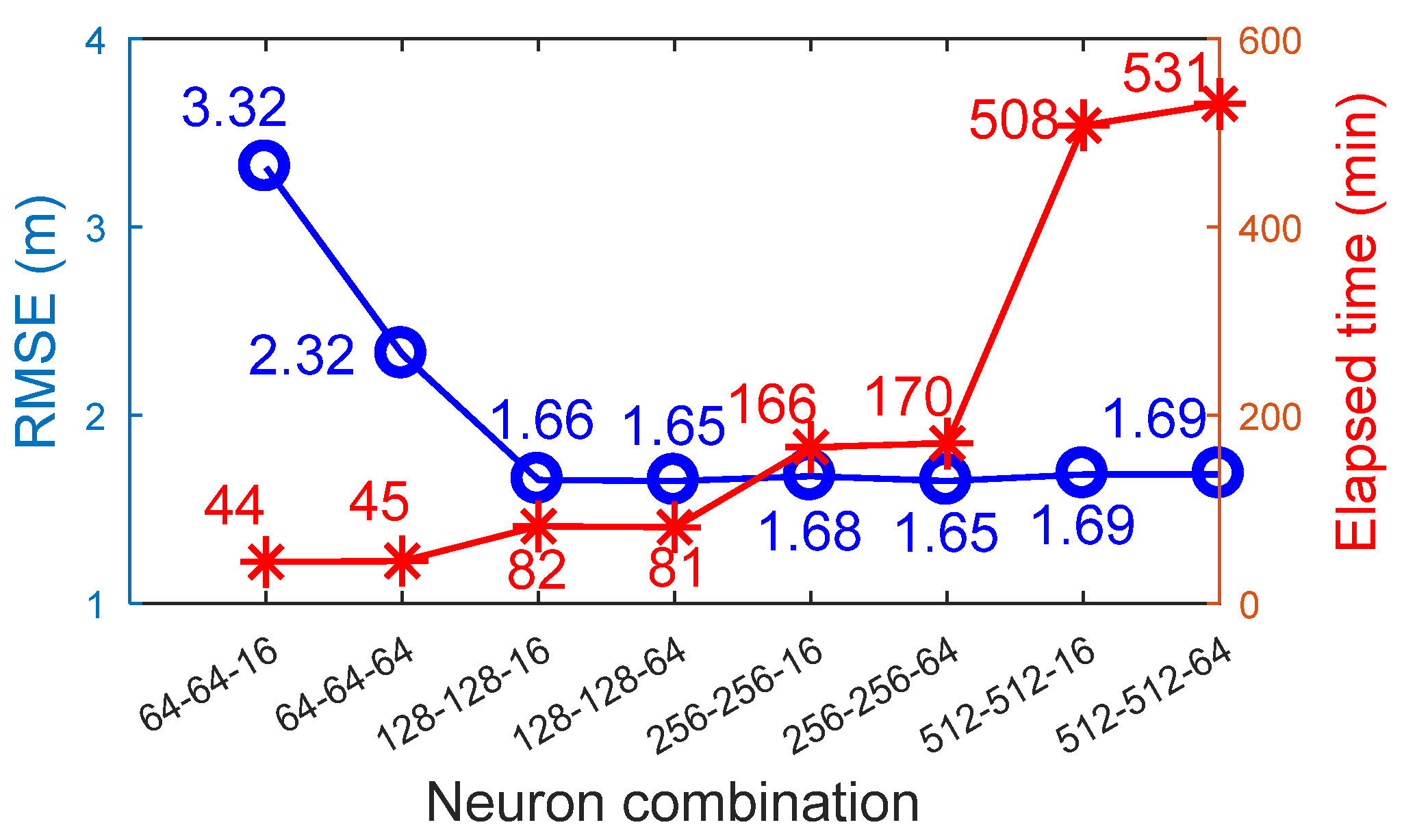
The number of neurons affects nowcasting accuracy and training time. A small number of hidden layer neurons will lead to an insufficient network performance; a large number of neurons leads to a good network performance but will increase network training time. In this study, the value range of the LSTM layer in the hidden layer is 64, 128, 256, and 512, and the numbers of fully connected layers are 16 and 64, a total of 8 combinations. The effect of different combinations on the model performance is shown in Figure 13.

Figure 13 shows that the error of the test set first decreases and then increases when the number of neurons in the LSTM layer is 64, indicating that the model is overfitting. The training set error, test set error, and time consumption corresponding to a number of neurons above 64 are shown in Figure 14.

Figure 14 shows that the difference in nowcasting accuracy under different neuron combinations is small when the number of neurons in the LSTM layer is greater than 64, indicating that an increase in the number of neurons does not significantly improve the nowcasting accuracy of the model but leads to an increased training time. Considering the nowcasting accuracy of the model and time consumption of the training, a combination of 128, 128, and 64 neurons were used for the model in this study.

In later research, more EDH data could be used for model training, and more parameter combination schemes should be compared and analyzed. The method described in this paper can be applied to the nowcasting of hydrometeorological parameters.

5. Conclusions

In this study, a nowcasting model for the EDH is proposed. Based on this model, the EDH parameters can be obtained 0–2 h in advance, providing environmental information to maximize the operational power of radar. First, an EDH nowcasting model was established based on the LSTM network. Second, the effects of different hyperparameters on the performance of the model were analyzed and a set of optimized parameters was identified. Finally, the proposed model was compared with traditional methods. The results of the comparison indicate that the model proposed in this study has better nowcasting accuracy. In future research, more data can be used for the model training to further optimize the model parameters and improve nowcasting accuracy.

References

1. Babin, S.M.; Young, G.S.; Carton, J.A. A new model of the oceanic evaporation duct. J. Appl. Meteorol. 1997, 36, 193–204. [Google Scholar] [CrossRef] [Green Version]
2. Liu, C.G. Research on evaporation duct propagation and its applications. D.E. Thesis, School of Electronic Engineering, Xidian University, Xi’an, China, 2003. [Google Scholar]
3. Ding, J.L. Contrast on occurrence of evaporation ducts in the South China. Chin. J. Radio Sci. 2009, 24, 1018–1023. [Google Scholar]
4. Poskitt, D.S.; Tremayne, A.R. The selection and use of linear and bilinear time series models. Int. J. Forecast. 1986, 2, 101–114. [Google Scholar] [CrossRef]
5. De Gooijer, J.G.; Hyndman, R.J. 25 years of time series forecasting. Int. J. Forecast. 2006, 22, 443–473. [Google Scholar] [CrossRef] [Green Version]
6. Xie, L. Research on clutter simulation and sea clutter prediction of broadband radar. J. Ambient Intell. Humaniz. Comput. 2019, 1–8. [Google Scholar]
7. Engle, R.F. Autoregressive conditional heteroscedasticity with estimates of the variance of united kingdom inflation. Econometrica 1982, 50, 987–1007. [Google Scholar] [CrossRef]
8. Alpaydin, E. Introduction to Machine Learning, 3rd ed.; The MIT Press: Cambridge, MA, USA, 2014. [Google Scholar]
9. Hastie, T.; Tibshirani, R.; Friedman, J. The Elements of Statistical Learning: Data Mining Inference and Prediction; Springer: Berlin/Heidelberg, Germany, 2009. [Google Scholar]
10. Krizhevsky, A.; Sutskever, I.; Hinton, G.E. ImageNet classification with deep convolutional neural networks. In Proceedings of the International Conference on Neural Information Processing Systems 2012, Lake Tahoe, CA, USA, 3–6 December 2012. [Google Scholar]
11. Doetsch, P.; Kozielski, M.; Ney, H. Fast and robust training of recurrent neural networks for offline handwriting recognition. In Proceedings of the 14th International Conference on Frontiers in Handwriting Recognition 2014, Hersonissos, Greece, 1–4 September 2014. [Google Scholar]
12. Guo, X.W.; Wu, J.J.; Zhang, J.P.; Han, J. Deep learning for solving inversion problem of atmospheric refractivity estimation. Sustain. Cities Soc. 2018, 43, 524–531. [Google Scholar] [CrossRef]
13. Paulus, R.A. Practical application of an evaporation duct model. Radio Sci. 1985, 20, 887–896. [Google Scholar] [CrossRef]
14. Zhu, X.Y.; Li, J.C.; Zhu, M.; Jiang, Z.H.; Li, Y.L. An evaporation duct height prediction method based on deep learning. IEEE Geosci. Remote Sens. Lett. 2018, 9, 1307–1311. [Google Scholar] [CrossRef]
15. Zhao, J.; Wu, J.J.; Guo, X.W.; Han, J.; Yang, K.; Wang, H.G. Prediction of radar sea clutter based on LSTM. J. Ambient Intell. Humaniz. Comput. 2019, 1–8. [Google Scholar] [CrossRef]
16. Babin, S.M. A new model of the oceanic evaporation duct and its comparison with current models. Master’s Thesis, University of Maryland, College Park, MD, USA, 1996. [Google Scholar]
17. Hitney, H.V.; Richter, J.H.; Schefer, M.H. Integrated Refractive Effects Prediction System 1978. U.S. Patent 4,125,893, 14 November 1978. [Google Scholar]
18. Patterson, W.L.; Hattan, C.P.; Lindem, G.E. Engineer’s Refractive Effects Prediction System (EREPS); Naval Command, Control and Ocean Surveillance Center: San Diego, CA, USA, 1994. [Google Scholar]
19. Ma, L.; Wu, J.; Zhang, J.; Wu, Z. Sea clutter amplitude prediction using a Long Short-Term Memory Neural Network. Remote Sens. 2019, 11, 2826. [Google Scholar] [CrossRef] [Green Version]
20. Hochreiter, S.; Schmidhuber, J. Long Short-Term Memory. Neural Comput. 1997, 9, 1735–1780. [Google Scholar] [CrossRef] [PubMed]
21. Hochreiter, S. Untersuchungen zu Dynamischen Neu-Ronalen Netzen. Master’s Thesis, Technische Universität München, München, Germany, 1991. [Google Scholar]
22. Bengio, Y.; Simard, P.; Frasconi, P. Learning long-term dependencies with gradient descent is difficult. IEEE Trans. Neural Netw. 1994, 5, 157–166. [Google Scholar] [CrossRef] [PubMed]
23. Gers, F.A.; Schmidhuber, J.; Cummins, F. Learning to Forget: Continual Prediction with LSTM. Neural Comput. 2000, 12, 2451–2471. [Google Scholar] [CrossRef] [PubMed]
24. LI, J.X. Tensor Flow Technology Analysis and Actual Combat; The People’s Posts and Telecommunications Press Publishers: Beijing, China, 2017. [Google Scholar]
25. Vapnik, V. Statistical Learning Theory; Elsevier B.V.: Amsterdam, The Netherlands, 1998; Volume 3, pp. 401–492. [Google Scholar]
26. Qin, J.; He, Z.S. A SVM face recognition method based on Gabor-featured key points. In Proceedings of the 2005 International Conference on Machine Learning and Cybernetics, Guangzhou, China, 18–21 August 2005; pp. 5144–5149. [Google Scholar]
27. Sun, A.; Lim, E.P.; Ng, W.K. Web classification using support vector machine. In Proceedings of the 4th International Workshop on Web Information and Data Management, McLean, VA, USA, 8 November 2002; pp. 96–99. [Google Scholar]
Short Biography of Author
Jie Han received a B.Sc degree from the China Research Institute of Radiowave Propagation, Qingdao, China, in 2008. He is currently pursuing a Ph.D. degree in signal and information processing from the School of Electronic Engineering, Xidian University, Xi’an, China. His research interests include atmospheric duct monitoring, atmospheric duct forecasting, and inversion algorithms. Jiaji Wu received a B.Sc degree in electrical engineering from Xidian University, Xi’an, China, in 1996, an M.Sc degree from the National Time Service Center, Chinese Academy of Sciences, in 2002, and a Ph.D. degree in electrical engineering from Xidian University in 2005. He is currently a professor with Xidian University. His current research interests include image processing, still image coding, hyperspectral/multispectral image compression, communication, and high-performance computing.
Figure 1. Radar detection system.
Remotesensing 13 01577 g001
Figure 2. Geographical location of the offshore buoy and sensor location.
Remotesensing 13 01577 g002
Figure 3. Daily variation of the evaporation duct height (red line indicates the average EDH).
Remotesensing 13 01577 g003
Figure 4. Short-term variation of the EDH (red line indicates the average EDH).
Remotesensing 13 01577 g004
Figure 5. Structure of the LSTM memory unit.
Remotesensing 13 01577 g005
Figure 6. EDH nowcasting framework based on the LSTM network.
Remotesensing 13 01577 g006
Figure 7. EDH nowcast model.
Remotesensing 13 01577 g007
Figure 8. EDH data processing flow-chart.
Remotesensing 13 01577 g008
Figure 9. Comparison of the nowcasted evaporation duct heights. (a) 30-min forecast; (b) 60-min forecast; (c) 120-min forecast.
Remotesensing 13 01577 g009aRemotesensing 13 01577 g009b
Figure 10. Changes in nowcasting accuracy depending on the input vector dimension.
Remotesensing 13 01577 g010
Figure 11. Training error variations under different p−values depending on the number of epochs. (a) Variation of the training set error depending on the number of epochs (b) Variation of the test set error depending on the number of epochs.
Remotesensing 13 01577 g011aRemotesensing 13 01577 g011b
Figure 12. Nowcasting accuracy including p-values.
Remotesensing 13 01577 g012
Figure 13. Variation of the training error of different neuron combinations depending on the number of epochs. (a) Variation of the training set error depending on the number of epochs (b) Variation of the test set error depending on the number of epochs.
Remotesensing 13 01577 g013
Figure 14. Variation of the training error and elapsed time for different neuron number combinations. The blue and green lines represent the change of the RMSE and elapsed time, respectively.
Remotesensing 13 01577 g014