Article

Topside Ionosphere and Plasmasphere Modelling Using GNSS Radio Occultation and POD Data

by
Fabricio S. Prol
*,† and
M. Mainul Hoque
German Aerospace Center (DLR), Institute for Solar-Terrestrial Physics, Kalkhorstweg 53, 17235 Neustrelitz, Germany
*
Author to whom correspondence should be addressed.
These authors contributed equally to this work.
Remote Sens. 2021, 13(8), 1559; https://doi.org/10.3390/rs13081559
Submission received: 12 March 2021 / Revised: 13 April 2021 / Accepted: 15 April 2021 / Published: 17 April 2021
(This article belongs to the Section Atmospheric Remote Sensing)

Abstract

:
A 3D-model approach has been developed to describe the electron density of the topside ionosphere and plasmasphere based on Global Navigation Satellite System (GNSS) measurements onboard low Earth orbit satellites. Electron density profiles derived from ionospheric Radio Occultation (RO) data are extrapolated to the upper ionosphere and plasmasphere based on a linear Vary-Chap function and Total Electron Content (TEC) measurements. A final update is then obtained by applying tomographic algorithms to the slant TEC measurements. Since the background specification is created with RO data, the proposed approach does not require using any external ionospheric/plasmaspheric model to adapt to the most recent data distributions. We assessed the model accuracy in 2013 and 2018 using independent TEC data, in situ electron density measurements, and ionosondes. A systematic better specification was obtained in comparison to NeQuick, with improvements around 15% in terms of electron density at 800 km, 26% at the top-most region (above 10,000 km) and 26% to 55% in terms of TEC, depending on the solar activity level. Our investigation shows that the developed model follows a known variation of electron density with respect to geographic/geomagnetic latitude, altitude, solar activity level, season, and local time, revealing the approach as a practical and useful tool for describing topside ionosphere and plasmasphere using satellite-based GNSS data.

1. Introduction

Ionospheric measurements from Global Navigation Satellite System (GNSS) receivers onboard low Earth orbit (LEO) satellites are an outstanding data source to explore the plasmasphere and the ionosphere. GNSS signals transmitted in at least two frequencies can be used to compute electron density (Ne) profiles up to the LEO satellite height and Total Electron Content (TEC) values above the receiver altitude up to the GNSS satellite. However, the assimilation of Ne profiles and TEC values into a unique solution has continued to be a relevant challenge to any ionospheric/plasmaspheric system.
Empirical models such as NeQuick [1] and the International Reference Ionosphere extended to Plasmasphere (IRI-Plas) [2] are often used to describe the electron density profiles from 60 km up to the GNSS orbit altitude around 20,000 km. Both models are well known to provide good specifications of the general patterns of the ionosphere and plasmasphere [3]. However, as pointed out by Cherniak and Zakharenkova [4], IRI-Plas and NeQuick need to be essentially improved above the F2 layer peak (hmF2) for a better characterization of the topside TEC. Gulyaeva [5], for instance, has upgraded the IRI-Plas model using ground-based TEC observations from Global Ionospheric Maps (GIMs), but this approach deals with the difficulties of separating the bottomside TEC contribution from the topside TEC. This makes the use of satellite-based TEC to estimate electron density distributions a highly appealing option, since it already excludes the ionospheric contribution below the LEO height.
Among the methods using satellite-based GNSS observations to estimate electron density distributions, Prol et al. [6], Li et al. [7], Wu et al. [8], and others, revealed the GNSS Radio Occultation (RO) technique as a powerful tool to describe global features of the ionosphere from hmF2 up to 800 km. Additionally, Heise et al. [9] and Spencer and Mitchell [10] succeeded in applying tomographic solutions to estimate electron density profiles from LEO heights up to 20,000 km using TEC measurements. Wu et al. [11] have even assimilated satellite-based TEC measurements into the global core plasma model (GCPM) [12] using a 3DVar approach. However, all of these methods have used RO electron density and satellite-based GNSS-TEC as independent sources, i.e., they either use topside data or RO data. In the present work, we propose a method where LEO-based TEC measurements are used together with RO electron density profiles. We therefore take full advantage of the satellite-based GNSS observations to characterize the electron density from hmF2 up to 20,000 km.
The innovative approach of the proposed method uses the RO-Ne to create a background specification and assimilates the LEO-based TEC data into background electron density. Thus, we can avoid using any traditional ionosphere model (e.g., NeQuick, IRI) as a background. This approach takes advantage of the availability of numerous medium Earth orbit (MEO) satellites deployed by Global Positioning System (GPS) whose signals are being tracked by many LEO satellites for the continuous monitoring of the Earth’s ionosphere. For instance, the constellation of Formosa Satellite-7/Constellation Observing System for Meteorology Ionosphere and Climate (FORMOSAT-7/COSMIC-2) was recently launched with six satellites [13]. The Spire Global, Inc. [14] is continuously increasing the number of LEO satellites that can be used to retrieve RO electron densities and TEC measurements. The developed method will therefore benefit from future better data coverage. Given such interests, this work was carried out, where Section 2 shows the dataset used, Section 3 presents the mathematical formulation, Section 4 shows the experimental results, and Section 5 presents the conclusions.

2. Dataset

The method developed in this study is based on measurements collected by the Formosa Satellite Mission 3/Constellation Observing System for Meteorology, Ionosphere, and Climate (FORMOSAT-3/COSMIC, or just COSMIC). COSMIC satellite data are processed by the University Corporation for Atmospheric Research (UCAR) and obtained through the COSMIC Data Analysis and Archive Center (CDAAC) via the portal https://cdaac-www.cosmic.ucar.edu/ (accessed on 10 March 2021). We have used a level 1 product, namely podTec [15], which is derived from dual-frequency GPS measurements originally recorded for precise orbit determination (POD). Ray paths with an elevation angle lower than 20° or with negative TEC values are filtered out in preprocessing steps. Additionally, data from occultation retrieval of electron density profiles obtained in a level 2 processing step were used. An algorithm was applied to filter out electron density profiles with negative Ne values, peak height (hmF2) lower than 180 km or higher than 700 km and high electron density values, such as the electron density at the peak (NmF2) higher than 8 × 10 12 el/m 3 .
A period of six years was chosen to perform the analysis. Four years in distinct solar conditions were used as the basis for the model construction. The years 2008 and 2017 are attributed to low solar activity level, while 2012 and 2014 to high solar activity level. The model was validated using the data from 2013 and 2018 corresponding to high and low solar activity levels, respectively. Note that, during 2018, only a reduced number of COSMIC satellites (C001 and C006) was operational. The performance assessment was carried out based on ionosonde measurements of the Global Ionosphere Radio Observatory (GIRO) network [16], in situ electron density measurements of the Defense Meteorological Satellite Program (DMSP) [17], electron density values from the Van Allen Probes and TEC observations of the Meteorological Operational satellite A (METOP-A) satellite. NeQuick results are also used in the assessment of the model performance. The Fortran source code with default parameters was used to validate the NeQuick model in a climatological manner.
The used GIRO datasets are automatically scaled and downloaded from the portal http://giro.uml.edu/didbase/scaled.php (accessed on 10 March 2021). We have adopted the automatically scaled data ignoring values with the Confidence Score (C-Score) equal to zero or unknown precision −1. The used DMSP electron density data are processed by the Center for Space Sciences at the University of Texas (Dallas) and obtained through the Madrigal portal http://cedar.openmadrigal.org/ (accessed on 10 March 2021). The Van Allen Probes electron density data are processed by Zhelavskaya et al. [18] using the algorithm NURD (Neural-network-based Upper hybrid Resonance Determination). The NURD dataset is available at ftp://rbm.epss.ucla.edu/ftpdisk1/NURD (accessed on 10 March 2021), and we have selected the instruments Radiation Belt Storm Probes—A (RBSP-A) and RBSP-B for the evaluation. The used METOP-A data are processed by UCAR and downloaded through the CDAAC archive. All magnetic latitudes in this work were computed based on the International Geomagnetic Reference Field (IGRF), available at https://www.ngdc.noaa.gov/IAGA/vmod/igrf.html (accessed on 10 March 2021).

3. Method

The proposed approach has three major steps: (1) climatological modeling; (2) background construction and (3) tomographic reconstruction.

3.1. Climatological Modeling

The climatological modeling step is performed in order to derive average electron density profiles of the upper ionosphere and plasmasphere. We have modeled four ionospheric key parameters, namely the peak electron density NmF2, corresponding height hmF2, atmospheric scale height Hs and rate of change of scale height with respect to altitude d H s / d h . The peak values hmF2 and NmF2 are obtained directly from the RO profiles, while Hs and d H s / d h are obtained using the method shown in Prol et al. [19]. In such method, an approximated value of the scale height for each profile is updated using an iterative process that cycles through all electron density measurements until the maximum electron density error of the profile attains 10 4 electrons/m 3 . A linear fitting of the scale height is then performed to estimate Hs and d H s / d h values.
The electron density distribution from hmF2 up to 800 km height is modeled using four key parameters derived from RO observation. Above 800 km, POD TEC measurements are used to describe the general variability of the electron content. In this regard, slant TEC (STEC) measurements are converted to the vertical TEC (VTEC) using the mapping function shown by Foelsche and Kirchengast [20] with a single-shell height of 1300 km, since this single-shell height has presented one of the best performances in recent studies for satellite-based TEC [21]. A spherical harmonic function is then used to describe each parameter in time and space given by the following equation:
f ( ϕ m , t L ) = F 10 n = 0 N m = 0 n P n m sin ( ϕ m ) [ a n m cos ( π m t L 12 ) + b n m sin ( π m t L 12 ) ] + sin ( d o y ) F 10 n = 0 N m = 0 n P n m sin ( ϕ m ) [ c n m cos ( π m t L 12 ) + d n m sin ( π m t L 12 ) ] + cos ( d o y ) F 10 n = 0 N m = 0 n P n m sin ( ϕ m ) [ e n m cos ( π m t L 12 ) + f n m sin ( π m t L 12 ) ]
where f ( ϕ m , t L ) stands for the observations of any of the target parameters (NmF2, hmF2, Hs, d H s / d h and VTEC), ϕ m is the magnetic latitude, t L is the local time, P n m is the normalized associated Legendre polynomial, and a n m , b n m , c n m , d n m , e n m , f n m , are the coefficients to be determined in a least square adjustment with the degree N = 10. We have empirically checked that the degree N = 10 is enough to cover the data gaps when there are very few observations, such as in 2018 when a reduced number of COSMIC satellites was operational. The quantity F10 refers to the solar radio flux at 10.7 cm (F10.7 index) in solar flux units (sfu), which is smoothed applying a 365-day running average. The symbol doy refers to the day of the year converted to radian values (e.g., 2 π for the last day of the year plus one day).
The coefficients related to NmF2, hmF2, Hs and dHs/dh values are estimated using RO-Ne observations and coefficients related to VTEC values are estimated using POD TEC data. Data from 2008, 2012, 2014 and 2017 were used as the base for the model construction in order to capture electron density for both high and low solar activity. All data of two years (2008 and 2014) are used to estimate the coefficients af. In addition, data from 365 days prior to the date of interest are included to capture the most recent variabilities. This way, our solution adapts to the most recent solar activity given by the last one year of F10 values.
As shown in Equation (1), the model is dependent on the F10.7 index. We have adopted the 365 running mean since we apply a daily correction to the obtained coefficients. Indeed, there are some obvious inconsistencies in the correlation between the F10.7 index and the actual electron density, since the F10.7 index provides a measure of the solar irradiation while the electron density also depends on other geophysical indicators, such as location, local time, seasons, geomagnetic field configurations and atmospheric dynamics. Considering this, after estimating the coefficients to describe the spatial and time variation, we update the model based on daily observations. The output parameter is therefore the value obtained in Equation (1) multiplied by a ratio term computed in the day of interest.
The target parameter multiplied by the daily ratio term is given by Equation (2):
f e s t ( ϕ m , t L ) = < o b s > < f ( ϕ m o b s , t L o b s ) > f ( ϕ m , t L )
where o b s stands for the observations, i.e., the values measured by the RO inversion technique (NmF2, hmF2, Hs and dHs/dh) or by the POD instruments (VTEC), < o b s > is the average of all observations used in the day of interest, f ( ϕ m , t L ) is the value obtained by Equation (1), f e s t ( ϕ m , t L ) is the parameter corrected by the daily observations and < f ( ϕ m o b s , t L o b s ) > is the average of all estimated values with Equation (1) for all latitudes and times of the observations.
The purpose of Equation (2) is to apply a daily correction to the key parameters f ( ϕ m , t L ) estimated by Equation (1). This improves the solution of Equation (1) since the F10.7 index does not represent the daily state of the ionosphere. Indeed, after estimating the coefficients af, it is possible to describe climatological patterns of the ionosphere, but there is still some room for improvement to provide daily states. Similar approaches have been conducted to improve the IRI model by adapting the R12 and IG12 parameters to provide improved daily representations [22].

3.2. Background Construction

The background was defined in order to fill in each cell of a 3D grid with an initial electron density. After knowing the coefficients of Equation (1) and the daily ratio term of Equation (2), the 3D grid is built as a function of Local Time (LT), magnetic latitude, and altitude, with a resolution of 0.4 h, 2°, and 20 km, respectively. The altitude coverage refers up to 20,000 km. The background electron density between the hmF2 height and 800 km (i.e., LEO orbit height) is modeled using a Vary-Chap function together with parameters estimated in the climatological modeling step. Olivares-Pulido et al. [23] found that a linear Vary-Chap function is a good way to describe topside RO measurements above the hmF2 height. Therefore, the background electron density between the hmF2 height and 800 km is computed with the following linear Vary-Chap function:
N e = N m F 2 exp 0.5 ( 1 z exp z )
with:
z = h h m F 2 H s + d H s / d h ( h h m F 2 )
where all parameters (hmF2, NmF2, Hs, d H s / d h ) are derived from the developed climatological model (Equation (2)).
Above the altitude of 800 km, an extrapolation procedure is adopted. The extrapolation was conducted through a linear interpolation of the log(Ne) between 800 km and the plasmapause. In this work, the plasmapause location ( h p p ) is defined as the L-shell number 4 in the equatorial plane. We have defined such a location based on the works of Zhelavskaya et al. [18,24]. This simplified assumption is consistent with the cases of study in this work since they are related to quite time conditions. However, in case of a disturbed geomagnetic condition, a more appropriate L-shell number should be defined.
For a given profile, the electron density at h p p is defined as 4 × 10 8 el/m 3 . This value was defined based on the results obtained by [18]. Zhelavskaya et al. [18] have observed a trough-like pattern subtly decreasing electron density in the surroundings of the plasmapause. The plasmasphere magnitudes around the plasmapause are given as 2.6 in terms of log10 (Ne)cm 3 , which corresponds to 4 × 10 8 el/m 3 .
The interpolation between 800 km and h p p is then given for each latitude and LT of the 3D grid by the following equation:
N e = exp ( a + b h ) 1 / c
where a and b stand for the coefficients of the linear interpolation, and the term c represents a constant that controls how much the log ( N e ) differs from the linear pattern. This term c is estimated iteratively by running the linear least squares varying c from −40 to 40 with a step size of 0.05. The chosen c is the one that provides the closest VTEC value to the VTEC given by the climatological model. As a result, the final profile will provide a linear decrease of the l o g ( N e ) with increasing altitude adapted to follow the VTEC values of the climatological model.

3.3. Tomographic Reconstruction

In the tomographic reconstruction, STEC measurements from COSMIC collected during the dates of interest are used to update the electron density distribution of the background. The solutions are provided in a daily 3D grid distributed along LT, magnetic latitude and altitude with the same resolution of the background. The Algebraic Reconstruction Technique (ART) [25] is implemented as a basis of the developed tomography in order to provide fast inversions of STEC into electron densities. A first initial guess of electron density ( x j k ) at iteration k = 1 is derived from the background. ART then iteratively updates the electron density in each cell based on the difference between the TEC observations (y) and background STEC values ( j N A i j x j k ). The general ART is formulated as:
x j k + 1 = x j k + γ y i j = 1 N A i j x j k j = 1 N A i j 2 A i j
where γ is a relaxing parameter, y i is the ith STEC observation, A i j stands for the path lengths inside the boundaries of the voxel j and signal i, x j 0 is the electron density given by the background, and x j k is the electron density at iteration k obtained after each update.
In the traditional ART, the unknown x j k + 1 is updated at every instance. However, this approach is affected by the way the observation vector is sorted [26]. To overcome this problem, this work utilized the Simultaneous Iterative Reconstruction Technique (SIRT) [27], where the final reconstruction is obtained by taking the average correction after the differences ( y i j = 1 N A i j x j k ) of all i signals have been computed.
Typically, the relaxing parameter γ is a constant value. However, in order to better stabilize the ill-conditioned solution, we have defined the relaxing parameter with a significant dependence on the background. The adopted relaxing parameter is the same used by Prol et al. [28]:
γ = 0.2 ( x j 0 / x m a x 0 )
in order to keep the profile shape of the final iteration with similar patterns of the background, mainly when the electron density x j 0 is small.
The background updates are performed in the illuminated voxels. This may produce discontinuities in the final reconstructions due to data gaps. In the case of voxels where no rays pass through, two Gaussian functions are used to determine the amount of influence by the nearby voxels, similarly to Prol et al. [28]. The Gaussian half widths are taken as σ = 2.5° along the latitudes and longitudes (converted to local time). These half widths are defined with almost the same size of the voxels to mainly update the variations with the closest illuminated voxels.

4. Results

For practical reason, the results of the developed method will be referred to as results of tomography, since this was the last step of the developed method. However, it is important to mention that STEC measurements are obtained above the LEO satellite. Therefore, below the LEO satellite, results are mainly controlled by the climatological step. In case of the accuracy evaluation, NeQuick results are being compared with the assimilative approach. NeQuick is a climatological model, while our approach uses actual data. Therefore, it is expected to obtain similar or better results with the developed approach.

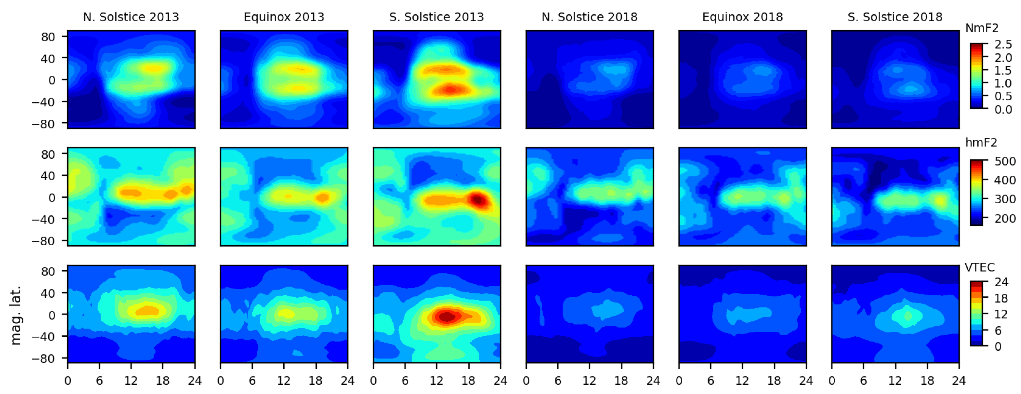
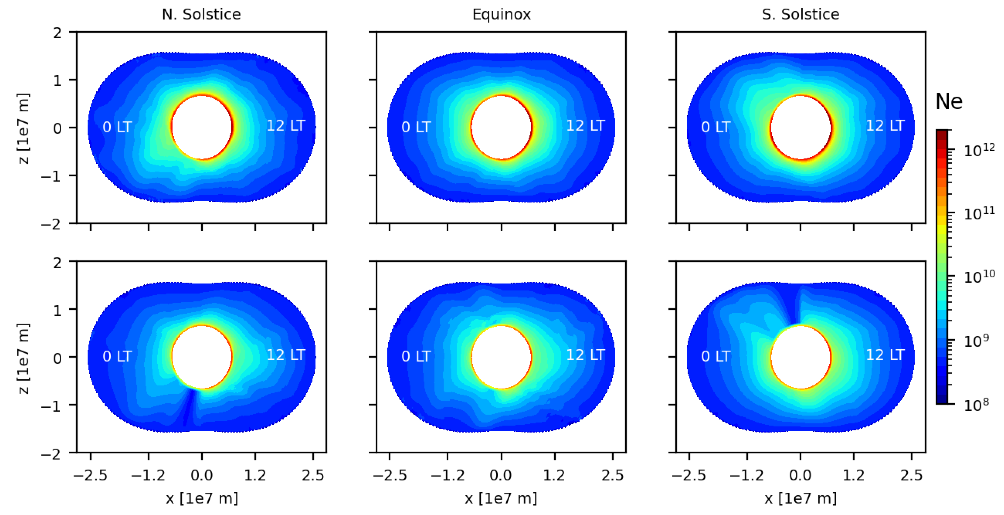
4.1. General Distributions
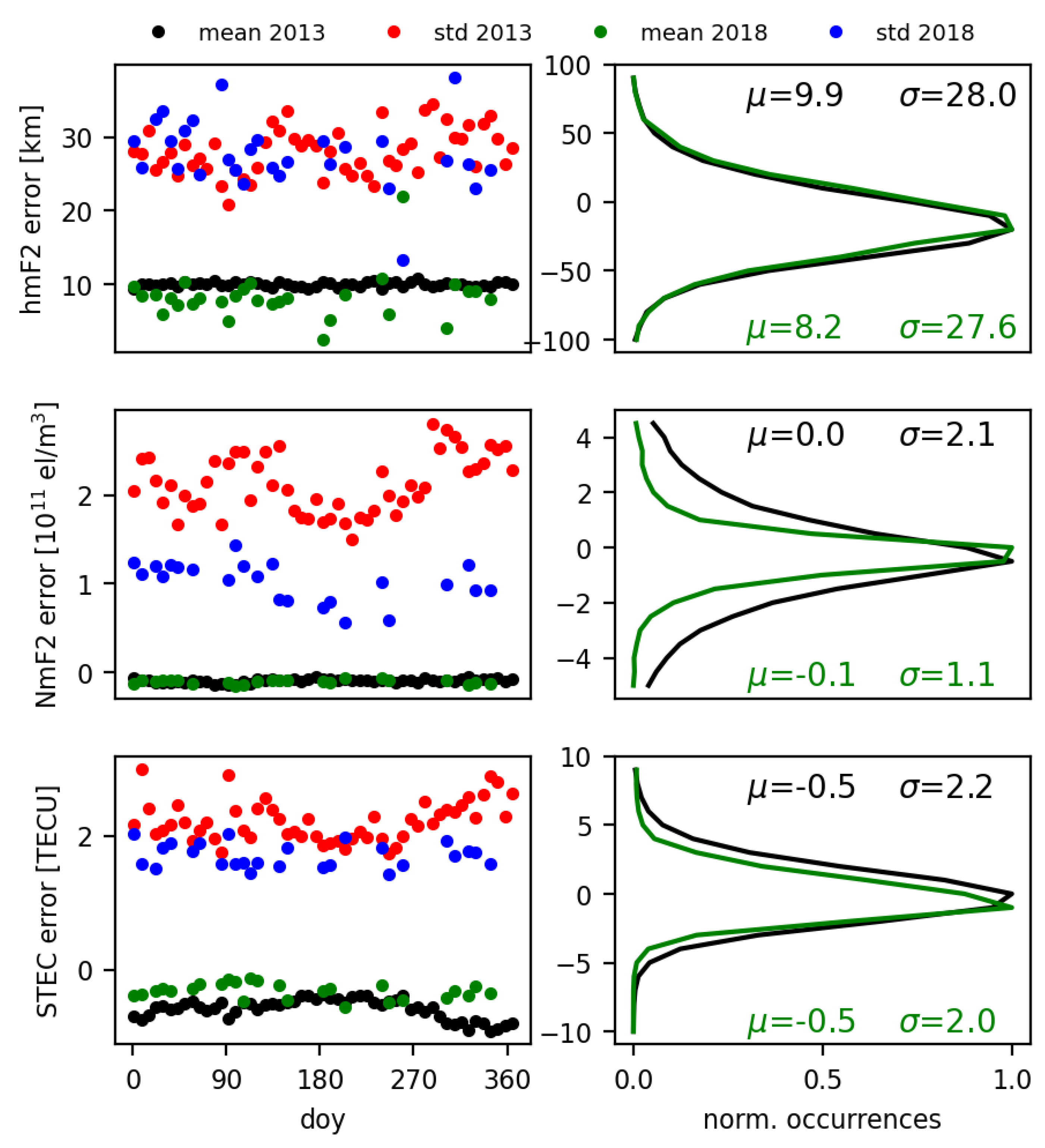
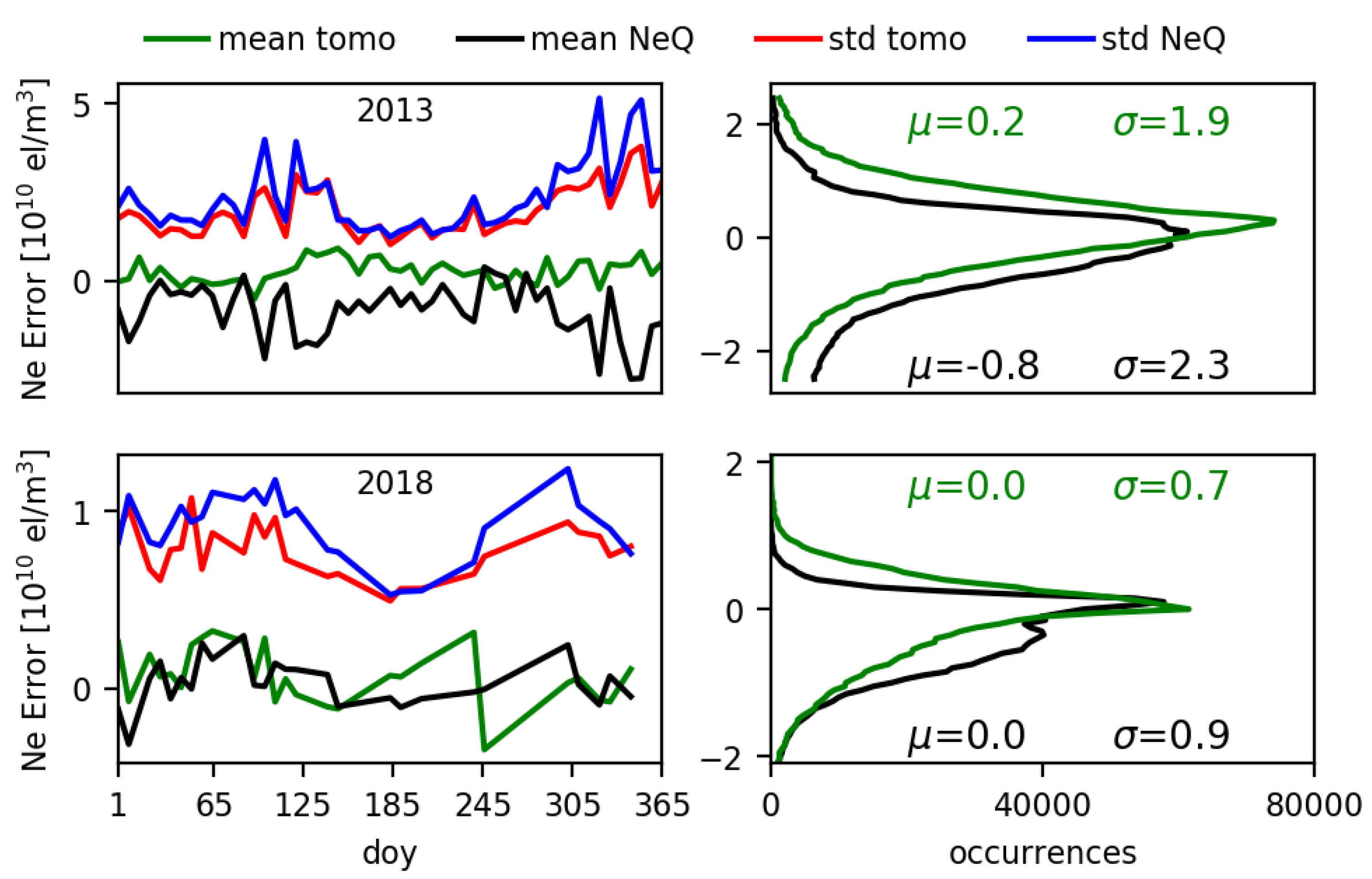
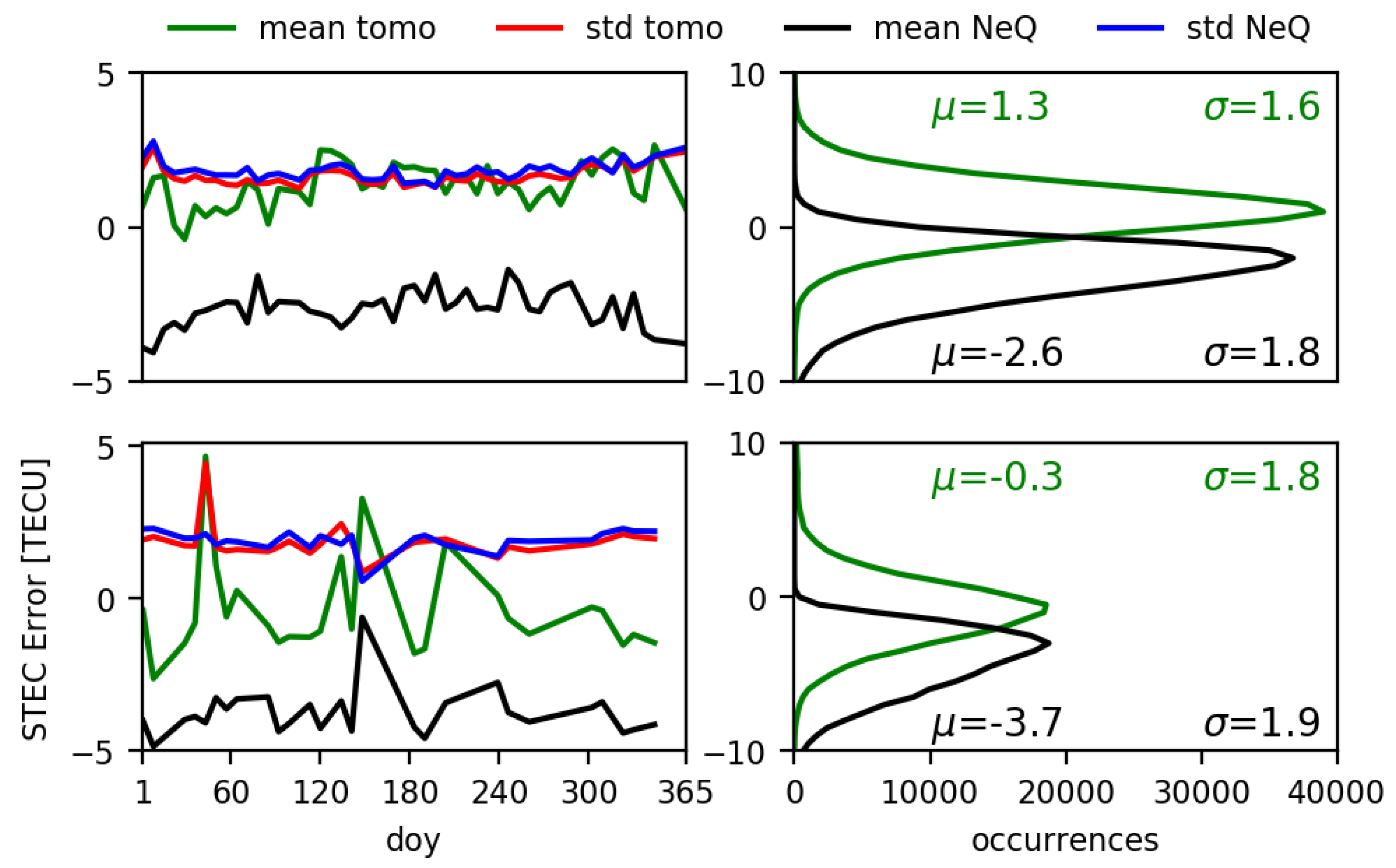
We first present general patterns of the developed model. Figure 1 shows daily maps of NmF2, hmF2 and VTEC obtained during the Northern solstice, equinox and Southern solstice of 2013 and 2018. All values were derived directly from the obtained 3D grid. Although the solution was obtained from discrete grids, we can observe very smooth results obtained for all parameters. Even during 2018, we can observe smoothed and typical distributions, which is a challenging task since there were very few COSMIC satellites operating in that year. Obvious patterns are observed that are related to the daily, seasonal and solar variabilities. Similar daily and seasonal variations are found by Prol et al. [6], where higher levels of ionization are observed near the maximum of the solar cycle during 2013 and lower levels of ionization are observed near the solar minimum of 2018.
In order to show vertical distributions of the reconstructed plasmasphere, Figure 2 presents meridional cross-sections of electron densities during nighttime and daytime for distinct years and seasons. The left side of each graph represents the nighttime (0 LT), and the right side of each graph represents the daytime (12 LT). Previous results [9] correspond to the one presented here, where we can clearly observe the natural variability of the electron density along the geomagnetic field lines. The plasmasphere extends up to a few Earth radii at the equator and diminishes toward the poles, with the intensity of ionization depending on the season and solar activity, being more intense in the summer of 2013. In addition to these typical distributions, significant low ionization at the Poles, especially during low solar activity and winter conditions, shows the absence of magnetic field lines at the Poles. These lower values occur in both conditions of 2013 and 2018, but this is more evident in 2018 due to the lower level of ionization.

4.2. Residuals

The quality control of the developed method was first performed to check how well the method adapts to the observation data, i.e., we first performed a self-consistency validation, where the residuals are analyzed. Figure 3 summarizes the tomographic residuals for hmF2, NmF2 and slant TEC (STEC). Left graphs show the temporal series of the mean and standard deviation errors. The hmF2 and NmF2 errors were computed using h m F 2 T O M O h m F 2 R O and N m F 2 T O M O N m F 2 R O , where TOMO stands for the tomographic results and RO for the direct measurements. The STEC error was computed using S T E C T O M O S T E C C O S M I C . The right panel of Figure 3 shows the histogram of errors considering all measurements of 2013 and 2018.
Figure 3 shows quite small hmF2 residuals with a mean error of about 10 km and standard deviation of about 30 km, which is compatible with the altitude resolution of 20 km. The mean and standard deviations are quite similar in 2013 and 2018. The results also present a quasi-Gaussian distribution in the histogram, which is mainly because the used harmonic function accommodates well to describe temporal and spatial distributions of hmF2. A small positive bias of 10 km has been obtained, which occurs due to the altitude resolution of 20 km. Indeed, for practical reasons, we compute the voxel position of a given altitude rounding up the voxel position to an integer value, creating a positive bias which is half of the altitude step size. Since this is a reasonable and minor error, we preferred to keep the bias instead of applying any post-process in the reconstruction just to extract hmF2.
Another result of the residual analysis is that the spatial and temporal features of NmF2 distributions are much harder to accommodate by the developed harmonic functions in comparison to hmF2. The NmF2 residual depends even more on the solar activity than the TEC error; where the standard deviation in 2018 is two times less than in 2013 for NmF2. Unlike the topside VTEC, NmF2 values should represent the two crests of the equatorial ionization anomaly; in addition, the F2-layer peak is more directly influenced by the solar photoionization than the total electron content of the topside ionosphere and plasmasphere. However, in any case, the mean and standard deviation are relatively small, providing a Gaussian distribution of the errors in the histogram. In the case of the STEC residuals, we see that measurements in the global 3D grid were enough to provide a low mean error of about 0.5 TECU with a dispersion of 2 TECU.

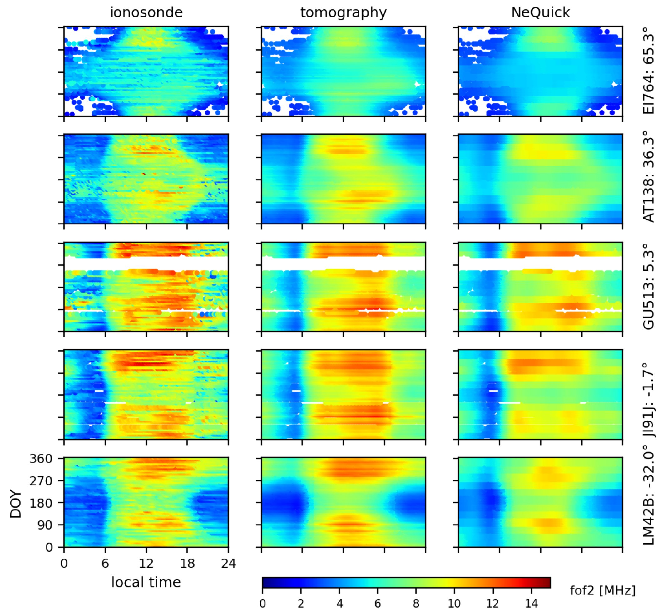
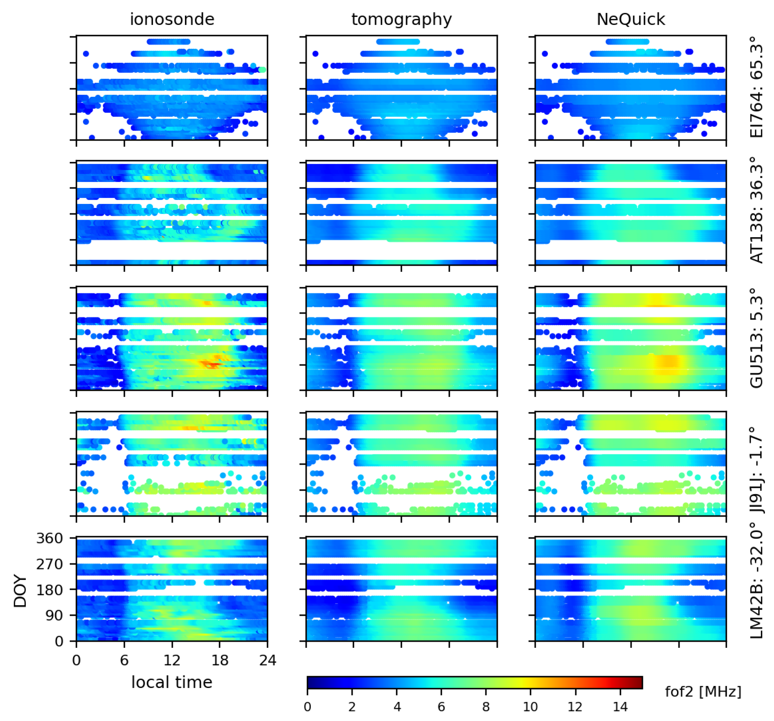
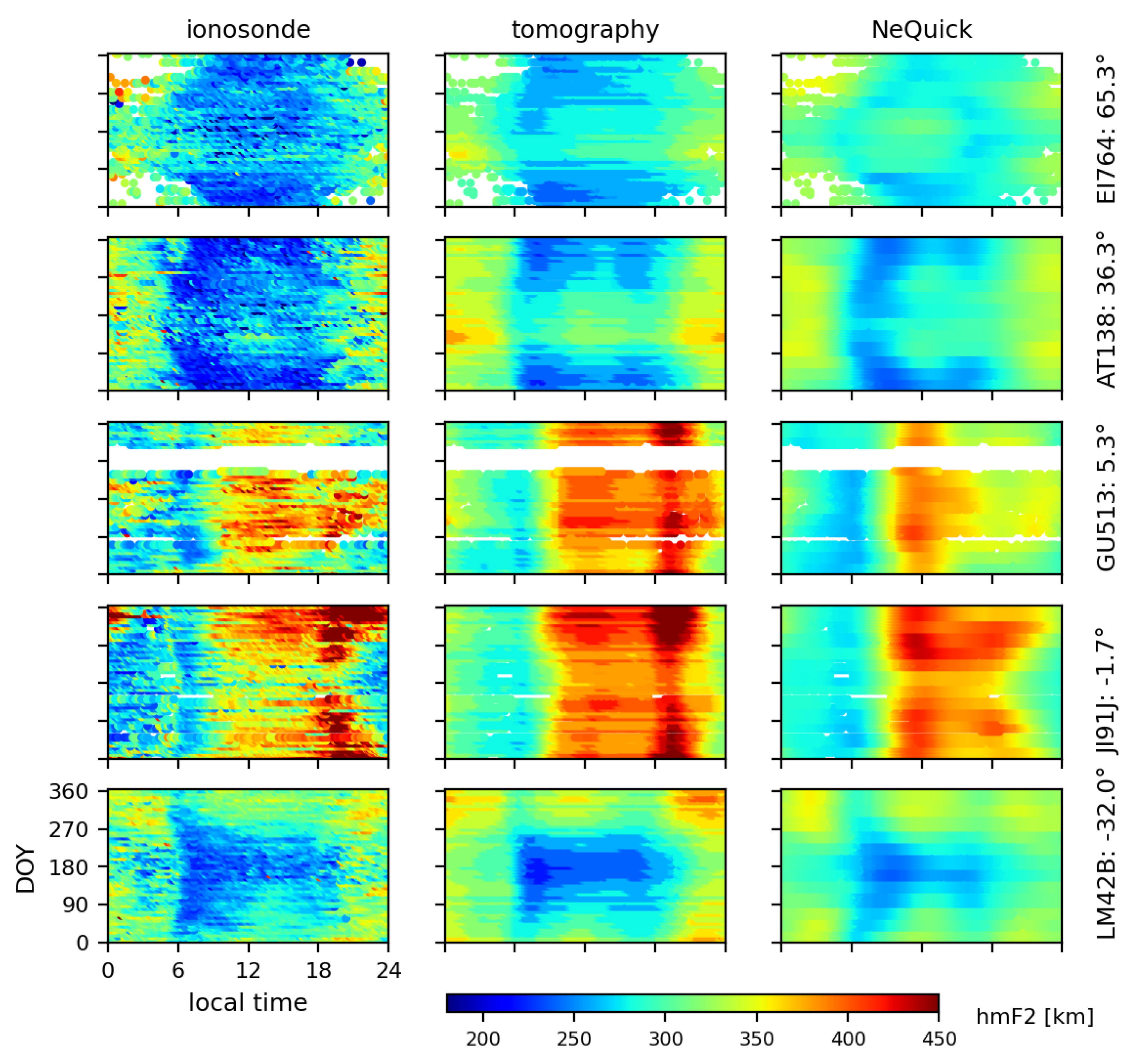
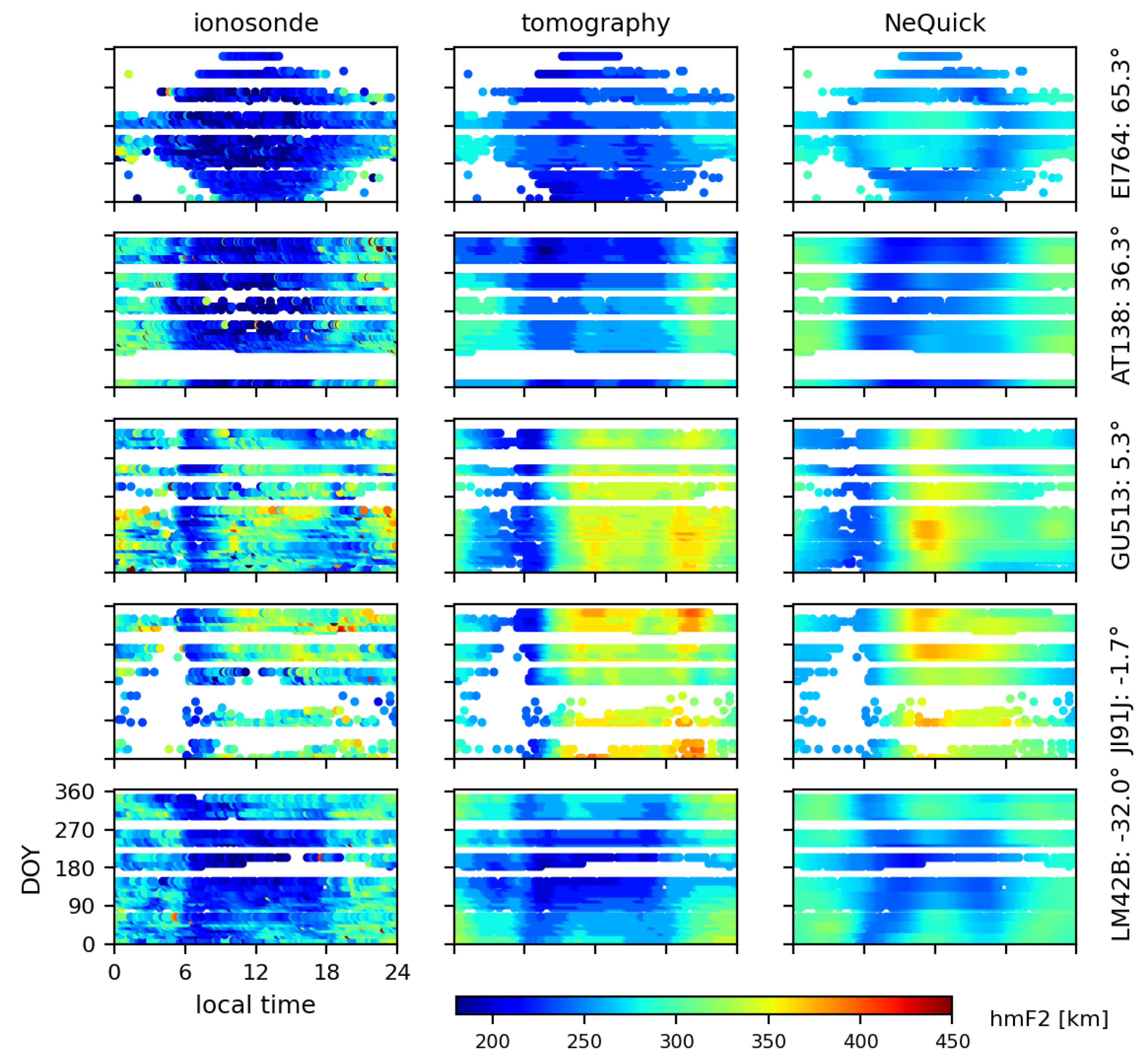
4.3. Assessment Using Ionosonde Data

The F2 layer peak electron density and its altitude are validated using GIRO ionosonde data as a reference. We have gathered all available GIRO data for the dates of interest, summing up a total of 52 and 63 stations for 2013 and 2018, respectively. In order to present the result in a comprehensive way, we have selected five representative stations for the main analyses. Figure 4 shows the estimated critical frequency (foF2) during 2013 of five ionosondes in distinct magnetic latitudes: EI764 located in Alaska (64.7° N, 212.9° E—mag. lat. 65.3° N), AT138 in Greece (38.0° N, 23.5° E—mag. lat. 36.3° N), GU513 in Guam (13.6° N, 144.8° E—mag. lat. 5.3° N), JI91J in Peru (−12.0° N, 283.2° E—mag. lat. −1.7° N), and LM42B in Australia (−21.8° N, 114.1° E—mag. lat. −32.0° N). For each specific location, the graph shows ionosonde, tomography and NeQuick values as functions of DOY and local time, so that we can observe the daily and seasonal distributions in distinct magnetic latitude regions. Figure 5 shows the same graph but for 2018. It is worth mentioning that the NeQuick uses CCIR (Comité Consultatif International des Radiocommunications) maps to describe hmF2 and NmF2 distribution; therefore, the observed accuracy of NeQuick can be understood as the accuracy of the CCIR maps.
As expected, the seasonal and daily distributions are well defined by the foF2 distributions, which are mostly controlled by the solar ionization. Higher foF2 values are observed at the equatorial region (GU513 and JI91J), reaching maximum values in the equinoxes around DOY 90 and 270 at the daytime of 2013. On the opposite, minimum values are observed in the winter solstices at middle and high latitudes of the nighttime of 2018. All of these patterns were observed by tomography and NeQuick. Actually, tomography and NeQuick were excellent at replicating the major distributions of the ionosondes, presenting a high level of agreement in the foF2 magnitude and variabilities. Indeed, there are just a few cases where significant errors can be visually observed, such as the under-estimation by NeQuick during the 2013 equinoxes at AT138 and LM42B and the under-estimation by tomography during the 2018 equinoxes at GU513 and JI91J.
The hmF2 patterns are shown in Figure 6 and Figure 7. Both methods have replicated the distributions. It was only the middle and high latitudes of 2013 where stations AT138, EI764 and LM42B presented reduced hmF2 values in the daytime that were not described by tomography and NeQuick. We see a general overestimation by both models and there is scope for improvements in cases of high solar activities. In 2018, the daily distributions at middle and high latitudes were better described by tomography. NeQuick presented significant visual discrepancies in 2018.
In case of the low-latitudes at the equatorial region, the daytime hmF2 is higher due to the ExB drift that uplifts the F-layer of the ionosphere. NeQuick and tomography have replicated such daily variability. Tomography was even capable of representing the subtle hmF2 increase around 18 LT, known to be related to the pre-reversal enhancement of the equatorial ionosphere due to the transition from daytime to nighttime [29]. Tomography results were more realistic of representing such pre-reversal enhancement, however with overestimated values for the station GU513 in 2013 and general over estimations for stations GU513 and JI91J in 2018.
Despite a few inconsistencies of tomography and NeQuick to describe spatial and temporal variabilities of foF2 and hmF2, high accuracy is obtained with both methods when looking at general statistics indicators. Figure 8 shows the histogram of foF2 errors in the top panels and the histogram of hmF2 errors in the bottom panels. This analysis was carried out considering 52 and 63 stations for 2013 and 2018, respectively. The graphs suggest an almost Gaussian distribution of the errors for tomography and NeQuick. Indeed, both models presented similar levels of accuracy with mean deviations of about 0.2 MHz and 10 km for foF2 and hmF2, respectively. The corresponding standard deviations are also similar for both methods, with around 1 MHz for foF2 and 40 km for hmF2. Therefore, no significant difference has been observed in the general accuracy of foF2 and hmF2 between the proposed method and NeQuick. The peak height of the proposed method is mainly controlled by the RO inversion, whereas the peak height of NeQuick is driven by the CCIR coefficients. Our investigation thus shows that the GNSS-based RO inversion can provide the peak of the ionosphere with a similar accuracy level as the method recommended by ITU (International Telecommunication Union).

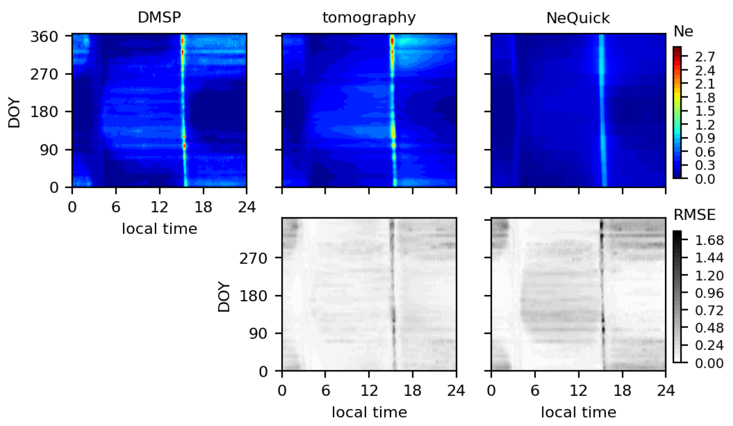
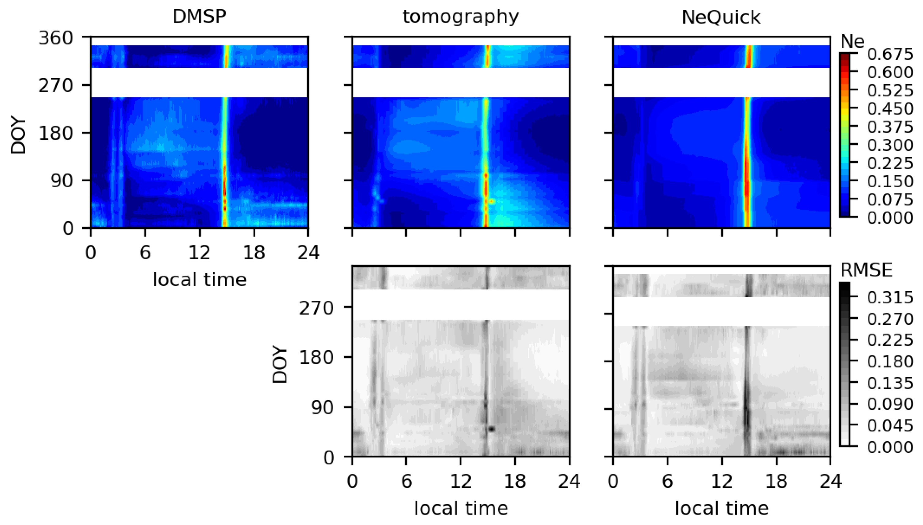
4.4. Assessment Using DMSP Data

The external quality assessment using DMSP is based on in situ electron density measurements from satellite number 15. It is worth mentioning that the DMSP satellite is flying around 800 km. The estimation of the proposed model in such a region is mainly controlled by the performance of the extrpolation of the Vary-Chap function to upper altitudes. This means that no direct measurements were used to describe the electron density in such altitudes. We are mainly relying on the ability of RO to describe four key parameters (hmF2, NmF2, Hs and dHs/dh) with good coverage in order to capture the vertical, horizontal and temporal features of the upper ionosphere.
Figure 9 shows the performance of the developed method during the entire year of 2013. The first graph on the left shows the daily averages of the DMSP electron density as a function of local time. The DMSP satellites have Sun-syncronous polar orbits with 98.9° inclination and 101.6 min period. The DMSP-15 position is located near the southern middle and high latitudes at 0 h LT. Then, the satellite flies in the direction of the nighttime equator, where a few in situ measurements are collected at a nighttime equator at around 03 h LT. After that, the satellite flies for a long time between 06–12 LT in the northern middle- and high-latitudes, passing through the North Pole around 08 LT. Due to the orbit geometry, just a few minutes are spent in the equatorial region, observing a small number of measurements in the low-latitudes. The nearly straight line of high ionization in the graphs is related to the accumulated measurements when the satellite is passing through the daytime equator at around 15 h LT. Measurements between 18–24 h LT again refer to the southern middle and high latitudes.
Overall, a very high level of agreement can be seen between the tomographic estimations and DMSP values. The developed model was able to capture all latitudinal, daily and seasonal variabilities seen by DMSP. We can see a good representation of the northern enhancement at around 06–12 h LT for DOYs 90–270, which refers to the time when the Sun was in the northern hemisphere. A symmetrical decrease of ionization is seen in the southern hemisphere between 18 and 24 h LT for the same DOYs. The DOYs 0–90 and 270–365 are related to the period when the Sun mainly ionizes the southern hemisphere. As expected, higher electron densities can be seen between 18–24 h LT and lower electron densities between 06–12 h LT. Compared to the NeQuick estimations, a higher level of agreement can also be noticed with our method. Indeed, NeQuick tends to underestimate the electron density ionization, mainly in the daytime equatorial region (e.g., see the straight line of high ionization).
Good agreements between tomography and DMSP can also be observed in 2018 (Figure 10), which reveals the proposed method as a capable tool to adapt to the solar cycle variabilities, even considering the reduced number of COSMIC satellites in 2018. However, it needs to be mentioned that the RMSE still presents some inconsistencies in the tomography, more evident in the daytime equatorial region. In 2018, two peaks in the nighttime equatorial region (around 03 h LT) are also noticeable. We attribute these two peaks related to the two crests formed by the Equatorial Ionization Anomaly (EIA), where neither NeQuick nor our model was capable of detecting the signatures at 800 km. Indeed, NeQuick shows an inverse behavior in comparison to 2013. The NeQuick results for 2018 show an overestimation at the daytime equator, where overestimations at the daytime equator are the main source of errors.
A complete overview of the DMSP evaluation during 2013 and 2018 is shown in Figure 11. As we can see, the developed approach was capable of showing the entire dataset with no significant biases, despite an expected higher standard deviation in the equinoxes of 2013. In comparison to NeQuick, the tomography has presented improvements. The root mean square error (RMSE) in 2013 of tomography was 2.01 × 10 10 el/m 3 and the RMSE of NeQuick was 2.48 × 10 10 el/ m 3 , which indicates an improvement of 19%. In 2018, the tomography RMSE was 0.79 × 10 10 el/ m 3 and the NeQuick RMSE was 0.91 × 10 10 el/ m 3 , which represents an improvement of 13%. Therefore, a general improvement around 15% was obtained with tomography.

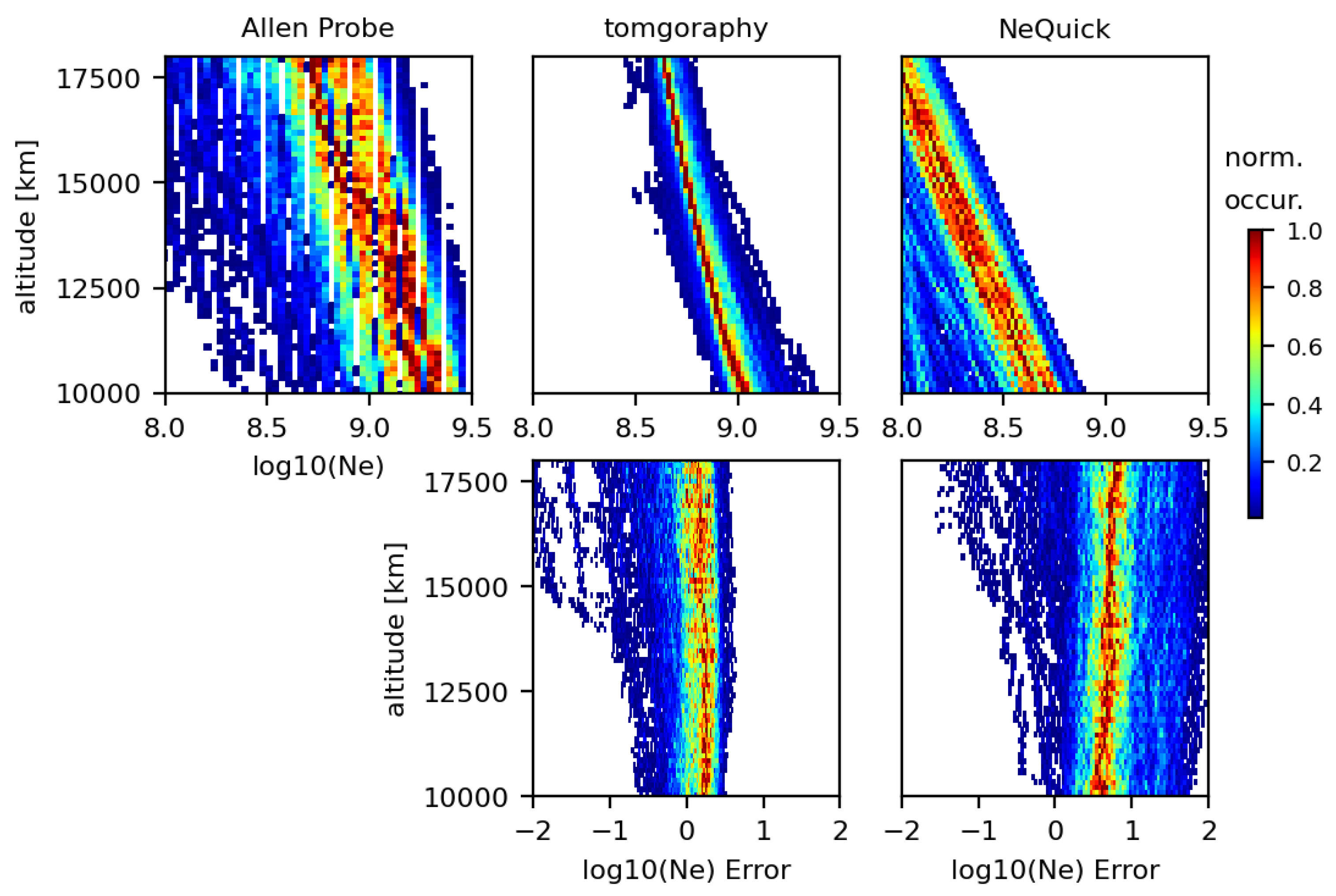
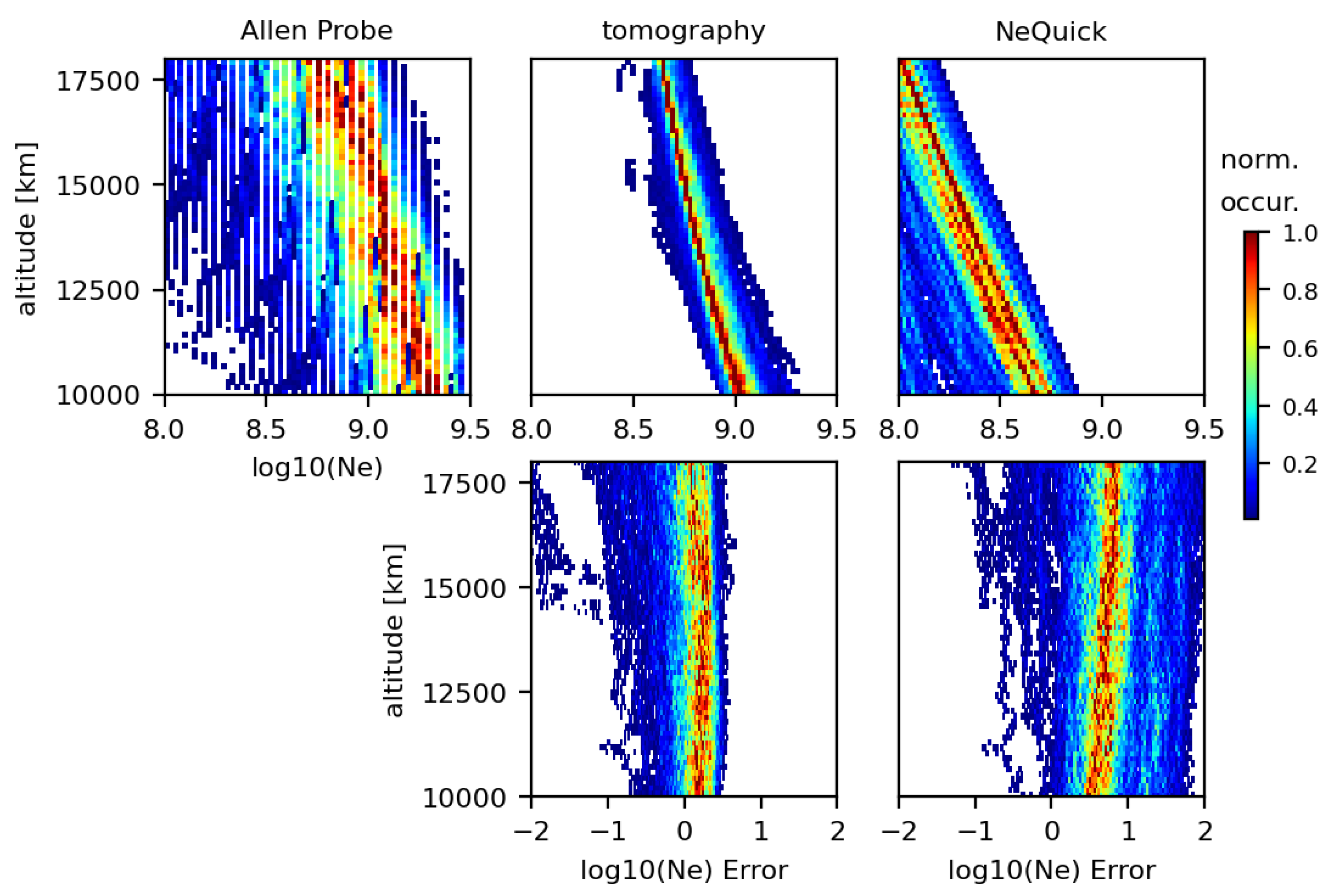
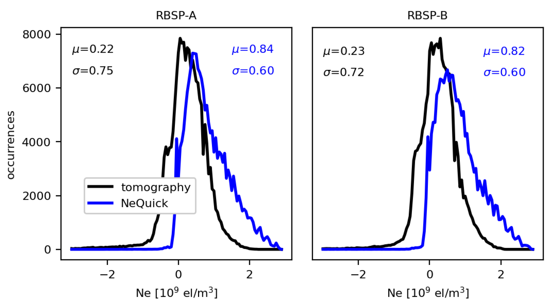
4.5. Assessment Using Van Allen Probes Data

To evaluate the top-most part of the plasmasphere, electron density values from the Van Allen Probes were taken as references. The Ne measurements are related to the satellite path with respect to its location in the plasmasphere. As the satellite flies upward or downward, individual profiles can be obtained. Figure 12 shows all individual Ne profiles superimposed as a function of the electron density and altitude. The distributions are shown in terms of the normalized number of occurrences in the log scale by taking the number of occurrences of a specific pixel in the 2D-histogram and dividing it by the maximum value of occurrences in the specific height. The bottom panels show the electron density errors of tomography and NeQuick when compared to the values obtained from RBSP-A instrument. Figure 13 shows the same, but for the RBSP-B instrument. Only 2013 was analyzed here since Van Allen Probes data from the NURD algorithm are still not available for 2018.
Despite the simple approach used to extrapolate the RO profiles to the plasmasphere, a high level of agreement can be seen between the tomography and Van Allen Probes distributions for altitudes very far from those where the RO observations were taken. This indicates that the linear interpolation in the log scale between 800 km and the plasmapause, with a minimum electron density as 4 × 10 8 el/m 3 at the end point of the plasmasphere, was enough to capture magnitudes and the main patterns of the plasmasphere. The tomographic profiles are closer to the Van Allen Probes data than the NeQuick profiles. However, there is still a bias in the tomography profiles, which is minor and around 2 × 10 8 el/m 3 (Figure 14), whereas the NeQuick solution presents an overall bias of 8 × 10 8 el/m 3 . In total, the tomography RMSE using the RBSP-A instrument was 8.25 × 10 8 el/m3 and the NeQuick RMSE was 11.03 × 10 8 el/m 3 . The total RMSE using the RBSP-B instrument was 8.05 × 10 8 el/m 3 for tomography and 10.98 × 10 8 el/m 3 for NeQuick. The developed method thus resulted in an improvement of 26%.

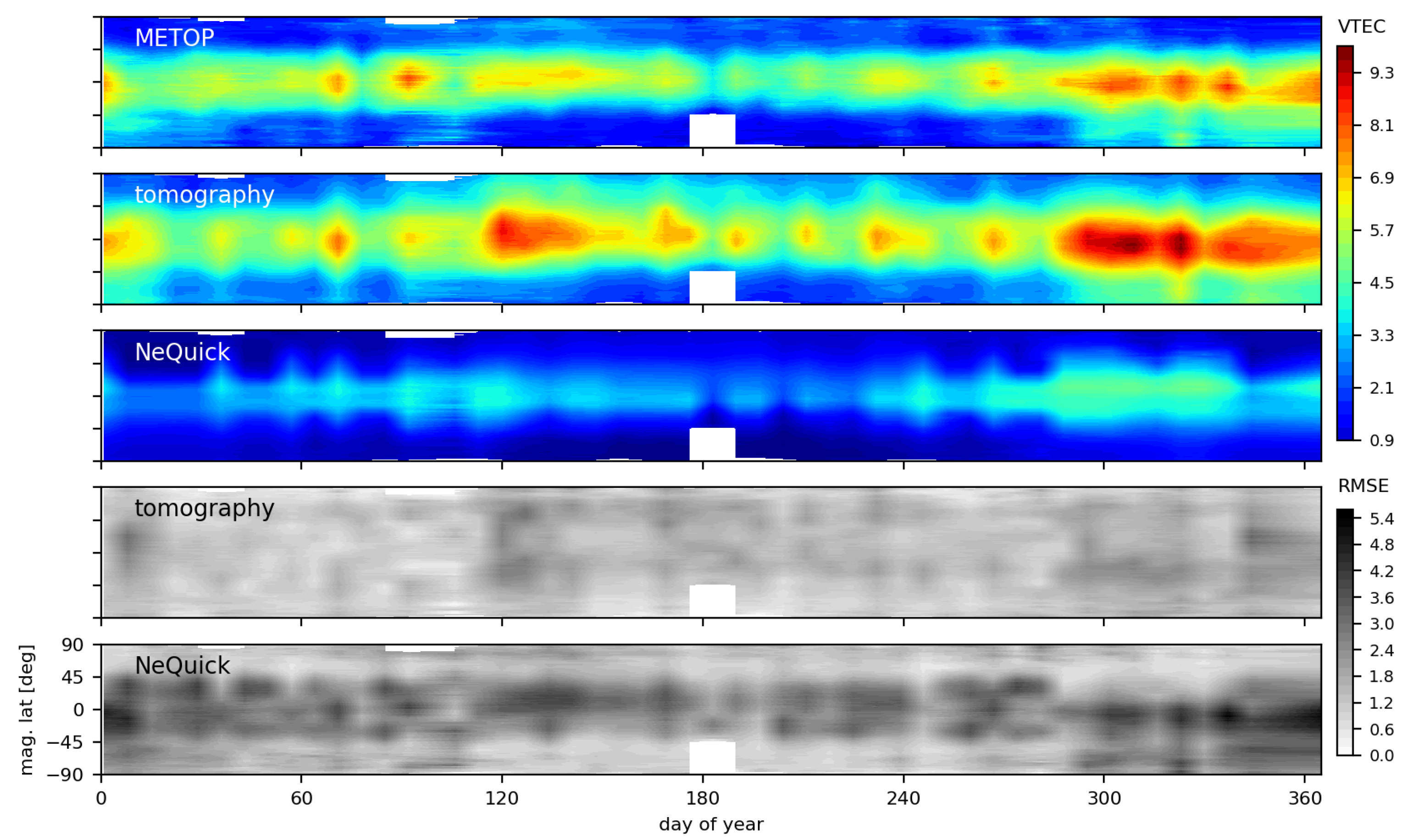
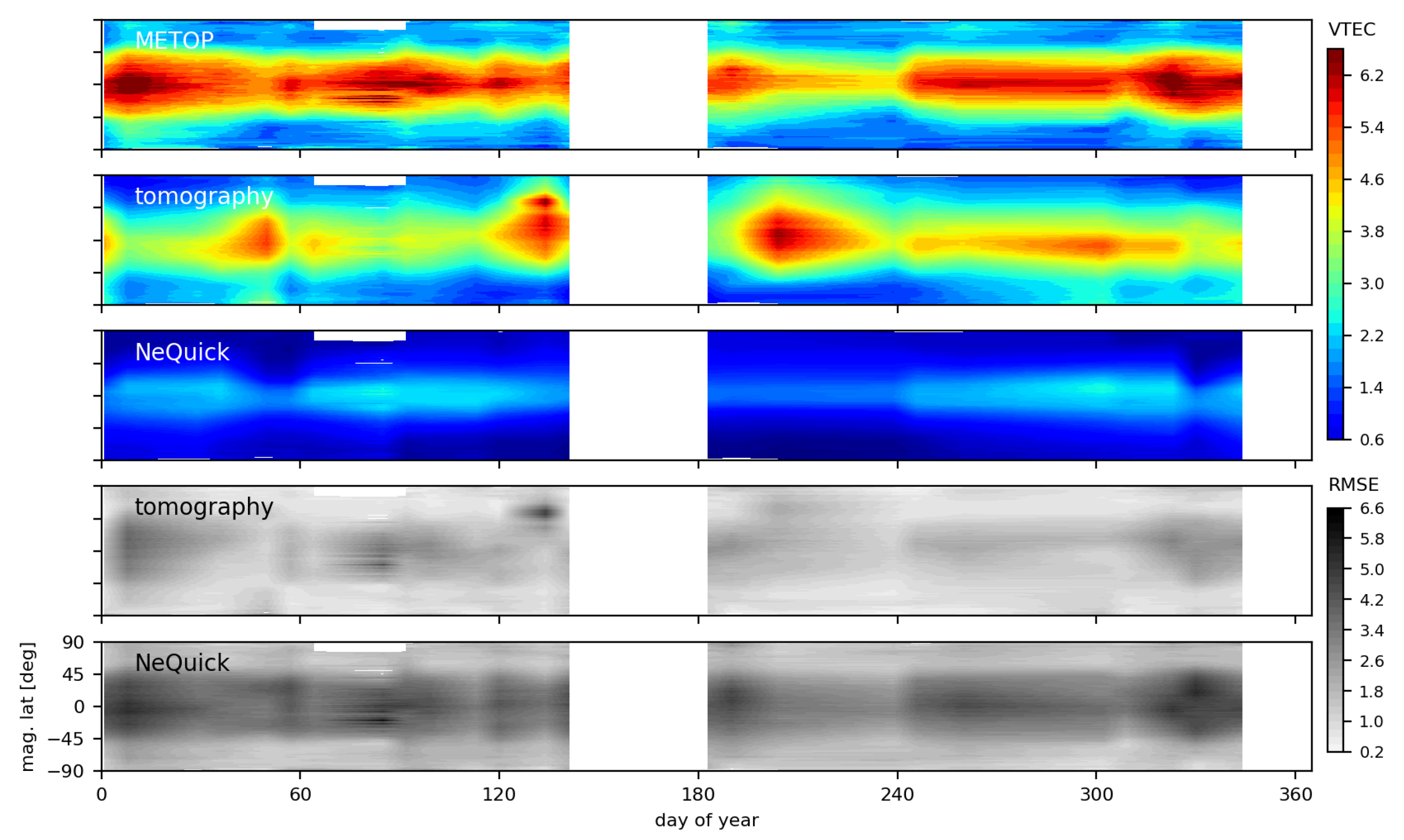
4.6. Assessment Using METOP Data

The assessment using METOP measurements was carried out to include independent reference STEC values in the model performance evaluation. After converting STEC to VTEC and taking the daily average along the magnetic latitude, we can observe the general TEC distributions of METOP data during the entire two years. Figure 15 and Figure 16 (top panel) show the VTEC distribution obtained with METOP data during 2013 and 2018, respectively. The two bottom panels show model performance in terms of RMSE. All distributions were built considering the rising phase of the METOP satellite in order to take data collected at a similar LT into account. Indeed, at a giving location, the satellite will rise from the horizon, pass overhead and then set in the opposite horizon. Since the satellite orbit is almost polar, we have defined the rising phase related to the South to North direction with an increasing LT, while the setting phase is related to the North to South direction. As shown by Prol et al. [28], the METOP orbit configuration can provide distinct VTEC distributions during the rising and setting phases; however, in the present study, similar conclusions and accuracy of Figure 15 and Figure 16 are obtained when considering VTEC values during the setting phase of the METOP satellite.
Natural VTEC variabilities can be observed in the METOP distributions of 2013, where there are obvious enhancements in the Southern hemisphere in the corresponding solstice (see DOYs 1 to 30 and after 300 in Figure 15) and a considerable VTEC decrease in the winter period. The same happens for the Northern hemisphere; however, tomography has presented overestimated results in the Northern summer of 2013. There are probably significant differences between the METOP and COSMIC orbits in this period of the year. Since both constellation orbits are passing through distinct regions with a very repetitive daily pattern, a few systematic discrepancies are expected. We therefore highlight that the VTEC distributions of the topside depend significantly on the dataset used to perform the tomography, but it is important to note that our developed model can be easily adapted to use METOP measurements as input data. Additionally, when looking at the NeQuick estimations, all cases show a general underestimation. As presented in previous works [30], NeQuick systematically presents lower TEC values in comparison to satellite-based POD TEC measurements, but now we confirm a similar trend of underestimation in the case of METOP measurements for 2013 and 2018.
A statistical overview of the models performance using METOP POD TEC data during 2013 and 2018 is shown in Figure 17. The errors were computed using the following expressions: S T E C N e Q S T E C M E T O P and S T E C T O M O S T E C M E T O P . As expected from the previous analysis, we can observe a tomographic overestimation in the year of high solar activity (2013), with a general bias of 1.6 TECU. On the other hand, no systematic error has been found for tomography in 2018. In the case of NeQuick, we have observed relevant underestimations in all days and years, but a similar standard deviation when compared to tomography. Similar TEC biases around −4 to −2 TECU of the default NeQuick model are observed by [31] when comparing with TEC data of COSMIC and SWARM satellites. In total, the tomography RMSE in 2013 was 2.3 TECU and the NeQuick RMSE was 3.1 TECU, which indicates an improvement of 26% in epochs of high solar activity. The RMSE in 2018 was 1.8 TECU for tomography and 4.2 TECU for NeQuick, which shows a relevant improvement of 55% for low solar activities. The proposed NeQuick improvement by [31] is an appealing option to obtain better NeQuick biases and further analysis may improve the NeQuick results. From their results, a bias around −3 to −2 TECU is expected in the VTEC estimation based on the new formulation; however, there is still room for improvement to obtain an almost zero bias in NeQuick.

5. Conclusions

A model that depends only on satellite-based GNSS measurements has been developed to describe the upper ionosphere and plasmasphere from hmF2 up to the plasmapause. Describing this region of the ionosphere and plasmasphere with climatological models, such as NeQuick and IRI, has presented continuous challenges [4]. At the peak of the ionosphere, the proposed method based on RO has provided a similar level of accuracy as NeQuick, revealing that GNSS-based RO inversion can present the peak of the ionosphere with a similar level of accuracy as the method recommended by ITU. Nevertheless, significant improvements were obtained in comparison to NeQuick when validated against external VTEC data from METOP and Ne data from DMSP and Van Allen Probes. The proposed method therefore provides a good specification of the variability of the upper ionosphere and plasmasphere.
The high agreement with DMSP and Van Allen Probes electron density values was mainly obtained due to the Vary-Chap function and RO observations. This yields to the conclusion that the linear scale height together with the proposed extrapolation scheme represent a powerful tool to describe the plasmasphere and upper ionosphere. Past validations, such as Olivares-Pulido et al. [23] and Prol et al. [6], have also confirmed the high accuracy of RO and Vary-Chap on the topside, but now we have proved their capabilities using DMSP data as a reference.
Since only GNSS data are required, the developed approach does not depend on traditional empirical models. As shown in the results, our approach is applicable even when a unique COSMIC satellite is operating. The only one requirement is that historical data of up to one-year with global coverage have been used here. Global coverage is still a viable resource for the coming years due to the continuous densification of GNSS receivers onboard LEO satellites. However, future investigations are still necessary mainly to check model capabilities to represent the topside features during storm conditions. Additionally, further data fusion with bottomside measurements is still necessary for a complete specification of the ionosphere and recent improvements in NeQuick [31,32] should also be considered in future analysis.

Author Contributions

Conceptualization, F.S.P. and M.M.H.; methodology, F.S.P. and M.M.H.; software, F.S.P.; validation, F.S.P.; formal analysis, F.S.P. and M.M.H.; investigation, F.S.P. and M.M.H.; resources, M.M.H.; writing—original draft preparation, F.S.P.; writing—review and editing, M.M.H.; visualization, F.S.P.; supervision, M.M.H.; project administration, M.M.H.; funding acquisition, M.M.H. All authors have read and agreed to the published version of the manuscript.

Funding

This work has been funded by the Deutsche Forschungsgemeinschaft (DFG) under Grant No. HO 6136/1-1 and by the ‘Helmholtz Pilot Projects Information & Data Science II’ (grant support from the Initiative and Networking Fund of the Hermann von Helmholtz-Association Deutscher Forschungszentren e.V. (ZT-I-0022)) with the project named ‘MAchine learning based Plasma density model’ (MAP).

Data Availability Statement

The used GIRO datasets were downloaded from the portal http://giro.uml.edu/didbase/scaled.php (accessed on 10 March 2021). The used DMSP electron density data are processed by the Center for Space Sciences at the University of Texas (Dallas) and obtained through the Madrigal portal http://cedar.openmadrigal.org/ (accessed on 10 March 2021). The NURD dataset is available at ftp://rbm.epss.ucla.edu/ftpdisk1/NURD (accessed on 10 March 2021). The used METOP-A data are processed by UCAR and downloaded through the CDAAC archive at https://cdaac-www.cosmic.ucar.edu/ (accessed on 10 March 2021). The International Geomagnetic Reference Field (IGRF) is available at https://www.ngdc.noaa.gov/IAGA/vmod/igrf.html (accessed on 10 March 2021).

Acknowledgments

The authors would like to thank the University Corporation for Atmospheric Research, Boulder, CO, USA, and National Space Organization, Hsinchu, Taiwan, for providing FORMSAT-3/COSMIC and METOP data. They would also like to thank the developers of the Defense Meteorological Satellite Program (DMSP). The NeQuick model was developed at the T/ICT4D Laboratory of the Abdus Salam International Centre for Theoretical Physics. The authors would like to thank all members responsible at the GIRO project. We also thank the developers of NURD and Van Allen Probes.

Conflicts of Interest

The authors declare no conflict of interest.

References

  1. Nava, B.; Coisson, P.; Radicella, S.M. A new version of the NeQuick ionosphere electron density model. J. Atmos. Sol. Terr. Phys. 2008, 70, 1856–1862. [Google Scholar] [CrossRef]
  2. Gulyaeva, T.L.; Titheridge, J.E. Advanced specification of electron density and temperature in the IRI ionosphere—Plasmasphere model. Adv. Space Res. 2006, 38, 2587–2595. [Google Scholar] [CrossRef]
  3. Tariku, Y.A. Validation of the IRI 2016, IRI-Plas 2017 and NeQuick 2 models over the West Pacific regions using the SSN and F10.7 solar indices as proxy. J. Atmos. Sol. Terr. Phys. 2019, 195, 105055. [Google Scholar] [CrossRef]
  4. Cherniak, I.; Zakharenkova, I. NeQuick and IRI-Plas model performance on topside electron content representation: Spaceborne GPS measurements. Radio Sci. 2016, 51, 752–766. [Google Scholar] [CrossRef] [Green Version]
  5. Gulyaeva, T.L. Storm time behavior of topside scale height inferred from the ionosphere—Plasmasphere model driven by the F2 layer peak and GPS-TEC observations. Adv. Space Res. 2011, 47, 913–920. [Google Scholar] [CrossRef]
  6. Prol, F.S.; Hernández-Pajares, M.; Camargo, P.O.; Muella, M.T.A.H. Spatial and temporal features of the topside ionospheric electron density by a new model based on GPS radio occultation data. J. Geophys. Res. Space Phys. 2018, 123, 2104–2115. [Google Scholar] [CrossRef]
  7. Li, Q.; Liu, L.; Jiang, J.; Li, W.; Huang, H.; Yu, Y.; Li, J.; Zhang, R.; Le, H.; Chen, Y. α-Chapman scale height: Longitudinal variation and global modeling. J. Geophys. Res. Space Phys. 2019, 124, 2083–2098. [Google Scholar] [CrossRef]
  8. Wu, M.J.; Guo, P.; Chen, Y.L.; Fu, N.F.; Hu, X.G.; Hong, Z.J. New Vary-Chap scale height profile retrieved from COSMIC radio occultation data. J. Geophys. Res. Space Phys. 2020, 125, e2019JA027637. [Google Scholar] [CrossRef]
  9. Heise, S.; Jakowski, N.; Wehrenpfennig, A.; Reigber, C.; Lühr, H. Sounding of the topside ionosphere/plasmasphere based on GPS measurements from CHAMP: Initial results. Geophys. Res. Lett. 2002, 29, 1699. [Google Scholar] [CrossRef] [Green Version]
  10. Spencer, P.S.J.; Mitchell, C.N. Imaging of 3D plasmaspheric electron density using GPS to LEO satellite differential phase observations. Radio Sci. 2011, 46, RS0D04. [Google Scholar] [CrossRef] [Green Version]
  11. Wu, M.J.; Guo, P.; Xu, T.L.; Fu, N.F.; Xu, X.S.; Jin, H.L.; Hu, X.G. Data assimilation of plasmasphere and upper ionosphere using COSMIC/GPS slant TEC measurements. Radio Sci. 2015, 50, 1131–1140. [Google Scholar] [CrossRef] [Green Version]
  12. Gallagher, D.L.; Craven, P.D.; Comfort, H. Global core plasma model. J. Geophys. Res. 2000, 105, 18819–18833. [Google Scholar] [CrossRef]
  13. Schreiner, W.S.; Weiss, J.P.; Anthes, R.A.; Braun, J.; Chu, V.; Fong, J.; Hunt, D.; Kuo, Y.-H.; Meehan, T.; Serafino, W.; et al. COSMIC-2 radio occultation constellation: First results. Geophys. Res. Lett. 2020, 47, e2019GL086841. [Google Scholar] [CrossRef]
  14. Forsythe, V.V.; Duly, T.; Hampton, D.; Nguyen, V. Validation of ionospheric electron density measurements derived from Spire CubeSat constellation. Radio Sci. 2020, 55, e2019RS006953. [Google Scholar] [CrossRef]
  15. Yue, X.; Schreiner, W.S.; Hunt, D.C.; Rocken, C.; Kuo, Y.-H. Quantitative evaluation of the low Earth orbit satellite based slant total electron content determination. Space Weather 2011, 9, S09001. [Google Scholar] [CrossRef] [Green Version]
  16. Reinisch, B.R.; Galkin, I.A. Global ionospheric radio observatory (GIRO). Earth Planets Space 2011, 63, 377–381. [Google Scholar] [CrossRef] [Green Version]
  17. Garner, T.W.; Taylor, B.T.; Gaussiran, T.L., II; Coley, W.R.; Hairston, M.R.; Rich, F.J. Statistical behavior of the topside electron density as determined from DMSP observations: A probabilistic climatology. J. Geophys. Res. 2010, 115, A07306. [Google Scholar] [CrossRef] [Green Version]
  18. Zhelavskaya, I.S.; Spasojevic, M.; Shprits, Y.Y.; Kurth, W.S. Automated determination of electron density from electric field measurements on the Van Allen Probes spacecraft. J. Geophys. Res. Space Phys. 2016, 121, 4611–4625. [Google Scholar] [CrossRef] [Green Version]
  19. Prol, F.S.; Themens, D.R.; Hernández-Pajares, M.; Camargo, P.O.; Muella, M.T.A.H. Linear Vary-Chap Topside Electron Density Model with Topside Sounder and Radio-Occultation Data. Surv. Geophys. 2019, 40, 277–293. [Google Scholar] [CrossRef]
  20. Foelsche, U.; Kirchengast, G. A simple “geometric” mapping function for the hydrostatic delay at radio frequencies and assessment of its performance. Geophys. Res. Lett. 2002, 29, 1473. [Google Scholar] [CrossRef] [Green Version]
  21. Zhong, J.; Lei, J.; Dou, X.; Yue, X. Assessment of vertical TEC mapping functions for space-based GNSS observations. GPS Solut. 2016, 20, 353–362. [Google Scholar] [CrossRef]
  22. Ssessanga, N.; Kim, Y.H.; Kim, E. Vertical structure of medium-scale traveling ionospheric disturbances. Geophys. Res. Lett. 2015, 42, 9156–9165. [Google Scholar] [CrossRef]
  23. Olivares-Pulido, G.; Hernández-Pajares, M.; Aragón-Angel, A.; Garcia-Rigo, A. A linear scale height Chapman model supported by GNSS occultation measurements. J. Geophys. Res. Space Phys. 2008, 121, 7932–7940. [Google Scholar] [CrossRef] [Green Version]
  24. Zhelavskaya, I.S.; Shprits, Y.; Spasojevic, M. Empirical Modeling of the Plasmasphere Dynamics Using Neural Networks. J. Geophys. Res. 2017, 122, 11227–11244. [Google Scholar] [CrossRef] [Green Version]
  25. Austen, J.R.; Franke, S.J.; Liu, C.H. Ionospheric imaging using computerized tomography. Radio Sci. 1988, 23, 299–307. [Google Scholar] [CrossRef]
  26. Wei, W.; Biwen, T.; Jiexian, W. Application of a simultaneous iterations reconstruction technique for a 3D water vapor tomography system. Geod. Geodyn. 2013, 4, 41–45. [Google Scholar] [CrossRef] [Green Version]
  27. Pryse, S.E.; Kersley, L. A preliminary experimental test of ionospheric tomography. J. Atmos. Sol. Terr. Phys. 1992, 54, 1007–1012. [Google Scholar] [CrossRef]
  28. Prol, F.S.; Hoque, M.M.; Ferreira, A.A. Plasmasphere and topside ionosphere reconstruction using METOP satellite data during geomagnetic storms. J. Space Weather Space Clim. 2021, 11, 5. [Google Scholar] [CrossRef]
  29. Prol, F.S.; Camargo, P.O.; Hernández-Pajares, M.; Muella, M.T.A.H. A New Method for Ionospheric Tomography and its Assessment by Ionosonde Electron Density, GPS TEC, and Single-Frequency PPP. IEEE Trans. Geosci. Remote Sens. 2019, 57, 2571–2582. [Google Scholar] [CrossRef]
  30. Kashcheyev, A.; Nava, B. Validation of NeQuick 2 model topside ionosphere and plasmasphere electron content using COSMIC POD TEC. J. Geophys. Res. Space Phys. 2019, 124, 9525–9536. [Google Scholar] [CrossRef]
  31. Pezzopane, M.; Pignalberi, A. The ESA Swarm mission to help ionospheric modeling: A new NeQuick topside formulation for mid-latitude regions. Sci. Rep. 2019, 9, 12253. [Google Scholar] [CrossRef] [PubMed] [Green Version]
  32. Pignalberi, A.; Pezzopane, M.; Nava, B.; Coïson, P. On the link between the topside ionospheric effective scale height and the plasma ambipolar diffusion, theory and preliminary results. Sci. Rep. 2020, 10, 17541. [Google Scholar] [CrossRef] [PubMed]
Figure 1. General patterns of the estimated values of NmF2 (10 12 el/m 3 ), hmF2 (km) and topside VTEC (10 16 el/m 2 ). The days of 2013 are related to days of year (DOY) 172, 264 and 356 for the Northern solstice, equinox and Southern solstice, respectively. DOYs of 2018 are related to 180, 264 and 359 for the Northern solstice, equinox and Southern solstice, respectively. These are the closest DOYs to the seasons of interest with actual COSMIC observations.
Remotesensing 13 01559 g001
Figure 2. Meridional cross-sections during solstices and equinoxes of 2013 (top panels) and 2018 (bottom panels). The unit of the color bar is el/m 3 .
Remotesensing 13 01559 g002
Figure 3. Overview of the residuals of the developed method in comparison to RO peak electron density and satellite-based TEC. The left panel shows the temporal series of the standard deviations and daily averages of the errors computed for 2013 and 2018. The right panel shows the histogram of normalized occurrences of the errors, with the corresponding mean ( μ ) and standard deviation ( σ ) of the differences.
Remotesensing 13 01559 g003
Figure 4. Critical frequency estimated in five ionosonde locations using the GIRO dataset (left), tomography (middle) and NeQuick (right) in terms of local time and the days of the year 2013. White spaces represent lack of data.
Remotesensing 13 01559 g004
Figure 5. Critical frequency estimated in five ionosonde locations using GIRO dataset (left), tomography (middle) and NeQuick (right) in terms of local time and day of year of 2018. White spaces represent lack of data.
Remotesensing 13 01559 g005
Figure 6. Peak height estimated in five ionosonde locations using GIRO dataset (left), tomography (middle) and NeQuick (right) in terms of local time and day of year of 2013. White spaces represent lack of data.
Remotesensing 13 01559 g006
Figure 7. Peak height estimated in five ionosonde locations using GIRO dataset (left), tomography (middle) and NeQuick (right) in terms of local time and day of year of 2018. White spaces represent lack of data.
Remotesensing 13 01559 g007
Figure 8. Histograms of foF2 and hmF2 errors from tomography and NeQuick when compared to ionosonde data for 2013 (left panels) and 2018 (right panels). The graph also shows model performance in terms of the overall mean ( μ ) and standard deviation ( σ ) of the differences.
Remotesensing 13 01559 g008
Figure 9. Electron density and RMSE distributions during 2013 obtained with DMSP number 15, NeQuick and tomography. The electron density Ne (el/m 3 ) was estimated based on a daily average in terms of local time.
Remotesensing 13 01559 g009
Figure 10. Electron density and RMSE distributions during 2018 obtained with DMSP number 15, NeQuick and tomography. The electron density Ne (el/m 3 ) was estimated based on a daily average in terms of local time. White spaces are referred to the lack of DMSP or COSMIC data.
Remotesensing 13 01559 g010
Figure 11. Electron density errors of the tomography and NeQuick with respect to the DMSP 15 satellite data. The left panel shows the temporal series of the standard deviations and daily averages of the errors computed for 2013 (top) and 2018 (bottom). The right panel shows the histogram of the errors together with the total error mean ( μ ) and standard deviation ( σ ) of the differences.
Remotesensing 13 01559 g011
Figure 12. 2D histogram of profiles from the Van Allen Probes RBSP-A instrument (top left), tomography (top middle) and NeQuick (top right) as a function of the altitude and logarithm of electron density with base 10. The bottom panels show the corresponding errors of the profiles. The color of the points represents the normalized occurrence.
Remotesensing 13 01559 g012
Figure 13. Same as Figure 12, but for the RBSP-B instrument.
Remotesensing 13 01559 g013
Figure 14. Histogram of the electron density error for tomography (black line) and NeQuick (blue line) when compared to Van Allen Probes estimations for 2013. The graph also shows the total mean ( μ ) error and standard deviation ( σ ) of the errors.
Remotesensing 13 01559 g014
Figure 15. VTEC and RMSE distributions during 2013 estimated with METOP, NeQuick and tomography. VTEC values were taken as a daily average in terms of magnetic latitude. White spaces refer to the lack of METOP or COSMIC data. Units are given in 10 16 el/m 2 .
Remotesensing 13 01559 g015
Figure 16. VTEC and RMSE distributions during 2018 estimated with METOP, NeQuick and tomography. VTEC values were taken as a daily average in terms of magnetic latitude. White spaces refer to the lack of METOP or COSMIC data. Units are given in 10 16 el/m 2 .
Remotesensing 13 01559 g016
Figure 17. Electron density errors of the tomography and NeQuick with respect to the METOP-A satellite data. The left panel shows the temporal series of the standard deviations and daily averages of the errors computed for 2013 (top) and 2018 (bottom). The right panel shows the histogram of the errors together with the total error mean ( μ ) and standard deviation ( σ ) of the differences.
Remotesensing 13 01559 g017
Publisher’s Note: MDPI stays neutral with regard to jurisdictional claims in published maps and institutional affiliations.

